| Issue |
A&A
Volume 687, July 2024
|
|
|---|---|---|
| Article Number | A290 | |
| Number of page(s) | 11 | |
| Section | Stellar structure and evolution | |
| DOI | https://doi.org/10.1051/0004-6361/202449782 | |
| Published online | 22 July 2024 | |
Evolution of rotating massive stars adopting a newer, self-consistent wind prescription at Small Magellanic Cloud metallicity
1
Nicolaus Copernicus Astronomical Center, Polish Academy of Sciences, Bartycka 18, 00-716 Warsaw, Poland
e-mail: This email address is being protected from spambots. You need JavaScript enabled to view it.
2
Departamento de Ciencias, Facultad de Artes Liberales, Universidad Adolfo Ibáñez, Av. Padre Hurtado 750, Viña del Mar, Chile
3
Instituto de Astrofísica, Facultad de Física, Pontificia Universidad Católica de Chile, 782-0436 Santiago, Chile
4
Geneva Observatory, University of Geneva, Maillettes 51, 1290 Sauverny, Switzerland
5
Instituto de Física y Astronomía, Universidad de Valparaíso, Av. Gran Bretaña 1111, Casilla, 5030 Valparaíso, Chile
Received:
28
February
2024
Accepted:
11
April
2024
Abstract
Aims. We aim to measure the impact of our mass-loss recipe in the evolution of massive stars at the metallicity of the Small Magellanic Cloud (SMC).
Methods. We used the Geneva-evolution code (GENEC) to run evolutionary tracks for stellar masses ranging from 20 to 85 M⊙ at SMC metallicity (ZSMC = 0.002). We upgraded the recipe for stellar winds by replacing Vink’s formula with our self-consistent m-CAK prescription, which reduces the value of the mass-loss rate, Ṁ, by a factor of between two and six depending on the mass range.
Results. The impact of our new [weaker] winds is wide, and it can be divided between direct and indirect impact. For the most massive models (60 and 85 M⊙) with Ṁ ≳ 2 × 10⁻⁷ M⊙ yr−1, the impact is direct because lower mass loss make stars remove less envelope, and therefore they remain more massive and less chemically enriched at their surface at the end of their main sequence (MS) phase. For the less massive models (20 and 25 M⊙) with Ṁ ≲ 2 × 10⁻⁸ M⊙ yr−1, the impact is indirect because lower mass loss means the stars keep high rotational velocities for a longer period of time, thus extending the H-core burning lifetime and subsequently reaching the end of the MS with higher surface enrichment. In either case, given that the conditions at the end of the H-core burning change, the stars will lose more mass during their He-core burning stages anyway. For the case of Mzams = 20–40 M⊙, our models predict stars will evolve through the Hertzsprung gap, from O-type supergiants to blue supergiants (BSGs), and finally red supergiants (RSGs), with larger mass fractions of helium compared to old evolution models. New models also sets the minimal initial mass required for a single star to become a Wolf-Rayet (WR) at metallicity Z = 0.002 at Mzams = 85 M⊙.
Conclusions. These results reinforce the importance of upgrading mass-loss prescriptions in evolution models, in particular for the earlier stages of stellar lifetime, even for Z ≪ Z⊙. New values for Ṁ need to be complemented with upgrades in additional features such as convective-core overshooting and distribution of rotational velocities, besides more detailed spectroscopical observations from projects such as XShootU, in order to provide a robust framework for the study of massive stars at low-metallicity environments.
Key words: stars: evolution / stars: massive / stars: mass-loss / stars: rotation / stars: winds / outflows / Magellanic Clouds
Deceased on 13th January 2024.
© The Authors 2024
 Open Access article, published by EDP Sciences, under the terms of the Creative Commons Attribution License (https://creativecommons.org/licenses/by/4.0), which permits unrestricted use, distribution, and reproduction in any medium, provided the original work is properly cited.
This article is published in open access under the Subscribe to Open model. This email address is being protected from spambots. You need JavaScript enabled to view it. to support open access publication.
1. Introduction
The evolution of massive stars (born with Mzams ≳ 10 M⊙) is important, because these are the progenitors of supernova and of compact objects such as neutron stars or black holes (Heger et al. 2003). Compact objects are of particular interest, because they produce gravitational waves when they are in a binary system and merge. At present, 90 double-compact-object (DCO) mergers have been detected by the LIGO/Virgo/KAGRA collaboration: 76 binary black holes (BH-BH), 12 binary neutron star (NS-NS), and two BH-NS mergers (Abbott et al. 2021). Even though the existence of these DCOs depends on many considerations regarding the binary system, such as their common envelope evolution or the binary system spin (Olejak et al. 2021; Olejak & Belczynski 2021), considerations regarding single stellar evolution are also important both for determining the final mass of the compact objects (Belczynski et al. 2010; Bavera et al. 2023; Romagnolo et al. 2024) and for determining the maximal radial expansion of each individual star (Agrawal et al. 2022; Romagnolo et al. 2023). Moreover, the evolution of massive stars is also important for the production of ionising flux; feedback due to wind momentum; and the study of nucleosynthesis, star formation history, and the evolution of galaxies.
The evolution of single massive stars is heavily influenced by their strong stellar winds and subsequently high mass-loss rates (Ṁ). Indeed, changes in the mass loss for the stellar wind considerably affect the evolution of stars with Mzams ≳ 25 M⊙ (Meynet et al. 1994; Keszthelyi et al. 2017). Star models adopting lower values for Ṁ retain more mass during their evolution and therefore are larger and more luminous (Gormaz-Matamala et al. 2022b; Björklund et al. 2023). Besides, weaker winds predict significant changes in the evolution of the rotational properties of massive stars (Gormaz-Matamala et al. 2023), such as a fainter braking in the rotational velocity from the beginning to the end of the main sequence (MS). Massive stars keep their high vrot for a longer fraction of their MS lifetime, and at the same time they evolve redwards in the HR diagram before the final braking. This appears to be in better agreement with the latest surveys on Galactic O-type stars (Holgado et al. 2022), even though such a survey contains only 285 stars, and thus more observations are required in the future to confirm this trend (Gormaz-Matamala et al. 2023).
The adoption of new weaker winds represents a significant improvement in our understanding of the evolution of massive stars. The release of the X-shooting Ulysses project (Vink et al. 2023; Hawcroft et al. 2024, hereafter XShootU), which consists of the observation of several individual massive stars in low metallicity environments, opens a unique opportunity to test new updates in stellar evolution beyond the Milky Way. Via spectral modelling, we can determine effective temperature, surface gravity, luminosity, abundances, and mass-loss rates as a function of the metallicity. Even though the majority of the spectral catalogue of XShootU is still focused on the Large and Small Magellanic Clouds, they represent a significant step forward in our understanding of the spectra of the first stellar generations to be provided by the James Webb Stellar Telescope. In order to complement these observations, we additionally need upgraded stellar evolution models.
In this paper, we introduce new evolution models for a sample of rotating stars at SMC metallicity (Z = 0.002). This paper is an extension of our previous works, Gormaz-Matamala et al. (2022b); Gormaz-Matamala et al. (2023), where we developed stellar evolution models with rotation for Galactic (Z = 0.014) and LMC (Z = 0.006), together with evolution models without rotation for the three mentioned metallicities. For that purpose, we used the Geneva-evolution code Eggenberger et al. (2008, hereafter GENEC), replacing the classical mass-loss prescription from Vink’s formula (Vink et al. 2001, which has been extensively used for different studies about stellar evolution at different metallicities) by our new self-consistent m-CAK prescription (Gormaz-Matamala et al. 2019, 2022a), which provides values for Ṁ ∼ 3 times lower than the classical winds adopted by Georgy et al. (2013).
2. Physical parameters for evolution models
2.1. Self-consistent wind prescription
For a solar metallicity environment such as the Milky Way (which is by far the most studied case), we know that the wind structure in massive stars is not homogeneous but clumped, thereby reducing the actual mass-loss rate by a factor of ∼2 − 3 (Bouret et al. 2005, 2012; Šurlan et al. 2012, 2013). On this basis, important advances have been made in order to both understand the nature of the clumping (Sundqvist & Puls 2018; Driessen et al. 2019, 2022) in detail and to develop new theoretical prescriptions for the winds of massive stars capable of providing lower values for the mass-loss rate, particularly seeking coherence between the radiative acceleration and the hydrodynamics of the wind. Intensive studies such as Sander et al. (2017) and Gormaz-Matamala et al. (2021) searched for a self-consistent wind solution formally solving the radiative transfer equation in a full NLTE scenario, even though the large computational time required constrained these complex analyses to only a couple of O-type stars. Complementary approaches, relaxing some of the particular physical conditions for the atmospheres of massive stars, have succeed in adequately describing the wind hydrodynamics of massive stars, and they therefore provide new recipes for the theoretical mass-loss rate for massive stars in a wide range of temperatures and luminosities (Krtička & Kubát 2017, 2018; Gormaz-Matamala et al. 2019, 2022a; Sundqvist et al. 2019); this is in agreement with empirical spectroscopical analyses (Hawcroft et al. 2021).
By means of the line-force parameters k, α, and δ from the CAK line-driven theory (Castor et al. 1975; Abbott 1982; Pauldrach et al. 1986), Gormaz-Matamala et al. (2019) calculated the line-acceleration simultaneously with solving the equation of motion for the wind hydrodynamics (Curé 2004; Curé & Rial 2007). The convergence of this so-called m-CAK prescription provides a unique self-consistent mass-loss rate, hereafter Ṁsc, of the same order of magnitude of the analogous studies of Krtička & Kubát (2017, 2018) and Sundqvist et al. (2019), and in agreement with the observed spectral features for O-type stars (Gormaz-Matamala et al. 2022a), for stars with Teff ≥ 30 kK and log g ≥ 3.0. Hence, we implemented a recipe for mass-loss rate as a function of a set of stellar parameters, derived from a large grid of line-force parameters for a wide range of stellar masses and metallicities (Gormaz-Matamala et al. 2022b), namely
 (1)
(1)
where Ṁsc is in M⊙ yr−1; and w, x, y, and z are defined as
This intervariable fitting Ṁsc(w,x,y,z) is achieved by minimising the separation with respect to the resulting mass-loss rate from the (k, α, δ) calculations, and therefore it depends only on the stellar parameters. This is a significant difference with respect to the so-called Vink’s formula (Vink et al. 2001), which needs to assume a fixed ratio between the wind terminal velocity v∞ and the escape velocity at the stellar surface vesc1. Likewise, Eq. (1) can be simplified as
![Mathematical equation: $$ \begin{aligned}&\log \dot{M}_{\rm sc}=-40.314 + 15.438\,w + 45.838\,x - 8.284\,w\,x \nonumber \\&\qquad \qquad + 1.0564\,{ y} - w\,{ y} / 2.36 - 1.1967\,x\,{ y}\nonumber \\&\qquad \qquad +\log \left(\frac{Z_*}{Z_\odot }\right)\times \left[0.4+\frac{15.75}{M_*/M_\odot }\right]. \end{aligned} $$](/articles/aa/full_html/2024/07/aa49782-24/aa49782-24-eq3.gif) (2)
(2)
For Eq. (2), metallicity-dependent terms have been rewritten as intrinsically dependent on mass, as done in Gormaz-Matamala et al. (2023, see Sect. 2) to explicitly emphasise that the mass-loss dependence on metallicity does not follow the classical exponential law Ṁ ∝ Za with a constant exponent, as is normally found in literature (Vink & Sander 2021). On the contrary, the influence of metallicity becomes less steep for more massive (and more luminous) stars, which is expected because the contribution of the continuum to the radiative acceleration becomes more significant the more luminous is the star (Gräfener & Hamann 2008; Krtička & Kubát 2018; Björklund et al. 2021), and thus the influence of the strongly metallicity-dependent line-acceleration gline = grad − gcont becomes less relevant.
In Fig. 1, we compare our mass-loss recipe (Gormaz-Matamala et al. 2022b) with some alternative prescriptions (Krtička & Kubát 2018; Björklund et al. 2021) and with (Vink et al. (2001)), all of them for Z = 0.002. New mass-loss prescriptions, including ours, give values ∼3 times (∼0.5 in log scale) lower than the standard Vink et al. (2001) recipe. However, Ṁsc is closer to Vink’s formula at higher luminosities. This is a direct consequence of the different metallicity dependences found for both recipes, one being fixed as ṀVink ∝ Z0.85, whereas Ṁsc becomes shallower at high masses according to Eq. (2). This suggests that the m-CAK prescription should provide even stronger winds than Vink’s formula for stars massive enough at extremely low metallicities, but that regime is beyond the scope of this work.
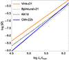 |
Fig. 1. Mass-loss rate as a function of the stellar luminosity at Z = 0.002, according to different wind prescriptions. |
2.2. Other parameters
Besides the upgrade of the mass-loss recipe for OB winds during the main sequence, the other physical ingredients for our evolution models are the same as those implemented by Georgy et al. (2013). This includes initial rotation, vrot/vcrit = 0.4; mass-loss correction due to rotation following Maeder & Meynet (2000); abundances from Asplund et al. (2005, 2009); opacities from Iglesias & Rogers (1996); and an overshooting parameter of αov = 0.1. Angular momentum transport is described by Zahn (1992), with the coefficient Deff for the combined horizontal diffusion and meridional currents taken from Chaboyer & Zahn (1992) and the Dshear coefficient for shear turbulence determined by Maeder (1997). Convective boundaries follow the Schwarzschild criterion. We keep these structures to concentrate our analysis on the differences in mass loss over the main sequence only, regardless of studies suggesting larger overshooting values or Tayler-Spruit for the angular momentum transport (see, i.e. Romagnolo et al. 2024).
Mass-loss recipes outside the range of validity of our Ṁsc (i.e. for Teff < 30 kK and log g < 3.0) are the same as those used by Georgy et al. (2013); they are the same as those used by Vink et al. (2001) for Teff ≥ 10 kK and those of de Jager et al. (1988) for Teff < 10 kK. For WR winds (Xsurf ≤ 0.3 and Teff > 10 kK), we use the formula from Nugis & Lamers (2000).
3. Results
The tracks for our new evolution models adopting self-consistent mass-loss rates at Z = 0.002, compared with models adopting old winds from Georgy et al. (2013), are shown in Fig. 2. The evolution of the mass-loss rates and the stellar radius, comparing Ṁsc and ṀVink, are shown in Fig. 3. The evolution of the rotational velocities is shown in Fig. 4. Table 1 summarises the stellar properties at the end of the main sequence (H-core burning) stage, whereas Table 2 summarises the properties at the end of He-core and C-core burning stages.
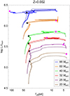 |
Fig. 2. Tracks across HR diagram for evolution models adopting Msc (solid lines), compared with tracks adopting MVink from Georgy et al. (2013; dashed lines). New wind prescription gives values for Ṁ around ∼2 − 6 times lower than the mass-loss adopted for old models, as visualised in Fig. 3. Black stars mark the end of the H-core burning stage, whereas magenta stars mark the end of the He-core burning stage. |
Properties of our selected evolutionary tracks at the end of the H-core burning stage.
Properties of our selected evolutionary tracks at the end of the He-core and C-core burning stage.
3.1. Evolution through the main sequence
Figure 3 shows that the differences between the mass-loss recipes are narrower for the most massive and luminous stellar models. According to Eq. (2), at Z = 0.002 (=0.14 Z⊙) the difference between Ṁsc and ṀVink is only ∼0.05 for our 85 M⊙ model, whereas for our 20 M⊙ model the starting Ṁsc is ∼6.25 times lower than ṀVink (∼0.8 dex), which is also seen for the non-rotating models at Z = 0.002 (Gormaz-Matamala et al. 2022b). However, even though the comparative difference in Ṁ is smaller for our most massive models (60 and 85 M⊙), the upgrade in the mass-loss rate still has an important impact over their evolutionary tracks because their values are the highest in absolute terms (≳2 × 10⁻⁷ M⊙ yr−1). Such an impact is the same as that observed in Gormaz-Matamala et al. (2023), but on a minor scale: weaker wind makes the star rotate faster (Fig. 4), whereas it keeps more of its envelope, which results in a drift redwards in the HR diagram because the inner structure is less homogeneous. Homogeneous chemical composition in the inner stellar structure favours bluewards evolution, as demonstrated by Maeder (1987). Consequently, for new evolution models we find a larger rotational speed during all their MS lifetime, but particularly at the end of it, and a more moderate change in the surface abundances in comparison with old tracks (Table 1).
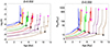 |
Fig. 3. Evolution of mass-loss rates (left panel) and stellar radius (right panel) as function of time, for our new Ṁsc prescription (solid lines) and for ṀVink (dashed lines). The legends for the colours and the black and magenta stars are the same as for Fig. 2. |
On the other side, for the less massive models, comparative differences in the Ṁ recipe are larger but the absolute magnitude of it is smaller (≲2 × 10⁻⁸ M⊙ yr−1). So this time the impact over the stellar evolution is minimal, at least during most of the main sequence. Still, in this case the weaker wind makes the star stay in the MS almost 12% longer for our 25 M⊙ model, and about 14% longer for our 20 M⊙ model. As a consequence, changes in the final surface abundances at the end of H-core burning are larger for the new evolution models adopting weaker winds, because envelope removal becomes negligible and then the changes in the surface composition are preponderantly influenced by the rotational mixing (Maeder & Meynet 2000, 2010).
The MS lifetime is enhanced for our models with Mzams = 20, 25, 32, and (though on a minor scale) 40 M⊙. These are also the models ending their H-core burning stages with the highest rotational velocities, at over 200 km s−1 and with angular momentum of Ω/Ωcrit ≳ 0.7 according to Table 1 and Fig. 4. Although in our case we are just analysing Z = 0.002, this trend agrees with Szécsi et al. (2015) and Kubátová et al. (2019), where stars at low metallicities keep faster rotations due to their weaker winds. Because of this rapid rotation, the inner rotational mixing is strong enough to add more hydrogen to the convective core, thus making the stellar core have more fuel to burn and therefore extend the H-core burning lifetime. Indeed, in Fig. 5 we can see how the hydrogen abundance in the core is ‘bumped’ prior to its total depletion for our new evolution models. The same behaviour is illustrated in more detail in Fig. 6, which shows Kippenhahn diagrams for our six stars covering their MS lifetimes. These bumps in the core hydrogen abundance coincide with the increase in the size of the convective core, meaning that the core gains fuel to extend the H-burning process. The exceptions for this phenomenon are the most massive cases, 60 and 85 M⊙, where the mass loss is strong enough to brake the star prior to the end of H-core burning, and therefore the inner mixing does not refill the convective core.
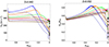 |
Fig. 4. Evolution of rotational velocity expressed as absolute magnitude vrot (left panel) and angular velocity as fraction of the critical velocity Ω/Ωcrit (right panel). New models exhibit larger velocities because they lose less angular momentum due to weaker winds. The legends for the colours and the black stars are the same as for Figs. 2 and 3. |
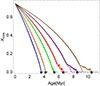 |
Fig. 5. Evolution of hydrogen mass fraction at core, showing extension of MS lifetime for our less massive models. The legends for the colours and the black stars are the same as for previous figures. |
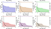 |
Fig. 6. Kippenhahn diagrams, showing evolution of stellar total mass and core mass, for our studied range of masses. Solid coloured lines and shadowed areas represent models adopting new self-consistent winds, whereas grey dashed lines and shadowed areas represent models adopting old winds. Black tracks correspond to the percentage of hydrogen mass fraction in the core. |
The new mass-loss-rate recipe has direct and indirect impacts on the stellar evolution, depending on the initial stellar mass. The impact over the stellar evolution at SMC is direct for the most massive stars (60 and 85 M⊙), because weaker winds remove less material from the outer stellar envelope, thus favouring a less homogeneous structure and, subsequently, a more redwards evolution. On the other side, for the less massive stars of our grid the impact is indirect, and it is observed by means of a more efficient mixing due to a more rapid rotation and a more extended MS lifetime. The contrast between both direct and indirect impacts, which is actually the struggle between mass loss and rotational mixing as the dominant factor driving the evolution of massive stars, is particularly evident in the resulting chemical enrichment at the stellar surface. Differences in the resulting CNO abundances at the stellar surfaces are shown in Table 1 and the N/C and N/O ratios are plotted in Fig. 7, where it is straightforward to observe the contrast in the effects for the most and the least massive models. The changes in the N/C are more drastic than the N/O ratio due to the conditions of the CNO-cycle (Maeder et al. 2014).
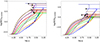 |
Fig. 7. Evolution of ratios of abundance fractions N/C (left panel) and N/O (right panel). The legends for the colours and the black crosses are the same as for previous figures. |
More massive models do not substantially change their MS lifetimes, but the final mixing at the surface is reduced (compared with older evolution models) because weaker winds remove less envelope. Also, the evolution redwards observed for 60 and 85 M⊙ models implies larger radii and thus lower surface gravity. As a consequence, for our new models the log g goes down to ∼3.3 before the final contraction prior to the end of the H-core burning stage, and the final N/C and N/O ratios are lower. On the contrary, for the less massive stars of our model grid (20 and 25 M⊙), the N/C and N/O barely change as the surface gravity decreases, but because less massive models have more extended MS lifetimes and consequently larger final surface mixings, the abundance of nitrogen continues growing until it exceeds the final enrichment shown by the old models. In the middle, we have the 40 M⊙ and the 32 M⊙ models, as moderate versions of both previous effects. The combination of these effects makes our evolutionary tracks to cover wider areas on the planes N/C and N/O-vs.-log g and (Fig. 7), showing these plots the biggest differences between old and new winds.
In summary, new evolution models adopting our self-consistent recipe enhance the influence of the rotational mixing on the surface chemical enrichment, to the detriment of the influence of the mass loss, which is a logical consequence of their lower Ṁ values. In particular for ZSMC = 0.002, the stellar mass showing the lowest N/C ratio is around 40 M⊙ for both old and new winds. Over and below that mass, either mass loss or rotational mixing, respectively, increases nitrogen enrichment (Bouret et al. 2021). However, for the case of N/O we observe that the lowest enrichment ratio belongs to the model with 20 M⊙ adopting old mass-loss recipe (Georgy et al. 2013) and to the model with 40 M⊙ adopting new recipe.
3.2. Evolution through later stages
Beyond the main sequence, for He-core and C-core burning stages, mass loss is described by the same recipes implemented by the models of Georgy et al. (2013): Vink’s formula if Xs ≥ 0.3, or Gräfener & Hamann (2008) if Xsc ≤ 0.3. However, because the changes in the MS mass-loss recipes lead to evolution models finishing their H-core burning stages at different locations of the HRD and with different rotational and chemical properties, their subsequent evolution will retain important differences.
Table 2 summarises the final properties of our evolution models at the end of He-core and C-core burning compared with the models of Georgy et al. (2013). Here again, the contrast between the models dominated by mass loss and the models dominated by rotational mixing becomes even stronger. For our masses 20, 25, and 32 M⊙, which were the models whose MS lifetime was extended and more chemically evolved at the end of H-core burning, the final masses are smaller than their counterpart models adopting old winds. This is due to the fact that these models expand redwards with larger luminosities and larger rotation, thus with larger mass-loss rates, also implying that the CNO mixing at the surface is more enhanced. These effects are less relevant for our 40 M⊙ model, where the final abundances at the end of the MS changed less when we adopted the new winds. In all of these four cases, the stars continue their expansion post-MS even after the end of their He-core burning stages, which is the reason why their largest radii are found during the C-core burning stage when these stars become RSGs. The RSGs predicted by our 25–40 M⊙ models satisfy log L*/L⊙ ≲ 5.7, and they are thus in agreement with the empirical results from Davies et al. (2018), where no RSGs have been found for higher luminosities. The maximum radial expansion of these RSGs is barely affected (only our 20 M⊙ increases its maximum radius by ∼100 R⊙), thus causing Rmax to grow with mass from ∼900 R⊙ at Mzams = 20 M⊙ to ∼1280 R⊙ at Mzams = 40 M⊙. That maximum radial expansion (for all our masses) lies close to the ∼1300 R⊙ found for the RSG Dachs SMC 1–4 (the largest star known in the SMC; Gilkis et al. 2021), but its determined luminosity log LDachsSMC1 − −4/L⊙ ≃ 5.55 does not coincide with the luminosity predicted by our 40 M⊙ model (L*/L⊙ ≃ 5.7). This reinforces that, besides the mass-loss upgrade, evolution models need to revise the convection treatment for the inner layers, given that a less efficient semi-convective mixing extends the band on the HRD where RSGs can exist (Schootemeijer et al. 2019). The luminosity of red supergiants (RSGs) is also important, because it is directly correlated with the MHe, core prior to the core-collapse supernovae (Farrell et al. 2020).
On the other side, our 60 and 85 M⊙ models end the H-core burning stage with more mass and a less chemically evolved surface (compared with models for the same masses adopting old winds) prior to the post-MS expansion. Because they also reach the end of the radial expansion with larger masses (i.e. when they reach Teff ≤ 9 kK and then return bluewards), they experience a mass loss large enough to revert the previous scenario and then end their He-core burning stages with smaller masses. We remind the reader that, for these stars, Ṁ ≳ 10−6 M⊙ yr−1, and therefore the discrepancies in mass loss create a stronger impact. For the case of our 60 M⊙ model, this extra mass loss during the He-core burning is expressed not only in a smaller final mass but also in larger N/C and N/O ratios as consequence of the extra removal of envelope. The case of our 85 M⊙ model is even more extreme, because this extra removal includes the latest envelopes of hydrogen; therefore, the star becomes a Wolf-Rayet, thus following a completely different track compared to the corresponding model adopting old wind recipe. Namely, larger temperatures and a CNO mass fraction of ∼40%, with reduced N/C and N/O ratios (Table 2), occur because surface nitrogen has been quickly removed. In other words, the adoption of self-consistent winds for Ṁ reduces the threshold on Mzams, over the which stars are expected to become WR at Z = 0.002. This is important because it implies that new evolution models might have a better match with the WR stars at SMC studied by Hainich et al. (2015), which could not be reproduced by the evolution models of Georgy et al. (2013). Nevertheless, we need to upgrade the Ṁ recipe not only for OB-type stars’ optically thin winds, but also for the WR optically thick winds (Bestenlehner 2020; Sander & Vink 2020; Sander et al. 2023), as well as revisiting the criteria for the transition between these wind regimes (which depends more on the proximity to the Eddington limit than on the surface hydrogen abundance, as asserted by Gräfener 2021) before a more robust prediction for WR stars can be performed.
We reiterate that the mass-loss recipes adopted during the He-core burning stage are the same as in Georgy et al. (2013), because self-consistent m-CAK prescription only works for Teff ≥ 30 kK. Henceforth, the described differences between old and new evolution models stem from the models ending the H-core burning stage with different masses and chemical abundances at the surface. This reinforces the importance of upgrading mass-loss formulae for massive stars during their main sequence, specially because our self-consistent Ṁ is ∼2 − 6 times lower than the formula from Vink et al. (2001) originally adopted for the SMC evolution models.
4. Observational diagnostics
We compare the predicted stellar evolution for massive stars at SMC metallicity with the observational diagnostics performed Bouret et al. (2021) for O-type giants and supergiants. We do not include O-dwarves from Bouret et al. (2013), because they are in a very early stage of the main sequence, where the differences between old and new evolution models are barely perceptible. Despite the most remarkable differences between tracks adopting either old or new winds are observed for the N/C and N/O ratios as seen in Fig. 7, we do not include these diagnostics in this section because determining the baseline CNO abundances in the SMC is not a trivial task. By default, our evolution models use the abundances given by Asplund et al. (2009) rescaled to Z = 0.002 (=0.14 Z⊙). However, different studies applying different tracers such as B-type stars (Rolleston et al. 2003; Hunter et al. 2009; Dufton et al. 2020) or supernova remnants (Dopita et al. 2019) have determined distinct initial values for N/C and N/O ratios, thus making impossible to set a reliable baseline for CNO abundances in the SMC. Therefore, we concentrate our analysis and discussion of chemical evolution on the N/H ratio.
By taking the effective temperatures and surface gravities, we readapt our evolutionary tracks to the spectroscopic HR diagram (sHRD), which is analogous to the original HR diagram, but shows a plane of Teff versus  instead of the luminosity L* (Langer & Kudritzki 2014). The main advantage of the sHRD is that both quantities, effective temperature and surface gravity, are spectroscopically determined and distance independent, which is particularly important for the study of sources in other galaxies. For the analysis of the chemical enrichment we provide Hunter diagrams (Hunter et al. 2009), which relate nitrogen over hydrogen abundance (by number) to the projected rotational velocity (v sin i). The selected stars, together with their parameters determined by Bouret et al. (2021), are shown in Table 3.
O-type giants and supergiants from Bouret et al. (2021).
The results for both diagrams are shown in Fig. 8. Because the evolutionary stages of O-type giants and supergiants correspond either to the late H-core burning stage or the beginning of the He-core burning stage, the helium at the surface shown in Table 1 is comparable with the helium-mass fractions shown in Table 3. Therefore, the helium-mass fraction can help us to expand our comparison between old and new models, especially if we consider the large uncertainties in our analysed stellar sample. Hence, we observe that for AV 439, whose high rotational speed suggests that it is still in the MS, shows a better agreement with both the nitrogen enrichment and the surface helium predicted by our new 20 M⊙ evolution model. This is because its YHe = 0.308 lies below the final value expected at the end of the H-core burning stage. Indeed, an old 20 M⊙ model would never reach such a helium-mass fraction, not even beyond the H-core burning stage, as shown in Table 2. Likewise, stars AV 307 and AV 43 are also located in the Hertzsprung gap of the old 20 M⊙ evolution model and show good agreement with respect to the expected nitrogen enrichment; however, their large helium-mass fractions (YHe = 0.324 and 0.374, respectively) match better with the predicted Ysurf by the new 20 M⊙ model. Similar conclusions can be deduced for the other stars; for example, AV 15 (Teff = 39.0 kK, log g = 3.61) matches to our 60 M⊙ (during H-core burning) and 40 M⊙ (end of H-core burning) models, but its poor helium enrichment (YHe = 0.285) suggests that the 60 M⊙ scenario is more realistic. The same is the case for AV 95 (Teff = 38.0 kK, log g = 3.7), which matches the MS bands of the models with 40 and 32 M⊙ with its YHe = 0.285.
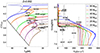 |
Fig. 8. Comparison of old and new evolution models, with respect to the sample of SMC evolved stars from Bouret et al. (2021): AV 15, AV 43, AV 47, AV 69, AV 75, AV 77, AV 83, AV 95, AV 170, AV 232, AV 307, AV 327, and AV 439. Left panel: spectroscopic HR diagram showing Teff vs. |

For the stars showing larger nitrogen enrichments, AV 75 (Teff = 38.5 kK, log g = 3.51) shows a match with our 85 M⊙ – in line with its MS position in the s-HRD – thus suggesting this star was born with a larger initial mass. On the other hand, AV 327 (Teff = 30 kK, log g = 3.12) also shows a large nitrogen enrichment, but this is not in line with its position in the s-HRD; however, its helium enrichment (YHe = 0.374) agrees with the predictions of the new models as well. The only two stars whose larger nitrogen abundances do not match with any of the new tracks in the Hunter diagram are AV 232 and AV 83, which are also the stars with the largest mass fraction of helium at the surface (YHe = 0.444), thus suggesting that these stars were also fast rotators at the beginning of their lives, in agreement with Hillier et al. (2003).
The other extremely poorly nitrogen-enriched stars are AV 77, AV 47, and AV 69. These first two stars are located in the MS band of the sHRD, but only AV 47 shows a helium-mass fraction (YHe = 0.285) below that expected at the end of the H-core burning for old and new 25 M⊙ models. Because of its age of ∼6 Myr, its lower nitrogen abundance might be a product of it being a slow rotator (v sin i = 60) in the last part of its MS lifetime. For the case of AV 77, evidence of binarity is detected in its spectrum (Bouret et al. 2021), and then more information about its companion is required to adequately describe the evolutionary status of the star. The most extreme case of a poorly nitrogen-enriched star is AV 69 (even lying out of the plot range of Fig. 8). The deficient nitrogen abundance of AV 69 is even below the baseline N abundances assumed for the SMC, thus suggesting that this star is a slow rotator with negligible mixing (Hillier et al. 2003). On a minor scale, a slightly lower rotation could explain the abundances of AV 170, which is located in the Hertzsprung gap of our 25 M⊙ model, but its Ysurf = 0.324 lies marginally below the predicted by new models (but still above the predictions of old models). Therefore, our new evolution models can describe the observed properties of O-type stars at metallicity Z = 0.002, with the natural exception of fast and slow rotators (i.e. both with vini/vrot ≠ 0.4) and binary stars.
In synthesis, evolution models adopting weaker winds for the main sequence not only modify the predicted tracks over the HR and sHR diagrams, but also the chemical diagnostics expected for massive stars, especially at the end of the MS. For this reason, the most optimal observational data to use in our diagnostics corresponds to stars at ‘evolved’ stages such as O-giants and supergiants rather than ‘unevolved’ O-dwarves. We can conclude a different evolutionary status for the evolved O-type stars from Bouret et al. (2021) based on our new models, notwithstanding that such conclusions cannot be the final word, because the analysed sample contains only 13 stars and because the observational uncertainties are still significant. We expect to be able to draw stronger conclusions in the near future thanks to upcoming projects such as XShootU (Vink et al. 2023; Hawcroft et al. 2024), also exploring other spectroscopic phases such as BSGs (Bernini-Peron et al., in prep.) and even RSGs if possible.
5. Summary and conclusions
This work is an extension of the previous evolution studies from Gormaz-Matamala et al. (2022b); Gormaz-Matamala et al. (2023), in which we upgraded the mass-loss formula for the winds of massive stars adopting the m-CAK prescription (Gormaz-Matamala et al. 2019, 2022a) and a lower metallicity. Here, we studied the impact in a low-metallicity environment, the SMC (Z = 0.002), where the overall mass loss is weaker. In concordance, we observe that the most significant repercussion of new winds (which range from ∼2 − 6 times weaker than old winds) is not given by the amount of removed mass (as it happens for more massive scenarios at higher metallicities), but by the level of chemical evolution observed at the stellar surface. These divergences in chemical evolution are due to weaker winds causing stars to lose less angular momentum and therefore keeping a fast rotational speed for a prolonged time, thus producing a more efficient rotational mixing.
For our 20–40 M⊙ models, stars end their H-core burning stage more chemically evolved when new winds are adopted, whereas 60 and 85 M⊙ models end with less chemically evolved surfaces. These results are important for spectroscopical diagnostics, especially those that provide values for He and CNO abundances of massive stars in the SMC. However, the accuracy of such diagnostics depends not only on the quality of spectra but also on the evolutionary stage of the sources. O-dwarves from Bouret et al. (2013) are too young to use for a comparison between old and new evolution models, whereas O-giants and supergiants from Bouret et al. (2021) could give us more insight if we exclude fast rotators and slow rotators. Notwithstanding this, analyses of chemical evolution need to be extended to latter spectroscopic stages such as BSG and RSG stages. Concerning BSG, new values for He and CNO abundances have been obtained thanks to the XShootU project (Bernini-Peron et al., in prep.). On the same subject, we are preparing extensions of evolution models covering the He-core burning stage for Galactic and LMC metallicities to compare with the BSG properties found by Bernini-Peron et al. (2023). Concerning RSGs, they are important to explore because they reach the largest stellar expansion, which is a key factor for the evolution of close binaries as it affects mass transfer interactions and, in turn, the formation of GW sources (Romagnolo et al. 2023). Upgrades on the line-driven wind recipes barely modify the Rmax values, thus suggesting that other features such as core overshooting and semi-convection also need to be upgraded (Schootemeijer et al. 2019; Martinet et al. 2021; Gilkis et al. 2021), not to mention the most recent studies about the dust-driven winds for RSGs (Beasor et al. 2020; Kee et al. 2021; Decin et al. 2024), which replace the old Ṁ prescription from de Jager et al. (1988).
The mass-loss formulae adopted for our evolution models from 20 to 40 M⊙ are the state-of-the-art, whereas the models for 60 and 85 exposed in this work have the purpose of compare the effect of new winds during main sequence but they still need to update mass-loss recipe for later stages. The new recipes for WR stars from Sander et al. (2020) and Sander & Vink (2020), together with thick winds in the proximity to the Eddington factor (Gräfener et al. 2011; Bestenlehner 2020), are beyond the scope of this paper.
The results of this work highlight the importance of upgrading the mass-loss prescriptions in the study of the evolution of massive stars, in particular for their earlier evolutionary stages, even for low-metallicity environments where the removed mass during the stellar lifetime is expected to be modest. The upgrades introduced in Gormaz-Matamala et al. (2022b); Gormaz-Matamala et al. (2023) and here, however, represent the current state-of-the-art related to stellar winds, but they do not provide the definitive answer concerning stellar evolution. These studies needs to be complemented by upgrades in other aspects of the stellar structure, such as the convective core overshooting (Martinet et al. 2021; Scott et al. 2021; Baraffe et al. 2023), the revision of the initial rotational velocities to be adopted, and, naturally, the upgrading of the mass-loss formula for the advanced stages such as those of RSGs and WRs. These features play a major role for more massive stars, which will be explored in more detail in a forthcoming work.
Vink’s formula is defined as
![Mathematical equation: $$ \begin{aligned}&\log \dot{M}_{\rm Vink}=C_1+C_2\log \left(\frac{L_*}{10^5L_\odot }\right)+C_3\log \left(\frac{M_*}{30M_\odot }\right)+C_4\log \left(\frac{v_\infty }{2v_{\rm esc}}\right)\nonumber \\&\qquad \qquad +C_5\log \left(\frac{T_{\rm eff}}{20\,\mathrm{kK}}\right)-C_6\left[\log \left(\frac{T_{\rm eff}}{40\,\mathrm{kK}}\right)\right]^2+0.85\log (Z_*/Z_\odot ).\nonumber \end{aligned} $$](/articles/aa/full_html/2024/07/aa49782-24/aa49782-24-eq24.gif)
Where the constants C1, C2, C3, C4, C5, and C6 have different values depending on which temperature range the formula is evaluated in.
Acknowledgments
We thank to the anonymous referee for their valuable comments. ACGM acknowledges the support from the Polish National Science Centre grant Maestro (2018/30/A/ST9/00050). ACGM and JC acknowledge the support from the Max Planck Society through a “Partner Group” grant. JC acknowledges financial support from FONDECYT Regular 1211429. GM and SE has received funding from the European Research Council (ERC) under the European Union’s Horizon 2020 research and innovation programme (grant agreement N° 833925, project STAREX). SE also acknowledges the support from the Swiss National Science Foundation (SNSF). MC acknowledges the support from Centro de Astrofísica de Valparaíso, Chile, and is also grateful the support from FONDECYT project 1230131. We dedicate this paper to Prof. Krzysztof Belczynski, who contributed to this research before his untimely passing on the 13th of January 2024.
References
- Abbott, D. C. 1982, ApJ, 259, 282 [Google Scholar]
- Abbott, R., Abbott, T. D., Abraham, S., et al. 2021, ApJ, 913, L7 [NASA ADS] [CrossRef] [Google Scholar]
- Agrawal, P., Stevenson, S., Szécsi, D., & Hurley, J. 2022, A&A, 668, A90 [NASA ADS] [CrossRef] [EDP Sciences] [Google Scholar]
- Asplund, M., Grevesse, N., & Sauval, A. J. 2005, in Cosmic Abundances as Records of Stellar Evolution and Nucleosynthesis, eds. I. Barnes, G. Thomas, & F. N. Bash, ASP Conf. Ser., 336, 25 [NASA ADS] [Google Scholar]
- Asplund, M., Grevesse, N., Sauval, A. J., & Scott, P. 2009, ARA&A, 47, 481 [NASA ADS] [CrossRef] [Google Scholar]
- Baraffe, I., Clarke, J., Morison, A., et al. 2023, MNRAS, 519, 5333 [NASA ADS] [CrossRef] [Google Scholar]
- Bavera, S. S., Fragos, T., Zapartas, E., et al. 2023, Nat. Astron., 7, 1090 [NASA ADS] [CrossRef] [Google Scholar]
- Beasor, E. R., Davies, B., Smith, N., et al. 2020, MNRAS, 492, 5994 [Google Scholar]
- Belczynski, K., Bulik, T., Fryer, C. L., et al. 2010, ApJ, 714, 1217 [NASA ADS] [CrossRef] [Google Scholar]
- Bernini-Peron, M., Marcolino, W. L. F., Sander, A. A. C., et al. 2023, A&A, 677, A50 [NASA ADS] [CrossRef] [EDP Sciences] [Google Scholar]
- Bestenlehner, J. M. 2020, MNRAS, 493, 3938 [Google Scholar]
- Björklund, R., Sundqvist, J. O., Puls, J., & Najarro, F. 2021, A&A, 648, A36 [EDP Sciences] [Google Scholar]
- Björklund, R., Sundqvist, J. O., Singh, S. M., Puls, J., & Najarro, F. 2023, A&A, 676, A109 [NASA ADS] [CrossRef] [EDP Sciences] [Google Scholar]
- Bouret, J. C., Lanz, T., & Hillier, D. J. 2005, A&A, 438, 301 [NASA ADS] [CrossRef] [EDP Sciences] [Google Scholar]
- Bouret, J. C., Hillier, D. J., Lanz, T., & Fullerton, A. W. 2012, A&A, 544, A67 [NASA ADS] [CrossRef] [EDP Sciences] [Google Scholar]
- Bouret, J. C., Lanz, T., Martins, F., et al. 2013, A&A, 555, A1 [NASA ADS] [CrossRef] [EDP Sciences] [Google Scholar]
- Bouret, J. C., Martins, F., Hillier, D. J., et al. 2021, A&A, 647, A134 [NASA ADS] [CrossRef] [EDP Sciences] [Google Scholar]
- Castor, J. I., Abbott, D. C., & Klein, R. I. 1975, ApJ, 195, 157 [Google Scholar]
- Chaboyer, B., & Zahn, J. P. 1992, A&A, 253, 173 [NASA ADS] [Google Scholar]
- Curé, M. 2004, ApJ, 614, 929 [CrossRef] [Google Scholar]
- Curé, M., & Rial, D. F. 2007, Astron. Nachr., 328, 513 [CrossRef] [Google Scholar]
- Davies, B., Crowther, P. A., & Beasor, E. R. 2018, MNRAS, 478, 3138 [NASA ADS] [CrossRef] [Google Scholar]
- Decin, L., Richards, A. M. S., Marchant, P., & Sana, H. 2024, A&A, 681, A17 [NASA ADS] [CrossRef] [EDP Sciences] [Google Scholar]
- de Jager, C., Nieuwenhuijzen, H., & van der Hucht, K. A. 1988, A&AS, 72, 259 [NASA ADS] [Google Scholar]
- Dopita, M. A., Seitenzahl, I. R., Sutherland, R. S., et al. 2019, AJ, 157, 50 [Google Scholar]
- Driessen, F. A., Sundqvist, J. O., & Kee, N. D. 2019, A&A, 631, A172 [NASA ADS] [CrossRef] [EDP Sciences] [Google Scholar]
- Driessen, F. A., Sundqvist, J. O., & Dagore, A. 2022, A&A, 663, A40 [NASA ADS] [CrossRef] [EDP Sciences] [Google Scholar]
- Dufton, P. L., Evans, C. J., Lennon, D. J., & Hunter, I. 2020, A&A, 634, A6 [NASA ADS] [CrossRef] [EDP Sciences] [Google Scholar]
- Eggenberger, P., Meynet, G., Maeder, A., et al. 2008, Ap&SS, 316, 43 [Google Scholar]
- Farrell, E. J., Groh, J. H., Meynet, G., & Eldridge, J. J. 2020, MNRAS, 494, L53 [NASA ADS] [CrossRef] [Google Scholar]
- Georgy, C., Ekström, S., Eggenberger, P., et al. 2013, A&A, 558, A103 [NASA ADS] [CrossRef] [EDP Sciences] [Google Scholar]
- Gilkis, A., Shenar, T., Ramachandran, V., et al. 2021, MNRAS, 503, 1884 [NASA ADS] [CrossRef] [Google Scholar]
- Gormaz-Matamala, A. C., Curé, M., Cidale, L. S., & Venero, R. O. J. 2019, ApJ, 873, 131 [NASA ADS] [CrossRef] [Google Scholar]
- Gormaz-Matamala, A. C., Curé, M., Hillier, D. J., et al. 2021, ApJ, 920, 64 [NASA ADS] [CrossRef] [Google Scholar]
- Gormaz-Matamala, A. C., Curé, M., Lobel, A., et al. 2022a, A&A, 661, A51 [NASA ADS] [CrossRef] [EDP Sciences] [Google Scholar]
- Gormaz-Matamala, A. C., Curé, M., Meynet, G., et al. 2022b, A&A, 665, A133 [NASA ADS] [CrossRef] [EDP Sciences] [Google Scholar]
- Gormaz-Matamala, A. C., Cuadra, J., Meynet, G., & Curé, M. 2023, A&A, 673, A109 [NASA ADS] [CrossRef] [EDP Sciences] [Google Scholar]
- Gräfener, G. 2021, A&A, 647, A13 [NASA ADS] [CrossRef] [EDP Sciences] [Google Scholar]
- Gräfener, G., & Hamann, W. R. 2008, A&A, 482, 945 [Google Scholar]
- Gräfener, G., Vink, J. S., de Koter, A., & Langer, N. 2011, A&A, 535, A56 [NASA ADS] [CrossRef] [EDP Sciences] [Google Scholar]
- Hainich, R., Pasemann, D., Todt, H., et al. 2015, A&A, 581, A21 [NASA ADS] [CrossRef] [EDP Sciences] [Google Scholar]
- Hawcroft, C., Sana, H., Mahy, L., et al. 2021, A&A, 655, A67 [NASA ADS] [CrossRef] [EDP Sciences] [Google Scholar]
- Hawcroft, C., Sana, H., Mahy, L., et al. 2024, A&A, in press, http://dx.doi.org/10.1051/0004-6361/202245588 [Google Scholar]
- Heger, A., Fryer, C. L., Woosley, S. E., Langer, N., & Hartmann, D. H. 2003, ApJ, 591, 288 [CrossRef] [Google Scholar]
- Hillier, D. J., Lanz, T., Heap, S. R., et al. 2003, ApJ, 588, 1039 [Google Scholar]
- Holgado, G., Simón-Díaz, S., Herrero, A., & Barbá, R. H. 2022, A&A, 665, A150 [NASA ADS] [CrossRef] [EDP Sciences] [Google Scholar]
- Hunter, I., Brott, I., Langer, N., et al. 2009, A&A, 496, 841 [NASA ADS] [CrossRef] [EDP Sciences] [Google Scholar]
- Iglesias, C. A., & Rogers, F. J. 1996, ApJ, 464, 943 [NASA ADS] [CrossRef] [Google Scholar]
- Kee, N. D., Sundqvist, J. O., Decin, L., de Koter, A., & Sana, H. 2021, A&A, 646, A180 [NASA ADS] [CrossRef] [EDP Sciences] [Google Scholar]
- Keszthelyi, Z., Puls, J., & Wade, G. A. 2017, A&A, 598, A4 [NASA ADS] [CrossRef] [EDP Sciences] [Google Scholar]
- Krtička, J., & Kubát, J. 2017, A&A, 606, A31 [NASA ADS] [CrossRef] [EDP Sciences] [Google Scholar]
- Krtička, J., & Kubát, J. 2018, A&A, 612, A20 [NASA ADS] [CrossRef] [EDP Sciences] [Google Scholar]
- Kubátová, B., Szécsi, D., Sander, A. A. C., et al. 2019, A&A, 623, A8 [NASA ADS] [CrossRef] [EDP Sciences] [Google Scholar]
- Langer, N., & Kudritzki, R. P. 2014, A&A, 564, A52 [NASA ADS] [CrossRef] [EDP Sciences] [Google Scholar]
- Maeder, A. 1987, A&A, 178, 159 [NASA ADS] [Google Scholar]
- Maeder, A. 1997, A&A, 321, 134 [NASA ADS] [Google Scholar]
- Maeder, A., & Meynet, G. 2000, A&A, 361, 159 [NASA ADS] [Google Scholar]
- Maeder, A., & Meynet, G. 2010, New A Rev., 54, 32 [NASA ADS] [CrossRef] [Google Scholar]
- Maeder, A., Przybilla, N., Nieva, M.-F., et al. 2014, A&A, 565, A39 [NASA ADS] [CrossRef] [EDP Sciences] [Google Scholar]
- Martinet, S., Meynet, G., Ekström, S., et al. 2021, A&A, 648, A126 [NASA ADS] [CrossRef] [EDP Sciences] [Google Scholar]
- Meynet, G., Maeder, A., Schaller, G., Schaerer, D., & Charbonnel, C. 1994, A&AS, 103, 97 [Google Scholar]
- Nugis, T., & Lamers, H. J. G. L. M. 2000, A&A, 360, 227 [NASA ADS] [Google Scholar]
- Olejak, A., & Belczynski, K. 2021, ApJ, 921, L2 [NASA ADS] [CrossRef] [Google Scholar]
- Olejak, A., Belczynski, K., & Ivanova, N. 2021, A&A, 651, A100 [NASA ADS] [CrossRef] [EDP Sciences] [Google Scholar]
- Pauldrach, A., Puls, J., & Kudritzki, R. P. 1986, A&A, 164, 86 [NASA ADS] [Google Scholar]
- Rolleston, W. R. J., Venn, K., Tolstoy, E., & Dufton, P. L. 2003, A&A, 400, 21 [NASA ADS] [CrossRef] [EDP Sciences] [Google Scholar]
- Romagnolo, A., Belczynski, K., Klencki, J., et al. 2023, MNRAS, 525, 706 [NASA ADS] [CrossRef] [Google Scholar]
- Romagnolo, A., Gormaz-Matamala, A. C., & Belczynski, K. 2024, ApJ, 964, L23 [NASA ADS] [CrossRef] [Google Scholar]
- Sander, A. A. C., & Vink, J. S. 2020, MNRAS, 499, 873 [Google Scholar]
- Sander, A. A. C., Hamann, W.-R., Todt, H., Hainich, R., & Shenar, T. 2017, A&A, 603, A86 [NASA ADS] [CrossRef] [EDP Sciences] [Google Scholar]
- Sander, A. A. C., Vink, J. S., & Hamann, W. R. 2020, MNRAS, 491, 4406 [Google Scholar]
- Sander, A. A. C., Lefever, R. R., Poniatowski, L. G., et al. 2023, A&A, 670, A83 [NASA ADS] [CrossRef] [EDP Sciences] [Google Scholar]
- Schootemeijer, A., Langer, N., Grin, N. J., & Wang, C. 2019, A&A, 625, A132 [NASA ADS] [CrossRef] [EDP Sciences] [Google Scholar]
- Scott, L. J. A., Hirschi, R., Georgy, C., et al. 2021, MNRAS, 503, 4208 [NASA ADS] [CrossRef] [Google Scholar]
- Sundqvist, J. O., & Puls, J. 2018, A&A, 619, A59 [NASA ADS] [CrossRef] [EDP Sciences] [Google Scholar]
- Sundqvist, J. O., Björklund, R., Puls, J., & Najarro, F. 2019, A&A, 632, A126 [NASA ADS] [CrossRef] [EDP Sciences] [Google Scholar]
- Szécsi, D., Langer, N., Yoon, S.-C., et al. 2015, A&A, 581, A15 [NASA ADS] [CrossRef] [EDP Sciences] [Google Scholar]
- Vink, J. S., & Sander, A. A. C. 2021, MNRAS, 504, 2051 [NASA ADS] [CrossRef] [Google Scholar]
- Vink, J. S., de Koter, A., & Lamers, H. J. G. L. M. 2001, A&A, 369, 574 [NASA ADS] [CrossRef] [EDP Sciences] [Google Scholar]
- Vink, J. S., Mehner, A., Crowther, P. A., et al. 2023, A&A, 675, A154 [NASA ADS] [CrossRef] [EDP Sciences] [Google Scholar]
- Šurlan, B., Hamann, W. R., Kubát, J., Oskinova, L. M., & Feldmeier, A. 2012, A&A, 541, A37 [NASA ADS] [CrossRef] [EDP Sciences] [Google Scholar]
- Šurlan, B., Hamann, W. R., Aret, A., et al. 2013, A&A, 559, A130 [NASA ADS] [CrossRef] [EDP Sciences] [Google Scholar]
- Zahn, J. P. 1992, A&A, 265, 115 [NASA ADS] [Google Scholar]
All Tables
Properties of our selected evolutionary tracks at the end of the H-core burning stage.
Properties of our selected evolutionary tracks at the end of the He-core and C-core burning stage.
All Figures
|
Fig. 1. Mass-loss rate as a function of the stellar luminosity at Z = 0.002, according to different wind prescriptions. |
| In the text | |
|
Fig. 2. Tracks across HR diagram for evolution models adopting Msc (solid lines), compared with tracks adopting MVink from Georgy et al. (2013; dashed lines). New wind prescription gives values for Ṁ around ∼2 − 6 times lower than the mass-loss adopted for old models, as visualised in Fig. 3. Black stars mark the end of the H-core burning stage, whereas magenta stars mark the end of the He-core burning stage. |
| In the text | |
|
Fig. 3. Evolution of mass-loss rates (left panel) and stellar radius (right panel) as function of time, for our new Ṁsc prescription (solid lines) and for ṀVink (dashed lines). The legends for the colours and the black and magenta stars are the same as for Fig. 2. |
| In the text | |
|
Fig. 4. Evolution of rotational velocity expressed as absolute magnitude vrot (left panel) and angular velocity as fraction of the critical velocity Ω/Ωcrit (right panel). New models exhibit larger velocities because they lose less angular momentum due to weaker winds. The legends for the colours and the black stars are the same as for Figs. 2 and 3. |
| In the text | |
|
Fig. 5. Evolution of hydrogen mass fraction at core, showing extension of MS lifetime for our less massive models. The legends for the colours and the black stars are the same as for previous figures. |
| In the text | |
|
Fig. 6. Kippenhahn diagrams, showing evolution of stellar total mass and core mass, for our studied range of masses. Solid coloured lines and shadowed areas represent models adopting new self-consistent winds, whereas grey dashed lines and shadowed areas represent models adopting old winds. Black tracks correspond to the percentage of hydrogen mass fraction in the core. |
| In the text | |
|
Fig. 7. Evolution of ratios of abundance fractions N/C (left panel) and N/O (right panel). The legends for the colours and the black crosses are the same as for previous figures. |
| In the text | |
|
Fig. 8. Comparison of old and new evolution models, with respect to the sample of SMC evolved stars from Bouret et al. (2021): AV 15, AV 43, AV 47, AV 69, AV 75, AV 77, AV 83, AV 95, AV 170, AV 232, AV 307, AV 327, and AV 439. Left panel: spectroscopic HR diagram showing Teff vs. |
| In the text | |
Current usage metrics show cumulative count of Article Views (full-text article views including HTML views, PDF and ePub downloads, according to the available data) and Abstracts Views on Vision4Press platform.
Data correspond to usage on the plateform after 2015. The current usage metrics is available 48-96 hours after online publication and is updated daily on week days.
Initial download of the metrics may take a while.