| Issue |
A&A
Volume 695, March 2025
|
|
|---|---|---|
| Article Number | A224 | |
| Number of page(s) | 18 | |
| Section | Planets, planetary systems, and small bodies | |
| DOI | https://doi.org/10.1051/0004-6361/202452547 | |
| Published online | 25 March 2025 | |
Water depletion and 15NH3 in the atmosphere of the coldest brown dwarf observed with JWST/MIRI
1
ETH Zürich, Institute for Particle Physics and Astrophysics,
Wolfgang-Pauli-Str. 27,
8093
Zürich, Switzerland
2
Max-Planck-Institut für Astronomie,
Königstuhl 17,
69117
Heidelberg, Germany
3
Université Paris-Saclay, UVSQ, CNRS, CEA, Maison de la Simulation,
91191,
Gif-sur-Yvette, France
4
Department of Astrophysics, American Museum of Natural History,
New York,
NY
10024, USA
5
STAR Institute, Université de Liège, Allée du Six Août 19c,
4000
Liège,
Belgium
6
Centro de Astrobiología (CAB), CSIC-INTA, ESAC Campus,
Camino Bajo del Castillo s/n,
28692
Villanueva de la Cañada, Madrid,
Spain
7
SRON Netherlands Institute for Space Research,
Niels Bohrweg 4,
2333
CA Leiden, The Netherlands
8
Université Paris-Saclay, Université Paris Cité, CEA, CNRS, AIM,
91191
Gif-sur-Yvette, France
9
Department of Astrophysics/IMAPP, Radboud University,
PO Box 9010,
6500
GL Nijmegen, The Netherlands
10
Department of Astrophysics, University of Vienna,
Türkenschanzstr. 17,
1180
Vienna, Austria
11
Institute of Astronomy, KU Leuven,
Celestijnenlaan 200D,
3001
Heverlee,
Belgium
12
LESIA, Observatoire de Paris, Université PSL, CNRS, Sorbonne Université, Université de Paris Cité,
5 place Jules Janssen,
92195
Meudon,
France
13
School of Physics & Astronomy, Space Park Leicester, University of Leicester,
92 Corporation Road,
Leicester
LE4 5SP, UK
14
Leiden Observatory, Leiden University,
PO Box 9513,
2300
RA Leiden, The Netherlands
15
Department of Astronomy, Oskar Klein Centre, Stockholm University,
106
91 Stockholm, Sweden
16
School of Cosmic Physics, Dublin Institute for Advanced Studies,
31 Fitzwilliam Place,
Dublin,
D02 XF86,
Ireland
17
UK Astronomy Technology Centre, Royal Observatory Edinburgh,
Blackford Hill,
Edinburgh
EH9 3HJ, UK
★ Corresponding author; This email address is being protected from spambots. You need JavaScript enabled to view it.
Received:
9
October
2024
Accepted:
19
January
2025
Abstract
Context. With a temperature of ∼285 K, WISEJ0855–0714 (hereafter, WISE 0855) is the coldest brown dwarf observed thus far. Studying such cold gas giants allows us to probe the atmospheric physics and chemistry of evolved objects that resemble Solar System gas giants.
Aims. Using James Webb Space Telescope (JWST), we obtained observations to characterize WISE 0855’s atmosphere, focusing on vertical variation in the water steam abundance, measuring trace gas abundances, and obtaining the bulk parameters for this cold object.
Methods. We observed the ultra-cool dwarf WISE 0855 using the Mid-Infrared Instrument Medium Resolution Spectrometer (MIRI/MRS) on board JWST at a spectral resolution of up to 3750. We combined the observation with published data from the Near-Infrared Spectrograph (NIRSpec) G395M and PRISM modes, yielding a spectrum ranging from 0.8 to 22 µm. We applied atmospheric retrievals using <mono>petitRADTRANS</mono> to measure the atmospheric abundances, pressure-temperature structure, radius, and gravity of the brown dwarf. We also employed publicly available clear and cloudy self-consistent grid models to estimate the bulk properties of the atmosphere such as the effective temperature, radius, gravity, and metallicity.
Results. Atmospheric retrievals have constrained a variable water abundance profile in the atmosphere, as predicted by equilibrium chemistry. We detected the 15NH3 isotopolog and inferred a ratio of volume fraction of 14NH3/15 NH3 = 349−41+53 for the clear retrieval. We measured the bolometric luminosity by integrating the presented spectrum, obtaining a value of log(L/L⊙) = −7.291 ± 0.008.
Conclusions. The detected water depletion indicates that water condenses out in the upper atmosphere due to the very low effective temperature of WISE 0855. The height in the atmosphere where this occurs is covered by the MIRI/MRS data, thereby demonstrating the potential of MIRI to characterize the atmospheres of cold gas giants. After comparing the data to retrievals and self-consistent grid models, we did not detect any signs of water ice clouds, although their spectral features have been predicted in previous studies.
Key words: instrumentation: spectrographs / methods: observational / planets and satellites: atmospheres / stars: atmospheres / brown dwarfs
© The Authors 2025
 Open Access article, published by EDP Sciences, under the terms of the Creative Commons Attribution License (https://creativecommons.org/licenses/by/4.0), which permits unrestricted use, distribution, and reproduction in any medium, provided the original work is properly cited.
This article is published in open access under the Subscribe to Open model. This email address is being protected from spambots. You need JavaScript enabled to view it. to support open access publication.
1 Introduction
Y dwarfs are characterized by cold temperatures below 500 K (Cushing et al. 2011). As they are often either far from their host star or free-floating, they are prime targets for spectroscopic characterization with direct imaging. Their atmospheres are comparable to gas giant’s atmospheres in terms of their temperature and composition (Burrows et al. 1997; Beichman et al. 2014). In addition, they can be used to characterize evolved atmospheres and investigate the formation of weather patters and clouds similar to the processes in Jupiter in the Solar System (Coulter et al. 2022). For the first time, the James Webb Space Telescope (JWST; Gardner et al. 2023; Rigby et al. 2023) has enabled the measurement and characterization of such cold objects in the mid-infrared (MIR). Barrado et al. (2023) presented the first detection of the ammonia isotopolog15 NH3 in the Y dwarf WISEPA J182831.08+265037.8 (hereafter, WISE 1828). In the near-infrared (NIR), Faherty et al. (2024) found methane emission in the isolated Y dwarf CWISEP J193518.59-154620.3, which could be linked to a temperature inversion in the upper atmosphere possibly originating from aurorae. A study of a sample of Y dwarf atmospheres using JWST recently reported their bolometric luminosities and effective temperatures (Beiler et al. 2024a). With regard to the temperature of WISEJ0855–0714 (hereafter, WISE 0855), the only comparable planetary-mass object found to date is the recently detected ϵ Indi Ab by Matthews et al. (2024), with a temperature of about ~275 K. This exciting detection might be the closest Jupiter analog observed so far.
Luhman (2014) detected WISE 0855 and classified it as a late Y dwarf in WISE and Spitzer measurements. It was identified as the coldest brown dwarf from its low flux at 4.5 µm and reddest in [3.6]–[4.5] color. It is the fourth closest object to our Solar System with a parallax of 438.9 ± 3.0 mas and corresponding to a distance of 2.28 ± 0.02 pc (Kirkpatrick et al. 2019). The age has not been precisely determined, with only a rough estimate of 0.3–6 Gyr and a mass of 1.5–8 MJ when compared to evolutionary models (Leggett et al. 2017). WISE 0855 is an isolated brown dwarf and thus a perfect laboratory for direct imaging and atmospheric characterization through spectroscopy without the need for point spread function (PSF) subtraction procedures from stellar light contamination. Skemer et al. (2016) presented the first spectrum of WISE 0855 in the M band (4.5–5.2 µm) using the Gemini-North telescope and the Gemini Near-Infrared Spectrograph (GNIRS). Luhman & Esplin (2016) added more photometric data from the Hubble Space Telescope (HST), Spitzer, and Gemini North. Follow-up observations studying the variability of WISE 0855 were performed using the Spitzer telescope in the Spitzer/IRAC I1 and I2 filters, centered at 3.6 and 4.5 µm (Esplin et al. 2016). Morley et al. (2018) added an L band (3.4 to 4.14 µm) spectrum as well from GNIRS. The new era of JWST, specifically the Mid-Infrared Instrument (MIRI) (Wright et al. (2015); Wright et al. (2023)), allows us to study cold Y dwarfs as they peak in flux far in the MIR. Covering the wavelengths from 5 to 28 µm in resolving power of up to R ≈ 3’750, the Medium Resolution Spectrometer (MRS; Wells et al. 2015; Argyriou et al. 2023) allows us to characterize their atmospheric physics and chemistry. The recent publication from Luhman et al. (2024) presents spectroscopic data from the Near-Infrared Spectrograph (JWST/NIRSpec) PRISM and G395M/F290LP modes of WISE 0855, encompassing a wavelength region of 0.8 to 5 µm.
Due to the low temperatures of WISE 0855, water is expected to condense out in the atmosphere. Theoretical modelling approaches argue either for or against the existence of water ice clouds in brown dwarfs with temperatures below Teff ≤ 350 K (Burrows et al. 2003; Morley et al. 2012; Esplin et al. 2016; Mang et al. 2022). Morley et al. (2014) showed the scattering albedo of water ice clouds revealed strong features at 2.8 µm and 10 µm – both encompassed in the NIRSpec and MIRI wavelength regions respectively. Faherty et al. (2014) reported the first indication of water ice clouds in WISE 0855 by comparing the WISE photometry with the models developed by Morley et al. (2014) and Saumon et al. (2012). Skemer et al. (2016) compared the M band spectrum to models finding better agreement with cloudy models and Morley et al. (2018) demonstrated evidence of water ice clouds, when comparing both the L and M band spectra to cloudy and clear models. Lacy & Burrows (2023) compared their models to earlier observations and model simulations favouring thick water clouds and non equilibrium in WISE 0855. However, Luhman (2014) showed that the same measurements can be explained with cloudless models including non-equilibrium chemistry. Esplin et al. (2016) presented several reasons leading to the observed variability in the Spitzer data (including but not limited to the presence of water clouds). Tremblin et al. (2015) showed that another process could explain especially the lower flux in the NIR by changing the slope of the pressure-temperature (PT) structure in the lower atmosphere. They identified fingering convection to be a physical process leading to a cooling of the lower atmosphere and, thus, to such an adaption of the PT structure. Furthermore, rain-out condensation similar to the effect observed in L- and T-dwarfs presented in Marley et al. (2002) might be a process in which condensates sink quickly below the photosphere and do not form stable clouds, due to the higher surface gravity of brown dwarfs compared to planets, making them unobservable. Luhman et al. (2024) fit the JWST/NIRSpec data well when comparing it to the clear ATMO++ models, which implement this change in the PT structure. Tremblin et al. (2019) generalized their theory about fingering convection to show that the same physical principle is present in the thermohaline convection in Earth’s oceans, as well as in chemical processes resulting in CH4 and CO abundances out of equilibrium.
Disequilibrium chemistry is expected in cold brown dwarf atmospheres (Saumon et al. 2000; Zahnle & Marley 2014; Miles et al. 2020; Beiler et al. 2024b). Non-equilibrium effects denote an atmosphere influenced by processes such as mixing, convection, or zonal jets, leading to a constant replenishment of the chemical compounds before chemical reactions can modify them. The chemical timescale is thus larger than the dynamical timescale (Zahnle & Marley 2014). CO has previously been found in WISE 0855 (Miles et al. 2020), hinting at dynamical effects in the atmosphere. CO is found in deep and hot layers in the atmosphere of cold brown dwarfs; however, it can be transported to upper layers by vertical mixing. Thus, compared to chemical equilibrium, we expect to find in disequilibrium a higher CO abundance together with less absorption by CH4 in the 4–5 µm range (e.g. Saumon et al. 2006; Morley et al. 2014; Miles et al. 2020). A similar effect is predicted by a decrease in NH3 and an increase in N2 in the upper atmosphere of cold brown dwarfs. While NH3 has characteristic absorption lines in the 10–14 µm range, N2 is difficult to observe (Lodders & Fegley 2002; Saumon et al. 2006). Together CO, CH4, and NH3, along with PH3 , allow for the inference of chemical disequilibrium. PH3 has been detected to only one part of a billion in WISE 0855 even though it is abundant in Jupiter (Rowland et al. 2024). A higher abundance of PH3 for Jupiter is expected as the metallicity is about three times solar (Mahaffy et al. 2000); however, the small abundance of PH3 in WISE 0855 is not yet fully explained (Skemer et al. 2016; Morley et al. 2018; Luhman et al. 2024). The recent publication by Beiler et al. (2024b) presents pathways to reveal how PH3 may be depleted in the atmospheres of late T and Y dwarfs. An incomplete theoretical understanding (i.e., missing chemical reactions in the phosphorous chemistry and the possibility of condensing NH4H2PO4 in the lower atmosphere) might lead to reports of a lower PH3 abundance.
Nitrogen isotopologs in Y dwarf atmospheres have been shown in MIRI/MRS data of WISE 1828, thanks to the spectrally resolved lines in the MIR (Barrado et al. 2023). Isotopologue ratios are introduced as a new formation tracer to study the formation of gas giants and brown dwarfs while having already been studied on Solar System bodies. Isotopologues help us understand the role of the nitrogen isotopes in the formation history of planetary bodies (Adande & Ziurys 2012; Zhang et al. 2021; Nomura et al. 2022). To better understand the fractionation and formation scenarios, more isotopolog ratios need to be measured.
Atmospheric free retrievals have become an important tool to characterize atmospheres of gas giants (e.g., Madhusudhan & Seager 2009; Benneke & Seager 2012; Mollière et al. 2020). This allows us to measure the composition, abundances and the atmospheric thermal structure. Using a forward model that encompasses a radiative transfer code allows for many spectra to be simulated for the input parameters sampled in defined prior distributions.
Self-consistent radiative-convective grid models help characterize gas giant atmospheres by building on first principles and taking processes and interactions of atmospheric chemistry and physics into account (Phillips et al. 2020; Leggett et al. 2021; Lacy & Burrows 2023; Mukherjee et al. 2024). A recent model grid by Lacy & Burrows (2023) introduced water ice clouds to cold brown dwarf atmospheres. Using previous observations and model simulations, Lacy & Burrows (2023) concluded that in the W3 filter region (~ 12 µm) and in the M (4.5–5.2 µm) band vertically extended cloud models fit best. As presented in Leggett et al. (2021) and Meisner et al. (2023), the ATMO++ models are compared to simulated Y dwarf spectra and observations. This set of model grids is an improved version of the cloudless and disequilibrium model ATMO++ without PH3 (Phillips et al. 2020) for lower temperature brown dwarfs by adjusting the temperature pressure gradient. Mukherjee et al. (2024) presented the Sonora Elf Owl models which explores the disequilibrium chemistry and dynamics in giant exoplanets and brown dwarfs.
In this work, we present the MIRI/MRS spectrum of the coldest observed brown dwarf thus far. We characterize its atmosphere using atmospheric retrievals and grid models, presenting the obtained dataset and its data reduction in Sect. 2. The analysis methods, namely, the atmospheric retrievals as well as the self-consistent grid models are presented in Sect. 3. In Sect. 4, we present our results of the analysis and discuss them in Sect. 5. Section 6 summarizes the findings of this work and presents our conclusions and outlook.
2 Observation and data reduction
WISE 0855 was observed on April, 17, 2023 with MIRI/MRS on board JWST. The observation is part of the MIRI European Consortium Guaranteed Time Observations (GTO) program 1230 (PI: C. Alves de Oliveira). The effective exposure time was 993.5 s and the target was observed at the position RA = 133.77 ± 0.04 deg and Dec = −7.24 ± 0.04 deg during the mid time of the observation. The observation was run in fast readout pattern FASTR1 in a two-point dither pattern, and one integration of 179 groups.
The data were reduced using the JWST pipeline version 1.12.5 for the reduction of stages 1–31 (Bushouse et al. 2023). The CRDS files used for the presented spectrum were of version jwst_1149.pmap. Stage one generated the rate files after correcting for the dark current and other detector effects. Stage two applied the pipeline built-in flat field, stray light, fringe, and photometric corrections on the rate files. We reduced noise in the background by subtracting the two dithers from each other after the second stage similar to what was done in Barrado et al. (2023). As the two dithers were acquired shortly after each other, the background stayed similar across both acquisitions. To build the cube, the pipeline used the “drizzle” weighting algorithm (Law et al. 2023) in the third stage. From the cube, we extracted the 1D spectrum by applying an aperture of a radius of 1.0 × FWHM of the PSF for the respective wavelength on the source pixel. Due to the faint source, we avoided introducing additional noise by choosing a small aperture. The coordinates of the source were selected by the built-in ifu_autocenter() function. For channel 1B, the algorithm could not detect the source by itself and we centered the aperture manually to the pixel with the highest intensity in the summed cube over the respective channel. The built-in residual fringe correction ifu_rcorr() in the 1d spectrum was applied. In Fig. 1, we present the resulting spectrum of WISE 0855 from 0.8 to 22 µm by combining the MIRI/MRS with the NIRSpec/PRISM and NIRSpec/G395M grating data presented in Luhman et al. (2024).
MIRI/MRS shows a channel-dependent resolution from R ~ 1500 in channel 4 to R ~ 3750 in channel 1 (Jones et al. 2023). As MIRI/MRS consists of an integral field unit (IFU), we can display the data in two spatial dimensions and one wavelength dimension, namely, in a so-called image cube. Figure 2 shows the image cubes of each subchannel at the wavelength with highest flux at the source per channel. The red circle corresponds to the aperture set around the source with a radius of 1.0 × FWHM of the PSF and the cross indicates the source center pixel. The FWHM of the PSF for MIRI/MRS is presented in Law et al. (2023). In Fig. 2, we can see that channel 4B already is strongly dominated by noise and it becomes even worse for channel 4C (not depicted). Therefore, we neglected channel 4C and parts of channel 4B for the analysis presented in this work. The NIRSpec/G395M grating has a resolution of R ~ 1000 and NIRSpec/PRISM of R ~ 30-300 (Böker et al. 2023) and the data were acquired in the context of the same GTO program (1230) on the same date. More specifications on the acquisition and data reduction of the NIRSpec data are presented in Luhman et al. (2024).
The error estimated by the pipeline is typically small, namely, on the order of 0.5% of the spectrum, as presented in Fig. A.1 in the appendix. In addition, as shown in Fig. 2 the residual background shows a slight striping effect, depending on the wavelength especially pronounced for 8.7 and 12.5 µm in this figure. As this should be reflected accordingly in the error on the data, we used the following methodology. For every wavelength, we placed a series of nine noise apertures at a distance of 2.0 × FWHM from the source center, each with a radius of 1.0 × FWHM. The apertures used for selected wavelengths around the source are shown in Fig. 2. In the next step, we took the 68th percentile of this distribution as the wavelength dependent additional error by adding it in quadrature to the pipeline error (with this error referred to as the empirical error). As we only took nine apertures, we multiplied the error by a factor of  , penalizing small sample sizes as shown in Mawet et al. (2014). This procedure resulted in larger errors for larger variability in the background. In addition, by having taken the percentile compared to the standard deviation, we could be more conservative. With this method, however, we assumed random noise following a Gaussian distribution. This procedure was only used for the MIRI/MRS data. The error estimate is compared to the pipeline error in Fig. A.1.
In addition to the empirical error, we increased the error on all datasets by a certain offset. We used the approach described in Line et al. (2015) by defining a 10b factor, which was added to the squared uncertainty to account for any unknown uncertainty. The parameter b was then retrieved as a free parameter in the atmospheric retrieval from a prior set between the minimum and maximum error on the data. In this analysis we used a different value for the NIRSpec/PRISM, NIRSpec/G395M, and MIRI/MRS datasets. For NIRSpec/PRSIM, we used two values for wavelengths smaller and larger than 2.2 µm, due to the large absolute flux difference between the two wavelength ranges. For MIRI/MRS, the squared uncertainty already included the previously described empirical error correction. The retrieved values of the clear retrieval were then used for the error inflation in the self-consistent grid model analysis.
The final error for the MIRI/MRS data, σMIRI , used in the analysis consists of three different error components, the pipeline error, σpipe , the empirical error, σemp , and the retrieved error inflation factor of 10b, as explained above:
 (1)
(1)
For NIRSpec/G395M and NIRSpec/PRISM, we did not calculate an empirical error, but we have added the retrieved inflation factor as well. Figure A.1 compares the two error corrections with the pipeline error. Figure A.2 presents the corresponding signal-to-noise ratio (S/N) for both error estimates. The S/N for the empirical error with the inflation factor is on the order of between 5–10, which seems plausible. However, the usage of the rather largely inflated error may have implications, such as yielding larger uncertainties on the fit results and larger posterior distributions with the nested sampling algorithm.
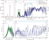 |
Fig. 1 MIRI/MRS (this work), NIRSpec/PRISM, and NIRSpec/G395M Luhman et al. (2024) spectrum of WISE 0855 from 0.8 to 22 µm. Panel a: NIRSpec/PRISM data (in red) from 0.8 to 2.2 m. Panel b: NIRSpec/G395M (in green) and MIRI/MRS data (in blue) from 2.2 to 22 m. Panels c and d: Overlap between the three datasets from 3.5 to 5.4 µm and the ammonia feature from 8.0 to 13.0 µm, respectively. The most dominant absorbing species are presented above the spectrum in various colors. For better visualization he data was binned to a resolution of R = 1000 for MIRI/MRS and NIRSpec/G395M andR= 100 for NIRSpec/PRISM. |
3 Methodology
3.1 Atmospheric retrievals
To understand the atmospheric structure and obtain abundance estimates, we performed a free atmospheric retrieval analysis using the publicly available python package petitRADTRANS (version 2.7.4; Mollière et al. 2019; Nasedkin et al. 2024). We used the sampling algorithm PyMultinest (Buchner et al. 2014) which is based on the nested sampling algorithm MultiNest (Skilling 2004; Feroz & Hobson 2008).
We present the results of three different retrievals. The following parameters are in common for all retrievals: We retrieved for H2O, NH3 , 15NH3, CH4, CO, CO2, H2S, and PH3 gas (assumed to be vertically constant in the atmospheric column), the planet radius, Rp , gravity, log g, and the base temperature, Tbottom , as well as nodes in the temperature structure, where the profile could be adapted. The baseline retrieval assumes a clear atmosphere. We note that we retrieved logarithmic2 mass fractions, but here we report logarithmic volume fractions, which were calculated on the basis of the retrieved values.
To test whether the abundance of water in the gas phase may decrease with altitude even without adding water ice clouds, we performed a second retrieval for a clear atmosphere with a variable water profile with pressure, by adding two free parameters: a pressure level chosen freely throughout the column, pH2O , and an exponent of a power law reducing the initial water mass mixing ratio α. This allows for a decrease or increase at lower pressures compared to the initial water abundance parameterized as shown in Eq. (2):
 (2)
(2)
where M(H2Ocd)(p) denotes the logarithmic mass fraction of water vapor varying with pressure and M(H2Ocd)r the retrieved water vapor value for the lower atmosphere.
Increasing the complexity in the model further, we added clouds in a third retrieval whilst keeping the variable water profile of the second retrieval. We included the water cloud opacities H2Ocd corresponding to spherical ice particles as well as the following cloud parameters: the sedimentation coefficient, fsed , the logarithmic eddy mixing coefficient ,logKzz, the width of the particle size distribution, σlnorm, and the logarithmic pressure at the lower cloud base, logPbase. The amount of cloud particles decreases with height according to a freely retrieved parameter, fsed . Small values of fsed correspond to large extensions of the cloud deck and larger fsed values to smaller cloud extensions. The cloud layer is given by the following parameterization based on the work of Ackerman & Marley (2001) presented in Eq. (3), where M(H2Ocd)(p) corresponds to the logarithmic mass fraction of condensate molecules in the cloud layer varying with pressure, M(H2Ocd)r to the retrieved value of the condensate abundance and pb to the retrieved cloud base layer pressure. In this context, “cd” stands for crystalline and distribution of hollow spheres (DHS) particles approximating a non-spherical shape of crystals (Min et al. 2005). The priors and posteriors of the three retrievals are presented in Table B.1.
 (3)
(3)
To detect the isoptopologue 15NH3 , we performed one additional retrieval: identical to the clear retrieval with constant water profile, but neglecting the opacity of 15NH3 and the associated free parameter for the 15NH3 abundance. In the same manner we tested for 13CO, but could not constrain the molecule. Future work may include the search for more carbon- and nitrogen-based isotopologs.
We used correlated k (c-k) opacities at a wavelength binning of λ/Δλ = 1000. Thus, we binned the MIRI/MRS and NIRSpec/G395M data to the corresponding wavelength grid of petitRADTRANS. The NIRSpec/PRISM dataset, with a resolution of R ~ 100, was retrieved on this resolving power simultaneously with the higher resolution NIRSpec/G395M and MIRI/MRS datasets. The adopted opacities for the retrievals are shown in Fig. B.1.
A forward model simulates 1D emission spectra from a PT profile parameterized depending on an interior temperature and a custom number of nodes, as well as a given set of opacities and their abundances. The PT structure was parameterized using ten nodes, a bottom temperature and a spline interpolation between the nodes as presented in Barrado et al. (2023). Starting from the bottom temperature the nodes defined the factor by which the temperature was changed for the next layer. We chose the nodes in a prior range between 0.2 and 1.0 and the bottom temperature between 100 K and 9000 K. To better constrain the temperature profile, we added a freely retrieved regularization term depending on a penalty parameter, γ (Line et al. 2015). For smaller values of γ, the roughness in the profile is penalized further. This assumption on the one hand leads to smoothed PT profiles that are more consistent with models, but on the other hand this might lead to compensation effects from other parameters for an overly smoothed PT profile. This will be further discussed in Sect. 5.2. The retrievals were run with N = 1000 live points in constant efficiency mode and sampling efficiency of 0.05.
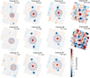 |
Fig. 2 Resulting cube images of channels 1 to 4 with subchannels A to C after dither subtraction. The wavelengths are chosen such that they refer to the detector image with the highest flux at the source in each band. The red circle shows the aperture for the flux extraction of the spectrum at one FWHM of the PSF of the source. The blue circle refers to three times the FWHM on which nine black circles of one FWHM are placed. We extract the flux from each circle and measure the variability to obtain an error that includes the noise in the background, σemp. |
3.2 Self-consistent grid models
To compare the results from the atmospheric retrievals to self- consistently calculated model grids, we fit the data to grid models using the python package species (Stolker et al. 2020) together with the sampling implementation pyMulitnest. The fitted grid models are: ATMO++ (no PH3) (Meisner et al. 2023; Leggett et al. 2021), six models by Lacy and Burrows: cloudy (thick clouds), cloudy (thin clouds) and clear either in chemical equilibrium or disequilibrium (Lacy & Burrows 2023), and the Sonora Elf Owl model (Mukherjee et al. 2024). The grid models can be distinguished in four groups accounting for either cloudy or non-cloudy atmospheres and equilibrium or disequilibrium chemistry and their combinations. We fit one clear and equilibrium chemistry model: Lacy EQ Clear; three clear and non-equilibrium chemistry models: Lacy NEQ Clear, Sonora Elf Owl, ATMO++ (no PH3); two cloudy and equilibrium chemistry models: Lacy EQ cloudy (thick and thin); and two cloudy and disequilibrium chemistry models: Lacy NEQ cloudy (thick and thin). In all subsequent figures, clear and equilibrium chemistry is presented in brown colors, clear and disequilibrium chemistry in reddish colors, cloudy and equilibrium in greenish colors and cloudy and disequilibrium in bluish colors.
The cloudy model by Lacy & Burrows (2023) is available in two different cloud layer thicknesses and they assume a grain size of 10 µm. The thick cloudy Lacy models correspond to the AEE10 grid spectra and the thin cloudy models to the E10 spectra. For the non-equilibrium models the mixing parameter Kzz is set to 106 cm2/s. Using this model grid we fit the effective temperature, the logarithmic gravity and the metallicity.
We compared the data to the Sonora Elf Owl grid Mukherjee et al. (2024). This model probes brown dwarfs of all spectral types ranging down to temperatures of 275 K. The models fit simultaneously for the temperature, gravity, metallicity, and C/O ratio, as well as the eddy diffusion coefficient, Kzz , whereas the latter is assumed to be vertically constant.
We fit the ATMO++ model for the effective temperature and the gravity (Leggett et al. 2021; Meisner et al. 2023). This model removes PH3 as an opacity and includes an adaption to the slope of the PT structure in lower atmospheres as discussed in Tremblin et al. (2015); Leggett et al. (2021) to account for the cooling effect of fingering convection. The strength of the effect is parameterized using the factor γ, which is set to 1.3 in the used model.
For the grid model fits, we used the same binned data as for the retrieval analysis as noted in Sect. 3.1. For the grid model comparisons, we add photometry data from Spitzer, HST, and WISE as they are presented in Table 1 as presented in the “Y dwarf compendium”3.
In addition to the abovementioned parameters, we fitted also for the object’s radius. Using the values for the radius R and the surface gravity g, we calculated the mass using M = 𝑔R2/G, where G is the gravitational constant (Petrus et al. 2024). We obtained luminosity estimates by integrating the flux of the best fit models using the built-in function in the package species.
Photometry used for the self-consistent grid model fits. References correspond to (1) Luhman & Esplin (2016), (2) Schneider et al. (2016), (3) Kirkpatrick et al. (2019), (4) Wright et al. (2014), and (5) Leggett et al. (2017).
4 Results
In the first part, we focus on the water depletion in WISE 0855’s atmosphere. Subsequently, we present the self-consistent models in particular with respect to cloudy compared to clear atmospheres and chemical (dis)equilibrium. Finally, we present the ammonia isotopolog detection and the estimate for the bolometric luminosity.
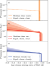 |
Fig. 3 Logarithmic volume mixing ratios varying with pressure for the three shown retrieval results. Panel a: retrieved median clear and constant water profile (solid orange line) and equilibrium chemistry prediction based on the retrieved PT structure (dashed line). Panels b and c: analogs for the clear retrieval with variable water profile (in red), and for the cloudy and variable water profile retrieval (in blue). One to three sigma envelopes are shown around the retrieved profiles. The profiles where parameterized using Eq. (2). |
4.1 Water depletion from atmospheric retrievals
Atmospheric retrievals can infer information about the composition at different pressure levels. In this retrieval setup we vary the water profile using the parameterization presented in Eq. (2) and compare it to the retrieval results from a constant water abundance with height. The pressure level where the retrieval may change the abundance in the atmosphere can be chosen freely. We want to understand whether the retrieval changes the abundance and if so, if the retrieved value can be linked to condensation.
In Fig. 3, we present the fitted volume mixing ratios of water for the three retrievals with cloudy and variable profile in blue, with clear and variable profile in red and with clear and constant water profile in orange. In all cases the shaded areas correspond to one to three sigma variations in the profiles. The chemical equilibrium values are calculated with easyCHEM, an open-source4 Gibbs free energy minimizer to calculate chemical equilibrium compositions presented in Mollière et al. (2017). A Table interpolating easyCHEM results (also including the condensation of water) is available in petitRADTRANS, and we plot the H2O steam abundance for solar metallicity ([Fe/H] = 0) and C/O ratio (C/O = 0.55). The blue dashed line uses the temperature pressure profile from the cloudy retrieval, the red dashed line from the clear retrieval and the orange dashed line from the clear and constant retrieval.
In both the clear and cloudy cases, the bend of the equilibrium profile is inside the three sigma envelope of the fitted profiles and the profiles are compatible with each other. The initial logarithmic water abundance is well constrained and, in the two clear cases, it is comparable with the equilibrium chemistry prediction of −3.18 with logarithmic values of  for the clear and variable profile retrieval and −3.24 ± 0.03 for the clear and constant profile retrieval. We find an initial logarithmic water abundance of −3.07 ± 0.02 for the cloudy retrieval, which is slightly larger compared to the chemical equilibrium expectation. The decrease in abundance of the median profile of the clear retrieval fits the chemical equilibrium expectations well even though the variation is large. The cloudy retrieval decreases less with higher layers compared to the chemical equilibrium prediction. We obtain a pressure where the retrieval changes the water abundance at 10−0.30±0.08 bar for the cloudy retrieval and
  bar for the clear retrieval. The slope for the change in the variable water profile is constrained as
  for the cloudy and
  for the clear case.
Figure 4 shows the pressure-temperature structures of the retrievals in black and gray lines for the cloudy and clear retrievals, respectively. The profiles show the median of 1000 randomly chosen profiles from the posterior distribution with one to three sigmas variation in shaded regions. The retrieved PT structure of the cloudy retrieval is shifted to higher pressures. The dark blue lines correspond to the condensation curves of water for either sub-, super- or solar metallicities ([Fe/H]=- 0.5, 0.5, 0) from Lodders & Fegley (2002). The lines in red and blue show the pressure level freely chosen by the clear and cloudy retrieval respectively, where the water abundance is reduced compared to the initial water abundance. The location of the constrained cloud base by the cloudy retrieval is shown in light blue.
Interestingly, for the clear and the cloudy retrievals the corresponding PT profile crosses the water condensation curve at the height where also the change in water abundance takes place. As the water abundance above the corresponding pressure level decreases (as shown in Fig. 3) and we allow the retrieval to choose the pressure parameter and the reduction in water abundance freely, this provides indication for water condensation in WISE 0855’s atmosphere.
In Fig. 5 we present the resulting spectra from the forward model used in the retrievals with either a constant or variable water profile to present the effect of the water reduction on the spectrum. We used retrieval results from the variable water profiles as inputs to the models either with a constant or with a variable water profile. We see in both the clear and cloudy cases that the spectrum with a variable water profile fits the depth of the water absorption bands better from about 14 µm to 22 µm compared to the one with a constant profile. In addition, we can see a slight improvement of the fit between 6 and 7 µm, corresponding to the water absorption band.
The variable water profile fits significantly better compared to the constant water profile. We find a Bayes factor between the clear and constant water profile retrieval (ln(Z) = 20 468.5) and the clear retrieval with variable water profile (ln(Z) = 20 482.8) of ln(B) = 14.3 corresponding to a 5.7 σ significance. For the cloudy case, between the retrieval with a constant (ln(Z) = 20585.2) and the variable water abundance (ln(Z) = 20616.7) we find a Bayes factor of ln(B) = 31.5 corresponding to a 8.3 σ significance (following the method of Benneke & Seager 2013, to convert ∆lnZ to detection significances).
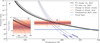 |
Fig. 4 Intersection of the water condensation curve and the retrieved PT profiles compared to the retrieved pressure levels of water depletion. Panel a: median PT profiles for the clear retrieval in gray and the cloudy retrieval in black cross the water condensation curve for sub-, super- and solar metallicities (Lodders & Fegley 2002) shown in dark blue. In a dashed red line we present the freely chosen atmospheric layer, where the water abundances is decreased for the clear retrieval and in blue for the cloudy retrieval. We show one to three sigma envelopes around the median value for the change in water abundance. For both retrievals the crossing between the condensation curve and the PT profile happens at the pressure level chosen freely by the retrieval for the reduction in water abundance indicating that water is likely to condensate out at this height. Panel b: inset to better visualize the crossing area. The light blue line corresponds to the cloud base constrained by the retrieval. |
 |
Fig. 5 Effect of the water depletion on the spectrum. Panel a: comparison of the clear model with the constant water profile (in yellow) and the variable (in red) to the data (in black). Panel b: same but for the cloudy model with the constant profile (in cyan) and variable (in blue). In both panels, we use except for the profile parameters the retrieved values from the variable retrieval as well for the constant model. |
4.2 Clear versus cloudy atmospheric retrievals
Figure 6 shows the best fit models of the cloudy and clear retrievals for a variable H2O profile. Panel a shows the fit of the NIRSpec/PRISM data, where we find a significantly better agreement of the 1.6 µm flux peak for the cloudy model compared to the clear model. Both models underestimate the 1.3 µm flux and the clear model more than the cloudy one. In panel b we present the fit from 2.2 to 22 µm showing the two insets presented in c and d. The residuals become larger beyond 15 µm for both models. In panel c we show the inset to the NIRSpec/G395M wavelength, agreeing well with the data. The residuals are slightly larger between 4.3 and 4.5 µm in the cloudy model compared to the clear model. The methane and ammonia features between 7 to 13 µm are presented in panel d. Between 7 and 12.5 µm, we see a better fit of the cloudy model compared to the clear one of the order of 2 σ in residuals. Here, the clear model underestimates the flux in the peaks and overestimates the flux in the valleys of the absorption lines by about 1.5×10⁻⁴ Jy. The cloudy model fits better and the residuals are smaller while maintaining the residual shape. Between 7 and 8.5 µm the cloudy retrieval models the CH4 band better compared to the clear retrieval, while the clear model shows an offset compared to the data. The abundances found by the retrievals are presented in Table B.1 and their posterior distributions in Fig. B.2.
The cloudy retrieval constrains the cloud parameter, as presented in the corner plot in Fig. B.3. We find a mean cloud particle logarithmic mass fraction of  at the base, a log cloud base pressure at 1.05 ± 0.02, a σlnorm of
  , a logarithmic eddy diffusion factor Kzz of
  , a sedimentation parameter
When comparing the global logarithmic evidence of the two retrievals with variable water abundance using the logarithmic Bayes factor ln(B), we find that the cloudy model (ln(Z) = 20616.7) fits significantly better when compared to the clear fit (ln(Z) = 20482.8) by ln(B) = 133.9, corresponding to 16.6 σ using Benneke & Seager (2013).
The cloudy retrieval constrains the cloud parameter and the Bayes factor offers evidence to support the cloudy model. However, the cloud layer is set deep in the atmosphere at around 10 bars corresponding to temperatures of about ~500 K, where it is not possible to form water ice clouds and where they would not be stable. In addition, the cloud’s particle size is very small, of the order of ~5nm. Exploring whether such small sizes are physical for a water cloud is beyond the scope of this work; however, this may point to the fact that the water cloud can be used to mimic an additional opacity. The dominant effect of the cloud on the spectrum, when comparing with the model produced with a clear and a cloudy atmosphere, can be further reproduced with a gray cloud. Furthermore, potential problems in the cloud parametrization are discussed in Sect. 5.1. Thus, even though the Bayes factor suggests the inclusion of clouds, we did not detect any water ice clouds. However, this cloud might still be real and may thus account for another potentially phosphorous-bearing species condensing out at this depth.
 |
Fig. 6 Best-fit retrieval spectra of the cloudy in blue and the clear retrieval in red. Both models include a variable water profile and are compared to the data in black. Panels a and b: data and retrievals at the wavelength range from 0.8 to 2.2 µm, and at the wavelength from 2.2 µm to 22 µm. Panels c and d: insets from 3.5 to 5.4 µm, and from 7.2 to 13 µm. The latter two panels are included in panel b where their locations are highlighted. In every panel we show the flux in the upper part and the corresponding residual between retrieval and data in the lower plot. For better visibility the presented models and data are re-binned to a resolution of R = 500 for the NIRSpec/G395M and MIRI/MRS and R = 100 for NIRSpec/PRISM wavelengths. |
 |
Fig. 7 Best-fit grid model spectra for the clear ATMO++ in red, the thick cloudy non-equilibrium model by Lacy & Burrows (2023) in blue and the clear non-equilibrium in orange. Panel a: inset of the PRISM data, which has a significant lower amount of flux. Panel b: NIRSpec/G395M and MIRI/MRS dataset. Panels c and d: insets in panel b on the NIRSpec/G395M region and the prominent NH3 absorption feature. The corresponding χ2 values are 2.57, 1.97 and 5.66 for ATMO++, the Lacy cloudy (thick) and clear non-equilibrium model fits. As for the retrievals and for better visibility we re-bined the models and data to a resolution R = 500 for the NIRSpec/G395M and MIRI/MRS and kept NIRSpec/PRISM at R = 100. |
4.3 Clear versus cloudy self-consistent models
To complement the retrieval analysis we fit our data with more physics-informed models such as the radiative-convective equilibrium models by Lacy & Burrows (2023), ATMO++ without PH3 (Leggett et al. 2021; Meisner et al. 2023) and Sonora Elf Owl (Mukherjee et al. 2024). In Fig. 7 we compare the three best-fit results of the clear, the cloudy (thick) models by Lacy & Burrows (2023) and ATMO++. The resulting reduced χ2 values are 5.66, 1.97 and 2.57, respectively. By comparing the best fit models to the data we see the clear model by Lacy & Burrows (2023) shows an overshoot in flux at around 4.3 µm as presented in Fig. 7c) and a constant underestimation in flux between 7.5 and 22 µm. The cloudy model explains the 4.3 µm better compared to the clear ones. The ammonia feature given in Fig. 7d) is best explained by the ATMO++ model, however still underestimating the flux. The ATMO++ model fits well the 1.6 µm peak and the NIRSpec/PRISM wavelengths. A list of reduced χ2 values is presented in Table 2.
4.4 Chemical disequilibrium in retrieved abundances
The composition of the atmosphere at a certain pressure and temperature level gives hints about the dynamics in the atmosphere. From chemical equilibrium calculations we can derive what atmospheric composition we would expect if no mixing were present. If there is a difference in the observed composition compared to the expected one, this indicates that processes leading to non-equilibrium are present.
In Fig. 8, we present the abundances of the trace gases as logarithmic volume mixing ratios resulting from the retrieval analysis for the species: CH4,NH3,CO,CO2, H2S, and PH3. We compare the retrieved values for all retrievals with the chemical equilibrium calculation presented in Mollière et al. (2017).
Here, NH3 shows slightly smaller values than expected from chemical equilibrium and is very well constrained by the retrievals. We find values of −4.22 ± 0.02 for the cloudy retrieval, −4.25 ± 0.04 for the clear and variable water profile retrieval and −4.29 ± 0.03 for the clear and constant water profile retrieval. The equilibrium value is −3.94. We see well constrained values for CO, even though from chemical equilibrium calculations it is not expected to be present. CO has been previously detected by Miles et al. (2020). Here, we find values of −6.74 ± 0.03 for the cloudy retrieval, −6.71 ± 0.04 for the clear and variable water profile retrieval, and −6.85 ± 0.04 for the clear and constant water profile retrieval. This is a strong indication for chemical disequilibrium as in the observed height, CO gets converted to CH4 via chemical reactions.
Here, CH4 is well constrained and shows similar values compared to what is expected from chemical equilibrium predicting a value of −3.34. For the cloudy retrieval, we find −3.12 ± 0.02, for the clear and variable retrieval  and for the clear and constant water profile retrieval −3.37 ± 0.03. For CO2, we retrieved a value of −8.72 ± 0.06 for the cloudy retrieval,
  for the clear and variable water profile, and
  for the clear and constant water profile retrievals. Similarly, as for CO, we would not expect to see CO2 from chemical equilibrium calculations. Thus, this is another hint for disequilibrium chemistry. For PH3 the cross marks the equilibrium chemistry abundance for pressures above 15 bar and the arrow for pressures below 15 bar as PH3 is only expected in the deep atmosphere when in chemical equilibrium. PH3 seems to be constrained in the clear case with constant water profile to
  and clear and variable water profile to −7.95 ± 0.13. However, in the cloudy case we find PH3 to be fairly unconstrained with a value of
  has been detected only to one part per billion in WISE 0855 (Rowland et al. 2024), leading to the conclusion that the larger values in the clear case are compensating for a mismatch in the flux. For H2S we find similar values compared to the chemical equilibrium prediction, even though no clear features of H2 S are visible as seen in the opacity plot (Fig. B.1). For the clear and constant retrieval we estimate
  , for the clear and variable profile
  and for the cloudy retrieval
  . The equilibrium chemistry calculations predict a value of −4.67.
In Fig. C.1, we present the grid model fits for the chemical disequilibrium Sonora Elf Owl model as well as for the Lacy clear and equilibrium model. The Sonora Elf Owl leads to a χ2 value of 6.77 and the clear Lacy equilibrium model to the highest χ2 in this comparison of 12.72. In Fig. C.2 we present the other cloudy models by Lacy & Burrows (2023) for either chemical equilibrium or disequilibrium and two different cloud heights. They result in a χ2 of 2.75, 3.48, 1.97 and 2.48 for the thick and thin cloudy equilibrium chemistry and the thick and thin cloudy disequilibrium chemistry.
 |
Fig. 8 Retrieved logarithmic volume ratios in comparison with chemical equilibrium values for the species: CO, CO2, PH3 , H2S, CH4, NH3 . Black crosses show the expected values for equilibrium chemistry calculated for the cloudy and variable water profile retrieval. Black triangles correspond to equilibrium values smaller than –10. For PH3 we obtain in the lower atmosphere the crossed value and in the upper atmosphere a value lower than the shown x-axis. We depict in blue the retrieved values from the cloudy and variable water profile, in red from the clear and variable water profile and in orange the clear and constant water profile. |
4.5 Grid model comparison
We compare the data of WISE 0855 to the eight different self-consistent grid models previously discussed in Sect. 4.2 and 4.4. We compare the resulting outputs in Fig. C.4 and in Table C.1.
Across the used grid models, the median effective temperature is Teff = 250.4 ± 6.2 K. The cloudy Lacy models consistently result in an effective temperature of 250 K, except for the clear Lacy equilibrium model resulting in a temperature of 261.4 ± 0.6 K and the non-equilibrium cloudy (thin) model in 248.8 ± 0.5 K being the coldest estimate for WISE 0855 stated yet. The clear ATMO++ model result in significantly higher temperatures of 297.4 ± 0.7 K for the one including and neglecting PH3 respectively. The Sonora Elf Owl model also reaches the lower temperature limit, with Teff = 275.0 ± 0.1 K. For the latter we obtain a value for the mixing parameter log(Kzz) = 2.25 ± 0.04 cm2/s and slightly sub-solar C/O ratio of 0.51 ± 0.01. However, as WISE 0855 might be even colder than the lower limit of the temperature range of this grid, it is generally difficult to interpret the results from this model.
The gravity estimates are consistently reaching the lower limit of the grids being log(g) = 3.5 cm/s2 for the Lacy models and 3.23 cm/s2 for the Sonora Elf Owl. They hit the lower boundary of the grid model and thus result in very small errors smaller than 0.001 cm/s2. The ATMO++ model reaches a larger gravity of 4.2 cm/s2. In general, gravities estimated by grid models are smaller compared to the estimate from retrieval analysis, which result in gravities of 4.7 cm/s2 for the clear models and 4.9 cm/s2 for the cloudy model – this is more than ten times larger compared to the self-consistent model estimate. Literature values range from log(g) = 3.5 to 4.5 cm/s2 for a cold brown dwarf like WISE 0855 based on the Sonora Bobcat evolutionary models (Miles et al. 2020). As the grid fits hit often the lower boundary, we fitted the grid models constraining the surface gravity to log(g) = 4.0−5.0 to probe for other global minima when neglecting the lower gravity bound. The resulting grid parameter are presented in Table C.1. Except for ATMO++ and Lacy non-equilibrium clear, the models still go to the lower bound of the surface gravity.
The radius is consistently estimated at around 1 RJ . The Lacy models predict a slightly larger than Jupiter radius of about 1.15−1.40 RJ except for the clear equilibrium model reaching lower radii of 0.94 RJ. ATMO++ reaches the lowest radius of 0.79 RJ and Sonora Elf Owl slightly larger values of 0.98 RJ. The mass can then be calculated from the radius and gravity estimates. For the Lacy models (except for the clear and equilibrium one), we estimate masses of about 2 MJ. Cloudy models predict a higher mass compared to clear models. For the ATMO++ fit we estimate a larger mass of about 3.7 MJ, while Sonora Elf Owl reaches an unrealistically small mass of 0.33 MJ.
The cloudy Lacy models result in subsolar metallicities ranging from [Fe/H] = −0.2 to −0.4. The clear Lacy models and Sonora Elf Owl shows a supersolar metallicites of [Fe/H] = 0.4−0.5. The metallicity of the ATMO++ grid is fixed at solar metallicity.
By integrating the best fit spectra of the self-consistent grid models, we can obtain estimates for the luminosity compared to solar. The values are consistent with a median value of − 7.294 ± 0.023 in logarithmic scale. Cloudy models tend to result in slightly lower values compared to clear models, except of the ATMO++ models reaching similar values compared to the cloudy Lacy models. The values are presented in Table C.2.
The reduced χ2 values for the various models are presented in Table 2. The two smallest reduced χ2 are given by the Lacy non-equilibrium model with thick clouds, followed by the Lacy non-equilibrium model with thin clouds and the ATMO++ model. The largest reduced χ2 results from the Lacy clear and equilibrium model.
Reduced χ2 values for the self-consistent models ordered from the lowest values to the highest.
4.6 Atmospheric structure
The atmospheric structure returned by the retrievals and Lacy grid models is presented by the PT profiles in Fig. 9. We compare the retrieved PT profiles to the profiles of the best-fitting models by Lacy & Burrows (2023) as well as to the PT profile from Jupiter measured by the Galileo probe (Seiff et al. 1998). In addition, we present the contribution function, showing us which atmospheric layer the observed flux per instrument originates from.
In general, the retrieved PT profiles are very similar to each other, however the clear structures seem slightly steeper compared to the cloudy one. Also, the variation in the PT structures are very small especially between 0.3 and 30 bar where we have contributions from the data. All retrieved PT profiles cross the water condensation curve in the area visible by MIRI/MRS as indicated by the contribution functions in gray. In the retrieval we introduced a regularization factor γ which penalizes inversions in the PT structure (Line et al. 2015). This value is well constrained and we obtain values of  for the cloudy,
  for the clear and variable water profile and
  for the clear and constant water profile retrieval. As smaller values correspond to larger constraints on the variability, we penalize the clear profiles more than the cloudy ones. This might lead to the observed steepness difference in the two profiles.
We plot the PT structures of the Lacy NEQ clear and cloudy (thick) models at an effective temperature of 250 K and log(g) = 3.5 at supersolar and subsolar metallicity in orange and blue respectively. In general, the Lacy profiles are slightly steeper in height compared to the retrieval outputs. Shortly after crossing the water condensation curve with height the Lacy models become nearly isothermal along the condensation curve while the retrieved PT profiles are not as steep. The cloudy Lacy PT shows a constant offset compared to the clear one. Higher metallicities shift the PT structure to lower pressures and larger gravities shift the PT structure to higher pressures (Mollière et al. 2015; Fortney 2018). As the Lacy models find lower gravities compared to the retrievals, they will probe the atmosphere at lower pressures. In the lower atmosphere, both Lacy PT profiles provide larger temperatures at a fixed pressure compared to the retrieval profiles.
We show the mean contribution function over the posterior distribution and wavelengths per instrument from the retrievals, showing the height in the atmosphere where the flux per wavelength in the retrieved spectrum originates from. In dark gray we present the contribution of MIRI/MRS, in medium gray of NIR- Spec/G395M and in light gray of NIRSpec/PRISM. At longer wavelengths we are probing colder areas of the atmosphere corresponding to higher altitudes. With MIRI/MRS we are thus probing a region of about 0.3 to 10 bar, with NIRSpec/G395M about 1 to 30 bar and with NIRSpec/PRISM about 3 to 100 bar. The contribution of NIRSpec/G395M shows a strong peak at around 11 bar. This is the pressure level where the clouds are constrained in the cloudy retrieval. However, the clouds seem to be not completely opaque, as the retrieval shows contributions below the cloudy layer with NIRSpec/PRISM down to even 1000 bar. As we do not have many data points in the visible wavelength range, this estimate needs to be taken with caution.
Jupiter’s PT profile is similar to the retrieved profile with a constant offset of about 150 K between about 0.3 and 30 bar, which is also the area where we probe the atmosphere with our data. The upper atmosphere for pressures lower than 0.3 bar the PT profile of Jupiter becomes nearly isothermal. We can see that at about the same height where Jupiter crosses the ammonia condensation curve, WISE 0855 crosses the water condensation curve for the retrieved PT structures and the clear Lacy model.
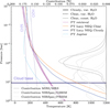 |
Fig. 9 Pressure-temperature (PT) profiles of the retrievals in magenta compared to the H2O and NH3 condensation curves in violet and the contribution functions of MIRI/MRS, NIRSpec/G395M and NIR- Spec/PRISM in gray. Solid lines correspond to the cloudy, variable water profile, dashed lines to the clear and variable water profile and dotted lines to the clear and constant water profile retrievals. We show the mean PT profiles of a 1000 randomly drawn profiles from the posterior distribution. Fainter lines correspond to plus minus one standard deviation from the distribution of profiles. In light blue we present the measured and interpolated PT profiles of Jupiter (Seiff et al. 1998). In blue we compare the pressure temperature profiles at 250K effective temperature of the Lacy NEQ Cloudy (thick) model for subsolar metallicity with the Lacy NEQ Clear model for supersolar metallicity in orange (Lacy & Burrows 2023). At around 10 bars, the height of the constrained cloud based is indicated. The condensation curves for NH3 and H2O are taken from Lodders & Fegley (2002) for solar metallicity. |
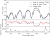 |
Fig. 10 Best-fit spectrum with 15NH3 included in blue, the best fit removing the 15NH3 opacity in red and in black the data with error bars. Panel a: NH3 feature observed by the MIRI/MRS spectrum of WISE 0855. Panel b: residuals of the fit with and without 15NH3 in blue and red respectively. Panel c: 15NH3 opacity used for the retrieval at 277 K and for the pressures of the clear retrieval with varying H2O profile. |
4.7 15NH3 isotopolog abundance
The resolution of MIRI/MRS of up to R ≈ 3750 in the MIR enables us to search for isotopologs. We detect the isotopologue15 NH3 in WISE 0855’s ammonia-rich atmosphere. Comparing the evidence of the atmospheric retrieval with and without15 NH3 (as shown in Table B.2) results in a logarithmic Bayes factor ln(B) = 9.9 favouring the model that includes 15NH3 by 4.8 σ when comparing to Benneke & Seager (2013). In Fig. 10, we present the spectral differences in the models with and without 15NH3 . We found a clear signature of 15NH3 absorption at 9.26, 9.61 µm, 9.97 µm, and 10.11 µm. Here, the residuals of the retrieval without 15NH3 and the opacities offer a very precise match at the same wavelengths, thus enforcing the detection.
From the volume mixing ratios we can calculate the value 14NH3/15NH3 . The distribution of the values is presented in Fig. 11. For the median over a sample of 1000 spectra from the posterior distribution, we obtain a value of  for the cloudy and variable water profile retrieval,
  for the clear and variable water profile retrieval and
  for the clear and constant water profile retrieval. The uncertainty is given by the differences between the median and the 32nd and 68th percentile respectively of the mentioned distribution. The distribution of the values shows a non Gaussian shape with a tail toward larger values. Interestingly, the tail is more pronounced for clear retrievals compared to the cloudy retrieval, which seems to follow more a Gaussian distribution. In Fig. 11 we further compare the ratio to values of the Interstellar Medium (ISM), the Sun, and the first detection in the cold brown dwarf WISE 1828 presented in Barrado et al. (2023).
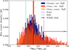 |
Fig. 11 Distribution of the 14NH3/15NH3 ratios for each retrieval with the solid lines marking the corresponding median value. The cyan line represents the value for ISM and the magenta line shows the value for the Sun. The value presented by Barrado et al. (2023) for the brown dwarf WISE 1828 is shown in black and the line indicates the uncertainty. |
4.8 Bolometric luminosity estimate
The broad wavelength range of MIRI/MRS combined with the NIRSpec data provides the possibility to retrieve a bolometric luminosity estimate, as this flux includes the majority of the emergent spectrum of WISE 0855. We integrate the combined spectrum on the original resolution with the empirical and inflated error from 0.8 to 22 µm and add the best fitting ATMO++ model from 22 to 30 µm. We obtain a value of the bolometric luminosity of log(L/L⊙) = −7.291 ± 0.008.
This value is compatible with the previous estimate including the NIRSpec data from Luhman et al. (2024) of log(L/L⊙) = −7.305 ± 0.020. The uncertainty on the luminosity from this work is smaller compared to the value stated in Luhman et al. (2024) as it would be expected by adding more wavelength coverage. For the uncertainty estimate we included the 10b values from the cloudy retrieval.
We can compare the above-stated value to the presented values from the grid model analysis in Table C.2. The median value for the grid models is log(L/L⊙) = −7.294 ± 0.023, which is consistent to the measured estimate by one sigma. The presented values are integrated by a built-in function in species taking the distance and the fitted radius into account. We integrate the model spectra from 0.45 to 30 µm. We do not calculate this value for the Sonora Elf OWL model, as the model spectra are limited up to 15µm.
5 Discussion
5.1 Depletion of water in WISE 0855’s atmosphere
Due to the low effective temperature of WISE 0855 we expect water to condense out. Using the atmospheric retrievals presented in Sect. 4.1 we could detect a lower water abundance in the upper atmosphere of WISE 0855. For both the clear and cloudy case we obtain a Bayes factor which prefers the variable water profile compared to the constant one. Further, when comparing the spectra for constant versus variable water profiles, we see the improvement of the fit at wavelengths larger than 14 µm, shown in Fig. 5. This detection shows the power of MIRI/MRS, as both the long wavelengths as well as the medium resolution are needed to resolve this effect.
We were able to connect the lower water abundance in the upper atmosphere to water condensation by comparing the height of abundance decrease with the water condensation and PT profile intersection. Water condensation, however, does not directly imply cloud formation and indeed our cloud base is constrained too deep in the atmosphere, where temperatures are too large to form water ice.
As particles condensate in the atmosphere they become heavier and might sink down to lower atmospheric layers under the large gravity of brown dwarfs. This would lead to a rainout process similar to what is observed for alkali species in L- and T-type objects (Marley et al. 2002). To be able to form a cloud upward mixing is needed to bring warmer air packets to colder regions leading to condensation of species in the packet. Thus, if we see fast settling of the species this might indicate that vertical mixing is weak and stable water ice clouds would not be possible to observe. However, WISE 0855’s atmosphere shows disequilibrium chemistry which might be explained by rigorous mixing. To understand which effect is the dominant one between upward mixing and settling future variability studies such as the Cycle 1 GO program 2327 may lead to a better understanding of the mixing timescales and thus the dynamics in WISE0855’s atmosphere. Further, the current forward model used in the retrievals might not sufficiently simulate the complex dynamics and interactions with water condensation, cloud formation, rainout processes and many more.
Our retrievals constrain the cloud parameters in the cloudy case, setting a cloud deep into the atmosphere. However, this cloud cannot be a water ice cloud due to the high temperatures at the cloud layer base of up to ∼500 K. There might be multiple reasons for our findings:
Adding a cloud to the retrieval adds an opacity source. Thus, this could mimic a missing opacity in our setup that potentially forms a cloud at higher atmospheric pressures. Interestingly, Morley et al. (2018) showed that a low-lying opacity source might better explain the NIR flux for WISE 0855. They proposed the species NH4H2PO4 as a potential candidate. The condensation curve of NH4H2PO4 in fact intersects at around ∼500 K and 10 bar the modeled PT profile of WISE 0855 as shown in Morley et al. (2018). By comparison, the deep cloud base in the retrieval is set at around 10 bar, which is close to what they found. NH4H2PO4 may be produced from ammonia-, phosphorus- and water-rich lower atmospheres of gas giants (Visscher et al. 2006). Further, Beiler et al. (2024b) propose that a reason for the missing PH3 in cold brown dwarfs might be a condensation of NH4H2PO4 in the lower atmosphere removing PH3 . As we constrain PH3 vaguely in the cloudy retrieval, and clearly constrain PH3 in the clear retrievals, the clouds seem to compensate for adding this species further hinting toward a deep laying opacity source. Thus, we might have revealed a NH4H2PO4 cloud instead of water ice cloud layer in the cloudy retrieval. To test this hypothesis, further investigation on the opacity of this molecule is needed to understand its spectral features.
Instead of an additional opacity source, we can explain the cloud layer as a compensating effect for a steeper PT structure in the lower atmosphere. This was shown by the fact that the ATMO++ model fitted similarly well compared to the cloudy models by Lacy & Burrows (2023). A change in the PT profile in the lower atmosphere induced by fingering convection processes has been proposed by Tremblin et al. (2015). For the retrievals the current setup penalizes changes in the PT structure. Thus, setting a deep opacity might be preferred compared to a change in the PT profile in the lower atmosphere. The clear retrievals result in a larger penalty compared to the cloudy one while showing a steeper PT profile. Thus, the penalty might be the reason for setting rather a cloud layer compared to changing the PT structure enforcing this hypothesis. Further, other PT profile setups may be used, such as a slope fitting parameterization similar to the one presented in Zhang et al. (2023).
Furthermore, the parameterization of the clouds can have an influence on the predicted spectra. Mang et al. (2022) showed that different models for water clouds can lead to significantly different spectra. They compare results from a model including detailed cloud physics with another radiative transfer code based on the parameterization from Ackerman & Marley (2001). They found that they result in incompatible simulated spectra. Thus, the cloud parameterization matters and may strongly vary the resulting spectra. The parameterization used here might be extended in future studies to include more detailed cloud formation processes and structures similarly as presented in Burningham et al. (2021); Vos et al. (2023). In particular the current implementation does not allow for patchy clouds. As discussed in Morley et al. (2014), water clouds often do not form as a homogeneous cloud deck, but rather heterogeneously with clear and cloudy areas. As we average over such an atmosphere, we would expect to see a linear combination of a clear and cloudy atmosphere.
Comparing the self-consistent models to the atmospheric retrievals, we find that either clouds as in the models by Lacy & Burrows (2023) or a PT adaption as in the ATMO++ model is needed to fit the entire spectrum from NIR to MIR. Thus, either one or a combination of the mentioned processes need to be included for fitting WISE 0855’s spectrum.
5.2 PT structure revisited
In our retrieval setup, we do not take any feedback between the PT structure and condensing species into account. The presence of optically thick clouds would lead to heat trapping as it is absorbing radiation in the MIR, preventing the flux that is lower in the atmosphere from escaping. Consequently, this effect would change the PT structure leading to higher temperatures compared to thermodynamic equilibrium around the cloud base (Morley et al. 2012, 2014).
Further, due to the penalty on the PT profile we potentially miss out on such abrupt changes in the PT structure. Thus, other PT parametrizations accounting for such a change coupled to the cloud layer might be useful to test. Rowland et al. (2023) showed that the parameterization might bias the retrieval results and thus more investigations on the effect of the chosen PT structure on the results is needed. Further, cloudy compared to clear preferences in the retrievals might be driven by PT setup choices as presented in Whiteford et al. (2023).
A steeper PT structure in the lower atmosphere was proposed by Tremblin et al. (2015) and could be explained physically by fingering convection. This provides an alternative explanation compared to water ice clouds as we could see in the grid model comparison. Future work on variability measurements might identify patterns only explainable by one of the hypothesis.
The gravity estimated by the self-consistent models is about 14 times lower compared to the estimate of the retrievals. This might explain the large difference between the PT profile of the Lacy & Burrows (2023) models and the retrievals, the latter is shifted by about 10 bars toward higher pressures in the pressure range to which the instrument is sensitive. Also the cloudy retrieval with a larger gravity estimate compared to the two clear ones differ in the PT structure. The cloudy retrieval is shifted toward lower atmospheric layers. As Mollière et al. (2015); Fortney (2018) showed, offsets in the PT profile can be explained by gravity differences. Potentially, these offsets are degenerate with cloud features and/or metallicity estimates.
5.3 Dynamics from chemical disequilibrium
By probing the chemical (dis)equilibrium in brown dwarf atmospheres we can explore the atmospheric dynamics. Fletcher et al. (2020) show how complex it is to model the dynamics in gas giant atmospheres.
As previously stated by Miles et al. (2020), CO is present in the atmosphere of WISE 0855, but would not be abundant in the upper atmosphere in chemical equilibrium as shown in Fig. 8. Thus, this hints toward mixing processes in the atmosphere. The eddy diffusion coefficient quantifies the strength diffusive mixing. Here, our retrieval finds a value of  . This is significantly different from what Miles et al. (2020) found by comparing the M band spectrum to grid models: log(Kzz) = 8.5 cm2 /s corresponding to a much larger diffusion compared to the retrieval estimate. Leggett et al. (2021) confirm the estimate by Miles et al. (2020) by obtaining a value log(Kzz ) = 8.7 cm2/s. From Sonora Elf Owl we get a value of log(Kzz) = 2.25 ± 0.04 cm2/s, which is larger compared to the value from the retrieval, however smaller than the estimates by Miles et al. (2020) and Leggett et al. (2021). Our retrieval estimate however is based on a value derived only from the particle size of the retrieved water cloud and as we do not detect the water ice cloud, this value should be taken with caution. More variability measurements similar to the work presented by Esplin et al. (2016) may offer better constraints on the dynamic processes. Also, by modelling well known objects, such as Jupiter, we might obtain narrower boundary values on priors helping us to improve our constraints on the abundances and bulk parameters, while ruling out certain scenarios.
Based on the findings by Beiler et al. (2024b), CO2 is expected to be more abundant in late T and Y dwarfs than predicted by self-consistent grid models. We find a constraint of CO2 even though the spectral features are not readily visible in neither the 4.2–4.4 µm nor the 15 µm wavelength region. However, retrievals are very sensitive to changes in single molecules and thus a constraint on CO2 is in line with the findings of Beiler et al. (2024b).
From chemical equilibrium we would expect more NH3 compared to N2 in the photosphere (Saumon et al. 2006). However, if we are in a disequilibrium, we would observe a decrease in the NH3 abundance (Leggett et al. 2021; Morley et al. 2018). We detect lower values of NH3 compared to chemical equilibrium estimates. This is a further indication for disequilibrium chemistry. A smaller value of ammonia might also indicate that nitrogen containing species are condensing out in lower layers of the atmospheres. A candidate molecule could be the previously mentioned NH4H2PO4. Depletion of ammonia was identified by Leggett et al. (2015). For methane we find values as they were expected from chemical equilibrium calculations. However, this might not be constant throughout the atmosphere and Morley et al. (2018) see indications for a methane depletion in WISE 0855.
In the presented work, except for water, we use constant abundances of trace molecules, such as CO and CH4 , with height. This is a fair assumption when probing a small wavelength range, as we are then probing only a small part of the atmosphere and as long as the atmosphere is vertically well-mixed. It has been used for many recent retrieval studies (e.g. Barrado et al. 2023; Faherty et al. 2024; Kothari et al. 2024) as the assumption helps to minimize the number of free parameters reducing the runtime as well as the model complexity for the atmospheric retrievals. However, in our case we probe the atmosphere from about 100 to 0.3 bar and we can expect the abundance to vary in this broad height range. Analysis shows how changes in the abundances with height can significantly affect the spectra (Rowland et al. 2023). In future studies, variable profiles for molecules other than water may be included, especially when analyzing broad wavelength ranges now accessible with JWST.
5.4 Evolution of the coldest brown dwarf
Leggett et al. (2021) show their evolutionary models and give estimates for WISE 0855. We can compare our results with their Fig. 11. A temperature of about 300 K and a gravity of log(g) = 4.7 and 4.9 for the clear and cloudy case respectively would lead to ages larger than 10 Gyr, masses of larger than 20 MJ and radii smaller than 1 RJ. In contrast, the estimates from the self-consistent models with a log(g) of 3.5 and a effective temperature of 250 K would result in masses of about 1 MJ , ages of about 0.3 Gyr and radii of about 1.1 RJ . This is compatible with what we find for the Lacy models. When comparing our values to the evolutionary model presented in Marley et al. (2021), we get similar values as presented in Leggett et al. (2021). For the effective temperature of about 250 K and log(g) of 3.5, we obtain a bolometric luminosity of about –7.4, a mass of 1.5 MJ, an age of 0.4 Gyr and a radius of 1.2 RJ. The bolometric luminosity is comparable however slightly smaller compared to our estimate.
Measuring the ratio between 14NH3/15NH3 has been identified as a new formation tracer (Barrado et al. 2023). As discussed in Sect. 4.7 we report a value for the 14NH3/15NH3 ratio of  for the clear retrieval, being closer to the ISM value than the value for the Solar System or WISE 1828 of
  . This means the atmosphere of WISE 0855 seems to be more enriched in 15NH3 compared to the Solar System. Future work might study the implications of this tracer on the age and evolution of WISE 0855. More measurements of isotopologs in brown dwarfs are needed to compare the values, identify trends and to be able to connect to formation conditions and evolutionary models.
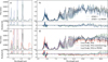 |
Fig. 12 Grid model comparison for ATMO++ (a and b) and Lacy Cloudy non-equilibrium (c and d) if we fit the whole spectrum (green) versus neglecting the NIRSpec/PRISM and photometry data (blue) versus constraining the whole spectrum to log(g) between 4.0 and 5.0 (red). In the case for ATMO++ the grid model results do not change if we only constrain the surface gravity and thus we only show the comparison to the neglected NIRSpec/PRISM data. |
5.5 Challenges in consistently fitting the data
Generally, it is difficult for the self-consistent grid models to fit the entire spectrum across the broad wavelength range. To illustrate this, we show in Fig. 12 the ATMO++ (upper plots) and the cloudy Lacy non-equilibrium fits (lower plots). We present the fits over the entire wavelength range in green and the fit over only NIRSpec/G395M and MIRI/MRS in blue. In both cases, but more prominently in the Lacy fit, the model agrees better with the MIR data if we neglect NIRSpec/PRISM. However, we then obtain an overshoot in the NIR wavelength range. Thus, this indicates that besides a missing opacity source or change in the PT structure even another yet unaccounted effect is needed to explain the full spectrum. The red line shows the cloudy Lacy model with the constrained surface gravity to log(g) = 4.0 to 5.0. In comparison with the unconstrained fit this shows the impact of a higher gravity on the spectrum. However, constraining the gravity does not improve the fit nor does it find another local minimum in which the gravity might be larger as the constrained fit also reaches the lower end of the prior.
How well we fit the data for the grid models per dataset across the wavelength range is presented in Fig. C.3. The cloudy non-equilibrium models by Lacy & Burrows (2023) show the smallest χ2 values for each of the datasets. Comparably well fits the ATMO++ model with similar values as the lowest cloudy grid fit especially in the MIR. Sonora Elf Owl fits the NIR- Spec/PRISM data below 2.2 µm well, but shows larger χ2 for larger wavelengths. Both clear models by Lacy fit significantly worse above 2.2 µm compared to the other models. Note that the overall offsets per dataset are influenced by the retrieved 10b factor added to the error, which varies for each dataset.
Changing the error compared to the pipeline error requires careful consideration as the resulting fit and statistical interpretation depend on this. As discussed in detail in Sect. 2, we inflated the error on the data. The solution presented by Line et al. (2015) by adding an additional offset to the error estimate which is a free parameter of the retrieval works well and has been used in multiple analyses already (e.g. Barrado et al. 2023; Kothari et al. 2024; Rowland et al. 2023). However, we obtain generally very small width in the posterior distributions leading to small uncertainties on the reported values. The resulting width of the posterior distribution might be influenced by the error inflation performed on the fitted dataset. Thus, to better understand where the small errors arise from, further investigations on the impact of the error inflation on the posteriors are needed.
As shown in Rowland et al. (2023) the comparison of free atmospheric retrievals and self-consistent grid models helps set the results of each method into perspective. However, both methods differ in their assumptions and this needs to be taken into account when comparing them. For example we assume constant abundances across the studied pressure range, where self-consistent models vary the abundances. Self-consistent grid models are only able to fit a few parameters, compared to retrievals fitting for several tens of parameters. Thus, the fits of retrievals are often better and may even tend to overfit the data in some instances.
6 Summary and outlook
In this paper, we present the MIR spectrum of WISE 0855 between 5–22 µm observed by JWST MIRI/MRS in combination with an analysis of the MIRI/MRS, NIRSpec/G395M, and NIRSpec/PRISM data (Luhman et al. 2024). We discuss how the mid-infrared adds to existing knowledge of WISE 0855’s atmospheric composition and structure using atmospheric retrievals and self-consistent grid models.
Atmospheric retrievals reveal a depletion of water in the upper atmosphere of WISE 0855 and we could link it to the condensation of water;
We did not detect any clear spectral signatures of water ice particles in the atmosphere of WISE 0855 using either atmospheric retrievals or self-consistent grid models. The cloudy retrieval constrains the cloud parameter, however, the retrieved cloud layer is located too deep in the atmosphere to form stable water ice clouds. This cloud however potentially mimics a phosphorous cloud formed by the proposed species NH4H2PO4;
We would require either a cloud layer or an adaption in the PT profile to be included in the self-consistent grid models to explain the spectrum of WISE 0855;
The cloudy retrieval results in slightly larger equilibrium chemistry values for CH4 , significantly larger values for CO and CO2, slightly smaller values for NH3, and barely constrained values for PH3, in addition to values for H2S that are consistent with chemical equilibrium. Similar values were retrieved in the clear retrievals for all species except for PH3, which were larger than for the cloudy retrieval;
We detected 15NH3 in WISE 0855 and measure its abundance using atmospheric retrievals. The isotopolog ratio is determined as
 for the clear and variable profile retrieval;
We calculated a bolometric luminosity of log(L/L⊙) = −7.291 ± 0.008 by integrating the spectrum and best-fit ATMO++ model from 0.8 to 30 µm.
The MIRI/MRS observation presented in this study enables new possibilities in the atmospheric characterization of WISE 0855 by covering the MIR wavelengths in medium resolution, as shown by the detection of water depletion. The implementation of liquid water in the retrievals could lead to a better understanding of the condensation processes. Deep opacity sources that could potentially be missing might be identified using future retrievals and modeling approaches. Future observations could reveal WISE 0855’s atmospheric variability, potentially identifying patchy clouds and improving the constraints on the atmospheric dynamics and pressure temperature structure. Y dwarfs are fascinating analogues to gas giants both within and beyond our Solar System. MIRI enables their detailed characterization, improving our understanding of the very low temperature regime of brown dwarf atmospheres.
Data availability
The raw data of the MIRI/MRS dataset presented in this paper is available at the Mikulski Archive for Space Telescopes (MAST, https://mast.stsci.edu/portal/Mashup/Clients/Mast/Portal.html) via the Proposal ID: 1230 or directly via this DOI: http://dx.doi.org/10.17909/0tet-zp19 The appendices including Figs. A.1–C.4 and Tables B.1– C.2 are available online on Zenodo via this DOI: https://doi.org/10.5281/zenodo.14762536
Acknowledgements
The authors thank the referee for the constructive feedback improving the quality of this paper. P.-O.L acknowledges funding support by CNES. BV, OA, and PR thank the European Space Agency (ESA) and the Belgian Federal Science Policy Office (BELSPO) for their support in the framework of the PRODEX Programme. NW acknowledges funding from NSF award #2238468, #1909776, and NASA Award #80NSSC22K0142. OA is a Senior Research Associate of the Fonds de la Recherche Scientifique – FNRS. EvD acknowledges support from A-ERC grant 101019751 MOLDISK. DB is supported by Spanish MCIN/AEI/10.13039/501100011033 grant PID2019- 107061GB-C61 and No. MDM-2017-0737. LD acknowledges funding from the KU Leuven Interdisciplinary Grant (IDN/19/028), the European Union H2020- MSCA-ITN-2019 under Grant no. 860470 (CHAMELEON) and the FWO research grant G086217N. MPIA acknowledges support from the Federal Ministry of Economy (BMWi) through the German Space Agency (DLR). PP thanks the Swiss National Science Foundation (SNSF) for financial support under grant number 200020_200399. PT acknowledges support by the European Research Council under Grant Agreement ATMO 757858. JPP acknowledges financial support from the UK Science and Technology Facilities Council, and the UK Space Agency. For the purpose of open access, the author has applied a Creative Commons Attribution (CC BY) licence to the Author Accepted Manuscript version arising from this submission. The Cosmic Dawn Center (DAWN) is funded by the Danish National Research Foundation under grant No. 140. TPR acknowledges support from the ERC through grant no. 743029 EASY. MV is a FRIA grantee of the Fonds de la Recherche Scientifique – FNRS. GO acknowledges support from SNSA.
We refer to the logarithm with base 10 throughout the paper.
References
- Ackerman, A. S., & Marley, M. S. 2001, ApJ, 556 [Google Scholar]
- Adande, G. R., & Ziurys, L. M. 2012, ApJ, 744, 194 [NASA ADS] [CrossRef] [Google Scholar]
- Argyriou, I., Glasse, A., Law, D. R., et al. 2023, A&A, 675 [Google Scholar]
- Barrado, D., Mollière, P., Patapis, P., et al. 2023, Nature, 624, 263 [NASA ADS] [CrossRef] [Google Scholar]
- Beichman, C., Gelino, C. R., Kirkpatrick, J. D., et al. 2014, ApJ, 783 [Google Scholar]
- Beiler, S. A., Cushing, M. C., Kirkpatrick, J. D., et al. 2024a, ApJ, 973, 107 [NASA ADS] [CrossRef] [Google Scholar]
- Beiler, S. A., Mukherjee, S., Cushing, M. C., et al. 2024b, ApJ, 973, 60 [Google Scholar]
- Benneke, B., & Seager, S. 2012, ApJ, 753, 100 [NASA ADS] [CrossRef] [Google Scholar]
- Benneke, B., & Seager, S. 2013, ApJ, 778, 153 [Google Scholar]
- Böker, T., Beck, T. L., Birkmann, S. M., et al. 2023, PASP, 135, 038001 [CrossRef] [Google Scholar]
- Buchner, J., Georgakakis, A., Nandra, K., et al. 2014, A&A, 564 [Google Scholar]
- Burningham, B., Faherty, J. K., Gonzales, E. C., et al. 2021, MNRAS, 506, 1944 [NASA ADS] [CrossRef] [Google Scholar]
- Burrows, A., Marley, M., Hubbard, W. B., et al. 1997, ApJ, 491, 856 [Google Scholar]
- Burrows, A., Sudarsky, D., & Lunine, J. I. 2003, ApJ, 596, 587 [CrossRef] [Google Scholar]
- Bushouse, H., Eisenhamer, J., Dencheva, N., et al. 2023, https://doi.org/10.5281/zenodo.7577320 [Google Scholar]
- Coulter, D. J., Barnes, J. W., & Fortney, J. J. 2022, ApJS, 263, 15 [NASA ADS] [Google Scholar]
- Cushing, M. C., Kirkpatrick, J. D., Gelino, C. R., et al. 2011, ApJ, 743 [Google Scholar]
- Esplin, T. L., Luhman, K. L., Cushing, M. C., et al. 2016, ApJ, 832, 58 [NASA ADS] [CrossRef] [Google Scholar]
- Faherty, J. K., Tinney, C. G., Skemer, A., & Monson, A. J. 2014, ApJ, 793 [Google Scholar]
- Faherty, J. K., Burningham, B., Gagné, J., et al. 2024, Nature, 628, 511 [NASA ADS] [CrossRef] [Google Scholar]
- Feroz, F., & Hobson, M. P. 2008, MNRAS, 384, 449 [NASA ADS] [CrossRef] [Google Scholar]
- Fletcher, L. N., Kaspi, Y., Guillot, T., & Showman, A. P. 2020, Space Sci. Rev., 216, 30 [NASA ADS] [CrossRef] [Google Scholar]
- Fortney, J. J. 2018, arXiv e-prints [arXiv:1804.08149] [Google Scholar]
- Gardner, J. P., Mather, J. C., Abbott, R., et al. 2023, PASP, 135, 068001 [NASA ADS] [CrossRef] [Google Scholar]
- Jones, O. C., Álvarez Márquez, J., Sloan, G. C., et al. 2023, MNRAS, 523, 2519 [Google Scholar]
- Kirkpatrick, J. D., Martin, E. C., Smart, R. L., et al. 2019, ApJS, 240, 19 [NASA ADS] [CrossRef] [Google Scholar]
- Kothari, H., Cushing, M. C., Burningham, B., et al. 2024, ApJ, 971, 121 [NASA ADS] [CrossRef] [Google Scholar]
- Lacy, B., & Burrows, A. 2023, ApJ, 950, 8 [NASA ADS] [CrossRef] [Google Scholar]
- Law, D. R. E., Morrison, J., Argyriou, I., et al. 2023, ApJ, 166, 45 [Google Scholar]
- Leggett, S. K., Morley, C. V., Marley, M. S., & Saumon, D. 2015, ApJ, 799, 37 [NASA ADS] [CrossRef] [Google Scholar]
- Leggett, S. K., Tremblin, P., Esplin, T. L., Luhman, K. L., & Morley, C. V. 2017, ApJ, 842, 118 [NASA ADS] [CrossRef] [Google Scholar]
- Leggett, S. K., Tremblin, P., Phillips, M. W., et al. 2021, ApJ, 918, 11 [NASA ADS] [CrossRef] [Google Scholar]
- Line, M. R., Teske, J., Burningham, B., Fortney, J. J., & Marley, M. S. 2015, ApJ, 807, 183 [NASA ADS] [CrossRef] [Google Scholar]
- Lodders, K., & Fegley, B. 2002, Icarus, 155, 393 [Google Scholar]
- Luhman, K. L. 2014, ApJ, 786, L18 [Google Scholar]
- Luhman, K. L., & Esplin, T. L. 2016, AJ, 152, 78 [NASA ADS] [CrossRef] [Google Scholar]
- Luhman, K. L., Tremblin, P., de Oliveira, C. A., et al. 2024, ApJ, 167, 5 [Google Scholar]
- Madhusudhan, N., & Seager, S. 2009, ApJ, 707, 24 [NASA ADS] [CrossRef] [Google Scholar]
- Mahaffy, P. R., Niemann, H. B., Alpert, A., et al. 2000, J. Geophys. Res., 105, 15061 [Google Scholar]
- Mang, J., Gao, P., Hood, C. E., et al. 2022, ApJ, 927, 184 [NASA ADS] [CrossRef] [Google Scholar]
- Marley, M. S., Seager, S., Saumon, D., et al. 2002, ApJ, 568, 335 [NASA ADS] [CrossRef] [Google Scholar]
- Marley, M. S., Saumon, D., Visscher, C., et al. 2021, ApJ, 920, 85 [NASA ADS] [CrossRef] [Google Scholar]
- Matthews, E. C., Carter, A. L., Pathak, P., et al. 2024, Nature, 633, 789 [NASA ADS] [CrossRef] [Google Scholar]
- Mawet, D., Milli, J., Wahhaj, Z., et al. 2014, ApJ, 792, 11 [CrossRef] [Google Scholar]
- Meisner, A. M., Leggett, S. K., Logsdon, S. E., et al. 2023, AJ, 166, 57 [NASA ADS] [CrossRef] [Google Scholar]
- Miles, B. E., Skemer, A. J. I., Morley, C. V., et al. 2020, AJ, 160, 63 [NASA ADS] [CrossRef] [Google Scholar]
- Min, M., Hovenier, J., Dekoter, A., Waters, L., & Dominik, C. 2005, Icarus, 179, 158 [Google Scholar]
- Mollière, P., Boekel, R. V., Dullemond, C., Henning, T., & Mordasini, C. 2015, ApJ, 813, 47 [CrossRef] [Google Scholar]
- Mollière, P., van Boekel, R., Bouwman, J., et al. 2017, A&A, 600, A10 [Google Scholar]
- Mollière, P., Wardenier, J. P., van Boekel, R., et al. 2019, A&A, 627, A67 [Google Scholar]
- Mollière, P., Stolker, T., Lacour, S., et al. 2020, A&A, 640, A131 [Google Scholar]
- Morley, C. V., Fortney, J. J., Marley, M. S., et al. 2012, ApJ, 756, 172 [NASA ADS] [CrossRef] [Google Scholar]
- Morley, C. V., Marley, M. S., Fortney, J. J., et al. 2014, ApJ, 787, 78 [Google Scholar]
- Morley, C. V., Skemer, A. J., Allers, K. N., et al. 2018, ApJ, 858, 97 [Google Scholar]
- Mukherjee, S., Fortney, J. J., Morley, C. V., et al. 2024, ApJ, 963, 73 [NASA ADS] [CrossRef] [Google Scholar]
- Nasedkin, E., Mollière, P., & Blain, D. 2024, J. Open Source Softw., 9, 5875 [CrossRef] [Google Scholar]
- Nomura, H., Furuya, K., Cordiner, M. A., et al. 2022, arXiv e-prints [arXiv:2203.10863] [Google Scholar]
- Petrus, S., Whiteford, N., Patapis, P., et al. 2024, ApJ, 966, L11 [NASA ADS] [CrossRef] [Google Scholar]
- Phillips, M. W., Tremblin, P., Baraffe, I., et al. 2020, A&A, 637, A38 [NASA ADS] [CrossRef] [EDP Sciences] [Google Scholar]
- Rigby, J., Perrin, M., McElwain, M., et al. 2023, PASP, 135, 048001 [NASA ADS] [CrossRef] [Google Scholar]
- Rowland, M. J., Morley, C. V., & Line, M. R. 2023, ApJ, 947, 6 [NASA ADS] [CrossRef] [Google Scholar]
- Rowland, M. J., Morley, C. V., Miles, B. E., et al. 2024, ApJ, 977, L49 [Google Scholar]
- Saumon, D., Geballe, T. R., Leggett, S. K., et al. 2000, ApJ, 541, 374 [NASA ADS] [CrossRef] [Google Scholar]
- Saumon, D., Marley, M. S., Cushing, M. C., et al. 2006, ApJ, 647, 552 [NASA ADS] [Google Scholar]
- Saumon, D., Marley, M. S., Abel, M., Frommhold, L., & Freedman, R. S. 2012, ApJ, 750, 74 [Google Scholar]
- Schneider, A. C., Cushing, M. C., Kirkpatrick, J. D., & Gelino, C. R. 2016, ApJ, 823, L35 [Google Scholar]
- Seiff, A., Kirk, D. B., Knight, T. C., et al. 1998, J. Geophys. Res. Planets, 103, 22857 [CrossRef] [Google Scholar]
- Skemer, A. J., Morley, C. V., Allers, K. N., et al. 2016, ApJ, 826, L17 [Google Scholar]
- Skilling, J. 2004, in AIP, 735, 395 [NASA ADS] [Google Scholar]
- Stolker, T., Quanz, S. P., Todorov, K. O., et al. 2020, A&A, 635, A182 [EDP Sciences] [Google Scholar]
- Tremblin, P., Amundsen, D. S., Mourier, P., et al. 2015, ApJ, 804, L17 [CrossRef] [Google Scholar]
- Tremblin, P., Padioleau, T., Phillips, M. W., et al. 2019, ApJ, 876, 144 [Google Scholar]
- Visscher, C., Lodders, K., & Fegley, B., Jr. 2006, ApJ, 648, 1181 [NASA ADS] [CrossRef] [Google Scholar]
- Vos, J. M., Burningham, B., Faherty, J. K., et al. 2023, ApJ, 944, 138 [NASA ADS] [CrossRef] [Google Scholar]
- Wells, M., Pel, J.-W., Glasse, A., et al. 2015, PASP, 127, 646–664 [NASA ADS] [CrossRef] [Google Scholar]
- Whiteford, N., Glasse, A., Chubb, K. L., et al. 2023, MNRAS, 525, 1375 [NASA ADS] [CrossRef] [Google Scholar]
- Wright, E. L., Mainzer, A., Davy Kirkpatrick, J., et al. 2014, ApJ, 148, 82 [Google Scholar]
- Wright, G. S., Wright, D., Goodson, G. B., et al. 2015, PASP, 127, 595 [NASA ADS] [CrossRef] [Google Scholar]
- Wright, G. S., Rieke, G. H., Glasse, A., et al. 2023, PASP, 135, 048003 [NASA ADS] [CrossRef] [Google Scholar]
- Zahnle, K. J., & Marley, M. S. 2014, ApJ, 797, 19 [NASA ADS] [CrossRef] [Google Scholar]
- Zhang, Y., Snellen, I. A. G., Bohn, A. J., et al. 2021, Nature, 595, 370 [NASA ADS] [CrossRef] [Google Scholar]
- Zhang, Z., Mollière, P., Hawkins, K., et al. 2023, AJ, 166, 198 [NASA ADS] [CrossRef] [Google Scholar]
All Tables
Photometry used for the self-consistent grid model fits. References correspond to (1) Luhman & Esplin (2016), (2) Schneider et al. (2016), (3) Kirkpatrick et al. (2019), (4) Wright et al. (2014), and (5) Leggett et al. (2017).
Reduced χ2 values for the self-consistent models ordered from the lowest values to the highest.
All Figures
|
Fig. 1 MIRI/MRS (this work), NIRSpec/PRISM, and NIRSpec/G395M Luhman et al. (2024) spectrum of WISE 0855 from 0.8 to 22 µm. Panel a: NIRSpec/PRISM data (in red) from 0.8 to 2.2 m. Panel b: NIRSpec/G395M (in green) and MIRI/MRS data (in blue) from 2.2 to 22 m. Panels c and d: Overlap between the three datasets from 3.5 to 5.4 µm and the ammonia feature from 8.0 to 13.0 µm, respectively. The most dominant absorbing species are presented above the spectrum in various colors. For better visualization he data was binned to a resolution of R = 1000 for MIRI/MRS and NIRSpec/G395M andR= 100 for NIRSpec/PRISM. |
| In the text | |
|
Fig. 2 Resulting cube images of channels 1 to 4 with subchannels A to C after dither subtraction. The wavelengths are chosen such that they refer to the detector image with the highest flux at the source in each band. The red circle shows the aperture for the flux extraction of the spectrum at one FWHM of the PSF of the source. The blue circle refers to three times the FWHM on which nine black circles of one FWHM are placed. We extract the flux from each circle and measure the variability to obtain an error that includes the noise in the background, σemp. |
| In the text | |
|
Fig. 3 Logarithmic volume mixing ratios varying with pressure for the three shown retrieval results. Panel a: retrieved median clear and constant water profile (solid orange line) and equilibrium chemistry prediction based on the retrieved PT structure (dashed line). Panels b and c: analogs for the clear retrieval with variable water profile (in red), and for the cloudy and variable water profile retrieval (in blue). One to three sigma envelopes are shown around the retrieved profiles. The profiles where parameterized using Eq. (2). |
| In the text | |
|
Fig. 4 Intersection of the water condensation curve and the retrieved PT profiles compared to the retrieved pressure levels of water depletion. Panel a: median PT profiles for the clear retrieval in gray and the cloudy retrieval in black cross the water condensation curve for sub-, super- and solar metallicities (Lodders & Fegley 2002) shown in dark blue. In a dashed red line we present the freely chosen atmospheric layer, where the water abundances is decreased for the clear retrieval and in blue for the cloudy retrieval. We show one to three sigma envelopes around the median value for the change in water abundance. For both retrievals the crossing between the condensation curve and the PT profile happens at the pressure level chosen freely by the retrieval for the reduction in water abundance indicating that water is likely to condensate out at this height. Panel b: inset to better visualize the crossing area. The light blue line corresponds to the cloud base constrained by the retrieval. |
| In the text | |
|
Fig. 5 Effect of the water depletion on the spectrum. Panel a: comparison of the clear model with the constant water profile (in yellow) and the variable (in red) to the data (in black). Panel b: same but for the cloudy model with the constant profile (in cyan) and variable (in blue). In both panels, we use except for the profile parameters the retrieved values from the variable retrieval as well for the constant model. |
| In the text | |
|
Fig. 6 Best-fit retrieval spectra of the cloudy in blue and the clear retrieval in red. Both models include a variable water profile and are compared to the data in black. Panels a and b: data and retrievals at the wavelength range from 0.8 to 2.2 µm, and at the wavelength from 2.2 µm to 22 µm. Panels c and d: insets from 3.5 to 5.4 µm, and from 7.2 to 13 µm. The latter two panels are included in panel b where their locations are highlighted. In every panel we show the flux in the upper part and the corresponding residual between retrieval and data in the lower plot. For better visibility the presented models and data are re-binned to a resolution of R = 500 for the NIRSpec/G395M and MIRI/MRS and R = 100 for NIRSpec/PRISM wavelengths. |
| In the text | |
|
Fig. 7 Best-fit grid model spectra for the clear ATMO++ in red, the thick cloudy non-equilibrium model by Lacy & Burrows (2023) in blue and the clear non-equilibrium in orange. Panel a: inset of the PRISM data, which has a significant lower amount of flux. Panel b: NIRSpec/G395M and MIRI/MRS dataset. Panels c and d: insets in panel b on the NIRSpec/G395M region and the prominent NH3 absorption feature. The corresponding χ2 values are 2.57, 1.97 and 5.66 for ATMO++, the Lacy cloudy (thick) and clear non-equilibrium model fits. As for the retrievals and for better visibility we re-bined the models and data to a resolution R = 500 for the NIRSpec/G395M and MIRI/MRS and kept NIRSpec/PRISM at R = 100. |
| In the text | |
|
Fig. 8 Retrieved logarithmic volume ratios in comparison with chemical equilibrium values for the species: CO, CO2, PH3 , H2S, CH4, NH3 . Black crosses show the expected values for equilibrium chemistry calculated for the cloudy and variable water profile retrieval. Black triangles correspond to equilibrium values smaller than –10. For PH3 we obtain in the lower atmosphere the crossed value and in the upper atmosphere a value lower than the shown x-axis. We depict in blue the retrieved values from the cloudy and variable water profile, in red from the clear and variable water profile and in orange the clear and constant water profile. |
| In the text | |
|
Fig. 9 Pressure-temperature (PT) profiles of the retrievals in magenta compared to the H2O and NH3 condensation curves in violet and the contribution functions of MIRI/MRS, NIRSpec/G395M and NIR- Spec/PRISM in gray. Solid lines correspond to the cloudy, variable water profile, dashed lines to the clear and variable water profile and dotted lines to the clear and constant water profile retrievals. We show the mean PT profiles of a 1000 randomly drawn profiles from the posterior distribution. Fainter lines correspond to plus minus one standard deviation from the distribution of profiles. In light blue we present the measured and interpolated PT profiles of Jupiter (Seiff et al. 1998). In blue we compare the pressure temperature profiles at 250K effective temperature of the Lacy NEQ Cloudy (thick) model for subsolar metallicity with the Lacy NEQ Clear model for supersolar metallicity in orange (Lacy & Burrows 2023). At around 10 bars, the height of the constrained cloud based is indicated. The condensation curves for NH3 and H2O are taken from Lodders & Fegley (2002) for solar metallicity. |
| In the text | |
|
Fig. 10 Best-fit spectrum with 15NH3 included in blue, the best fit removing the 15NH3 opacity in red and in black the data with error bars. Panel a: NH3 feature observed by the MIRI/MRS spectrum of WISE 0855. Panel b: residuals of the fit with and without 15NH3 in blue and red respectively. Panel c: 15NH3 opacity used for the retrieval at 277 K and for the pressures of the clear retrieval with varying H2O profile. |
| In the text | |
|
Fig. 11 Distribution of the 14NH3/15NH3 ratios for each retrieval with the solid lines marking the corresponding median value. The cyan line represents the value for ISM and the magenta line shows the value for the Sun. The value presented by Barrado et al. (2023) for the brown dwarf WISE 1828 is shown in black and the line indicates the uncertainty. |
| In the text | |
|
Fig. 12 Grid model comparison for ATMO++ (a and b) and Lacy Cloudy non-equilibrium (c and d) if we fit the whole spectrum (green) versus neglecting the NIRSpec/PRISM and photometry data (blue) versus constraining the whole spectrum to log(g) between 4.0 and 5.0 (red). In the case for ATMO++ the grid model results do not change if we only constrain the surface gravity and thus we only show the comparison to the neglected NIRSpec/PRISM data. |
| In the text | |
Current usage metrics show cumulative count of Article Views (full-text article views including HTML views, PDF and ePub downloads, according to the available data) and Abstracts Views on Vision4Press platform.
Data correspond to usage on the plateform after 2015. The current usage metrics is available 48-96 hours after online publication and is updated daily on week days.
Initial download of the metrics may take a while.