| Issue |
A&A
Volume 699, July 2025
|
|
|---|---|---|
| Article Number | A219 | |
| Number of page(s) | 27 | |
| Section | Planets, planetary systems, and small bodies | |
| DOI | https://doi.org/10.1051/0004-6361/202453186 | |
| Published online | 14 July 2025 | |
Cloud and haze parameterization in atmospheric retrievals: Insights from Titan's Cassini data and JWST observations of hot Jupiters
1
Kapteyn Institute, University of Groningen,
9747
AD Groningen,
The Netherlands
2
Department of Physics and Astronomy, University College London,
WC1E 6BT
London,
UK
3
Université Paris Cité and Univ Paris Est Creteil, CNRS, LISA,
75013
Paris,
France
4
University of Bristol, School of Physics, HH Wills Physics Laboratory,
Tyndall Avenue,
Bristol
BS8 1TL,
UK
5
Universite Paris Cite, Universite Paris-Saclay, CEA, CNRS, AIM,
91191
Gif-sur-Yvette,
France
6
Space Telescope Science Institute,
3700 San Martin Drive,
Baltimore,
MD
21218,
USA
7
SRON, Netherlands Institute for Space Research,
Niels Bohrweg 4,
2333
CA Leiden,
The Netherlands
8
Division of Science, National Astronomical Observatory of Japan,
2-21-1 Osawa, Mitaka-shi,
Tokyo,
Japan
★ Corresponding author: This email address is being protected from spambots. You need JavaScript enabled to view it.
Received:
26
November
2024
Accepted:
19
May
2025
Abstract
Context. Before JWST, telescope observations were not sensitive enough to constrain the nature of clouds in exo-atmospheres. Recent observations, however, have inferred cloud signatures as well as haze-enhanced scattering slopes motivating the need for modern inversion techniques and a deeper understanding of the JWST information content.
Aims. We aim to investigate the information content of JWST exoplanet spectra. We particularly focus on designing an inversion technique able to handle a wide range of cloud and hazes.
Methods. We built a flexible aerosol parameterization within the TAUREX framework, enabling us to conduct atmospheric retrievals of planetary atmospheres. The method is evaluated on available Cassini occultations of Titan. We then use the model to interpret the recent JWST data for the prototypical hot Jupiters HAT-P-18 b, WASP-39 b, WASP-96 b, and WASP-107 b. In parallel, we performed complementary simulations on controlled scenarios to further understand the information content of JWST data and provide parameterization guidelines.
Results. Our results use free and kinetic chemistry retrievals to extract the main atmospheric properties of key JWST exoplanets, including their main molecular abundances (and elemental ratios), thermal structures, and aerosol properties. In our investigations, we show the need for a wide wavelength coverage to robustly characterize clouds and hazes - which is necessary to mitigate biases arising from our lack of priors on their composition - and break degeneracies with atmospheric chemical composition. With JWST, the characterization of clouds and hazes might be difficult, due to the lack of simultaneous wavelength coverage from visible to mid-infrared by a single instrument and the likely presence of temporal variability between visits (from e.g., observing conditions, instrument systematics, stellar host variability, or planetary weather).
Key words: techniques: spectroscopic / planets and satellites: atmospheres / infrared: planetary systems
© The Authors 2025
 Open Access article, published by EDP Sciences, under the terms of the Creative Commons Attribution License (https://creativecommons.org/licenses/by/4.0), which permits unrestricted use, distribution, and reproduction in any medium, provided the original work is properly cited.
This article is published in open access under the Subscribe to Open model. This email address is being protected from spambots. You need JavaScript enabled to view it. to support open access publication.
1 Introduction
Population surveys by the Hubble Space Telescope (HST) have long revealed the ubiquitous presence of aerosols (i.e., suspended solid or liquid particles, including clouds and hazes) in exoplanet atmospheres (Sing et al. 2016; Tsiaras et al. 2018; Min et al. 2020; Estrela et al. 2022; Edwards et al. 2023; Fairman et al. 2024), importantly affecting their chemical and energy balance. Recently, observations have provided clues about their composition (Miles et al. 2023; Dyrek et al. 2024; Grant et al. 2023; Voyer et al. 2025), their complex spatial distribution (Miles et al. 2023), and their time variability (Changeat et al. 2024). With the increase in data quality offered by the recently launched James Webb Space Telescope (JWST), atmospheric retrievals - the statistical inversion technique used to extract the information from spectroscopic exoplanet data - need to incorporate complex representations of clouds and hazes. Simplified assumptions from the HST-era (e.g., homogeneous gray clouds or heuristic power laws) are no longer expected to hold with JWST and should be challenged in the context of those novel observations. Given the expected diversity of aerosol signatures (Gao et al. 2021) and the various observing options provided by JWST, it is difficult to know a priori the level of sophistication required to interpret a given dataset. In this work, we use a flexible parameterization for clouds and hazes incorporated in the TAUREX retrieval framework (Al-Refaie et al. 2021, 2022) to conduct such an exploration. The overarching goal of this paper is twofold: 1) to present a flexible parameterization for aerosols compatible with the TAUREX suite and 2) to explore retrievable aerosol properties from JWST observations. Our software and methodology are described in Section 2. In Section 3, we evaluate our retrieval strategy on the Solar-system moon Titan, as observed by the Cassini spacecraft. Section 4 explores a few JWST cases with the JWST/NIRISS instrument (i.e., HAT-P-18 b, WASP-39 b, and WASP-96 b), and provides a comprehensive analysis of the full WASP-107 b dataset (HST/WFC3, JWST/NIRSpec, JWST/NIRCam, and JWST/MIRI data), focusing on the characterization of aerosols. Lastly, in Section 5, we discuss the more general implications of our experiments for the retrievals of clouds and hazes in the JWST era and provide complementary simulated cases.
2 Methodology
We employed the TAUREX3 retrieval framework (Al-Refaie et al. 2021). TAUREX3 relies on a modern code design with a convenient plugin system for rapid prototyping of new functions (Al-Refaie et al. 2022). To conduct our exploration, we utilized the plugin feature to introduce three open-source plugins: TAUREX-PYMIESCATT1, TAUREX-MULTIMODEL2, and TAUREX-INSTRUMENTSYSTEMATICS3. Central to this paper, TAUREX-PYMIESCATT provides flexible modeling and retrieval of parameterized aerosols using the open-source python library PYMIESCATT (Sumlin et al. 2018) and the phenomenological cloud model from Lee et al. (2013), hereby L13. This is described in more detail in the Appendix. The TAUREX-MULTIMODEL allows us to simulate inhomogeneous atmospheres by combining multiple TAUREX forward models - with independent or coupled parameters - and by weighting their contribution to produce the final observed signal (i.e., eclipse flux ratio or transit depth). TAUREX-INSTRUMENTSYSTEMATICS allows us to treat instrumental systematics when combining observations from different instruments and/or epochs (see also Yip et al. 2021).
In TAUREX-PYMIESCATT, cloud and haze layers are defined by their extinction coefficient (Qext), the particle size distribution (i.e., modeled as a log-normal, a modified gamma, or a one-parameter gamma distribution), the mean pressure of the layer (P) and its range (ΔP), and the particle number density (χ). Multiple particle size distributions are available but for this work we primarily employ the one-parameter gamma distribution introduced in Budaj et al. (2015), which is uniquely defined by the critical radius of the aerosol particles (μr). TAUREX-PYMIESCATT can also model porous particles and aggregates, but in this work, we concentrate on spherical particles since such a level of characterization is difficult with JWST spectra (see Section 5). Additionally, recent studies have highlighted the likely presence and signature of spatially scattered (or partial) clouds, which could be induced by atmospheric circulation. Partial cloud coverage can be modeled by combining a clear and a cloudy forward model with the TAUREX-MULTIMODEL plugin. To illustrate the developments made in this work, we show forward model spectra for various possible cloud scenarios in Figure A1, inspired by the recent results of the prototypical hot Jupiter WASP-107 b (Dyrek et al. 2024; Welbanks et al. 2024; Sing et al. 2024). Relevant literature for the opacity sources we used in this work is available in Table 1 with the data being available online. TAUREX and its plugins are used to perform atmospheric retrievals of Cassini and JWST data for which the setups are briefly described below.
Cassini retrievals. From 2006 to 2011, the Cassini spacecraft obtained 10 occultations of Titan using the Visual and Infrared Mapping Spectrometer (VIMS), four of which are consolidated in Robinson et al. (2014). The other six could not be recovered due to technical issues. The transit-like spectra in Robinson et al. (2014) cover the wavelengths λ ∈ [0.88,5] μm and are ideal to benchmark exoplanet models because of our extensive knowledge of Titan’s atmosphere and in situ measurements. However, our exploration of this Titan data does not aim to replicate the breadth of knowledge accumulated over half a century of observations of this atmosphere. Instead, we seek to illustrate the retrievable atmospheric properties that could be deduced should a similar exoplanet atmosphere be observed. We performed TAUREX retrievals on the data of Robinson et al. (2014) focusing on the recovery of the chemistry and aerosol properties. The retrievals included Rayleigh Scattering, Collision Induced Absorption (CIA for N2-N2, N2-CH4, and CH4-CH4), molecular absorption (CH4, CO, C2H2, C2H4, C2H6, and C2H8), and aerosols. Here, we considered tholin hazes, and condensate CH4(l) clouds. Hazes are thought to produce the blue-ward scattering slope seen in the Titan data, as well as contributing to enhanced absorption around λ = 3.4 μm (Bellucci et al. 2009; Cours et al. 2020) from C-H stretching. We combined the most recent optical data from Rannou et al. (2010) with those from Khare et al. (1984) to construct an updated, broad wavelength (λ ∈ [0.4,5.5] μm), set of refractive indexes for tholins (see Table B.1). We perform two sets of retrievals: 1) retrievals with the exoplanet optimized cross-sections from the ExoMol project (Tennyson et al. 2016; Chubb et al. 2021; Tennyson et al. 2024), and 2) retrievals with HITRAN generated cross-sections4 using the HAPI tool (Kochanov et al. 2016). For each set of crosssections, we tested a haze-only case and a haze+CH4(l) case, using independent aerosol layers of constant particle number density (this hypothesis is discussed more in Section 5). Here, the CH4(l) condensate cloud layer acts as a simple proxy for the complex methane/ethane aerosol cycle happening in the troposphere of Titan. However, we note that this is not intended to fully model the region. In the retrievals presented in the main text, the atmosphere is mainly composed of N2 and CH4, with XCH4 = 0.01485 (Niemann et al. 2010), and we fixed the thermal profile to the one presented in Fulchignoni et al. (2005). In Figure B.2 of the appendix, we remove these two assumptions (i.e., we retrieve the thermal profile and abundance of CH4), highlighting retrieval degeneracies commonly faced in exoplanet transit studies (Rocchetto et al. 2016; Changeat et al. 2020b; Di Maio et al. 2023; Schleich et al. 2024). We retrieve the abundances of trace molecules using log Gaussian priors (μS from Coustenis et al. 2016, σs = 0.5) and the cloud parameters using uninformative uniform priors.
JWST retrievals. Recently JWST has obtained exoplanet spectra of similar signal-to-noise and resolution to the Cassini occultation data. We here explore the information contained at short wavelength using transit observations of HAT-P-18 b, WASP-39 b, and WASP-96 b by the Near Infrared Imager and Slitless Spectrograph (NIRISS). We then perform a more complete exploration of WASP-107 b, which has been extensively observed. WASP-107 b has observations at short wavelengths -from the Hubble Wide Field Camera 3 G102 and G141 Grisms - and recent data from the Near Infrared Spectrograph G395H (NIRSpec-G395H), the Near Infrared Camera with F322W2 and F444W filters (NIRCam-F322W2 and NIRCam-F444W), as well as the Mid-Infrared Instrument Low Resolution Spectrograph (MIRI-LRS). We aim to highlight the advantage of MIRI in constraining the silicate cloud feature around 10 μm, which appears to be present in many hot atmospheres.
The JWST/NIRISS data was obtained from two sources: Holmberg & Madhusudhan (2023) for WASP-39 b and WASP-96 b, and Fu et al. (2022) for HAT-P-18 b. To investigate those observations, we used a similar retrieval strategy to the Titan case. We included absorption from Rayleigh Scattering, CIA, the relevant molecules (i.e., H2O, CO, CO2, CH4, Na, and K), and aerosols. Note that including aerosols is required to fit the JWST data, except in the case of WASP-96 b, as shown in the results section. For the aerosols, we initially considered layers of KCl, Na2S, and ZnS clouds, which are appropriate for the temperature regimes of those objects (Teq ∈ [900, 1400] K). However, a comparison of the Bayesian evidence shows that those cloud species do not provide an advantage over the more heuristic cloud model from L13. Therefore, we focus our main discussion on cases using the L13 model. Using TAUREX-MULTIMODEL, we considered spatially scattered aerosols and retrieved the fraction of aerosol coverage (Fa). Note that TAUREX-MULTIMODEL can perform more complex separations of the terminator (i.e., using two completely separate atmospheres to represent the west-east limbs) as suggested in Arfaux & Lavvas (2024). We explored this option but this did not seem to improve our fits, so we only present the scattered cloud results. As opposed to Titan, the radius and thermal structure of those objects are unknown, so they must be retrieved directly. The radius is retrieved at a pressure of p = 10 bar using uninformative priors. The thermal structure is modeled by seven freely moving T - p nodes (at a fixed pressure, see, e.g., Changeat et al. 2021; Schleich et al. 2024). For each planet, two retrievals were performed: (1) a free chemistry retrieval using a constant-with-altitude chemical profile for each species (referred as “free”), and (2) a kinetic chemistry retrieval using FRECKLL (Al-Refaie et al. 2024) to compute the altitude-dependent abundances of H/He/C/N/O species6 and using free abundances for Na and K (referred as FRECKLL). All the free parameters in those retrievals are explored using uninformative priors.
For WASP-107 b, we considered the data from Welbanks et al. (2024) for HST/WFC3, JWST/NIRCam, and JWST/MIRI and the data from Sing et al. (2024) for JWST/NIRSpec. Note that many different reductions of the data exist (see for instance MIRI: Dyrek et al. 2024; Welbanks et al. 2024), but we here concentrate on the main EUREKA ! reduction labeled in these articles. A similar setup to the NIRISS retrievals was used for this data. However, we urge caution in interpreting our results, highlighting that the combination of multiple observations - from HST and various JWST instruments - could potentially produce biases due to reduction or time-variable incompatibilities (see, e.g., Yip et al. 2021; Changeat et al. 2024; Edwards et al. 2024). For instance, a comparison of the PETITRADTRANS retrievals of WASP-17 b in Grant et al. (2023) exhibit such a behavior, with the T and cloud solutions varying significantly whether the HST data is included or not. We retrieved the planetary radius, a temperature profile composed of seven T - p nodes, the relevant molecular abundances (i.e., H2O, CO, CO2, SO2, H2S, and NH3), and clouds (SiO, SiO2, MgSiO3, and Mg2SiO4). Heuristic aerosols like those in L13 cannot model the 9-10 μm Si-O stretch spectral feature from silicate particles, requiring the use of Mie theory. The aerosols are included as independent layers. The retrievals also include vertical offsets for the HST and the MIRI data using the TAUREX-INSTRUMENTSYSTEMATICS plugin.
Reference list for the opacity sources used in this work.
3 Titan retrievals of Cassini occultations
The consolidated Cassini occulations of Titan from Robinson et al. (2014) and our best-fit retrieval models are shown in Figure 1. The haze only retrievals do not fit the observation well and the continuum shape of the spectrum requires the addition of a second aerosol component (i.e., a single haze layer does not seem to have enough flexibility). When hydrocarbon clouds, here assumed to originate from condensed methane (CH4(1)) - but which in reality are more complex and also consist of many other organics like ethane - are added, both ExoMol and HITRAN retrievals can reproduce the Cassini observations, albeit with slightly different retrieved parameters for the hazes (see Figure B.1). The VIMS spectrum has clear features of aliphatic hydrocarbons, in particular around λ = 3.4 μm as highlighted in Rannou et al. (2022), where CH4, C2H6, and C3H8 are detected. C2H2 and C2H4 are also likely present, but they contribute less to the atmospheric extinction (see contribution function). Enhanced absorption from CO is also visible at λ = 4.5 μm, and correctly identified by the retrievals. In Figure B.1 we show the posterior distributions of the haze + CH4(i) retrievals, highlighting the broad agreement between our retrieved Titan chemistry and the more precise results from resolved observations in the literature (i.e., Hörst 2017; Sylvestre et al. 2018; Rannou et al. 2022). Note, however, that these studies employed temporally and spatially resolved observations - showing the highly variable nature of Titan - whereas our consolidated dataset from Robinson et al. (2014) combines multiple observations: a direct comparison could, therefore, be misleading. Nevertheless, our retrievals probe aerosol properties (likely in the stratosphere) favoring small haze particles (i.e., μtholins ~ 0.2 μm). This is consistent - in location and properties - with the well-known main haze layer at pressures up to p = 1 Pa. Previous microphysical aerosol models of the main haze layer (McKay et al. 2001) roughly predict similar aerosol characteristics: sub-micrometer size particles (i.e., μ ~ 0.2 μm) with a particle number density of log(x) ~ [6,9] particles/m3. For instance, the Huygens observations (Tomasko et al. 2008) used in Lavvas et al. (2010) suggest a slightly larger volume average haze radii of μ ∈ [0.7,2] μm with similar particle densities of χ ~ 5.106 particles/m3. Differences are to be expected since our retrievals do not consider aggregates, which are known to be crucial for Titan. In particular, Rannou et al. (2022) performed retrievals on the individual VIMS data (the original source of our spectrum) taken from Maltagliati et al. (2015). Overall they show similar results to us (see, e.g., their Figure 2) but also highlighting the complex morphology of Titan’s hazes (aggregate of ~3000 monomers and fractal dimension Df = 2.3), which is not considered in our work. Their methodology and aerosol modeling is different, selecting the continuum wavelength windows (λ ∈ [0.5, 2.5]) to constrain fractal hazes of constant refractive indexes, before focusing on other molecules. We also find small differences in haze retrieved parameters induced by our choice of opacity source (HITRAN vs. ExoMol). For instance, μ varies from ~0.15 μm to ~0.3 μm just from our choice of opacities. This is likely due to differences in broadening and line completion at low temperatures, clearly highlighting opacity sources as an additional difficulty in the study of cold secondary exo-atmospheres (Anisman et al. 2022; Niraula et al. 2022; Gharib-Nezhad et al. 2024; Chubb et al. 2024). We note that the ExoMol line-lists are broadened by an H2/He mixture, while HITRAN line-lists are broadened by an Earth mixture. These differences are also clearly visible in the investigations with free thermal profiles and methane abundances (see Figure B.2). In this case, differences in the cross-sections affect the retrieved T - p profiles, highlighting the difficulties of extracting robust temperature information in this case. In the retrievals with fixed thermal structure and CH4 abundance, a deep condensate cloud layer is needed to fit the data. It is made of larger particles μclouds ~ 1μm), and possibly extends up to p~10 Pa. We model this using methane condensates - which should form on Titan via tropospheric convection - but other types of stratified organic ice clouds are also expected (Barth 2017; Anderson et al. 2018) and could extent to the stratosphere. Titan’s condensate cloud particles are known to be typically larger than those we retrieve (with μclouds ~ 10 μm for CH4 condensates, and μclouds~1 μm for C2H6 condensates).
Employing a general purpose retrieval code designed for exoplanet applications, and using only the averaged occultation data, we do not expect to extract the exact structure of Titan’s aerosols, which is not the objective of this study. As previously stated, other in situ and spatially resolved spectroscopic measurements from Cassini have provided a more detailed and complex picture of Titan’s atmosphere. However, we approached this occultation data similarly to how one would approach exoplanet data, showing that these data are sensitive to the broad properties of the atmosphere, including aerosols. This experiment offers guidance on which atmospheric properties can be reliably retrieved and could serve as a controlled benchmark for future modeling strategies. The retrievals performed here have key limitations: (1) cloud and haze particles are assumed to be compact spheres, (2) simple particle size distributions are employed, (3) vertical number density is modeled using simple laws, and (4) we employ a combined (i.e., not spatially and temporally resolved) dataset. For Titan, haze particles in the upper atmosphere are known to be fractal aggregates rather than spheres (e.g., West & Smith 1991; Cabane et al. 1993; Rannou et al. 1995, 2022; Perrin et al. 2025). In Section 5, we discuss the relevance of some of those assumptions in the context of recent JWST data. Overall, the inferred atmospheric properties from our Titan retrievals of the Cassini/VIMS data, shown in Figure 1, provide a bulk picture consistent with the actual structure on Titan. Our exploration of the Titan data suggests that parameterized approaches can be used to explore the information content of exoplanet spectra similar to those of Titan.
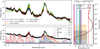 |
Fig. 1 Retrievals of Cassini/VIMS occultation of Titan. Top left: observations and best-fit TAUREX retrievals. Bottom left: breakdown of the extinction contributions in the tholin + CH4(l) (HITRAN) case. Right: atmospheric properties inferred for the tholin + CH4(l) (HITRAN) case. The source for the opacity data (i.e., HITRAN or ExoMol) is important and can slightly change the best-fit spectrum and retrieval interpretation. Overall, the Cassini data is dominated by molecular absorption from CH4, CO, C2H6, and C3H8, as well as from extinction by hydrocarbon aerosols (tholins + CH4(l)). The shape of the 3.4 μm absorption feature is likely best explained by the contribution of multiple species including some contribution from tholins. Overall, retrieval interpretations of Titan’s atmosphere are compatible with stratospheric inferences from previous studies (see Figure B.1). |
4 Applications to JWST exoplanets
For HAT-P-18 b, WASP-39 b and WASP-96 b, we consider the data obtained by the JWST/NIRISS instrument. For WASP-107 b, we consider the data obtained by HST/WFC3, JWST/NIRSpec-G395H, JWST/NIRCam-F322W2, JWST/ NIRCam-F444W and JWST/MIRI. We detail our retrieval results in the next sections.
4.1 Aerosol scattering slopes: Example from HAT-P-18 b, WASP-39 b, and WASP-96 b JWST/NIRISS observations
For HAT-P-18 b, WASP-39 b, and WASP-96 b, results of our retrievals using the L13 aerosol model are shown in Figure 2. We here focus on the L13 retrievals since the posterior distributions for PYMIESCATT retrievals (see the HAT-P-18 b case in Figure C.1) are independent from the assumed cloud composition when using JWST/NIRISS data alone. Similarly, complex terminator modeling (i.e., two distinct regions) is not presented as they did not lead to improved Bayesian evidence over the simpler retrievals. Figure C.2 shows a breakdown of the contributions for the FRECKLL retrievals. Figure C.3 shows the corner plots and computed elemental ratios from both free and FRECKLL runs. The retrieved quantiles of our retrievals are available in Table C.1. The three planets have a roughly similar equilibrium temperature and consistent retrieved T - p structures that are crossing the same condensate curves. However, Figure 2 clearly shows spectra with different shape, suggesting disparate chemistries and cloud structures. We here describe our retrieval findings.
In HAT-P-18 b, we detect the spectral signatures of H2O, CH4, CO2, and Na. The Na abundance is consistent between our free and FRECKLL retrievals with log(Na) — 4.5 (about 10x solar). However, the metallicity of the atmosphere depends on the chemical model, with for instance a recovered log(H2O) ∈ [-4.45, -3.76] dex corresponding to a depleted (Z ~ 0.17x solar) atmosphere for the free retrieval, while the FRECKLL retrieval recovers Z ~ 10x solar metallicity. The metallicity inferred in the free run, from C and O species as well as the refractories (including Na and K), might not be very accurate due to missing species in this estimate. The C/O from the FRECKLL retrieval is estimated to C/O ~ 0.9, while the free retrieval estimate for C/O is much lower and difficult to interpret since major reservoirs of C (e.g., CH4, and CO) are not detected. In general, we caution against over-interpreting C/O computed from the free abundance retrieval, as many C-bearing species are not constrained by the data and because O can easily be sequestered in, for example, other species or aerosols (Fonte et al. 2023). Note that the FRECKLL retrievals used the reduced scheme of Venot et al. (2020), most certainly missing processes (i.e., photochemistry) that are efficiently removing CH4 from the upper atmosphere and could bias the results if mixing is important and the deeper atmosphere is affected: transit data in the near-IR typically probe the 105-100 Pa deeper regions (Caldas et al. 2019; Changeat et al. 2019; Rustamkulov et al. 2023; Feinstein et al. 2023). The detection of Na - which originates from an apparent enhanced absorption at the blue end of the spectrum in the red wing of the 0.6 μm Na line - is a difficult feature to reproduce with the aerosol models used here. We, therefore, note the precarious nature of this detection (and abundance constraints), which relies on very few data points and could also be impacted by instrumental systematics. For the cloud solutions, while the retrieved altitudes for the layers are slightly different between the two runs, they are consistent with a thin layer of sub-micrometer sized particles extending above 1 mbar and extending across the full terminator limb (i.e., Flee consistent with 1). Salt clouds (i.e., KCl, Na2 S, and ZnS are likely contenders as shown in Figure 2: the retrieved T - p profiles cross the condensation lines for these species, but we are unable to distinguish a most likely candidate from the data alone. This is shown in Figure C.1, where the solutions of three retrievals using the TAUREX-PYMIESCATT parameterization with KCl, Na2 S, and ZnS refractive indexes, respectively, lead to the exact same posteriors and evidence. The figure also demonstrates the stability of our solution to the cloud type assumptions and justifies the use of a simpler model (i.e., Lee et al. 2013) for our main conclusions with NIRISS. The formation of KCl or Na2 S clouds should have a significant impact on the gaseous abundances of K or Na, respectively. In particular, gaseous K is constrained to low abundances by this HAT-P-18 b data with log(K) < -9, which could suggest sequestration of K in KCl clouds. However, since gases and condensates are included separately in our inversions, we cannot verify this statement. Complementary, self-consistent approaches connecting gas and condensed phases, as in Ormel & Min (2019); Ma et al. (2023); Arfaux & Lavvas (2024), are needed to properly assess this hypothesis - and, more generally, to invert cloud types from the NIRISS data. Similar results were found for WASP-39 b and WASP-96 b. The abundance constraints of our free run are similar to those from Fournier-Tondreau et al. (2024) despite not accounting for potential light-source effects. CH4, however, was not detected in their study but was here found to similar levels in Fu et al. (2022).
For WASP-39 b, we detect the spectral signatures of H2O, CO, CO2, Na, and K. The atmosphere is here consistent with superstellar metallicity - log(Z) ~ 5× solar for the FRECKLL run and log(Z) ~ 20× solar for the free run. This is mainly due to high water abundance (up to 2.3% in the free run), which is interesting given the subsolar O/H of the host star. We also infer a subsolar C/O ratio, with C/O ~ 0.35 for the FRECKLL retrieval, but as with HAT-P-18 b, we caution against over-interpreting the C/O derived from free retrievals. Both Na and K seem to have significantly enhanced abundances (between 10x and 100x solar depending on the run) with clear spectral signature in the NIRISS spectrum, but this does not seem degenerate with the aerosol solution in this case. Those results are overall consistent with other studies of this dataset (Feinstein et al. 2023; Constantinou et al. 2023; Arfaux & Lavvas 2024). Using the L13 model, clouds are found at high altitude (p < 0.1 mbar) and made from sub-micrometer sized particles. While the retrieved T - p profile is on average hotter than for HAT-P-18 b and does not cross the KCl and ZnS condensation lines (i.e., this could favor Na2S as a possibility for the clouds), the phenomenological properties of the retrieved aerosols are similar to those of HAT-P-18 b. A recent study (Arfaux & Lavvas 2024) employing more complex haze and cloud microphysics has also suggested Na2S as a good contender for the clouds on WASP-39 b. However, their study also indicates that the formation of such clouds would deplete atomic Na in gas, which seems contradictory with the findings from our retrievals. Further iterations between first principle and data oriented approaches are needed here. Recently, a study (Ma et al. 2025) has also performed atmospheric retrievals on the full WASP-39 b data, discussing the possibility of important Si chemistry to explain various spectral features seen at longer wavelengths. These disparate results highlight the need for observations covering a large wavelength range - necessary to break the chemical-cloud degeneracies for exoplanets in this regime - and iterations between free retrieval approaches and self-consistent modeling. We discuss the advantage of the wide wavelength coverage in the next section for WASP-107 b.
In WASP-96 b, we detect signatures of H2 O, CO, Na, and K. Both retrievals (free and FRECKLL) suggest a clear atmosphere. Although this appears to contradict the final interpretations of Taylor et al. (2023) with the same raw data (but not the same reduction), we note that they also find that such a clear solution can fit their data. In our work, the NIRISS spectrum of WASP-96 b is the only one that can be fit with a model that does not include clouds nor hazes. Note that we also performed a tholin retrieval to simulate high altitude hazes but this was also not favored. Interestingly, a cloud-free atmosphere is in line with prior interpretations of the HST and VLT data (Nikolov et al. 2018; Yip et al. 2021). We note that the spectra used in Taylor et al. (2023) were reduced in Radica et al. (2023), but we could not find these resources to conduct further comparisons. In Holmberg & Madhusudhan (2023) - our original source for the WASP-96 b NIRISS spectrum - they did not perform atmospheric retrievals to support their interpretation, but highlighted that assumptions on the stellar limb-darkening have a significant impact on the blue-ward slope (where most of the cloud constraints originate from). Alternatively, we also stress that past observations showing a clear atmosphere might not be fully relevant for the interpretation of JWST data since hot-Jupiters like WASP-96 b are expected to be temporally variable: they could for instance have transient cloud coverage (Skinner & Cho 2022; Changeat et al. 2024). Either way, the spectrum of WASP-96 b presents a blue-ward slope favoring a solution with high abundances of Na and K in our retrievals. The large wings of those atomic species could easily explain the increased absorption in the data from Holmberg & Madhusudhan (2023), and this interpretation is independent from our chemical assumptions (free vs. FRECKLL). In our runs, the metallicity is consistent with slightly subsolar to solar, log(Z) ~ 0.5 × solar for the FRECKLL run and log(Z) ~ 4 × solar for the free case. The only C-bearing species to be detected is CO, potentially suggesting higher than solar abundances of this molecule - C/H ~ 4x solar in the free case - which could explain the inferred super-solar C/O ratio for the free run. However, robust estimates of C/O ratios from free runs might require constraints on multiple carbon species, which, we note, is not achieved here for any of our targets. The FRECKLL retrieval instead suggests a solar C/O ratio. As previously said, Na and K are used by the retrieval to explain the blue-ward slope of our retrievals, which translates into a retrieved super-solar abundance for those species, log(Na) ~ 100 × solar, and log(K) ~ 25 × solar (see the values in Table C.1). Comparing the retrieved T - p profiles with cloud condensation lines (see Figure 2, we expected clouds to be detected as in HAT-P-18 b and WASP-39 b, and similarly to what is favored in Taylor et al. (2023). These different interpretations likely originate from model degeneracies between Na/K and cloud scattering slopes, and/or have contribution from instrumental origin (Taylor et al. 2023; Rotman et al. 2025).
For aerosols, JWST/NIRISS gives access to scattering processes by probing the blue-ward absorption slope of scattering particles at λ < 1 μm. However, in the cases investigated here, the wavelength coverage is not sufficient to identify the type of particles responsible for the enhanced absorption (see, e.g., Figure C.1). The inferred properties, however, seem robust to assumptions on the cloud type, potentially allowing us to safely utilize phenomenological models such as L13. Interestingly, the case of WASP-96 b - which visually shows an increased absorption at blue wavelengths - reveals some level of degeneracies with Na and K continuous wing absorption. For this case, aerosols are not needed to explain the spectrum. For all three targets our self-consistent chemical approach (i.e., FRECKLL) requires some form of disequilibrium processes marked by the retrieved vertical mixing (Kzz > 107 cm2 s-1), despite relatively high equilibrium temperatures. Other processes such as photochemistry - not included in this study - could also play a significant role and bias our interpretations. Retrieval sensitivity and their modeling assumptions should therefore be carefully tested to ensure robust constraints with JWST.
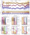 |
Fig. 2 Results of the atmospheric retrievals using the Lee et al. (2013) cloud model for the NIRISS observations. The observed spectra, best-fit models (free chemistry in blue and FRECKLL chemistry in purple), and residuals for the FRECKLL retrieval are shown in the top panel. The lower panels show the retrieved T - p profiles and chemistry - free chemistry in middle row and FRECKLL chemistry in bottom row - with 1 σ confidence intervals, as well as the best-fit aerosol solutions. We also indicate the relevant cloud condensation curves from Wetzel et al. (2013); Gao et al. (2021) with dashed lines for context. Retrieved atmospheric properties are not always fully consistent despite similar Bayesian evidence. The accompanying posterior distributions of these retrievals are available in Fig. C.3. |
4.2 Silicate aerosol feature: WASP-107 b observations
For WASP-107 b, recent studies (Dyrek et al. 2024; Welbanks et al. 2024; Sing et al. 2024) have employed atmospheric retrievals and grid model fits to interpret the observations. Welbanks et al. (2024) is the only study to date to have performed retrievals of the full dataset (including HST and MIRI data), so we make a more direct comparison with their results7. We note that they did not include cloud properties directly and instead modeled the 10 μm silicate Si-O stretch feature using a Gaussian-like extinction. Here, we aim to constrain the type of clouds present in WASP-107 b’s atmosphere, so we use TAUREX-PYMIESCATT to compute the extinction of various possible species: SiO, SiO2, MgSiO3, and Mg2SiO4. This is a significant departure from their study. The results of our retrievals, including spectra, T - p structures, and probability distributions for the free parameters, are shown in Figure 3. In Table C.2, we provide the quantiles from our different retrievals. Many of our results are consistent within the models and datasets we consider: detection of H2O, SO2, CH4, CO, and CO2, and presence of high-altitude (p < 104 Pa) clouds composed of sub-micrometer SiO2 particles. Other results, however, are model or dataset-dependent, which is explained below.
In the retrievals assuming free chemistry, the metallicity is subsolar: log(H2O) ~ -4 dex. On the contrary, the FRECKLL chemistry retrievals favors a super-solar metallicity: Z ∈ [20,50]x solar. Note again that the FRECKLL retrievals do not include S-species and photochemistry (use of reduced scheme); therefore, the SO2 production described by Polman et al. (2023); Tsai et al. (2023); Dyrek et al. (2024) is not included. The differences between free and self-consistent chemistry for this planet are likely driven by the red end of the MIRI data, which cannot be easily fit using the less flexible FRECKLL retrievals. This is either because of the added chemical constraints from the model, or because of our assumption of 1D aerosols. Regarding the latter point, our free chemistry runs allow for scattered clouds to exist - we find a cloud fraction of Fa ∈ [0.4,0.5] -while the FRECKLL runs do not. Retrieving the type of particles is possible (but challenging) due to the clearly visible 10 μm Si feature, and as illustrated by Figure C.5. In all our retrievals, SiO2 clouds composed of sub-micrometer particles (μ < 0.7 μm) are detected. This is because the Si-O feature starts from 8 μm, which can only be matched by the SiO2 clouds in our model. Except for the (FRECKLL) retrieval with NIRSpec, these SiO2 particles are also responsible for the gray opacity at lower wavelengths (i.e., in the HST data), however, the broader Si-O feature extending up to 11 μm requires an additional component. In these retrievals, small (μ < 0.1 μm) MgSiO3 particles located above the SiO2 clouds can play this role. Processes that would lead to the formation of such cloud structures at the terminator of hot-Jupiters remains to be modeled self-consistently and are outside the scope of this work. In the NIRSpec (FRECKLL) run, the solution is different: the retrieval finds that a larger quantity of much smaller SiO2 particles (μ ~ 0.02 μm) mixed with ~ 0.5 μm Mg2SiO4 particles could also work well. In this case, the visiblelight continuum is best explained by the Mg2 SiO4 particles with SiO2 contributing only to the enhanced absorption at ~8 μm as seen in Figure C.5. These degeneracies highlight the difficulties in extracting robust constraints for exoplanet aerosols, especially as many possible particle shape and types can contribute to the shape of the 10 μm Si feature (see discussion). For instance, a study focusing on the HST+MIRI data only (Dyrek et al. 2024) explained the Si-O feature using SiO clouds only (see their ARCIS retrievals), albeit with some results where SiO2 clouds are favored (see their PETITRADTRANS retrievals). Independently, Si-based condensates, likely including SiO2 particles, are found by all the retrievals run in our study (and also other works: Dyrek et al. 2024; Welbanks et al. 2024; Sing et al. 2024). The retrievals suggest that these Si-clouds are located above their respective condensation points (see Figure 3), which remain difficult to explain without invoking significant particle transport. In particular, the free retrievals show high altitude clouds (i.e., p < 10 Pa) while the retrieved thermal profiles are inverted, crossing the condensation curves of silicates again (see Figure 3). In this situation, sublimation of the cloud particles should efficiently remove clouds, which appear inconsistent with our findings. In the FRECKLL retrievals, the thermal inversion is not present but a hotter internal temperature seems needed, which was also suggested by the previous works of Welbanks et al. (2024); Sing et al. (2024). In this case, the silicate condensation curves are crossed around p ~ 0.1-1 bar, and significant mixing is still needed to lift the particles up to the region probed by the observations. This could be consistent with the retrieved vertical mixing of Kzz ~109 cm2 s-1, which is constrained by the disequilibrium chemical profiles. Other aspects not modeled here, including a more complex 3D structure at the terminator could play a significant role and further bias our inference (Caldas et al. 2019; Changeat & Al-Refaie 2020; MacDonald et al. 2020; Lacy & Burrows 2020a). Note that our free chemistry results contrast with the interpretations from Dyrek et al. (2024); Welbanks et al. (2024), where we find a lower abundance for most of the molecules, while our FRECKLL retrievals are consistent.
Another interesting finding of our study is the difference in solutions extracted from the NIRCam and NIRSpec datasets. The retrieved molecular abundances of the detected species in both dataset combinations can vary by up to ±1 dex. For NH3, however, the molecule is only detected when NIRCam is included. For H2 S, it is only detected when NIRSpec is included. These differences arise from incompatible spectral shape between the NIRCam-F322W2 and the NIRSpec-G395H NRS1 spectra (see Figure C.4), with the NIRCam data being steeper than the NIR-Spec data at λ < 3.7 μm. This could be explained by temporal variability of the planet’s atmosphere (e.g., variability in the aerosol layers), but it is most likely due to systematic differences in the observing conditions (i.e., light-source effects: Sing et al. 2024) and/or the reduction of the data. Differences such as offsets have also been identified in recently analyzed observations of WASP-39 b (see, e.g., Lueber et al. 2024; Carter et al. 2024), while other studies have highlighted significant and poorly understood, wavelength-dependent, long-term trends in NRS1 light-curves (Espinoza et al. 2023). Recent works (Moran et al. 2023; Edwards & Changeat 2024) have also suggested that systematic offsets could occur between the NRS1 and NRS2 detectors (here, we do not fit systematics between the two detectors). Presence of those instrumental systematic signals can introduce biases, at minimum in the form of offsets, raising caution in interpreting combined datasets (see: Edwards et al. 2024). For reference, our retrievals find offsets between HST, NIRSpec, NIRCam, and MIRI data of up to 250 ppm. Our results suggest that a large wavelength coverage is necessary to break the degeneracies between chemical and aerosol signatures, but also provides clues about the difficulties of combining JWST datasets.
Our retrieval exploration of the WASP-107 b data suggests that interpretations of current JWST data can be subject to various biases. Some of those biases were clearly highlighted in this paper: choice of input data (cross-sections, aerosol optical properties), observations (i.e., wavelength coverage, data reduction), and importantly model assumptions (free vs. self-consistent chemistry, aerosol modeling). We explore some of these aspects further in the next section.
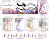 |
Fig. 3 Summarized results of the retrievals on the WASP-107 b HST and JWST data. The top left panel shows the observed spectra corrected for offsets for the FRECKLL retrievals (data points), the best fits of the free and FRECKLL retrievals (solid lines), and the contributions from the FRECKLL HST+NIRCam+MIRI retrieval (shaded areas). The top right panel shows the retrieved thermal structures including 1 σ and 3 σ confidence regions (shaded areas), as well as the cloud condensation curves from Wetzel et al. (2013); Gao et al. (2021); Grant et al. (2023). The middle row shows the chemistry and aerosol structure (SiO2, MgSiO3, and Mg2SiO4) for the four retrievals. The bottom row shows the retrieved probability density. The metallicity (Z) is directly retrieved from the FRECKLL retrievals but estimated from the O/H (normalized by WASP-107 value) in the free retrievals. Overall, the atmosphere of WASP-107 b is consistent with high-altitude Si-clouds, but the exact solution somewhat depends on the considered data (NIRSpec or NIRCam) and model assumptions. Figure C.4 shows the incompatibility of the NIRSpec and NIRCam spectra, leading to slightly different solutions. |
5 Discussion
We provide specific examples of cloud and haze retrievals with real JWST data. However, to build a more general intuition of the telescope’s information content, additional controlled simulations are required. We utilize a synthetic hot Jupiter scenario based on the WASP-107 b parameters. The atmosphere is assumed to be at chemical equilibrium (Woitke et al. 2018) with a 20 × solar atmosphere to which we add 10 ppm of SO2. This is motivated by recent JWST measurements for this planet (Dyrek et al. 2024; Welbanks et al. 2024; Sing et al. 2024). A 10Pa aerosol layer of MgSiO3 is added using an exponentially decaying profile with χmax = 105 particles/m3 and the Budaj et al. (2015) distribution with μr = 0.5 μm. In Forward Model 1 (FM1), the particles are assumed spherical. In FM2, the particles have a porosity of 0.5 (see Appendix A). Following the methodology in Changeat et al. (2019), the TAUREX highresolution spectrum from FM1 and FM2 are convolved with JWST instrument noise models (Batalha et al. 2017) for NIRISS-SOSS, NIRSpec-G395H, and MIRI-LRS using the instrument-recommended setups (using 3, 15, and 41 groups, respectively). Five retrieval cases are then investigated:
Case 1a: Baseline with spheres. It includes MgSiO3 and SiO2 clouds using spherical particles to test the feasibility of distinguishing aerosol species (i.e., it is a self-retrieval for FM1, but it was also attempted on FM2 to test the importance of the spherical particle assumption).
Case 1b: Baseline with porous particles. It includes MgSiO3 and SiO2 clouds using porous particles to test the feasibility of distinguishing aerosol species and their porosity with the FM2 spectrum (i.e., it is a self-retrieval for FM2).
Case 2: SiO2-only. Same as Case 1a but without MgSiO3 clouds. This case evaluates biases from using incorrect refractive indexes.
Case 3: Lee clouds. Same as Case 1a but using L13 prescription.
Case 4: constant χ. Same as Case 1a but with a constant-with-altitude particle number density instead of the exponentially decaying profile.
Case 5: log-normal particle size. Same as Case 1a but assumes a Log-Gaussian particle distribution n(r).
Note that only Case 1b uses porous particles, while all the other cases assume spherical particles. Those cases are specifically designed to test the sensitivity of JWST to various important cloud properties. Since the full set of JWST observations (i.e., from λ ∈ [0.8,12] μm) are not always available, or because temporal variability could render the datasets incompatible (Cho & Polvani 1996; Cho et al. 2003; Skinner et al. 2023; Changeat et al. 2024), we also produce Case 1a, Case 2, and Case 3 for the NIRISS+NirSpec data only and the MIRI data only. Figure 4 shows the simulated data and retrieved spectra, while the corner plots for relevant cases are available in Figure D.1.
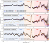 |
Fig. 4 Simulated observations and retrieval best-fit models of our controlled experiments. The top panel shows retrievals on the full simulated spectrum with JWST/NIRISS, JWST/NIRSpec-G395H, and JWST/MIRI. The middle panel shows retrievals on subsets of the simulated data. Both panels use the FM1, where aerosol particles are spherical. The bottom panel shows retrievals on the FM2, where aerosol particles are 50% porous. This ensemble of simulations (and corresponding posterior distributions in Figures D.1 and D.2) illustrates the need for a wide wavelength coverage to constrain aerosol properties accurately. Retrievals restricted to a narrow wavelength coverage (NIRISS+NIRSpec) or (MIRI) are at risk of biases, especially when using incorrect refractive indexes (properties that are a priori poorly known). Porosity is difficult to infer from JWST data (even when using the full dataset), as it is degenerate with other parameters (i.e., models using spherical particles can achieve good fits). |
5.1 Biases from assuming incorrect aerosol types
Without prior knowledge from theoretical modeling, assuming incorrect cloud type could lead to retrieval biases. Comparing the baseline (Case 1a) and SiO2-only (Case 2) cases, we conclude that incorrect refractive indexes or missing cloud species in retrievals generally lead to wrong inference of the chemistry, thermal structure, and cloud properties. Importantly, this issue (i.e., using the wrong refractive indexes) is only visible in the fit when the full wavelength coverage is available. When using the NIRISS+NIRSpec data only or the MIRI data only, the recovered parameters are incorrect - for instance Z is about 10σ off in the NIRISS+NIRSpec case, while log(SO2) is 4σ off in the MIRI-only case - but the best-fit spectra in the region of the observations remain very similar. Due to this behavior, narrow wavelength coverage (i.e., when simultaneous visible and infrared data is not available) should be interpreted with caution when prior knowledge on the cloud composition is not available. However, we note that a more heuristic approach (e.g., Case 3 using L13) can be adapted when strong cloud absorption features are not present in the data (e.g., in the JWST/NIRISS cases studied in Section 4), leading to robust, unbiased results. For instance, the Case 3 L13 retrieval on NIRISS+NIRSpec obtains unbiased chemical parameters and relevant cloud properties: Z = 22 ± 2, C/O = 0.50 ± 0.05, log(SO2) = -4.9 ± 0.1, log(P) = 1.00 ± 0.06, log(μr) = -1.0 ± 0.5. This is in line with the findings of Section 4 on the NIRISS data.
5.2 Aerosol particle shape assumption
Recent studies suggested the potential importance of particle porosity in interpreting atmospheric observations of exoplanets (Adams et al. 2019; Ohno et al. 2020; Samra et al. 2020; Lodge et al. 2024; Vahidinia et al. 2024). In our examples, we assumed for simplicity that the aerosol particles are filled and spherical. Previous works (Fabian et al. 2001; Min et al. 2007; Kataoka et al. 2014; Kiefer et al. 2024) have demonstrated significant changes in extinction when more complex particle shapes (e.g., porous spheres, distribution of particles) are assumed. To illustrate such difficulties, we tested Case 1b, which is the same as Case 1a but with porous particles. Figures 4 and D.2 show how this assumption impacts the forward model spectra (compare FM1 and FM2). The retrievals assuming spherical particles are able to explain the FM2 spectrum (when porous particles are in the forward model) convincingly, but the retrieved parameters are biased: the particles size and number density is incorrect, which also impacts the retrieved metallicity (Z). Intrinsic degeneracies exist, making it difficult to extract particle porosity. Such issues are also likely to occur when it comes to the particle arrangements (e.g., amorphous, crystalline), potentially leading to significant challenges in our ability to interpret the 10μm feature of silicate clouds in hot Jupiters.
5.3 Cloud information content in JWST data
Comparing Case 1a to cases 4 and 5, we can evaluate the sensitivity of JWST to the vertical aerosol profile and particle radius distribution. Case 4 (when χ is constant with altitude) does not display significant differences compared to our baseline scenario, highlighting the poor sensitivity of WASP-107 b-like data to vertical aerosol profile. In Case 5, however, we attempt to recover the particle size distribution directly, assuming it is normally distributed. We find in Figure D.1 a very strong inverse linear correlation between the posterior distributions of μc and σc in log space. The correlation indicates that the radiative contributions of aerosols in transit geometry are dominated by the largest particles of the distribution (i.e., information on the full distribution and its shape is redundant). From our results, detailed estimates of the vertical aerosol distribution and the particle size distributions seem difficult with JWST, meaning that simplified parameterizations for those factors might be sufficient to capture most of the available information.
5.4 Synergies between microphysical cloud models and information retrievals
In this study, we quantify the sensitivity of JWST to particular properties of aerosols. For instance, we unveil that the actual particle radius distribution and the vertical aerosol abundance are second order properties affecting the observed spectra, and could be simplified or parameterized when comparing with current observations. This is important information as for teams developing complex microphysical cloud models (e.g., Helling et al. 2008; Ohno & Okuzumi 2018; Gao & Benneke 2018; Powell et al. 2018; Ohno et al. 2020; Samra et al. 2022; Lee 2023; Powell & Zhang 2024) this allows us to more easily identify the properties that could affect observables. Similar efforts have already been conducted for chemical properties (Changeat et al. 2019; Al-Refaie et al. 2022, 2024), or planetary mass (Changeat et al. 2020b), providing relevant guidelines for parameterization and modeling in atmospheric retrievals. In this context, the development of information oriented approaches (i.e., free retrievals) should idealistically be done in conjunction with self-consistent approaches, with iterations until both techniques agree (i.e., the model complexity is adapted, and our current knowledge of physical processes is correct). Research on aerosols is only beginning, motivated by recent access to high-quality data (i.e., JWST) and recent advancements in self-consistent cloud models for retrieval applications (Ormel & Min 2019; Min et al. 2020; Ma et al. 2023). For chemistry, differences between our free and FRECKLL retrievals potentially highlight that such a level of agreement has not yet been reached for chemical models relevant to JWST data.
6 Conclusion
In this work, we parameterized cloud and haze properties to explore the information content of JWST exoplanet spectra. We first evaluated the strategy on a Solar-system example of Titan, observed in occultation by the Cassini spacecraft. We then performed similar atmospheric retrieval tests on recent JWST exoplanet data from the JWST/NIRISS and the JWST/MIRI instruments. We explored various retrieval assumptions using the TAUREX3 retrieval code. Notably, we performed retrievals beyond the common chemical equilibrium assumption using the kinetic chemistry code FRECKLL on JWST data for the first time. Our findings, also supported by additional controlled experiments using simulated data, confirm that characterizing the physical properties of aerosols (i.e., understanding their nature, size distribution, and abundances) requires a wide wavelength coverage, as also suggested in other studies (see, e.g., Lee et al. 2014; Wakeford & Sing 2015; Pinhas & Madhusudhan 2017; Mai & Line 2019; Kawashima & Ikoma 2019; Lacy & Burrows 2020b; Gao et al. 2021). Specifically, to minimally constrain aerosols, observations need to be sensitive to both the visible light scattering slope and longer wavelength resonance features (e.g., the 10 μm Si-O stretch). Without the combined information from these spectral regions - and in absence of further priors - the aerosol solution can be degenerate and easily lead to incorrect conclusions. Breaking this degeneracy with JWST alone may be a complicated task, since the telescope does not possess an instrument covering those wavelengths simultaneously. When attempting to combine observations from different epochs to construct such a wavelength coverage, we note incompatibilities in the data (i.e., WASP-107 b NIRSpec and NIRISS) that might prevent us from using this strategy efficiently. Possible sources of these discrepancies include the time dependence of the observing conditions (i.e., changing instrument systematics and stellar variability) and/or the time dependence of the astrophysical signal itself (exoplanet weather). To make further progress in this area, we suggest that synergies with other instruments (HST, ground-based, and Ariel) should be explored to provide the required simultaneous coverage and mitigate the biases from repeated visits. Our investigations also highlight important retrieval challenges inherently linked to modeling assumptions (i.e., free chemistry versus kinetic chemistry and aerosol model assumptions) and the assumed input sources (cross-sections and aerosol optical data).
Data availability
The atmospheric retrieval code TAUREX3 is open source and available at: https://github.com/ucl-exoplanets/TauREx3. The TAUREX3 plugins developed and used for this article are also publicly available on Github: TAUREX-PYMIESCATT at https://github.com/groningen-exoatmospheres/taurex-pymiescatt, TAUREX-MULTIMODEL at https://github.com/groningen-exoatmospheres/taurex-multimodel, and TAUREX-INSTRUMENTSYSTEMATICS at https://github.com/groningen-exoatmospheres/taurex-instrumentsystematics. The opacity sources that were compiled for this article are compatible with the TAU-REX3 framework and can be found in a Zenodo repository: https://doi.org/10.5281/zenodo.15495830.
Acknowledgements
We thank the anonymous referee for their useful comments that significantly improved our manuscript. This publication is part of the project “Interpreting exoplanet atmospheres with JWST” with file number 2024.034 of the research program “Rekentijd nationale computersystemen” that is (partly) funded by the Netherlands Organisation for Scientific Research (NWO) under grant https://doi.org/10.61686/QXVQT85756. This work used the Dutch national e-infrastructure with the support of the SURF Cooperative using grant no. 2024.034. D.B. and O.V. acknowledge funding from Agence Nationale de la Recherche (ANR), project “EXACT” (ANR-21-CE49-0008-01). We also acknowledge the availability and support from the High-Performance Computing platforms (HPC) from DIRAC, and OzSTAR, which provided the computing resources necessary to perform this work. This work utilized the Cambridge Service for Data-Driven Discovery (CSD3), part of which is operated by the University of Cambridge Research Computing on behalf of the STFC DiRAC HPC Facility (www.dirac.ac.uk). The DiRAC component of CSD3 was funded by BEIS capital funding via STFC capital grants ST/P002307/1 and ST/R002452/1 and STFC operations grant ST/R00689X/1. DiRAC is part of the National eInfrastructure. This work utilized the OzSTAR national facility at Swinburne University of Technology. The OzSTAR program receives funding in part from the Astronomy National Collaborative Research Infrastructure Strategy (NCRIS) allocation provided by the Australian Government. This work is based upon observations with the NASA/ESA/CSA James Webb Space Telescope, obtained at the Space Telescope Science Institute (STScI) operated by AURA, Inc. The raw data used in this work are available as part of the Mikulski Archive for Space Telescopes. We are thankful to those who operate these telescopes and their corresponding archives, the public nature of which increases scientific productivity and accessibility (Peek et al. 2019).
Appendix A Plugin additions to TAUREX3
In this appendix, we describe the three new plugins TAUREX-PYMIESCATT, TAUREX-MULTIMODEL and TAUREX-INSTRUMENTSYSTEMATICS.
A.1 Aerosol modeling with TAUREX-PYMIESCATT
For this work, a novel TAUREX3 plugin, TAUREX-PYMIESCATT is developed. The code is designed to model and retrieve parameterized aerosol properties, for application to exoplanet data. For each aerosol species, the plugin uses the python library PYMIESCATT (Sumlin et al. 2018) to estimate the Mie Extinction Efficiency (Qext), and cross-sections, of spherical particles from their complex refractive index8: m = x + iy. Since Qext is computed for a single homogeneous sphere, the contribution from poly-dispersed particles is estimated by weighting sampled points of the particle size distribution. Following Pinhas & Madhusudhan (2017), the available particle size distributions (n) in TAUREX-PYMIESCATT are:
1) Log-Normal distribution:
 (A.1)
(A.1)
where r is the sampled particle radius, μr is the mean particle radius, and σr is the scale of the particle size distribution.
2) Modified Gamma distribution (Deirmendjian 1964):
 (A.2)
(A.2)
where a, b, c, and d are positive coefficients.
3) A particular case of 2) from Budaj et al. (2015):
 (A.3)
(A.3)
where here, μr represents the critical radius for which the function is maximum. As fitting for the full form of the particle size distribution cannot be done with current instruments, the latter distribution provides a convenient single-parameter description of n.
Then, the cross-section σ (in m2), is given by
 (A.4)
(A.4)
where 
The contribution to the optical depth is obtained by multiplying with the particle number density χ (in m-3), which is a function of the altitude z. In exoplanet studies, aerosol layers are often parameterized by a boxcar function, with χ(z) = 0 outside reference bottom and top pressures and χ(z) = χ inside of the reference pressures (i.e., χ is constant in the cloud layer). In TAUREX-PYMIESCATT, this boxcar function for a species S is defined by its mean pressure (PS) and its range (ΔPS, always in log space). Other studies have also suggested an exponential decay with pressure (e.g., Atreya & Wong 2005; Whitten et al. 2008), so this option is also offered in TAUREX-PYMIESCATT, with χ defining the number density at the bottom of the layer and α describing the exponential decay factor. In this case, χ(z) is given by
 (A.5)
(A.5)
where pref is the reference pressure at the bottom of the cloud layer. In TAUREX, contributions can be added dynamically. TAUREX-PYMIESCATT makes use of this feature, allowing multiple cloud layers and species to be added simultaneously.
Since precise calculations of components are difficult, we use Effective Medium Theory (see Bohren & Huffman 2008; Kataoka et al. 2014) to calculate the refractive index of porous particles and aggregates. In TAUREX-PYMIESCATT, the modified refractive indexes can be computed using the Brugge-man mixing rule (Bruggeman 1935) or the Maxwell-Garnet mixing rule (Maxwell-Garnett 1904). In this work, we focus on spherical particles, but include a retrieval example with porous particles in Section 5.
TAUREX-PYMIESCATT also provides an implementation of the phenomenological aerosol model from Equation (A1) of Lee et al. (2013): it uses the same equations as already available in the base TAUREX code but reformulates the parameterization to be consistent with the PYMIESCATT implementation. In this model, Qext is inferred from an empirical fitting function rather than Mie theory The formulation does not use complex refractive indexes from aerosol species, so it cannot account for resonance (i.e, spectral feature), but it provides a simpler and more generic alternative for featureless aerosol absorption (see Section 2.3.2 in the original paper). The free parameters in this model are the similar to the PYMIESCATT model: particle size (μr), the extinction reference radius (Q0), the particle number density (χ), and the location of the cloud layer in pressure (labeled Plee for the middle and ΔPlee for the extent of the cloud layer).
In Figure A1, forward models demonstrate the impact of particle types, size and number density on observed spectra.
A.2 Inhomogeneous atmospheres with TAUREX-MULTIMODEL
Recent works have shown the importance of modeling spatial inhomogeneities when interpreting exoplanet atmospheres (Feng et al. 2016; Caldas et al. 2019; Changeat & Al-Refaie 2020; Taylor et al. 2020; MacDonald et al. 2020; Pluriel et al. 2020; Nixon & Madhusudhan 2022). We here introduce a novel TAU-REx3 plugin, TAUREX-MULTIMODEL, which is a mixin (see: Al-Refaie et al. 2022) that enables multiple forward models (or regions) to contribute to the final flux. It is compatible with all the available TAUREX3 forward models. The contribution of each region, denoted i, is controlled by a contribution factor (Fi) between 0 and 1 (the sum of all region contributions is forced to equal 1). In this work, we use TAUREX-MULTIMODEL to add inhomogeneous cloud coverage at the limbs, but we highlight that the plugin is not limited to cloud parameters: all the forward model properties can be retrieved individually (i.e., for each region) or coupled flexibly. The TAUREX-MULTIMODEL plugin also adds the ability to post-process the forward model with an instrument function. Here, the instrument response has a Gaussian profile of width modeled by a polynomial function of λ (the coefficients of the polynomial can be retrieved). This is useful when dealing with the JWST data at pixel resolution since the line spread functions of the JWST instruments are designed to span multiple pixels. This feature is not used in this work since the literature data is provided at much lower resolution than the instrument is capable.
A.3 Treatment of instrument systematics with TAUREX-INSTRUMENTSYSTEMATICS
TAUREX-INSTRUMENTSYSTEMATICS is a small TAUREX3 plugin to handle retrievals of combined datasets. Previous works have shown that combining datasets can lead to inconsistent results when instrument systematics remain present. This was particularly true in the HST era (Yip et al. 2021), when assumptions in the reduction pipelines could lead to significant (i.e., ~500ppm) vertical offsets - with the spectral shape in the data remaining relatively conserved - and, therefore, to widely different interpretations (see a striking example of this for KELT-11 b: Changeat et al. 2020a; Colón et al. 2020; Edwards et al. 2024). Recent works on the ERS data of WASP-39 b have also similar issues for JWST (Constantinou et al. 2023). With TAUREX-INSTRUMENTSYSTEMATICS, we provide retrieval capabilities for the most basic instrument systematics: vertical offsets and linear slopes. More complex systematics could eventually be handled in the future if warranted by the data. Additionally, with TAUREX-INSTRUMENTSYSTEMATICS, each observation can be associated with an instrument response file. The response file is used to describe the shape of the Gaussian profile of the instrument response function (similar treatment to TAUREX-MULTIMODEL), which is then convolved with the atmospheric forward model.
 |
Fig. A.1 Example forward models of WASP-107 b’s atmosphere using various cloud species and compared to MIRI data (black data points) of Dyrek et al. (2024). Left column: Varied number density of the cloud particles, Xc in log part/m3. Right column: Varied particle radius, Rc in μm. The atmosphere is modeled using the T-p profile from Fig. 3 of Dyrek et al. (2024) and equilibrium chemistry, assuming a solar C/O and a 20x solar metallicity. We manually force a constant SO2 mixing ratio of 10ppm to capture the enhanced 8 μm feature. Clouds are parameterized using the exponentially decaying layer and spanning one log pressure scale centered at 10 Pa. It is difficult to distinguish which cloud species is present from observing a narrow wavelength range. |
Appendix B Supplementary data for Titan retrievals
Table B.1 contains the complex refractive index for Tholin used in this study. Figure B.1 shows the posterior distributions from TAUREX retrievals of Cassini Titan’s data.
Refractive indexes for tholins used in this study, computed by interpolating data from Khare et al. (1984); Rannou et al. (2010). See the "Data availability" section to access the full data table.
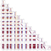 |
Fig. B.1 Posterior distribution for the Cassini/VIMS retrieval of Titan data using the HITRAN cross-sections (red) and the ExoMol cross-sections (blue). The stratospheric hydrocarbon abundances, inferred from other studies, are also shown in orange for ISO/Hershel (Coustenis et al. 2003), in teal for Cassini/CIRS (nominal mission 2004-2010, Coustenis et al. 2010), and in red for Cassini/CIRS (extended mission 2014, Coustenis et al. 2016; Sylvestre et al. 2018). The literature value for CO is from Maltagliati et al. (2015). While slightly different chemical compositions are quoted in the literature - depending on the probed altitudes and observations - overall, the retrieval agrees well with prior knowledge of Titan’s stratosphere. The atmosphere is also consistent with the presence of small (μr ~ 0.2 μm) haze particles extending as high as 0.1 mbar, with a deeper cloud cover (modeled here with CH4 condensates) composed of larger particles (μr ~ 0.4 μm). |
 |
Fig. B.2 Retrieval results of the Cassini/VIMS occultation of Titan, with both the temperature profile and methane retrieved. The reference values in the posteriors are from the same source as in Figure B.1. This setup would be more representative of an exoplanet approach where the priors on the thermal structure and chemistry are unknown. The spectral fit and retrieved chemistry match the results from the main text. However, we obtain inconsistent results for the aerosol solution and the T - p profiles. For the T - p profile, in particular, the retrieved solution does not match the known truth for Titan’s atmosphere. Such degeneracies are expected for exoplanet transit retrievals where obtaining robust T - p structure remains difficult (Rocchetto et al. 2016; Schleich et al. 2024). This is especially true for cases involving secondary and cloudy atmosphere (see e.g., Changeat et al. 2020b; Di Maio et al. 2023). |
Appendix C Supplementary information on JWST retrievals
This section contains supplementary information for the JWST retrievals. Figure C.1 shows the posterior distributions for the HAT-P-18 b NIRISS retrievals using refractive index of KCl, ZnS and Na2S. Figure C.2 shows a breakdown of the relevant opacity contributions to the FRECKLL retrievals of HAT-P-18 b, WASP-39 b, and WASP-96 b. Figure C.3 shows the posterior distributions of the NIRISS retrievals. Figure C.4 shows a zoomed-in version of the data and best fit models for the WASP-107 b retrievals. Figure C.6 shows the posterior distributions of the WASP-107 b retrievals. Lastly, Table C.1 and Table C.2 provide the retrieved properties from our JWST retrievals.
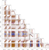 |
Fig. C.1 Posterior distribution for the JWST/NIRISS free retrievals of HAT-P-18 b using various clouds species. Blue indicated KCl clouds; red indicates Na2S; and gold indicates ZnS. The abundances of the chemical species are unchanged by the different types of clouds, likely because JWST/NIRISS probes the scattering slope at visible to near-infrared wavelengths and does not cover cloud spectral features. Similar conclusions were inferred from WASP-39 b and WASP-96 b. |
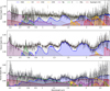 |
Fig. C.2 Contribution of different processes to the transmission spectra of HAT-P-18 b (top), WASP-39 b (middle), and WASP-96 b (bottom) obtained from the FRECKLL retrievals. The contribution from water dominates most of the spectra after 1.2 μm, while short wavelengths are dominated by the broadened lines of Na and K (WASP-96 b), or by aerosols (HAT-P-18 b and WASP-39 b). In HAT-P-18 b, H2O, CH4, CO2 and Na are detected. In WASP-39 b, H2O, CO, CO2, Na, and K are detected. In WASP-96 b, H2O, CO, Na, and K are detected. |
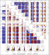 |
Fig. C.3 Posterior distribution for the JWST/NIRISS retrievals of HAT-P-18 b (gold), WASP-39 b (red), and WASP-96 b (blue) using the Lee et al. (2013) cloud model. The bottom left corner plot shows retrieved posterior distributions for the free chemistry retrievals. The top right inverted corner plots show the FRECKLL retrievals. To enable comparison, we also compute (bottom) the elemental ratio probability densities by postprocessing the free chemistry runs. For these, we indicate reference Solar-system values. The values for Jupiter are computed from Atreya et al. (2022); the values for the Sun are from Asplund et al. (2009); and the values for the stars HAT-P-18 and WASP-39 are from the Hypatia catalog (Hinkel et al. 2014). Note that the reference abundances for Na and K in Jupiter are not available, due to the condensation of those species. Here, we estimate those values by using S/H as a proxy for Na and K enrichment (i.e., we assume S is a good tracer of refractory elements). Stellar elemental ratios for WASP-96 are not available. |
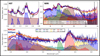 |
Fig. C.4 Spectra and best-fit models for the WASP-107 b study. Red lines indicate the case where the NIRCam data is considered; blue lines indicate the case where the NIRSpec data is considered. We also show the contribution of the different components in the model to the best-fit spectrum for the NIRCam (FRECKLL) case. While the retrieval results are similar, systematic differences exist between the NIRCam and NIRSpec data for λ < 3.7 μm. This difference could be due to remaining instrumental systematics or a time-varying cloud cover. Note that the observations are plotted with the vertical offsets corrected. |
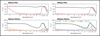 |
Fig. C.5 Contribution (Cclouds) of individual cloud species in the best-fit to the WASP-107 b data normalized by the atmospheric scale height (H = 1030 km), showing the contribution of the individual components. In all our retrievals, SiO2 clouds (in blue) seem necessary to explain the sharp opacity rise at λ > 8 μm. However, they do not explain 100% of the feature requiring secondary contributions from either MgSiO3 or Mg2SiO4 particles. |
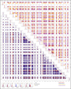 |
Fig. C.6 Posterior distributions of the retrievals on the WASP-107 b data. The bottom left corner plot indicates retrieved posterior distributions for the free chemistry retrievals. The top right inverted corner plot indicates the FRECKLL retrievals. To enable comparison, we also compute (bottom) the elemental ratio probability density by post-processing the free chemistry runs. For these, we indicate reference Solar-system values. The values for Jupiter and the Sun are the same as in Figure C.1. The value for WASP-107 are from Hejazi et al. (2023). |
Retrieved properties from the NIRISS observations of HAT-P-18 b, WASP-39 b, and WASP-96 b using the free and FRECKLL retrievals.
Retrieved properties for the MIRI data of WASP-107 b with our different observational setups and models.
Appendix D Supplementary information for the discussion section
This appendix contains supplementary information regarding the simulations of Section 5. Figure D.1 shows the corner plots of the full retrieval cases with spherical particles (forward model FM1). Figure D.2 shows the corner plots of the full retrieval cases when the forward model contains porous particles (forward model FM2).
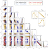 |
Fig. D.1 Posterior distributions of the retrievals from the top panel of Figure 4 (the inset refers to non-shared parameters). The colors are maintained across the figures: black indicates baseline retrieval, blue the SiO2-only retrieval, red the constant cloud retrieval, and gold the Gaussian particle distribution retrieval. The SiO2-only retrieval shows that a large wavelength coverage allows us to distinguish aerosol properties. The other retrievals indicate that this dataset is poorly sensitive to the vertical aerosol abundance distribution, but that the size of the largest particles in the distribution can be recovered (see the negative correlation between the mean and the variance of the Gaussian distribution). |
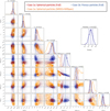 |
Fig. D.2 Posterior distributions of the retrievals from the bottom panel of Figure 4 (the inset refers to non-shared parameters). The colors are maintained across the figures: red indicates the spherical particles (Full), orange the spherical particles (NIRISS+NIRSpec only), and blue the porous particles (Full). Retrieving the porosity of aerosol particles is difficult with JWST data, as indicated by the fit obtained from the spherical particle retrieval in the bottom panel of Figure 4. The model compensates by introducing a bias in the particle size and abundance, but the chemistry remains similar. |
References
- Abel, M., Frommhold, L., Li, X., & Hunt, K. L. 2011, J. Phys. Chem. A, 115, 6805 [NASA ADS] [CrossRef] [Google Scholar]
- Abel, M., Frommhold, L., Li, X., & Hunt, K. L. 2012, J. Chem. Phys., 136, 044319 [NASA ADS] [CrossRef] [Google Scholar]
- Ádámkovics, M., Mitchell, J. L., Hayes, A. G., et al. 2016, Icarus, 270, 376 [Google Scholar]
- Adams, D., Gao, P., de Pater, I., & Morley, C. V. 2019, ApJ, 874, 61 [NASA ADS] [CrossRef] [Google Scholar]
- Al Derzi, A. R., Furtenbacher, T., Tennyson, J., Yurchenko, S. N., & Császár, A. G. 2015, JQSRT, 161, 117 [Google Scholar]
- Al-Refaie, A. F., Changeat, Q., Waldmann, I. P., & Tinetti, G. 2021, ApJ, 917, 37 [NASA ADS] [CrossRef] [Google Scholar]
- Al-Refaie, A. F., Changeat, Q., Venot, O., Waldmann, I. P., & Tinetti, G. 2022, ApJ, 932, 123 [NASA ADS] [CrossRef] [Google Scholar]
- Al-Refaie, A. F., Venot, O., Changeat, Q., & Edwards, B. 2024, ApJ, 967, 132 [NASA ADS] [CrossRef] [Google Scholar]
- Allard, N. F., Spiegelman, F., & Kielkopf, J. F. 2016, A&A, 589, A21 [NASA ADS] [CrossRef] [EDP Sciences] [Google Scholar]
- Allard, N. F., Spiegelman, F., Leininger, T., & Molliere, P. 2019, A&A, 628, A120 [NASA ADS] [CrossRef] [EDP Sciences] [Google Scholar]
- Anderson, C. M., Samuelson, R. E., & Nna-Mvondo, D. 2018, Space Sci. Rev., 214, 125 [Google Scholar]
- Anisman, L. O., Chubb, K. L., Elsey, J., et al. 2022, J. Quant. Spec. Radiat. Transf., 278, 108013 [Google Scholar]
- Arfaux, A., & Lavvas, P. 2024, MNRAS, 530, 482 [NASA ADS] [CrossRef] [Google Scholar]
- Asplund, M., Grevesse, N., Sauval, A. J., & Scott, P. 2009, ARA&A, 47, 481 [NASA ADS] [CrossRef] [Google Scholar]
- Atreya, S., & Wong, A. 2005, Space Sci. Rev., 116, 121 [Google Scholar]
- Atreya, S. K., Crida, A., Guillot, T., et al. 2022, arXiv e-prints, [arXiv:2205.06914] [Google Scholar]
- Azzam, A. A. A., Tennyson, J., Yurchenko, S. N., & Naumenko, O. V. 2016, MNRAS, 460, 4063 [NASA ADS] [CrossRef] [Google Scholar]
- Barber, R. J., Strange, J. K., Hill, C., et al. 2013, MNRAS, 437, 1828 [Google Scholar]
- Barth, E. L. 2017, Planet. Space Sci., 137, 20 [NASA ADS] [CrossRef] [Google Scholar]
- Batalha, N., & Marley, M. 2020, Refractive Indices For Virga Exoplanet Cloud Model [Google Scholar]
- Batalha, N. E., Mandell, A., Pontoppidan, K., et al. 2017, PASP, 129, 064501 [Google Scholar]
- Bellucci, A., Sicardy, B., Drossart, P., et al. 2009, Icarus, 201, 198 [NASA ADS] [CrossRef] [Google Scholar]
- Bohren, C. F., & Huffman, D. R. 2008, Absorption and Scattering of Light by small Particles (John Wiley & Sons) [Google Scholar]
- Borysow, A., & Frommhold, L. 1987, ApJ, 318, 940 [CrossRef] [Google Scholar]
- Borysow, A., & Tang, C. 1993, Icarus, 105, 175 [Google Scholar]
- Bruggeman, V. D. 1935, Ann. Phys., 416, 636 [NASA ADS] [CrossRef] [Google Scholar]
- Budaj, J., Kocifaj, M., Salmeron, R., & Hubeny, I. 2015, MNRAS, 454, 2 [NASA ADS] [CrossRef] [Google Scholar]
- Cabane, M., Rannou, P., Chassefiere, E., & Israel, G. 1993, Planet. Space Sci., 41, 257 [NASA ADS] [CrossRef] [Google Scholar]
- Caldas, A., Leconte, J., Selsis, F., et al. 2019, A&A, 623, A161 [NASA ADS] [CrossRef] [EDP Sciences] [Google Scholar]
- Carter, A. L., May, E. M., Espinoza, N., et al. 2024, Nat. Astron., 8, 1008 [Google Scholar]
- Changeat, Q. 2025, Reference HDF5 cross-sections for TauREx3 [Google Scholar]
- Changeat, Q., & Al-Refaie, A. 2020, ApJ, 898, 155 [NASA ADS] [CrossRef] [Google Scholar]
- Changeat, Q., Edwards, B., Waldmann, I. P., & Tinetti, G. 2019, ApJ, 886, 39 [NASA ADS] [CrossRef] [Google Scholar]
- Changeat, Q., Edwards, B., Al-Refaie, A. F., et al. 2020a, AJ, 160, 260 [Google Scholar]
- Changeat, Q., Keyte, L., Waldmann, I. P., & Tinetti, G. 2020b, ApJ, 896, 107 [Google Scholar]
- Changeat, Q., Al-Refaie, A. F., Edwards, B., Waldmann, I. P., & Tinetti, G. 2021, ApJ, 913, 73 [NASA ADS] [CrossRef] [Google Scholar]
- Changeat, Q., Skinner, J. W., Cho, J. Y. K., et al. 2024, ApJS, 270, 34 [NASA ADS] [CrossRef] [Google Scholar]
- Chistikov, D. N., Finenko, A. A., Lokshtanov, S. E., Petrov, S. V., & Vigasin, A. A. 2019, J. Chem. Phys., 151, 194106 [Google Scholar]
- Cho, J. Y. K., & Polvani, L. M. 1996, Phys. Fluids, 8, 1531 [Google Scholar]
- Cho, J. Y-K., Menou, K., Hansen, B. M. S., & Seager, S. 2003, ApJ, 587, L117 [NASA ADS] [CrossRef] [Google Scholar]
- Chubb, K. L., Tennyson, J., & Yurchenko, S. N. 2020, MNRAS, 493, 1531 [NASA ADS] [CrossRef] [Google Scholar]
- Chubb, K. L., Rocchetto, M., Yurchenko, S. N., et al. 2021, A&A, 646, A21 [NASA ADS] [CrossRef] [EDP Sciences] [Google Scholar]
- Chubb, K. L., Robert, S., Sousa-Silva, C., et al. 2024, RAS Tech. Instrum., 3, 636 [Google Scholar]
- Coles, P. A., Yurchenko, S. N., & Tennyson, J. 2019, MNRAS, 490, 4638 [CrossRef] [Google Scholar]
- Colón, K. D., Kreidberg, L., Welbanks, L., et al. 2020, AJ, 160, 280 [CrossRef] [Google Scholar]
- Constantinou, S., Madhusudhan, N., & Gandhi, S. 2023, ApJ, 943, L10 [NASA ADS] [CrossRef] [Google Scholar]
- Cours, T., Cordier, D., Seignovert, B., Maltagliati, L., & Biennier, L. 2020, Icarus, 339, 113571 [NASA ADS] [CrossRef] [Google Scholar]
- Coustenis, A., Salama, A., Schulz, B., et al. 2003, Icarus, 161, 383 [CrossRef] [Google Scholar]
- Coustenis, A., Jennings, D. E., Nixon, C. A., et al. 2010, Icarus, 207, 461 [NASA ADS] [CrossRef] [Google Scholar]
- Coustenis, A., Jennings, D. E., Achterberg, R. K., et al. 2016, Icarus, 270, 409 [NASA ADS] [CrossRef] [Google Scholar]
- Cox, A. N. 2015, Allen’s Astrophysical Quantities (Springer) [Google Scholar]
- Deirmendjian, D. 1964, Appl. Opt., 3, 187 [NASA ADS] [CrossRef] [Google Scholar]
- Di Maio, C., Changeat, Q., Benatti, S., & Micela, G. 2023, A&A, 669, A150 [NASA ADS] [CrossRef] [EDP Sciences] [Google Scholar]
- Dyrek, A., Min, M., Decin, L., et al. 2024, Nature, 625, 51 [Google Scholar]
- Edwards, B., & Changeat, Q. 2024, ApJ, 962, L30 [NASA ADS] [CrossRef] [Google Scholar]
- Edwards, B., Changeat, Q., Tsiaras, A., et al. 2023, ApJS, 269, 31 [NASA ADS] [CrossRef] [Google Scholar]
- Edwards, B., Tsiaras, A., Changeat, Q., & Yip, K. H. 2024, RAS Techn. Instrum., 3, 415 [Google Scholar]
- Espinoza, N., Úbeda, L., Birkmann, S. M., et al. 2023, PASP, 135, 018002 [CrossRef] [Google Scholar]
- Estrela, R., Swain, M. R., & Roudier, G. M. 2022, ApJ, 941, L5 [NASA ADS] [CrossRef] [Google Scholar]
- Fabian, D., Henning, T., Jäger, C., et al. 2001, A&A, 378, 228 [NASA ADS] [CrossRef] [EDP Sciences] [Google Scholar]
- Fairman, C., Wakeford, H. R., & MacDonald, R. J. 2024, AJ, 167, 240 [Google Scholar]
- Feinstein, A. D., Radica, M., Welbanks, L., et al. 2023, Nature, 614, 670 [NASA ADS] [CrossRef] [Google Scholar]
- Feng, Y. K., Line, M. R., Fortney, J. J., et al. 2016, ApJ, 829, 52 [NASA ADS] [CrossRef] [Google Scholar]
- Fletcher, L. N., Gustafsson, M., & Orton, G. S. 2018, ApJS, 235, 24 [NASA ADS] [CrossRef] [Google Scholar]
- Fonte, S., Turrini, D., Pacetti, E., et al. 2023, MNRAS, 520, 4683 [NASA ADS] [CrossRef] [Google Scholar]
- Fournier-Tondreau, M., MacDonald, R. J., Radica, M., et al. 2024, MNRAS, 528, 3354 [NASA ADS] [CrossRef] [Google Scholar]
- Fu, G., Espinoza, N., Sing, D. K., et al. 2022, ApJ, 940, L35 [NASA ADS] [CrossRef] [Google Scholar]
- Fulchignoni, M., Ferri, F., Angrilli, F., et al. 2005, Nature, 438, 785 [CrossRef] [Google Scholar]
- Gao, P., & Benneke, B. 2018, ApJ, 863, 165 [CrossRef] [Google Scholar]
- Gao, P., Wakeford, H. R., Moran, S. E., & Parmentier, V. 2021, J. Geophys. Res. (Planets), 126, e06655 [NASA ADS] [Google Scholar]
- Gharib-Nezhad, E. S., Batalha, N. E., Chubb, K., et al. 2024, RAS Tech. Instrum., 3, 44 [Google Scholar]
- Grant, D., Lewis, N. K., Wakeford, H. R., et al. 2023, ApJ, 956, L29 [Google Scholar]
- Harrison, J. J., & Bernath, P. F. 2010, JQSRT, 111, 1282 [Google Scholar]
- Harrison, J. J., Allen, N. D. C., & Bernath, P. F. 2010, JQSRT, 111, 357 [Google Scholar]
- Hejazi, N., Crossfield, I. J. M., Nordlander, T., et al. 2023, ApJ, 949, 79 [CrossRef] [Google Scholar]
- Helling, C., Woitke, P., & Thi, W. F. 2008, A&A, 485, 547 [NASA ADS] [CrossRef] [EDP Sciences] [Google Scholar]
- Hinkel, N. R., Timmes, F. X., Young, P. A., Pagano, M. D., & Turnbull, M. C. 2014, AJ, 148, 54 [NASA ADS] [CrossRef] [Google Scholar]
- Holmberg, M., & Madhusudhan, N. 2023, MNRAS, 524, 377 [NASA ADS] [CrossRef] [Google Scholar]
- Hörst, S. M. 2017, J. Geophys. Res. (Planets), 122, 432 [Google Scholar]
- Kataoka, A., Okuzumi, S., Tanaka, H., & Nomura, H. 2014, A&A, 568, A42 [NASA ADS] [CrossRef] [EDP Sciences] [Google Scholar]
- Kawashima, Y., & Ikoma, M. 2019, ApJ, 877, 109 [NASA ADS] [CrossRef] [Google Scholar]
- Khachai, H., Khenata, R., Bouhemadou, A., et al. 2009, J. Phys. Condensed Matter, 21, 095404 [NASA ADS] [CrossRef] [Google Scholar]
- Khare, B. N., Sagan, C., Arakawa, E. T., et al. 1984, Icarus, 60, 127 [CrossRef] [Google Scholar]
- Kiefer, S., Samra, D., Lewis, D. A., et al. 2024, A&A, 690, A244 [NASA ADS] [CrossRef] [EDP Sciences] [Google Scholar]
- Kitzmann, D., & Heng, K. 2018, MNRAS, 475, 94 [NASA ADS] [CrossRef] [Google Scholar]
- Kochanov, R. V., Gordon, I. E., Rothman, L. S., et al. 2016, J. Quant. Spec. Radiat. Transf., 177, 15 [Google Scholar]
- Lacy, B. I., & Burrows, A. 2020a, ApJ, 905, 131 [Google Scholar]
- Lacy, B. I., & Burrows, A. 2020b, ApJ, 904, 25 [Google Scholar]
- Lavvas, P., Yelle, R. V., & Griffith, C. A. 2010, Icarus, 210, 832 [NASA ADS] [CrossRef] [Google Scholar]
- Lee, E. K. H. 2023, MNRAS, 524, 2918 [NASA ADS] [CrossRef] [Google Scholar]
- Lee, J.-M., Heng, K., & Irwin, P. G. J. 2013, ApJ, 778, 97 [Google Scholar]
- Lee, J.-M., Irwin, P. G. J., Fletcher, L. N., Heng, K., & Barstow, J. K. 2014, ApJ, 789, 14 [Google Scholar]
- Li, G., Gordon, I. E., Rothman, L. S., et al. 2015, ApJS, 216, 15 [NASA ADS] [CrossRef] [Google Scholar]
- Lodge, M. G., Wakeford, H. R., & Leinhardt, Z. M. 2024, MNRAS, 527, 11113 [Google Scholar]
- Lueber, A., Novais, A., Fisher, C., & Heng, K. 2024, A&A, 687, A110 [NASA ADS] [CrossRef] [EDP Sciences] [Google Scholar]
- Ma, S., Ito, Y., Al-Refaie, A. F., et al. 2023, ApJ, 957, 104 [NASA ADS] [CrossRef] [Google Scholar]
- Ma, S., Saba, A., Faris Al-Refaie, A., et al. 2025, arXiv e-prints, [arXiv:2504.07823] [Google Scholar]
- MacDonald, R. J., Goyal, J. M., & Lewis, N. K. 2020, ApJ, 893, L43 [NASA ADS] [CrossRef] [Google Scholar]
- Madhusudhan, N., & Seager, S. 2009, ApJ, 707, 24 [NASA ADS] [CrossRef] [Google Scholar]
- Mai, C., & Line, M. R. 2019, ApJ, 883, 144 [NASA ADS] [CrossRef] [Google Scholar]
- Maltagliati, L., Bézard, B., Vinatier, S., et al. 2015, Icarus, 248, 1 [NASA ADS] [CrossRef] [Google Scholar]
- Mant, B. P., Yachmenev, A., Tennyson, J., & Yurchenko, S. N. 2018, MNRAS, 478, 3220 [NASA ADS] [CrossRef] [Google Scholar]
- Martonchik, J. V., & Orton, G. S. 1994, Appl. Opt., 33, 8306 [NASA ADS] [CrossRef] [Google Scholar]
- Maxwell-Garnett, J. C. 1904, Philos. Trans. Roy. Soc. Lond. Ser. A, 203, 385 [NASA ADS] [CrossRef] [Google Scholar]
- McKay, C. P., Coustenis, A., Samuelson, R. E., et al. 2001, Planet. Space Sci., 49, 79 [Google Scholar]
- Miles, B. E., Biller, B. A., Patapis, P., et al. 2023, ApJ, 946, L6 [NASA ADS] [CrossRef] [Google Scholar]
- Min, M., Waters, L. B. F. M., de Koter, A., et al. 2007, A&A, 462, 667 [NASA ADS] [CrossRef] [EDP Sciences] [Google Scholar]
- Min, M., Ormel, C. W., Chubb, K., Helling, C., & Kawashima, Y. 2020, A&A, 642, A28 [NASA ADS] [CrossRef] [EDP Sciences] [Google Scholar]
- Moran, S. E., Stevenson, K. B., Sing, D. K., et al. 2023, ApJ, 948, L11 [NASA ADS] [CrossRef] [Google Scholar]
- Niemann, H. B., Atreya, S. K., Demick, J. E., et al. 2010, J. Geophys. Res. (Planets), 115, E12006 [CrossRef] [Google Scholar]
- Nikolov, N., Sing, D. K., Fortney, J. J., et al. 2018, Nature, 557, 526 [CrossRef] [Google Scholar]
- Niraula, P., de Wit, J., Gordon, I. E., et al. 2022, Nat. Astron., 6, 1287 [Google Scholar]
- Nixon, M. C., & Madhusudhan, N. 2022, ApJ, 935, 73 [NASA ADS] [CrossRef] [Google Scholar]
- Ohno, K., & Okuzumi, S. 2018, ApJ, 859, 34 [Google Scholar]
- Ohno, K., Okuzumi, S., & Tazaki, R. 2020, ApJ, 891, 131 [Google Scholar]
- Ormel, C. W., & Min, M. 2019, A&A, 622, A121 [NASA ADS] [CrossRef] [EDP Sciences] [Google Scholar]
- Palik, E. D. 1991, Handbook of Optical Constants of Solids II [Google Scholar]
- Peek, J., Desai, V., White, R. L., et al. 2019, in Bulletin of the American Astronomical Society, 51, 105 [Google Scholar]
- Perrin, Z., Carrasco, N., Gautier, T., et al. 2025, Icarus, 429, 116418 [Google Scholar]
- Pinhas, A., & Madhusudhan, N. 2017, MNRAS, 471, 4355 [Google Scholar]
- Pluriel, W., Zingales, T., Leconte, J., & Parmentier, V. 2020, A&A, 636, A66 [EDP Sciences] [Google Scholar]
- Polman, J., Waters, L. B. F. M., Min, M., Miguel, Y., & Khorshid, N. 2023, A&A, 670, A161 [NASA ADS] [CrossRef] [EDP Sciences] [Google Scholar]
- Polyansky, O. L., Kyuberis, A. A., Zobov, N. F., et al. 2018, MNRAS, 480, 2597 [NASA ADS] [CrossRef] [Google Scholar]
- Powell, D., & Zhang, X. 2024, ApJ, 969, 5 [NASA ADS] [CrossRef] [Google Scholar]
- Powell, D., Zhang, X., Gao, P., & Parmentier, V. 2018, ApJ, 860, 18 [Google Scholar]
- Querry, M., Chemical Research, D. E. C. U., United States. Army Armament, M., Command, C., & Service, U. S. N. T. I. 1987, Optical Constants of Minerals and Other Materials from the Millimeter to the Ultraviolet, CRDC-CR (Chemical Research, Development & Engineering Center, US Army Armament, Munitions, Chemical Command) [Google Scholar]
- Radica, M., Welbanks, L., Espinoza, N., et al. 2023, MNRAS, 524, 835 [NASA ADS] [CrossRef] [Google Scholar]
- Rannou, P., Cabane, M., Chassefiere, E., et al. 1995, Icarus, 118, 355 [Google Scholar]
- Rannou, P., Cours, T., Le Mouélic, S., et al. 2010, Icarus, 208, 850 [NASA ADS] [CrossRef] [Google Scholar]
- Rannou, P., Coutelier, M., Rey, M., & Vinatier, S. 2022, A&A, 666, A140 [NASA ADS] [CrossRef] [EDP Sciences] [Google Scholar]
- Robinson, T. D., Maltagliati, L., Marley, M. S., & Fortney, J. J. 2014, PNAS, 111, 9042 [Google Scholar]
- Rocchetto, M., Waldmann, I. P., Venot, O., Lagage, P.-O., & Tinetti, G. 2016, ApJ, 833, 120 [Google Scholar]
- Rotman, Y., Welbanks, L., Line, M. R., et al. 2025, arXiv e-prints, [arXiv:2503.21702] [Google Scholar]
- Rowland, M. J., Morley, C. V., & Line, M. R. 2023, ApJ, 947, 6 [NASA ADS] [CrossRef] [Google Scholar]
- Rustamkulov, Z., Sing, D. K., Mukherjee, S., et al. 2023, Nature, 614, 659 [NASA ADS] [CrossRef] [Google Scholar]
- Samra, D., Helling, C., & Min, M. 2020, A&A, 639, A107 [NASA ADS] [CrossRef] [EDP Sciences] [Google Scholar]
- Samra, D., Helling, C., & Birnstiel, T. 2022, A&A, 663, A47 [NASA ADS] [CrossRef] [EDP Sciences] [Google Scholar]
- Schleich, S., Boro Saikia, S., Changeat, Q., et al. 2024, A&A, 690, A336 [NASA ADS] [CrossRef] [EDP Sciences] [Google Scholar]
- Scott, A., & Duley, W. W. 1996, ApJS, 105, 401 [NASA ADS] [CrossRef] [Google Scholar]
- Sing, D. K., Fortney, J. J., Nikolov, N., et al. 2016, Nature, 529, 59 [Google Scholar]
- Sing, D. K., Rustamkulov, Z., Thorngren, D. P., et al. 2024, Nature, 630, 831 [NASA ADS] [CrossRef] [Google Scholar]
- Skinner, J. W., & Cho, J. Y.-K. 2022, MNRAS, 511, 3584 [NASA ADS] [CrossRef] [Google Scholar]
- Skinner, J. W., Nättilä, J., & Cho, J. Y. K. 2023, Phys. Rev. Lett., 131, 231201 [Google Scholar]
- Sumlin, B. J., Heinson, W. R., & Chakrabarty, R. K. 2018, J. Quant. Spec. Radiat. Transf., 205, 127 [Google Scholar]
- Sylvestre, M., Teanby, N. A., Vinatier, S., Lebonnois, S., & Irwin, P. G. J. 2018, A&A, 609, A64 [NASA ADS] [CrossRef] [EDP Sciences] [Google Scholar]
- Taylor, J., Parmentier, V., Irwin, P. G. J., et al. 2020, MNRAS, 493, 4342 [NASA ADS] [CrossRef] [Google Scholar]
- Taylor, J., Radica, M., Welbanks, L., et al. 2023, MNRAS, 524, 817 [NASA ADS] [CrossRef] [Google Scholar]
- Tennyson, J., Yurchenko, S. N., Al-Refaie, A. F., et al. 2016, J. Mol. Spectrosc., 327, 73 [Google Scholar]
- Tennyson, J., Yurchenko, S. N., Zhang, J., et al. 2024, J. Quant. Spec. Radiat. Transf., 326, 109083 [NASA ADS] [CrossRef] [Google Scholar]
- Tomasko, M. G., Doose, L., Engel, S., et al. 2008, Planet. Space Sci., 56, 669 [NASA ADS] [CrossRef] [Google Scholar]
- Tsai, S.-M., Lee, E. K. H., Powell, D., et al. 2023, Nature, 617, 483 [CrossRef] [Google Scholar]
- Tsiaras, A., Waldmann, I. P., Zingales, T., et al. 2018, AJ, 155, 156 [NASA ADS] [CrossRef] [Google Scholar]
- Underwood, D. S., Tennyson, J., Yurchenko, S. N., et al. 2016, MNRAS, 459, 3890 [NASA ADS] [CrossRef] [Google Scholar]
- Vahidinia, S., Moran, S. E., Marley, M. S., & Cuzzi, J. N. 2024, PASP, 136, 084404 [Google Scholar]
- Venot, O., Cavalié, T., Bounaceur, R., et al. 2020, A&A, 634, A78 [NASA ADS] [CrossRef] [EDP Sciences] [Google Scholar]
- Voyer, M., Changeat, Q., Lagage, P.-O., et al. 2025, ApJ, 982, L38 [Google Scholar]
- Wakeford, H. R., & Sing, D. K. 2015, A&A, 573, A122 [NASA ADS] [CrossRef] [EDP Sciences] [Google Scholar]
- Welbanks, L., Bell, T. J., Beatty, T. G., et al. 2024, Nature, 630, 836 [NASA ADS] [CrossRef] [Google Scholar]
- West, R. A., & Smith, P. H. 1991, Icarus, 90, 330 [Google Scholar]
- Wetzel, S., Klevenz, M., Gail, H. P., Pucci, A., & Trieloff, M. 2013, A&A, 553, A92 [NASA ADS] [CrossRef] [EDP Sciences] [Google Scholar]
- Whitten, R. C., Borucki, W. J., O’brien, K., & Tripathi, S. N. 2008, J. Geophys. Res., 113 [Google Scholar]
- Woitke, P., Helling, C., Hunter, G. H., et al. 2018, A&A, 614, A1 [NASA ADS] [CrossRef] [EDP Sciences] [Google Scholar]
- Yip, K. H., Changeat, Q., Edwards, B., et al. 2021, AJ, 161, 4 [CrossRef] [Google Scholar]
- Yurchenko, S. N., Amundsen, D. S., Tennyson, J., & Waldmann, I. P. 2017, A&A, 605, A95 [NASA ADS] [CrossRef] [EDP Sciences] [Google Scholar]
- Yurchenko, S. N., Mellor, T. M., Freedman, R. S., & Tennyson, J. 2020, MNRAS, 496, 5282 [NASA ADS] [CrossRef] [Google Scholar]
TAUREX-PYMIESCATT: https://github.com/groningen-exoatmospheres/taurex-pymiescatt
TAUREX-MULTIMODEL: https://github.com/groningen-exoatmospheres/taurex-multimodel
TAUREX-INSTRUMENTSYSTEMATICS: https://github.com/groningen-exoatmospheres/taurex-instrumentsystematics
An Earth N2/O2 background mixture is assumed since the broadening coefficients for Titan’s composition are not available.
This is the averaged stratospheric abundance. Note that the surface abundance was determined to be around XCH4 = 0.0565, and that other studies have suggested atmospheric temporal variations of up to 40% (e.g., Ádámkovics et al. 2016).
Here, the reduced chemical scheme - without photochemistry - from Venot et al. (2020) is used. The relevant free parameters are metallicity (Z), C/O ratio, and vertical mixing coefficient (Kzz).
Welbanks et al. (2024) tested two models: the first, a self-consistent radiative-convective equilibrium with photochemistry using a two-stage grid interpolation fitting procedure; and the second, a free retrieval employing the six-parameter T-p profile from Madhusudhan & Seager (2009). Their approach is less flexible than our chosen free node T - p approach (Changeat et al. 2021; Rowland et al. 2023; Schleich et al. 2024).
The complex refractive indexes for the modeled aerosols are required in the form of tables.
All Tables
Refractive indexes for tholins used in this study, computed by interpolating data from Khare et al. (1984); Rannou et al. (2010). See the "Data availability" section to access the full data table.
Retrieved properties from the NIRISS observations of HAT-P-18 b, WASP-39 b, and WASP-96 b using the free and FRECKLL retrievals.
Retrieved properties for the MIRI data of WASP-107 b with our different observational setups and models.
All Figures
|
Fig. 1 Retrievals of Cassini/VIMS occultation of Titan. Top left: observations and best-fit TAUREX retrievals. Bottom left: breakdown of the extinction contributions in the tholin + CH4(l) (HITRAN) case. Right: atmospheric properties inferred for the tholin + CH4(l) (HITRAN) case. The source for the opacity data (i.e., HITRAN or ExoMol) is important and can slightly change the best-fit spectrum and retrieval interpretation. Overall, the Cassini data is dominated by molecular absorption from CH4, CO, C2H6, and C3H8, as well as from extinction by hydrocarbon aerosols (tholins + CH4(l)). The shape of the 3.4 μm absorption feature is likely best explained by the contribution of multiple species including some contribution from tholins. Overall, retrieval interpretations of Titan’s atmosphere are compatible with stratospheric inferences from previous studies (see Figure B.1). |
| In the text | |
|
Fig. 2 Results of the atmospheric retrievals using the Lee et al. (2013) cloud model for the NIRISS observations. The observed spectra, best-fit models (free chemistry in blue and FRECKLL chemistry in purple), and residuals for the FRECKLL retrieval are shown in the top panel. The lower panels show the retrieved T - p profiles and chemistry - free chemistry in middle row and FRECKLL chemistry in bottom row - with 1 σ confidence intervals, as well as the best-fit aerosol solutions. We also indicate the relevant cloud condensation curves from Wetzel et al. (2013); Gao et al. (2021) with dashed lines for context. Retrieved atmospheric properties are not always fully consistent despite similar Bayesian evidence. The accompanying posterior distributions of these retrievals are available in Fig. C.3. |
| In the text | |
|
Fig. 3 Summarized results of the retrievals on the WASP-107 b HST and JWST data. The top left panel shows the observed spectra corrected for offsets for the FRECKLL retrievals (data points), the best fits of the free and FRECKLL retrievals (solid lines), and the contributions from the FRECKLL HST+NIRCam+MIRI retrieval (shaded areas). The top right panel shows the retrieved thermal structures including 1 σ and 3 σ confidence regions (shaded areas), as well as the cloud condensation curves from Wetzel et al. (2013); Gao et al. (2021); Grant et al. (2023). The middle row shows the chemistry and aerosol structure (SiO2, MgSiO3, and Mg2SiO4) for the four retrievals. The bottom row shows the retrieved probability density. The metallicity (Z) is directly retrieved from the FRECKLL retrievals but estimated from the O/H (normalized by WASP-107 value) in the free retrievals. Overall, the atmosphere of WASP-107 b is consistent with high-altitude Si-clouds, but the exact solution somewhat depends on the considered data (NIRSpec or NIRCam) and model assumptions. Figure C.4 shows the incompatibility of the NIRSpec and NIRCam spectra, leading to slightly different solutions. |
| In the text | |
|
Fig. 4 Simulated observations and retrieval best-fit models of our controlled experiments. The top panel shows retrievals on the full simulated spectrum with JWST/NIRISS, JWST/NIRSpec-G395H, and JWST/MIRI. The middle panel shows retrievals on subsets of the simulated data. Both panels use the FM1, where aerosol particles are spherical. The bottom panel shows retrievals on the FM2, where aerosol particles are 50% porous. This ensemble of simulations (and corresponding posterior distributions in Figures D.1 and D.2) illustrates the need for a wide wavelength coverage to constrain aerosol properties accurately. Retrievals restricted to a narrow wavelength coverage (NIRISS+NIRSpec) or (MIRI) are at risk of biases, especially when using incorrect refractive indexes (properties that are a priori poorly known). Porosity is difficult to infer from JWST data (even when using the full dataset), as it is degenerate with other parameters (i.e., models using spherical particles can achieve good fits). |
| In the text | |
|
Fig. A.1 Example forward models of WASP-107 b’s atmosphere using various cloud species and compared to MIRI data (black data points) of Dyrek et al. (2024). Left column: Varied number density of the cloud particles, Xc in log part/m3. Right column: Varied particle radius, Rc in μm. The atmosphere is modeled using the T-p profile from Fig. 3 of Dyrek et al. (2024) and equilibrium chemistry, assuming a solar C/O and a 20x solar metallicity. We manually force a constant SO2 mixing ratio of 10ppm to capture the enhanced 8 μm feature. Clouds are parameterized using the exponentially decaying layer and spanning one log pressure scale centered at 10 Pa. It is difficult to distinguish which cloud species is present from observing a narrow wavelength range. |
| In the text | |
|
Fig. B.1 Posterior distribution for the Cassini/VIMS retrieval of Titan data using the HITRAN cross-sections (red) and the ExoMol cross-sections (blue). The stratospheric hydrocarbon abundances, inferred from other studies, are also shown in orange for ISO/Hershel (Coustenis et al. 2003), in teal for Cassini/CIRS (nominal mission 2004-2010, Coustenis et al. 2010), and in red for Cassini/CIRS (extended mission 2014, Coustenis et al. 2016; Sylvestre et al. 2018). The literature value for CO is from Maltagliati et al. (2015). While slightly different chemical compositions are quoted in the literature - depending on the probed altitudes and observations - overall, the retrieval agrees well with prior knowledge of Titan’s stratosphere. The atmosphere is also consistent with the presence of small (μr ~ 0.2 μm) haze particles extending as high as 0.1 mbar, with a deeper cloud cover (modeled here with CH4 condensates) composed of larger particles (μr ~ 0.4 μm). |
| In the text | |
|
Fig. B.2 Retrieval results of the Cassini/VIMS occultation of Titan, with both the temperature profile and methane retrieved. The reference values in the posteriors are from the same source as in Figure B.1. This setup would be more representative of an exoplanet approach where the priors on the thermal structure and chemistry are unknown. The spectral fit and retrieved chemistry match the results from the main text. However, we obtain inconsistent results for the aerosol solution and the T - p profiles. For the T - p profile, in particular, the retrieved solution does not match the known truth for Titan’s atmosphere. Such degeneracies are expected for exoplanet transit retrievals where obtaining robust T - p structure remains difficult (Rocchetto et al. 2016; Schleich et al. 2024). This is especially true for cases involving secondary and cloudy atmosphere (see e.g., Changeat et al. 2020b; Di Maio et al. 2023). |
| In the text | |
|
Fig. C.1 Posterior distribution for the JWST/NIRISS free retrievals of HAT-P-18 b using various clouds species. Blue indicated KCl clouds; red indicates Na2S; and gold indicates ZnS. The abundances of the chemical species are unchanged by the different types of clouds, likely because JWST/NIRISS probes the scattering slope at visible to near-infrared wavelengths and does not cover cloud spectral features. Similar conclusions were inferred from WASP-39 b and WASP-96 b. |
| In the text | |
|
Fig. C.2 Contribution of different processes to the transmission spectra of HAT-P-18 b (top), WASP-39 b (middle), and WASP-96 b (bottom) obtained from the FRECKLL retrievals. The contribution from water dominates most of the spectra after 1.2 μm, while short wavelengths are dominated by the broadened lines of Na and K (WASP-96 b), or by aerosols (HAT-P-18 b and WASP-39 b). In HAT-P-18 b, H2O, CH4, CO2 and Na are detected. In WASP-39 b, H2O, CO, CO2, Na, and K are detected. In WASP-96 b, H2O, CO, Na, and K are detected. |
| In the text | |
|
Fig. C.3 Posterior distribution for the JWST/NIRISS retrievals of HAT-P-18 b (gold), WASP-39 b (red), and WASP-96 b (blue) using the Lee et al. (2013) cloud model. The bottom left corner plot shows retrieved posterior distributions for the free chemistry retrievals. The top right inverted corner plots show the FRECKLL retrievals. To enable comparison, we also compute (bottom) the elemental ratio probability densities by postprocessing the free chemistry runs. For these, we indicate reference Solar-system values. The values for Jupiter are computed from Atreya et al. (2022); the values for the Sun are from Asplund et al. (2009); and the values for the stars HAT-P-18 and WASP-39 are from the Hypatia catalog (Hinkel et al. 2014). Note that the reference abundances for Na and K in Jupiter are not available, due to the condensation of those species. Here, we estimate those values by using S/H as a proxy for Na and K enrichment (i.e., we assume S is a good tracer of refractory elements). Stellar elemental ratios for WASP-96 are not available. |
| In the text | |
|
Fig. C.4 Spectra and best-fit models for the WASP-107 b study. Red lines indicate the case where the NIRCam data is considered; blue lines indicate the case where the NIRSpec data is considered. We also show the contribution of the different components in the model to the best-fit spectrum for the NIRCam (FRECKLL) case. While the retrieval results are similar, systematic differences exist between the NIRCam and NIRSpec data for λ < 3.7 μm. This difference could be due to remaining instrumental systematics or a time-varying cloud cover. Note that the observations are plotted with the vertical offsets corrected. |
| In the text | |
|
Fig. C.5 Contribution (Cclouds) of individual cloud species in the best-fit to the WASP-107 b data normalized by the atmospheric scale height (H = 1030 km), showing the contribution of the individual components. In all our retrievals, SiO2 clouds (in blue) seem necessary to explain the sharp opacity rise at λ > 8 μm. However, they do not explain 100% of the feature requiring secondary contributions from either MgSiO3 or Mg2SiO4 particles. |
| In the text | |
|
Fig. C.6 Posterior distributions of the retrievals on the WASP-107 b data. The bottom left corner plot indicates retrieved posterior distributions for the free chemistry retrievals. The top right inverted corner plot indicates the FRECKLL retrievals. To enable comparison, we also compute (bottom) the elemental ratio probability density by post-processing the free chemistry runs. For these, we indicate reference Solar-system values. The values for Jupiter and the Sun are the same as in Figure C.1. The value for WASP-107 are from Hejazi et al. (2023). |
| In the text | |
|
Fig. D.1 Posterior distributions of the retrievals from the top panel of Figure 4 (the inset refers to non-shared parameters). The colors are maintained across the figures: black indicates baseline retrieval, blue the SiO2-only retrieval, red the constant cloud retrieval, and gold the Gaussian particle distribution retrieval. The SiO2-only retrieval shows that a large wavelength coverage allows us to distinguish aerosol properties. The other retrievals indicate that this dataset is poorly sensitive to the vertical aerosol abundance distribution, but that the size of the largest particles in the distribution can be recovered (see the negative correlation between the mean and the variance of the Gaussian distribution). |
| In the text | |
|
Fig. D.2 Posterior distributions of the retrievals from the bottom panel of Figure 4 (the inset refers to non-shared parameters). The colors are maintained across the figures: red indicates the spherical particles (Full), orange the spherical particles (NIRISS+NIRSpec only), and blue the porous particles (Full). Retrieving the porosity of aerosol particles is difficult with JWST data, as indicated by the fit obtained from the spherical particle retrieval in the bottom panel of Figure 4. The model compensates by introducing a bias in the particle size and abundance, but the chemistry remains similar. |
| In the text | |
Current usage metrics show cumulative count of Article Views (full-text article views including HTML views, PDF and ePub downloads, according to the available data) and Abstracts Views on Vision4Press platform.
Data correspond to usage on the plateform after 2015. The current usage metrics is available 48-96 hours after online publication and is updated daily on week days.
Initial download of the metrics may take a while.