| Issue |
A&A
Volume 667, November 2022
|
|
|---|---|---|
| Article Number | A13 | |
| Number of page(s) | 15 | |
| Section | Planets and planetary systems | |
| DOI | https://doi.org/10.1051/0004-6361/202243492 | |
| Published online | 28 October 2022 | |
Toward a multidimensional analysis of transmission spectroscopy
III. Modeling 2D effects in retrievals with TauREx★
1
Laboratoire d’Astrophysique de Bordeaux, Univ. Bordeaux, CNRS,
B18N, allée Geoffroy Saint-Hilaire,
33615
Pessac, France
e-mail: This email address is being protected from spambots. You need JavaScript enabled to view it.
2
Università di Padova, Dipartimento di Astronomia,
vicolo dell’Osservatorio 3,
35122
Padova, Italy
3
Observatoire astronomique de l’Université de Genève,
chemin Pegasi 51,
1290
Versoix, Switzerland
Received:
7
March
2022
Accepted:
26
July
2022
Abstract
New-generation spectrographs dedicated to the study of exoplanetary atmospheres require a high accuracy in the atmospheric models to better interpret the input spectra. Thanks to space missions such as James Webb Space Telescope (JWST), ARIEL, and Twinkle, the observed spectra will indeed cover a large wavelength range from visible to mid-infrared with an higher precision compared to the old-generation instrumentation, revealing complex features coming from different regions of the atmosphere. For hot and ultra hot Jupiters (HJs and UHJs), the main source of complexity in the spectra comes from thermal and chemical differences between the day and the night sides. In this context, 1D plane parallel retrieval models of atmospheres may not be suitable to extract the complexity of such spectra. In addition, Bayesian frameworks are computationally intensive and prevent us from using complete 3D self-consistent models to retrieve exoplanetary atmospheres, and they require us to use simplified models to converge at a set of atmospheric parameters. We thus propose the TauREx 2D retrieval code, which uses 2D atmospheric models as a good compromise between computational cost and model accuracy to better infer exoplanetary atmospheric characteristics for the hottest planets. TauREx 2D uses a 2D parametrization across the limb which computes the transmission spectrum from an exoplanetary atmosphere assuming azimuthal symmetry. It also includes a thermal dissociation model of various species. We demonstrate that, given an input observation, TauREx 2D mitigates the biases between the retrieved atmospheric parameters and the real atmospheric parameters. We also show that having prior knowledge of the link between local temperature and composition is instrumental in inferring the temperature structure of the atmosphere. Finally, we apply such a model on a synthetic spectrum computed from a global climate model (GCM) simulation of WASP-121b and show how parameter biases can be removed when using 2D forward models across the limb.
Key words: atmospheric effects / instrumentation: spectrographs / methods: data analysis / radiative transfer / methods: statistical / occultations
The TauREx 2D plug-in is available at https://forge.oasu.u-bordeaux.fr/falco/taurex_2d
© T. Zingales et al. 2022
 Open Access article, published by EDP Sciences, under the terms of the Creative Commons Attribution License (https://creativecommons.org/licenses/by/4.0), which permits unrestricted use, distribution, and reproduction in any medium, provided the original work is properly cited.
This article is published in open access under the Subscribe-to-Open model. This email address is being protected from spambots. You need JavaScript enabled to view it. to support open access publication.
1 Introduction
Exoplanets have diverse and complex atmospheres, which often require very sophisticated methods to be interpreted correctly. In particular, hot Jupiters (HJs) and ultra-hot Jupiters (UHJs) appear to have a strong dichotomy between the inflated hot day side and the cold and shrunken night side (Showman & Guillot 2002; Showman et al. 2008; Menou & Rauscher 2009; Wordsworth et al. 2011; Heng et al. 2011; Charnay et al. 2015; Kataria et al. 2016; Drummond et al. 2016; Tan & Komacek 2019; Pluriel et al. 2020, 2022). For such planets, it is necessary to use more-than-1D models to, at least, reproduce the different chemistry and physical properties realistically.
Transit spectroscopy allows the observer to infer atmospheric features by looking at a limited volume around the terminator line (Brown 2001; Kreidberg 2018). The transmitted light carries the information of both the day and the night side of the planet of a small region around the terminator line (Fortney et al. 2010; Caldas et al. 2019; Wardenier et al. 2022). For cold planets, a 1D plane parallel geometry can be enough to interpret low-resolution data since the atmosphere is more homogeneous (MacDonald et al. 2020). Nevertheless, in the case of HJs and UHJs, the use of a higher-dimensional model becomes crucial to mitigate the biases between the retrieved model and the real 3D observed atmosphere. The impact of 3D atmospheric structures cannot be neglected and will have an impact on the spectra, and thus on the retrieval analysis because of chemistry heterogeneities (Changeat et al. 2019; Baeyens et al. 2021), or due to morning-evening asymmetry (Line & Parmentier 2016; Parmentier et al. 2016; MacDonald et al. 2020; Espinoza & Jones 2021).
Atmospheric retrievals encompass a series of algorithms which try to associate an input exoplanetary spectrum to an atmospheric model (Rodgers 2000; Irwin et al. 2008; Madhusudhan & Seager 2009; Line et al. 2013; Waldmann et al. 2015b,a; Gandhi & Madhusudhan 2018; Al-Refaie et al. 2021; Mollière et al. 2019; Zhang et al. 2019; Min et al. 2020). Bayesian frameworks are very useful to find the best atmospheric models which will reproduce the input spectra. They are often the main analysis tool to infer atmospheric properties of exoplanets. The use of such tools poses two main challenges: computational cost and model accuracy. First, Bayesian analysis is typically computationally intensive, especially when one tries to fit several model parameters (e.g., more than ten). In order to reach convergence in a time span of a few hours, it is necessary to use parallelized software on a multicore environment. Second, real atmospheres are complex 3D structures, whose physics can be computationally intensive to reproduce correctly. Moreover, such complex 3D atmospheres often lead to degeneracies when using assumptions that are too broad about the models.
Inverse modeling requires the fast generation of a high number of forward models (e.g., 103−107). Each forward model thus needs to be computed in a very short amount of time to allow the Bayesian framework to converge in a reasonable amount of time. For this reason, the retrieval community is obliged to accept very strong assumptions about the atmospheric model to find a good compromise between computational time and the atmospheric model’s precision, given the accuracy of an input spectrum.
The Hubble/WFC3 camera represents the state-of-the-art technology for the study of exoplanetary atmospheres, which is sensitive in the 1.1 µm-1.7 µm wavelength range, with an accuracy down to ~50 ppm. With the information given by the Hubble/WFC3 camera, a 1D plane parallel atmosphere can be enough to claim detection of several molecular species present in the exoplanetary spectra, that is H2O, NH3, CH4, TiO, and VO (Deming 2010; MacDonald & Madhusudhan 2017; Molaverdikhani et al. 2019; Changeat & Edwards 2021). It is however challenging to get to elementary abundances, that is to say O/H, C/O, among others, only with the information from the WFC3 wavelength range. Today, there are several studies which demonstrate the presence of water using Hubble data with a precision up to 0.3 dex (Wakeford et al. 2018; Tsiaras et al. 2018; Welbanks et al. 2019; Barstow et al. 2020).
Future space missions, such as ARIEL (Tinetti et al. 2016, 2018), Twinkle (Tessenyi et al. 2016), and JWST (Gardner et al. 2006), will spend part or most of their observation time on exoplanets. They will have a wider wavelength range as well as a higher spectral resolution and spectral accuracy (Beichman et al. 2014). Planets such as HJs and UHJs, which will be observed by these future space missions, cannot be well interpreted by merely assuming a 1D plane parallel atmosphere as a forward model (Pluriel et al. 2020). More complex atmospheric models will be necessary to explain some spectral features correctly, and a compromise between computational cost and model accuracy will still be required. There have been several attempts to address these challenges, taking, for example, phase curves’ retrievals into consideration (Feng et al. 2016, 2020; Changeat & Al-Refaie 2020; Taylor et al. 2020; Lacy & Burrows 2020; MacDonald et al. 2020; MacDonald & Lewis 2022; Espinoza & Jones 2021; Mikal-Evans et al. 2022).
All of these factors lead us to reconsider the use of 1D models and to reconstruct the forward model used in the TauREx atmospheric retrieval tool (Waldmann et al. 2015b,a; Al-Refaie et al. 2021), considering an additional geometric dimension. More-than-1D models and retrievals have recently been discussed by Lacy & Burrows (2020); MacDonald & Lewis (2022) and very recently by Nixon & Madhusudhan (2022) and Welbanks & Madhusudhan (2022). In particular, the approach of Lacy & Burrows (2020) relies on a similar 2D atmospheric structure, based on Caldas et al. (2019). However, their chemical approach differs from our parametrization. They considered chemical equilibrium everywhere and retrieved the bulk metallicity. In TauREx 2D, we can use two modes (see Sect. 2); one with more freedom in which the abundances in both hemispheres are retrieved separately. The second mode assumes a chemical equilibrium, taking thermal dissociation into account, and we retrieved the deep abundance ofeach species. Anotherdifference between our approach and that of Lacy & Burrows (2020) is our use of a deep temperature parameter set for pressures higher than a threshold. These two parameters, based on HJ global climate model (GCM) simulations, correspond to the level where the radiative time scale becomes higher than the dynamics time scale, for example, to a homogeneous temperature layer.
In the following sections, we propose a 2D atmospheric model as a good compromise between the model accuracy and computational requirement for a Bayesian analysis. The model, discussed in its forward usage in Falco et al. (2022), is tested here within a Bayesian framework. We show the advantages and the weaknesses of using a more-than-1D model through a benchmark of three atmospheric configurations with increasing complexity. Finally, we investigate the atmosphere of a UHJ, following the results of Pluriel et al. (2020), in the presence of molecular dissociation, so as to quantify the intrinsic model biases introduced within a Bayesian framework. One of the main characteristics of TauREx 2D is the introduction of compositional variation between the day and night side produced by thermal dissociation of atmospheric molecules.
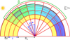 |
Fig. 1 Red-colored grid is a polar grid (α*, z) to which the radial ticks are set as the altitude corresponding to levels of pressure in the day side of the planet. The input pressure-based grid (α*, P) is also represented in the same coordinate system (colored cells from yellow to purple). |
2 2D model
The forward model used in TauREx 2D is formally described in Falco et al. (2022). Here, we provide a short presentation of the model and refer to the abovementioned paper for more information.
The model relies on the assumption that the atmosphere is symmetrical around the star-observer axis. The computation of the transmission spectrum therefore reduces to a 2D problem.
A 1D pressure profile is first defined within the assumption of a plane-parallel atmosphere, in a fashion similar to TauREx (Al-Refaie et al. 2021). The temperature is then defined in a 2D coordinate system (α*, P) of which one dimension is angular and the second is pressure-based. This coordinate system is shown by the underlying (black) grid in Fig. 1. The temperature, defined by Eq. (1), follows a linear transition between −β/2 and β/2 as proposed in Caldas et al. (2019); Wardenier et al. (2022):
 (1)
(1)
It relies on three temperature variables (Tday, Tnight, and Tdeep), an angle parameter (β), and a pressure level defining the upper limit of an isothermal annulus (Piso). This parametrization, although simplistic, is based on GCM simulations (Showman et al. 2015; Parmentier et al. 2018; Tan & Komacek 2019) to capture the most salient features of the thermal structure of HJs.
The temperature is shown by the colors (yellow to purple) in Fig. 1. The data (pressure, temperature, and abundances) in the input grid (α*, P) are then interpolated in an altitude-based coordinate system (α*, z), shown by the red grid in Fig. 1. Using the new coordinate system (α*, z), rays of light crossing the atmosphere may be subdivided into a list of segments, as illustrated in Falco et al. (2022), using simple geometric formula. There is one ray per layer in the model. The length of a ray r, which crosses the ith atmospheric layer, is identified with Δℓr,i. The optical depth can then be computed for each ray r with the following:
 (2)
(2)
where Pr,i and Tr,i are the pressure and temperatures of the cell corresponding to the segment i of the ray r, kB is the Boltzmann constant, χmr,i is the volume-mixing ratio of the m-th molecule, σm,λ is the total cross section of Rayleigh scattering and molecular and continuum absorptions, and kmie.j is the cross section associated with the Mie scattering for the jth aerosol. In addition, Ngas is the number of chemical species and Ncon is the number of aerosols. We take collision-induced absorption for H2−H2 and H2−He pairs from HITRAN into account (Richard et al. 2012). Conventionally, the contribution of collision-induced absorpion (CIA) opacities is normalized to the number of H2 molecules and included in  .
.
The volume-mixing ratios for all the species can also be differentiated with a day and a night value array. In this work, we have set the number of layers to 100 and the number of angular points (or slices) to 24. These two numbers are a good compromise between precision of the model and computational speed (Falco et al. 2022). Two angular points correspond to the full day and night sides, while the rest equally subdivide the space between −β/2 and β/2, accounting for the linear transition in between.
We tested TauREx 2D retrievals using three different configurations described in Table 1. In all three configurations, the thermal structure of the atmosphere is described using the following free parameters:
β angle, the angle across the terminator line within which we computed the radiative transfer equation;
Piso, the pressure of the boundary between the lower and the upper level;
Rp, the 10 bar radius of the planet;
Tday/night/deep, the temperature in the day and night side of the planet and in the deeper isothermal region, respectively; and
Pclouds, the pressure of the upper level of the cloud deck.
The TauREx 2D retrieval code is configured to have a deep atmospheric region where the molecular abundances and the temperature remain constant: at pressures higher than Piso, the temperature is equal Tdeep and the volume-mixing ratio of each molecule has a constant value. In the upper part of the atmosphere, where P < Piso, the temperature is different between the day side (Tday) and the night side (Tnight).
For the chemistry, we can use two different schemes:
Constant (or “free”) chemistry mode, where volume-mixing ratios are constant within each column (a) for P < Piso. In this mode, TauREx 2D can fit the abundances on each hemisphere independently; this implies three free parameters per molecule ([mol]side1, [mol]side2, and [mol]deep);
Thermal dissociation mode, where we assume local equilibrium chemistry. In this mode, the free parameters are the deep abundances of each molecule ([mol]), which are considered uniform over the planet, but we recomputed the local abundances as a function of the local pressure and temperature following Parmentier et al. (2018). In the regime we consider, these changes in abundances are mainly driven by thermal dissociation.
The thermal dissociation module we use in this work follows the parametrization of Parmentier et al. (2018), which uses a modified version of the NASA CEA Gibbs minimization code (Gordon et al. 1984) in a grid of models to investigate gas and condensate equilibrium chemistry in differrent atmospheric conditions in substellar objects (Moses et al. 2013; Kataria et al. 2015; Skemer et al. 2016; Wakeford et al. 2017; Burningham et al. 2017; Marley et al. 2017). While the constant chemistry mode could seem better as it offers more flexibility, we show that its higher number of parameters creates more degeneracies than the other parametrization (see Sect. 4) so that the thermal dissociation mode is our default except when stated otherwise. In the tests we show in the next sections, we assumed constant 30 ppm error bars in the considered wavelength range 0.5−10 µm. The assumed error was kept throughout the whole spectral range with a normal distribution (Greene et al. 2016). This value was used as a noise floor in Pluriel et al. (2022, 2020) and it is a good representation of the average noise computed using the estimated mean number of photoelectrons in Cowan et al. (2015) for a WASP-121b-like star at 270 pc during a single transit. This wavelength range will be covered using MIRI and NIRSpec instruments on board of the JWST space telescope (Gardner et al. 2006).
Input parameters for the three atmosphere configurations.
3 Test and validation
In all of the test cases, we assume the same planetary and stellar parameters as of the system WASP-121, whose values are specified in Table 2. TauREx 2D works within the same Bayesian framework as the 1D TauREx retrieval code (Al-Refaie et al. 2021). The atmospheric retrieval, which uses a 2D forward model, is more computationally intensive than the one calculated with a 1D forward model due to its additional number of parameters and geometrical dimensions.
Before focusing on a realistic test case computed using SPARC/MITgcm (Showman et al. 2009), it is fundamental to test the reliability of the TauREx 2D code on some synthetic spectra generated by itself. We decided to test the code using the three cases described in Table 1. For these tests, the input spectra have been generated by the TauREx 2D forward model itself. The three cases represent three different scenarios with different pressure-temperature (PT) profiles and then H2O mixing ratio profiles as shown in Fig. 2. All the simulated spectra have been generated assuming a resolution R = λ0/Δλ = 100, where λ0 = 5.25 µm and Δλ = [0.5µm−10µm].
The retrieval tests were performed using the MultiNest algorithm (Feroz et al. 2009) with 1000 live points and uniform prior distribution between the bounds shown in Table 2. In the next three subsections, we discuss the results for the three test configurations. For the sake of conciseness, the fitted spectrum and posterior distributions are only shown for the third, most complex case. To summarize, the three tests show that TauREx 2D can perfectly retrieve itself when there is enough information in the input spectrum.
Input planetary and stellar parameters.
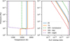 |
Fig. 2 Pressure temperature (left) and log [H2O] mixing ratio (right) profiles for the three different test cases: FI, fully isothermal; TL, two layers; and DN, day-night cases. The DN case has been split into three curves showing the profiles at the therminator, the day side, and the night side. |
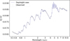 |
Fig. 3 Best-fit spectrum for the day and night convergence test. |
3.1 Fully isothermal atmosphere
A fully isothermal atmosphere represents the simplest assumption in our test set. We assumed a constant vertical as well as day and night composition with H2O and CO defined in Table 1.
The solution found is consistent with the input model. TauREx 2D found a solution which is consistent with the input parameters. TauREx found a volume-mixing ratio for log ![Mathematical equation: $\left[ {{{\rm{H}}_{\rm{2}}}{\rm{O}}} \right] = - 3.30_{ - 0.01}^{ + 0.01}$](/articles/aa/full_html/2022/11/aa43492-22/aa43492-22-eq4.png) for water and log
for water and log ![Mathematical equation: $\left[ {{\rm{CO}}} \right] = - 3.36_{ - 0.06}^{ + 0.05}$](/articles/aa/full_html/2022/11/aa43492-22/aa43492-22-eq5.png) for CO, centered around the ground truth for this case. Since we used a forward model with two vertical layers, divided at pressure Piso, TauREx found the best model where the upper layer is suppressed at the top of the atmosphere around 10−3.07 Pa and treated the rest of the atmosphere as isothermal with
for CO, centered around the ground truth for this case. Since we used a forward model with two vertical layers, divided at pressure Piso, TauREx found the best model where the upper layer is suppressed at the top of the atmosphere around 10−3.07 Pa and treated the rest of the atmosphere as isothermal with  , which is consistent with the input model.
The 2D model of TauREx is equivalent to the 1D version of TauREx in the case of isothermal atmospheres, as demonstrated in Falco et al. (2022). Therefore, this retrieval test is a confirmation of the consistency of the implementation with its 1D predecessor.
3.2 Two vertical layers atmosphere
The test case with two layers is an atmosphere where the lower layer has a temperature Tdeep = 1800 K and the upper temperature has Tupper day/night = 2600 K, but we do not have any day or night difference. We used the deep abundances defined in Table 1 and let molecules dissociate as a function of the pressure and temperature. This test is important to verify whether our model can find the input vertical structure of the atmosphere, without including day or night effects. When Tupper ≠ Tdeep, the code should recover the input Piso and two different temperatures. When Tupper = Tdeep, it should converge at the isothermal configuration.
We chose these parameters for the two-layer configuration to demonstrate how TauREx 2D can converge at the correct temperature structure, given that the composition remains the same in both hemispheres and with a temperature inversion between the lower and the upper part of the atmosphere. For such a test, we put the pressure threshold Piso between the two layers at 1 mbar, which corresponds to the range of pressures probed in such hot atmospheres, thus ensuring that the input spectrum should encode some information about the temperature change.
TauREx 2D found a  ,
,  ,
,  , and log
  . TauREx favors a thin upper atmosphere and fits the lower layer with an isothermal at ~2600 K, which is the input upper temperature. This means that we managed to probe only the upper layer of the atmosphere. The retrieved molecular abundances found are compatible with the input values log
 ![Mathematical equation: $\left[ {{{\rm{H}}_{\rm{2}}}{\rm{O}}} \right] = - 3.33_{ - 0.01}^{ + 0.01}$](/articles/aa/full_html/2022/11/aa43492-22/aa43492-22-eq11.png) for water and log
for water and log ![Mathematical equation: $\left[ {{\rm{CO}}} \right] = - 3.34_{ - 0.04}^{ + 0.05}$](/articles/aa/full_html/2022/11/aa43492-22/aa43492-22-eq12.png) .
.
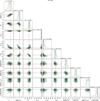 |
Fig. 4 Posterior distribution for the day and night case. The input spectrum refers to a hot atmosphere with three different equilibrium temperatures: lower temperatures, upper day, and upper night. As in the previous models, H2O and H2 can dissociate as a function of P (Pa) and T (K). The red lines represent the input values to generate the input spectrum. |
3.3 Day and night atmosphere
With this complex test, we explored the most complex atmospheric configuration in our test cases. Indeed, the input spectrum was generated assuming an isothermal inner annulus at Tdeep = 2500 K, a day-side temperature Tday = 3300 K, and a night side of Tnight = 500 K with a β angle of 20° (see Table for the exact setting). The day and night thermal difference is realistic according to GCM models of this type of planet (e.g., WASP-121b) and, within this scenario, the β parameter can give us a hint as to the 3D structure of the planet, since within this angle we probe both the day side and the night side around the terminator line. Based on these GCM equatorial temperature maps, the atmosphere can be approximated to an isothermal day and night sides, with a sharp transition region between the two sides (represented by the β parameter), and a isothermal ring under a certain pressure. Within this scenario, the parameter can also give us a hint as to the 3D structure of the planet, since within this angle we probe both the day side and the night side around the terminator line. In Fig. 3, we show the best-fit model for this last test case.
In Fig. 4, we can see how TauREx finds a unique solution around the ground truth represented by the vertical red lines. With this final convergence test, we can see the reliability of TauREx 2D with handling spectra from bidimensional models. We let the Piso and β as free parameters and, we gave TauREx the possibility to look for the best spectrum.
The β parameter retrieved with TauREx 2D, in particular, would give us valuable information to model 3D effects of an exoplanetary atmospheres. We see in Fig. 4 that TauREx found the parameters of the input spectrum.
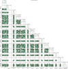 |
Fig. 5 Posterior distribution for a particular case of the fully isothermal atmosphere with different water abundances in the day (log[H2O]day = −5.3) and the night side (log[H2O]night = −4.3). |
4 Intrinsic degeneracies in transmission spectra: how to recover independently the compositions of the day and night sides
By construction, the transmission spectrum of a planet only depends on the total optical depth of the atmosphere along the various rays of light passing through the limbs (see Eq. (2)). Therefore, it can be seen right away that the transmission spectrum of a planet would remain unaffected if we took a mirror image of the planet, moving the day side from the star.
This intrinsic symmetry of the problem tells us that, technically, a retrieval algorithm cannot determine the conditions on the day and night sides. At best, it can infer the presence of different conditions on both hemispheres and we have to use our physical insight to decipher what conditions correspond to what side, for example saying that the hottest hemisphere is probably the dayside one. This is why we used Tside1 and Tside2 as independent parameters in our retrievals.
However, the fact that we measured only the total optical depth creates another degeneracy: to first order, only the total column density of a species along the ray matters. To take an extreme example, if we had a completely isothermal planet with two hemispheres with different chemical compositions, the effect of a trace molecule (mol) on the spectrum would be unaffected as long as
![Mathematical equation: ${\left[ {{\rm{mol}}} \right]_{{\rm{day}}}} + {\left[ {{\rm{mol}}} \right]_{{\rm{night}}}} = {\rm{cst}}{\rm{.}}$](/articles/aa/full_html/2022/11/aa43492-22/aa43492-22-eq13.png) (3)
(3)
A homogeneous atmosphere would have the same signature as an atmosphere where all the molecules would be in a single hemisphere.
To check the performance of TauREx 2D with a fully isothermal atmosphere and a compositional difference between the day side and the night side, we simulated an input synthetic spectrum as in the fully isothermal test case, with the difference that the water abundance changes from the day (log[H2O]day = −4.3) to the night side (log[H2O]night = −3.3). As shown in the posterior distributions (Fig. 5), TauREx 2D favors the solution in which the upper layer is flattened toward the upper edge of the planetary atmosphere, in a small annulus with a pressure lower than ![Mathematical equation: $\log \left[ P \right]\left( {{\rm{Pa}}} \right) = - 2.81_{ - 0.80}^{ + 1.17}$](/articles/aa/full_html/2022/11/aa43492-22/aa43492-22-eq14.png) , and it fits an isothermal atmosphere using only the lower layer. The input temperature is found within two sigma and the lower water abundance
, and it fits an isothermal atmosphere using only the lower layer. The input temperature is found within two sigma and the lower water abundance ![Mathematical equation: $\log {\left[ {{{\rm{H}}_{\rm{2}}}{\rm{O}}} \right]_{{\rm{deep}}}} = - 3.53_{ - 0.05}^{ + 0.04}$](/articles/aa/full_html/2022/11/aa43492-22/aa43492-22-eq15.png) is within one sigma from the arithmetic average between the input abundances log[H2O]deep,input = −3.56.
is within one sigma from the arithmetic average between the input abundances log[H2O]deep,input = −3.56.
Of course, having different temperatures on both sides formally breaks this degeneracy because of the scale height effect as well as the temperature dependence of the molecular opacities (MacDonald & Lewis 2022). But the question remains whether there is enough information in a transmission spectrum to retrieve the composition of both sides independently.
To test this, we performed another retrieval on the “day and night” input spectrum used in Sect. 3.3, using TauREx 2D’s ability to model the planet with independent compositions for the day and night sides as described in Sect. 2 (“free” mode). The posterior distributions for this retrieval are shown in Fig. 6, and the best-fit spectra found by the two models (along with the residuals) are shown in Fig. 7.
As can be seen in the bottom panel of Fig. 7, the residuals are well below the 30 ppm noise floor used as uncertainty in these retrievals. The two approaches thus give an acceptable fit. However, it can be seen in Fig. 6 that the posterior distributions of the “free” retrieval show a lot of cross correlations between several parameters. In particular, as can be expected from the argument above, when the CO or H2O abundances are high on one side, they can be very low on the other. This model also seems to miss the temperature dichotomy between the two hemispheres of the planet.
To see whether these two forward models can be statistically differentiated, we introduced the (logarithmic) Bayes factor:
 (4)
(4)
where Ed and Ef are Bayesian evidence for the retrievals with dissociation (d) and free (f) models.
Given that Bayesian evidence of the retrieval that uses thermal dissociation and coupled day and night sides is Ed = 2914, while the one related to the model that uses independent day and night sides is Ef = 2908, it follows that the Bayes factor is ~6, giving a slight yet significant advantage to the coupled model. In this case, it seems that the higher number of free parameters penalizes the model with “free” composition.
This seems to show that there is not enough information in the input spectrum (at least with the level of uncertainty expected for a JWST-like observation) to retrieve the composition of both sides of the planet simultaneously and independently. Going further, the results even imply that the information on the temperature dichotomy in a transmission spectrum mainly comes from the link between temperature and composition in the observed atmosphere. Assuming chemical equilibrium brings a considerable amount of prior knowledge on the atmosphere. If this link seems robust in UHJs where molecular dissociation is fast enough to happen close to chemical equilibrium, it should be revisited for cooler atmospheres. For this reason, the ability to retrieve the temperature dichotomy on cooler planets might be greatly reduced compared to what is shown in Lacy & Burrows (2020), where they assume chemical equilibrium to hold down to day-side temperatures near 1200 K. This issue should be thoroughly investigated.
For all of these reasons, in the following, we continue to use the model assuming thermal dissociation at chemical equilibrium as it possesses fewer free parameters and results in less correlated posterior distributions between the parameters. We should, however, keep in mind that this assumption should be revisited when modeling cooler atmospheres.
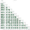 |
Fig. 6 Posterior distribution for a retrieval test made using the same “day and night” input spectrum as in Fig. 4, but retrieved using a forward atmospheric model with independent compositions for the day and night sides. One can see the strong cross correlations between the abundances of a given molecule on the day and night sides. |
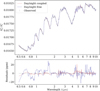 |
Fig. 7 Spectral comparison between the two day and night retrieval cases. We can see that both the coupled model (the model that considers thermal dissociation in the atmosphere) and the “free” model (which is the one that considers a constant chemistry, but independent on both sides of the planets) lead to a consistent spectrum. |
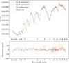 |
Fig. 8 Best-fit model for an atmosphere without optical absorbers. The TauREx 2D retrieval code found two possible solutions for this case. The comparison with the retrieval made with a 1D isothermal forward model shows that TauREx 2D leads to a better interpretation of the atmosphere. |
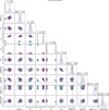 |
Fig. 9 Posterior distribution for the case where we used a WASP-121b GCM’s synthetic atmosphere as input and employing only H2O and CO a trace gases. The red lines correspond to the input deep abundances from the GCM model atmosphere. |
5 A GCM retrieval
After validating the TauREx 2D retrieval code on some self-generated spectra, we tested its abilities on a more realistic atmosphere, generated by the SPARC/MIT GCM and described in detail in Parmentier et al. (2018). We simulated the transmission spectra using 30ppm photon noise as described in Sect. 2. We used the temperature map obtained by the GCM simulation and computed the radiative transfer equation through an HJ atmosphere with Pytmosph3R 2.0 (Falco et al. 2022). The representative planet for this test is a WASP-121 b model, where molecular species can thermally dissociate as a function of the pressure and temperature. In this model, we included TiO and VO in the atmosphere as they have been detected on WASP-121 b by Evans et al. (2018). These molecules are optical absorbers that heat the day side of the planet and create a strong thermal inversion (Fortney et al. 2008; Parmentier et al. 2015, 2018). Other molecules, ions, and metals (such as Iron detected in the UHJ WASP-76 b by Ehrenreich et al. (2020)) also significantly contribute to thermal inversion in UHJs, as pointed out by Lothringer et al. (2018). Based on this GCM model of WASP-121 b, we simulated two spectra from two different atmospheric configurations to test its impact on the retrieval analysis:
A solar metallicity atmosphere with H2O and CO as trace gases; and
A solar metallicity atmosphere with H2O, CO, TiO, and VO as trace gases.
The presence of TiO and VO does indeed cover some fundamental wavelengths where Rayleigh scattering otherwise dominates. In the absence of clouds, this wavelength range allows the model to calibrate the pressure in the atmosphere and thus to have better absolute abundances. We thus want to test whether hiding these regions leads to additional biases on the retrieved parameters.
A crucial parameter related to the three-dimensionality of the planet is the β parameter. The β angle is a 2D parameter and therefore its equivalence for a 3D GCM simulation is hard to define. For the following input spectra, the best approximation we can make is  degrees based on the GCM equatorial temperature map, indicating a very sharp transition between the day and the night sides.
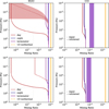 |
Fig. 10 Mixing ratio for H2O and CO for the GCM case without optical absorbers. The dashed lines are the retrieved values, while the continuous lines represent the input value. The results from the ID isothermal retrieval are in yellow. For this retrieval, the terminator and the night mixing ratios converged at the same values. |
5.1 Atmosphere without optical absorbers
We started analyzing an atmosphere without the presence of optical absorbers (e.g., molecules such as TiO and VO). The retrieval performed by TauREx 2D converged to the best-fit solution shown in Fig. 8. In this test we can also see a degenerate solution converging at two different β angles and temperatures for the two sides of the planet.
The two solutions found by TauREx have different physical properties and the best-fit parameters are shown in Fig. 9. TauREx 2D managed to converge around a realistic solution which is compatible with the ground truth, that is the parameters used to generate the input spectrum. Indeed, as shown by the red line in Fig. 9, the deep atmosphere trace gas parameter volume-mixing ratios are compatible with the ground truth of the input model within 1σ error bars for both solutions. In addition, the temperatures obtained in both solutions realistically reflect the ones of WASP-121b. This 2D model is more realistic and accurate than a simpler ID model since it is able to catch day-night differences that, as shown in Pluriel et al. (2020), are crucial in HJs such as WASP-121b.
We find  and
and  for the β angle for the first and second solution, respectively, whose measures are correlated with the temperature values found in the two sides, that is
  and
and  for the first solution and
  and
and  for the second solution. Interestingly, both solutions give the same pressure level and the same temperature for the deep layer (Piso ~ 10 Pa and Tdeep ~ 1780 K). This means that the retrieval can probe approximately up to that atmospheric region, after which we approximated the atmosphere with an isothermal annulus of Tdeep ~ 1780 K. The β parameter gives us a hint as to the 3D structure of the planet since it spans above the day side and the night side, and a dramatic change in this parameter can lead to a dramatic change in the retrieved temperature on both sides of the planet. In both solutions, the transition between the day and the night side retrieved is sharp since it is less than 12°.
The mixing ratio retrieved by the 2D model and the PT profile approximates the input profiles better than the ID model, as shown in Figs. 10 and 11. Both solutions from the 2D retrieval are closer to the input mixing ratio profiles than the solution of the ID isothermal model. In particular, TauREx 2D found the correct abundance of water in the night side and the correct value of CO within a 2σ error.
To evaluate the contribution of a 2D retrieval model, we compared the solution given by a 2D model with the one provided with a ID simple model, where we also took molecular dissociation along the vertical dimension of the atmosphere into account. From Pluriel et al. (2022), we saw how ID models cannot interpret the input spectrum of 2D models. To quantify how compares the 2D model is to the ID one, we can calculate the logarithmic Bayes factor expressed in Eq. (4).
The resulting logarithmic Bayes factor for the 2D model compared to the ID one is ℬ = +89.2, which favors the solution of the 2D retrieval over the ID one with a σ significance higher than 5σ (Trotta 2008). For this test case, without molecules hiding the spectral part with a significant contribution from the Rayleigh scattering, the 2D retrieval converges at the input spectrum compatibly with the input parameters of the synthetic spectrum. An important goal of this result is to have managed to unravel the biases observed in Pluriel et al. (2020) in the molecular abundances of the atmospheric gases. In addition, the parametrization of our 2D retrieval model develops a thermal structure of the atmosphere which is compatible with 3D GCM models.
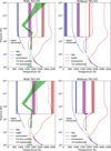 |
Fig. 11 PT profile retrieved compared to the input PT profile. In both scenarios, with and without TiO and VO, the PT profile with temperature inversion has been used. The night, terminator, and day-side PT profile of both the input (continuous line) and the retrieved models (dashed lines) are in blue, purple, and red, respectively. In the upper and lower part, we show the first and the second solution from the 2D retrievals, respectively. The solutions from a ID retrieval using the four PT point profile (only for the GCM case with optical absorbers) and the isothermal PT profile are in green and yellow, respectively. |
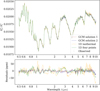 |
Fig. 12 Best-fit model for a GCM’s synthetic atmosphere with TiO and VO as optical absorbers. TauREx 2D retrieval code found two possible solutions for this case (the red and the blue one for the solution with β = 4.3 and β = 10.0 degrees, respectively). The solutions from the ID retrieval using an isothermal profile and a four PT point profile are shown in yellow and green, respectively. |
5.2 Atmosphere with optical absorbers
After studying the case of an atmosphere without TiO and VO as optical absorbers, we wanted to measure how the solution of a spectral retrieval in the presence of optical absorbers is impacted. Given the degeneracy of the TiO and VO and the Rayleigh scattering at short wavelengths and, depending on the spectral resolution and wavelength range of the data set, it could be common to not be able to disentangle the contribution of the Rayleigh scattering from the one of the optical absorbers correctly. The suggested Bayesian model has 11 free parameters and runs in ~ 20 days on 20 CPU cores using 1000 live points. The best-fit models found by TauREx 2D are shown in Fig. 12.
The results are similar to the previous retrieval: (i) TauREx 2D finds two different solutions that provide the same atmospheric spectrum (ii) converging around two beta angles,  and
and  , (iii) with the expected deep abundance of each molecule getting considered. As we increase the degrees of freedom of the model (in our case, we have an additional spatial dimension compared to the ID atmospheric model), the degeneracy of the solution could be a normal consequence that we need to handle. The β0 angle found in this simulation is ~3 degrees higher than the β0 solution found in the retrieval without optical absorbers. In the presence of TiO and VO, we can probe a more extensive part of the day side in the high atmosphere and, then, TauREx finds a greater retrieved β angle for this latter case.
From Fig. 12 it is difficult to understand the contribution of the Rayleigh scattering under the TiO and VO absorption bands. In that spectral region, the H2−H2 CIA also provides a continuum contribution, with a peak at around 2.2 µm. Compared to the case without optical absorption, we have a precision decrease from 0.02 dex to 0.10 dex, which is related to the loss of a clear Rayleigh slope signal.
In Fig. 13, we show the retrieved thermal structure for this simulation, together with the equatorial cut view of the model. In Fig. 14, we can see that the 2D retrieval managed to converge around the input mixing ratios for the four molecules. The temperatures retrieved are  K and
K and  K for the first solution,
  K and
K and  K for the second solution, and Tdeep ~ 1800 K for both solutions.
Also, in this test, the volume-mixing ratio retrieved by the 2D model and the PT profile approximates the input profiles better than the 1D retrieval, as shown in Figs. 11 and 15. TauREx 2D found two solutions, approximating the input day and night temperatures and estimating the deep atmosphere around its average temperature (Fig. 11). Moreover, TauREx 2D found a chemical distribution of elements closer to the input distribution than the one found with the 1D retrievals (Fig. 15).
The crucial result of this test is that TauREx 2D manages to retrieve the expected deep abundance of each molecule with a very good agreement to fit the input data. TauREx 2D correctly separates the contribution of the Rayleigh scattering from the one of the optical absorbers, also unraveling the biases explained in Pluriel et al. (2020). Also, in this case, a comparison with an equivalent 1D retrieval leads to a Bayes factor ℬ = +47.9 in favor of the 2D retrieval.
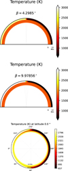 |
Fig. 13 Top and middle: temperature model for the two different solutions found in the GCM retrieval with optical absorbers. For visual reasons, the size of the atmosphere has been doubled. The temperature structure in the top represents the one of the first solution, the green one in Fig. 9. In the middle, there is the thermal structure corresponding to the second, violet solution of Fig. 14. Bottom: temperature map (equatorial cut) of WASP-121 b GCM simulation. |
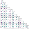 |
Fig. 14 Best-fit model for an atmosphere with TiO and VO as optical absorbers. The TauREx 2D retrieval code found two possible solutions for this case. The red lines correspond to the known deep input abundances in the GCM model. |
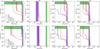 |
Fig. 15 Mixing ratio for H2O, CO, TiO, and VO in the GCM test retrieval. The dashed lines are the values retrieved by TauREx, while the continuous lines represent the input value. The results from the 1D isothermal retrieval are in yellow and we show the solution found using a four-point PT profile forward model in green. For this retrieval, the terminator and the night-mixing ratios converged at the same values. |
Comparison of models.
6 Comparison with a more complex 1D model retrieval
The 2D retrieval, in this case, helps us explore more on the 3D structure of the planet. We see that the two different solutions differ mainly from two possible β angles which lead to two possible values of Tday. We remark that a higher β angle results in a higher day-side temperature.
To quantify the goodness of the fit and see the advantages of a 2D retrieval over the “classic” 1D one, we fit the same input spectrum with a 1D model and calculated the Bayes factor between the two best-fit models. We tested the 1D model twice, assuming two different pressure-temperature profiles: one isothermal atmosphere and one four-point PT profile atmosphere.
In Table 3, we can find a resume of all the comparisons made between the 2D retrieval, including TiO and VO and the 1D retrievals. Together with the Bayesian evidence, we also provide the reduced  of each best model which is defined as follows:
 (5)
(5)
where O and C are the observed and the computed spectral points, respectively, σ is the uncertainty, p is the number of parameters in the model, and N is the total number of measurements. As described in Table 3, the 2D models approximate the input spectrum better, returning the lowest  with respect with the 1D retrievals.
In Fig. 12, we can see that the four PT points retrieval leads to a better retrieval than the one done using an isothermal atmosphere. The logarithmic Bayes factor ℬ = log E4pt − log Eiso = 33 confirms that the four-points retrieval is statistically better than the isothermal retrieval with a σ significance higher than 5σ.
A comparison between the 2D and the four-points retrieval leads to a logarithmic Bayes factor of ℬ = log E2D − log E4pt = 14 and, thus, the 2D retrieval is also better than the four-points retrieval with a σ significance higher than 5σ. The reduced  of the four-points retrieval tells us that the atmospheric model found is compatible with the input spectrum.
All the molecular abundances appear to be overestimated and, thus, biased compared to the input parameters used to generate the input spectrum.
The calculation of the Bayes factor allowed us to quantify the goodness of the 2D retrieval compared to the 1D one. Indeed, if we consider only the reduced  of the fit, we see that the single models are compatible with the input spectra with a high significance. However, it is impossible to get rid of the parameter biases when using the 1D model. The key point of the calculation of the logarithmic Bayes factor is to highlight the fundamental differences of the two model and the limits given by their geometry. With 30ppm error bars, it is indeed possible to reveal and explain some spectral features by introducing an additional geometric dimension on the atmospheric model.
Indeed, even though the 1D retrieval converges toward a statistically significant atmospheric model, the parameters found can differ from the ground truth by several orders of magnitude. In Fig. 16, as an example, we show the posterior distributions for a retrieval of the GCM input spectrum with optical absorbers, using a 1D atmospheric model and four temperature-pressure points. The best model fits the input spectrum very well, but the retrieved amount of atmospheric trace gases differs from the ground truth by up to two orders of magnitude.
We see that the logarithmic Bayes factor defined in Eq. (4), which expresses the difference of the 2D model compared with the 1D one, is ℬ = +47.9. This favors the solution of the bidimensional model with a σ significance higher than 5σ. Also, in this case, the 2D model leads to a statistically better fit than the 1D model. The statistical significance of the 2D model is higher than that of the 1D model. In addition, it is less affected by the parameter biases since it approximates the 3D geometry of the input model better.
The comparison with the 1D retrieval emphasizes the importance of running more-than-one dimensions retrieval models when using 30 ppm noise input spectra. In the era of the JWST, ARIEL, and Twinkle space missions it will be of fundamental importance to use better models which rely on more complex geometrical assumptions than the plane parallel atmospheres.
 |
Fig. 16 Posterior distributions related to the four-points retrieval. Confirming the parameter biases found by Pluriel et al. (2022). |
7 Conclusion
More-than-1D retrievals will be crucial to interpret the input spectral observation of new generation instruments better. Even though the approximation of a plane-parallel atmosphere can lead to a statistically acceptable fit, it inevitably leads to parameter biases that can be very far away from the reality (Pluriel et al. 2020, 2022). This is especially true for HJs and UHJs, where the great dichotomy between the day and the night side of the planet may lead to a misinterpretation of the input observations, without an accurate model.
We developed a 2D version of TauREx, which demonstrates that a 2D forward model is a good compromise between model accuracy and computational requirements. This model can solve the issues of the parameter biases induced by a 1D model which is essential in the context of future mission such as JWST, Twinkle, or Ariel. Thanks to TauREx 2D, we are able to determine the abundances of the species with much higher confidence than with 1D retrieval models.
We have shown how the model choice could be crucial to retrieve the thermal structure of an exoplanetary atmosphere properly (in Sect. 4), due to the intrinsic degeneracies of a high dimensional transmission model. Finally, in Sect. 6 we demonstrate how a 2D retrieval with an isothermal atmosphere returns a statistically more significant solution than a 1D retrieval using a more complex four-point pressure-temperature profile.
Acknowledgements
This project has received funding from the European Research Council (ERC) under the European Union’s Horizon 2020 research and innovation programme (grant agreement no. 679030/WHIPLASH). T.Zi acknowledges the funding support from Italian Space Agency (ASI) regulated by ‘Accordo ASI-INAF no. 2013-016-R.0 del 9 luglio 2013 e integrazione del 9 luglio 2015 CHEOPS Fasi A/B/C’.
References
- Al-Refaie, A. F., Changeât, Q., Waldmann, I. P., & Tinetti, G. 2021, ApJ, 917, 37 [NASA ADS] [CrossRef] [Google Scholar]
- Baeyens, R., Decin, L., Carone, L., et al. 2021, MNRAS, 505, 5603 [NASA ADS] [CrossRef] [Google Scholar]
- Barstow, J. K., Changeat, Q., Garland, R., et al. 2020, MNRAS, 493, 4884 [NASA ADS] [CrossRef] [Google Scholar]
- Beichman, C., Benneke, B., Knutson, H., et al. 2014, PASP, 126, 1134 [NASA ADS] [CrossRef] [Google Scholar]
- Brown, T. M. 2001, ApJ, 553, 1006 [NASA ADS] [CrossRef] [Google Scholar]
- Burningham, B., Marley, M. S., Line, M. R., et al. 2017, MNRAS, 470, 1177 [NASA ADS] [CrossRef] [Google Scholar]
- Caldas, A., Leconte, J., Selsis, F., et al. 2019, A&A, 623, A161 [NASA ADS] [CrossRef] [EDP Sciences] [Google Scholar]
- Changeat, Q., & Al-Refaie, A. 2020, ApJ, 898, 155 [NASA ADS] [CrossRef] [Google Scholar]
- Changeat, Q., & Edwards, B. 2021, ApJ, 907, L22 [NASA ADS] [CrossRef] [Google Scholar]
- Changeat, Q., Edwards, B., Waldmann, I. P., & Tinetti, G. 2019, ApJ, 886, 39 [NASA ADS] [CrossRef] [Google Scholar]
- Charnay, B., Meadows, V., Misra, A., Leconte, J., & Arney, G. 2015, ApJ, 813, L1 [NASA ADS] [CrossRef] [Google Scholar]
- Cowan, N. B., Greene, T., Angerhausen, D., et al. 2015, PASP, 127, 311 [NASA ADS] [CrossRef] [Google Scholar]
- Deming, D. 2010, Nature, 468, 636 [NASA ADS] [CrossRef] [Google Scholar]
- Drummond, B., Tremblin, P., Baraffe, I., et al. 2016, A&A, 594, A69 [NASA ADS] [CrossRef] [EDP Sciences] [Google Scholar]
- Ehrenreich, D., Lovis, C., Allart, R., et al. 2020, Nature, 580, 597 [Google Scholar]
- Espinoza, N., & Jones, K. 2021, AJ, 162, 165 [NASA ADS] [CrossRef] [Google Scholar]
- Evans, T. M., Sing, D. K., Goyal, J. M., et al. 2018, AJ, 156, 283 [NASA ADS] [CrossRef] [Google Scholar]
- Falco, A., Zingales, T., Pluriel, W., & Leconte, J. 2022, A&A 658 A41 [NASA ADS] [CrossRef] [EDP Sciences] [Google Scholar]
- Feng, Y. K., Line, M. R., Fortney, J. J., et al. 2016, ApJ, 829, 52 [NASA ADS] [CrossRef] [Google Scholar]
- Feng, Y. K., Line, M. R., & Fortney, J. J. 2020, AJ, 160, 137 [NASA ADS] [CrossRef] [Google Scholar]
- Feroz, F., Hobson, M. P., & Bridges, M. 2009, MNRAS, 398, 1601 [NASA ADS] [CrossRef] [Google Scholar]
- Fortney, J. J., Lodders, K., Marley, M. S., & Freedman, R. S. 2008, ApJ, 678, 1419 [CrossRef] [Google Scholar]
- Fortney, J. J., Shabram, M., Showman, A. P., et al. 2010, ApJ, 709, 1396 [NASA ADS] [CrossRef] [Google Scholar]
- Gandhi, S., & Madhusudhan, N. 2018, MNRAS, 474, 271 [Google Scholar]
- Gardner, J. P., Mather, J. C., Clampin, M., et al. 2006, Space Sci. Rev., 123, 485 [Google Scholar]
- Gordon, S., McBride, B., & Zeleznik, F. J. 1984, Computer Program for Calculation of Complex Chemical Equilibrium Compositions and Applications. Supplement 1: Transport Properties [Google Scholar]
- Greene, T. P., Line, M. R., Montero, C., et al. 2016, ApJ, 817, 17 [NASA ADS] [CrossRef] [Google Scholar]
- Heng, K., Frierson, D. M. W., & Phillipps, P. J. 2011, MNRAS, 418, 2669 [NASA ADS] [CrossRef] [Google Scholar]
- Irwin, P. G. J., Teanby, N. A., de Kok, R., et al. 2008, J. Quant. Spec. Radiat. Transf., 109, 1136 [NASA ADS] [CrossRef] [Google Scholar]
- Kataria, T., Showman, A. P., Fortney, J. J., et al. 2015, ApJ, 801, 86 [NASA ADS] [CrossRef] [Google Scholar]
- Kataria, T., Sing, D. K., Lewis, N. K., et al. 2016, ApJ, 821, 9 [NASA ADS] [CrossRef] [Google Scholar]
- Kreidberg, L. 2018, in Handbook of Exoplanets, eds. H. J. Deeg, & J. A. Belmonte, 100 [Google Scholar]
- Lacy, B. I., & Burrows, A. 2020, ApJ, 905, 131 [NASA ADS] [CrossRef] [Google Scholar]
- Line, M. R., & Parmentier, V. 2016, ApJ, 820, 78 [Google Scholar]
- Line, M. R., Wolf, A. S., Zhang, X., et al. 2013, ApJ, 775, 137 [NASA ADS] [CrossRef] [Google Scholar]
- Lothringer, J. D., Barman, T., & Koskinen, T. 2018, ApJ, 866, 27 [NASA ADS] [CrossRef] [Google Scholar]
- MacDonald, R. J., & Lewis, N. K. 2022, ApJ, 929, 20 [NASA ADS] [CrossRef] [Google Scholar]
- MacDonald, R. J., & Madhusudhan, N. 2017, ApJ, 850, L15 [NASA ADS] [CrossRef] [Google Scholar]
- MacDonald, R. J., Goyal, J. M., & Lewis, N. K. 2020, ApJ, 893, L43 [NASA ADS] [CrossRef] [Google Scholar]
- Madhusudhan, N., & Seager, S. 2009, ApJ, 707, 24 [NASA ADS] [CrossRef] [Google Scholar]
- Marley, M. S., Saumon, D., Fortney, J. J., et al. 2017, in American Astronomical Society Meeting Abstracts, 230, 315.07 [NASA ADS] [Google Scholar]
- Menou, K., & Rauscher, E. 2009, ApJ, 700, 887 [NASA ADS] [CrossRef] [Google Scholar]
- Mikal-Evans, T., Sing, D. K., Barstow, J. K., et al. 2022, Nat. Astron., 6, 471 [NASA ADS] [CrossRef] [Google Scholar]
- Min, M., Ormel, C. W., Chubb, K., Helling, C., & Kawashima, Y. 2020, A&A, 642, A28 [NASA ADS] [CrossRef] [EDP Sciences] [Google Scholar]
- Molaverdikhani, K., Henning, T., & Mollière, P. 2019, ApJ, 883, 194 [Google Scholar]
- Mollière, P., Wardenier, J. P., van Boekel, R., et al. 2019, A&A, 627, A67 [Google Scholar]
- Moses, J. I., Line, M. R., Visscher, C., et al. 2013, ApJ, 777, 34 [Google Scholar]
- Nixon, M. C., & Madhusudhan, N. 2022, ApJ 935 73 [NASA ADS] [CrossRef] [Google Scholar]
- Parmentier, V., Guillot, T., Fortney, J. J., & Marley, M. S. 2015, A&A, 574, A35 [NASA ADS] [CrossRef] [EDP Sciences] [Google Scholar]
- Parmentier, V., Fortney, J. J., Showman, A. P., Morley, C., & Marley, M. S. 2016, ApJ, 828, 22 [Google Scholar]
- Parmentier, V., Line, M. R., Bean, J. L., et al. 2018, A&A, 617, A110 [NASA ADS] [CrossRef] [EDP Sciences] [Google Scholar]
- Pluriel, W., Zingales, T., Leconte, J., & Parmentier, V. 2020, A&A, 636, A66 [EDP Sciences] [Google Scholar]
- Pluriel, W., Leconte, J., Parmentier, V., et al. 2022, A&A, 658, A42 [NASA ADS] [CrossRef] [EDP Sciences] [Google Scholar]
- Richard, C., Gordon, I. E., Rothman, L. S., et al. 2012, JQSRT, 113, 1276 [NASA ADS] [CrossRef] [Google Scholar]
- Rodgers, C. D. 2000, Inverse Methods for Atmospheric Sounding: Theory and Practice [Google Scholar]
- Showman, A. P., & Guillot, T. 2002, A&A, 385, 166 [NASA ADS] [CrossRef] [EDP Sciences] [Google Scholar]
- Showman, A. P., Cooper, C. S., Fortney, J. J., & Marley, M. S. 2008, ApJ, 682, 559 [NASA ADS] [CrossRef] [Google Scholar]
- Showman, A. P., Fortney, J. J., Lian, Y., et al. 2009, ApJ, 699, 564 [NASA ADS] [CrossRef] [Google Scholar]
- Showman, A. P., Lewis, N. K., & Fortney, J. J. 2015, ApJ, 801, 95 [NASA ADS] [CrossRef] [Google Scholar]
- Skemer, A. J., Morley, C. V., Zimmerman, N. T., et al. 2016, ApJ, 817, 166 [NASA ADS] [CrossRef] [Google Scholar]
- Tan, X., & Komacek, T. D. 2019, ApJ, 886, 26 [Google Scholar]
- Taylor, J., Parmentier, V., Irwin, P. G. J., et al. 2020, MNRAS, 493, 4342 [NASA ADS] [CrossRef] [Google Scholar]
- Tessenyi, M., Savini, G., Tinetti, G., et al. 2016, in AAS/Division for Planetary Sciences Meeting Abstracts, 48, 123.33 [NASA ADS] [Google Scholar]
- Tinetti, G., Drossart, P., Eccleston, P., et al. 2016, in Space Telescopes and Instrumentation 2016: Optical, Infrared, and Millimeter Wave, SPIE, 9904, 658 [Google Scholar]
- Tinetti, G., Drossart, P., Eccleston, P., et al. 2018, Exp. Astron., 46, 135 [NASA ADS] [CrossRef] [Google Scholar]
- Trotta, R. 2008, Contemp. Phys., 49, 71 [Google Scholar]
- Tsiaras, A., Waldmann, I. P., Zingales, T., et al. 2018, AJ, 155, 156 [NASA ADS] [CrossRef] [Google Scholar]
- Wakeford, H. R., Visscher, C., Lewis, N. K., et al. 2017, MNRAS, 464, 4247 [NASA ADS] [CrossRef] [Google Scholar]
- Wakeford, H. R., Sing, D. K., Deming, D., et al. 2018, AJ, 155, 29 [Google Scholar]
- Waldmann, I. P., Rocchetto, M., Tinetti, G., et al. 2015a, ApJ, 813, 13 [Google Scholar]
- Waldmann, I. P., Tinetti, G., Rocchetto, M., et al. 2015b, ApJ, 802, 107 [CrossRef] [Google Scholar]
- Wardenier, J. P., Parmentier, V., & Lee, E. K. H. 2022, MNRAS, 510, 620 [Google Scholar]
- Welbanks, L., & Madhusudhan, N. 2022, ApJ, 933, 79 [NASA ADS] [CrossRef] [Google Scholar]
- Welbanks, L., Madhusudhan, N., Allard, N. F., et al. 2019, ApJ, 887, L20 [NASA ADS] [CrossRef] [Google Scholar]
- Wordsworth, R. D., Forget, F., Selsis, F., et al. 2011, ApJ, 733, L48 [Google Scholar]
- Zhang, M., Chachan, Y., Kempton, E. M. R., & Knutson, H. A. 2019, PASP, 131, 034501 [Google Scholar]
All Tables
All Figures
|
Fig. 1 Red-colored grid is a polar grid (α*, z) to which the radial ticks are set as the altitude corresponding to levels of pressure in the day side of the planet. The input pressure-based grid (α*, P) is also represented in the same coordinate system (colored cells from yellow to purple). |
| In the text | |
|
Fig. 2 Pressure temperature (left) and log [H2O] mixing ratio (right) profiles for the three different test cases: FI, fully isothermal; TL, two layers; and DN, day-night cases. The DN case has been split into three curves showing the profiles at the therminator, the day side, and the night side. |
| In the text | |
|
Fig. 3 Best-fit spectrum for the day and night convergence test. |
| In the text | |
|
Fig. 4 Posterior distribution for the day and night case. The input spectrum refers to a hot atmosphere with three different equilibrium temperatures: lower temperatures, upper day, and upper night. As in the previous models, H2O and H2 can dissociate as a function of P (Pa) and T (K). The red lines represent the input values to generate the input spectrum. |
| In the text | |
|
Fig. 5 Posterior distribution for a particular case of the fully isothermal atmosphere with different water abundances in the day (log[H2O]day = −5.3) and the night side (log[H2O]night = −4.3). |
| In the text | |
|
Fig. 6 Posterior distribution for a retrieval test made using the same “day and night” input spectrum as in Fig. 4, but retrieved using a forward atmospheric model with independent compositions for the day and night sides. One can see the strong cross correlations between the abundances of a given molecule on the day and night sides. |
| In the text | |
|
Fig. 7 Spectral comparison between the two day and night retrieval cases. We can see that both the coupled model (the model that considers thermal dissociation in the atmosphere) and the “free” model (which is the one that considers a constant chemistry, but independent on both sides of the planets) lead to a consistent spectrum. |
| In the text | |
|
Fig. 8 Best-fit model for an atmosphere without optical absorbers. The TauREx 2D retrieval code found two possible solutions for this case. The comparison with the retrieval made with a 1D isothermal forward model shows that TauREx 2D leads to a better interpretation of the atmosphere. |
| In the text | |
|
Fig. 9 Posterior distribution for the case where we used a WASP-121b GCM’s synthetic atmosphere as input and employing only H2O and CO a trace gases. The red lines correspond to the input deep abundances from the GCM model atmosphere. |
| In the text | |
|
Fig. 10 Mixing ratio for H2O and CO for the GCM case without optical absorbers. The dashed lines are the retrieved values, while the continuous lines represent the input value. The results from the ID isothermal retrieval are in yellow. For this retrieval, the terminator and the night mixing ratios converged at the same values. |
| In the text | |
|
Fig. 11 PT profile retrieved compared to the input PT profile. In both scenarios, with and without TiO and VO, the PT profile with temperature inversion has been used. The night, terminator, and day-side PT profile of both the input (continuous line) and the retrieved models (dashed lines) are in blue, purple, and red, respectively. In the upper and lower part, we show the first and the second solution from the 2D retrievals, respectively. The solutions from a ID retrieval using the four PT point profile (only for the GCM case with optical absorbers) and the isothermal PT profile are in green and yellow, respectively. |
| In the text | |
|
Fig. 12 Best-fit model for a GCM’s synthetic atmosphere with TiO and VO as optical absorbers. TauREx 2D retrieval code found two possible solutions for this case (the red and the blue one for the solution with β = 4.3 and β = 10.0 degrees, respectively). The solutions from the ID retrieval using an isothermal profile and a four PT point profile are shown in yellow and green, respectively. |
| In the text | |
|
Fig. 13 Top and middle: temperature model for the two different solutions found in the GCM retrieval with optical absorbers. For visual reasons, the size of the atmosphere has been doubled. The temperature structure in the top represents the one of the first solution, the green one in Fig. 9. In the middle, there is the thermal structure corresponding to the second, violet solution of Fig. 14. Bottom: temperature map (equatorial cut) of WASP-121 b GCM simulation. |
| In the text | |
|
Fig. 14 Best-fit model for an atmosphere with TiO and VO as optical absorbers. The TauREx 2D retrieval code found two possible solutions for this case. The red lines correspond to the known deep input abundances in the GCM model. |
| In the text | |
|
Fig. 15 Mixing ratio for H2O, CO, TiO, and VO in the GCM test retrieval. The dashed lines are the values retrieved by TauREx, while the continuous lines represent the input value. The results from the 1D isothermal retrieval are in yellow and we show the solution found using a four-point PT profile forward model in green. For this retrieval, the terminator and the night-mixing ratios converged at the same values. |
| In the text | |
|
Fig. 16 Posterior distributions related to the four-points retrieval. Confirming the parameter biases found by Pluriel et al. (2022). |
| In the text | |
Current usage metrics show cumulative count of Article Views (full-text article views including HTML views, PDF and ePub downloads, according to the available data) and Abstracts Views on Vision4Press platform.
Data correspond to usage on the plateform after 2015. The current usage metrics is available 48-96 hours after online publication and is updated daily on week days.
Initial download of the metrics may take a while.