| Issue |
A&A
Volume 695, March 2025
|
|
|---|---|---|
| Article Number | A72 | |
| Number of page(s) | 15 | |
| Section | Extragalactic astronomy | |
| DOI | https://doi.org/10.1051/0004-6361/202349086 | |
| Published online | 07 March 2025 | |
Keplerian molecular gas disk and black hole mass of NGC 4751
1
Departamento de Astronomía, Universidad de Concepción, Barrio Universitario s/n, Concepción, Chile
2
LIRA, Observatoire de Paris, Université PSL, CNRS, Sorbonne Université, Université Paris Cité, 5 Place Jules Janssen, 92195 Meudon, France
3
Finnish Centre for Astronomy with ESO, FI-20014 University of Turku, Finland
4
Aalto University Metsähovi Radio Observatory, Metsähovintie 114, FI-02540 Kylmälä, Finland
5
Instituto de Astrofísica, Facultad de Física, Pontificia Universidad Católica de Chile, Casilla 306, Santiago 22, Chile
6
Joint ALMA Observatory, Alonso de Córdova 3107, Vitacura, 763-0355 Santiago, Chile
7
European Southern Observatory, Alonso de Córdova 3107, Vitacura, Casilla, 19001 Santiago de Chile, Chile
8
Department of Astronomy, University of Michigan, Ann Arbor, MI 48109, USA
9
Department of Astronomy, University of Texas at Austin, Austin, TX 78712-1205, USA
10
Astronomy Department, University of Maryland, College Park, MD 20742, USA
⋆ Corresponding authors; This email address is being protected from spambots. You need JavaScript enabled to view it.
, This email address is being protected from spambots. You need JavaScript enabled to view it.
Received:
22
December
2023
Accepted:
30
December
2024
Abstract
Aims. We aim to measure the mass of the supermassive black hole (SMBH) in the S0 galaxy NGC 4751 using CO J:3−2 emission from the 5″-scale nuclear rotating molecular disk.
Methods. We imaged the kpc-scale molecular gas disk in NGC 4751 at 0.″22 (∼28 pc) spatial and 28 km s−1 spectral resolution in the CO J:3−2 emission line and neighboring continuum, with the Atacama Large Millimeter Array (ALMA). We used Hubble Space Telescope (HST) imaging and stellar and ionized gas kinematics at 100 pc to kpc-scales, derived from integral field spectroscopy, to determine the galaxy morphology and the circular velocity attributed to the stellar potential. We used the Markov chain Monte Carlo (MCMC) algorithm in the KINematic Molecular Simulation (KinMS) package to obtain the model parameters that best fit the observed molecular gas kinematics in the ALMA datacube.
Results. Strong CO emission was detected over radii of ∼0.″2 to 5″, with isolated CO clumps detected out to 7″. The molecular disk kinematics is axisymmetric and rotation-dominated, with radial velocities between 400 km s−1 and 660 km s−1, a kinematic major axis position angle (PA) of 355°, and an inclination close to 78°. The intrinsic velocity dispersion is ∼16 km s−1, and there is no evidence for significant non-rotational kinematics. The kinematic center of the disk coincides with the compact nuclear 345 GHz source. The SMBH sphere of influence (SOI) is well resolved along all position angles. The (rotation) velocity curve due to the stellar potential (Vradialmax ∼ 430 km s−1) is determined by fitting the luminosity profile of NGC 4751 in an (H-band) image from the Wide Field Camera 3 (WFC3) aboard HST, and constraining the mass-to-light ratio (M/L) at this waveband using the molecular- and ionized-gas kinematics at radii ≳4″, outside the SMBH SOI. Several KinMS fits, all using a distance (D) of 26.3 Mpc, but with variations in other input quantities, resulted in SMBH masses of 3.22 − 4.33 × 10⁹ M⊙ and M/L values of 1.1−2.3 in the F160W band. In each fit, the statistical errors of these values are on the level of a few percent.
Conclusions. Based on the results of the multiple KinMS fits, we argued for and adopted a value of 3.3 × 10⁹ (D/26.3) M⊙ for the black hole mass, along with a (constant with radius) M/L of 2.28/(26.3/D)2 in the F160W band. We estimated the (one sigma) errors to be 20% in each of these. We find that the primary driver of the uncertainty (apart from distance) is the stellar potential in this dusty S0 galaxy. This CO-based mass is ∼2.4 times higher than a previous stellar-dynamics based SMBH mass measurement using the same distance. We argue that this new value is more robust given the clear and well resolved Keplerian-rotation dominated signature in the molecular disk, as well as its robust values of inclination (78°) and PA (355°), further supported by the consistency among derived values across different datasets and methods.
Key words: galaxies: kinematics and dynamics
© The Authors 2025
 Open Access article, published by EDP Sciences, under the terms of the Creative Commons Attribution License (https://creativecommons.org/licenses/by/4.0), which permits unrestricted use, distribution, and reproduction in any medium, provided the original work is properly cited.
This article is published in open access under the Subscribe to Open model. This email address is being protected from spambots. You need JavaScript enabled to view it. to support open access publication.
1. Introduction
Direct measurements of supermassive black hole (SMBH) masses are possible only when it is possible to resolve the kinematics or dynamics within the sphere of influence (SOI) of the SMBH. Specifically, the SOI is the linear or angular scale within which the SMBH potential (rather than that of the stars or dark matter in the galaxy bulge or disk) dominates the dynamics. Since this SOI is  for all galaxies, except the Milky Way and Andromeda, decades of effort have resulted in direct SMBH mass measurements for fewer than 200 galaxies (e.g., Gültekin et al. 2009, 2011; van den Bosch 2016; Saglia et al. 2016). The bulk of these measurements come from stellar dynamic or ionized gas kinematic modeling of high resolution “integral” field spectra data sets, obtained with ground-based adaptive optics (AO) systems or with the Space Telescope Imaging Spectrograph (STIS) on board the Hubble Space Telescope (HST), from maser disk kinematics, and from molecular gas kinematics obtained with the Atacama Large Millimeter Array (ALMA).
High spatial-resolution observations from, for example, ALMA, the James Webb Space Telescope, along with ground based adaptive optics integral field unit (IFU) instruments on large telescopes, can increase the number of SMBH masses measured and, more importantly, resolve systematic differences between competing methods. The sensitivity and resolution (30 mas to a few arcseconds) of ALMA has enabled an increasing number of SMBH mass measurements via the kinematics of molecular gas disks, for example: NGC 1097 (Onishi et al. 2015), NGC 1332 (Barth et al. 2016), NGC 3665 (Onishi et al. 2017), NGC 4697 (Davis et al. 2017), NGC 4429 (Davis et al. 2018; Combes et al. 2019), NGC 3258 (Boizelle et al. 2019), NGC 315 and NGC 4261 (Boizelle et al. 2021), NGC 1380, and NGC 6861 (Kabasares et al. 2022), along with several galaxies in the WISDOM sample (North et al. 2019; Ruffa et al. 2023, and references therein). The primary limitation at ALMA is the requirement of molecular gas emission sufficiently bright at high resolution. Furthermore, a reliable SMBH mass measurement requires a fully resolved rotating disk (thereby constraining the disk inclination) and a relatively high velocity resolution (to constrain non-axisymmetric and non-circular motions in the gas; e.g., streaming inflows and outflows, perturbations related to non-axisymmetric potentials, such as bars and spiral arms, and turbulence). As an example of IFUs, the 4-laser AO assisted narrow field mode (NFM) of the Multi Unit Spectroscopic Explorer (MUSE) IFU on the Very Large Telescope (VLT; Bacon et al. 2010) now allows for an HST-like spatial resolution over a 7″ × 7″ integral field of view (FOV). The limitation here is the necessity of a “natural guide star” (NGS) within a few arcseconds of the target; the galaxy nucleus itself may be used as the NGS under certain conditions.
In this work, we present a robust and accurate SMBH mass measurement in NGC 4751 (ESO 323-G029, MCG -07-27-011) using molecular gas kinematics. This galaxy was observed by ALMA as part of a sample of galaxies with the largest subtended angular SOI (project 2016.1.01135.S; P.I. Nagar). NGC 4751 is a relatively nearby (heliocentric velocity of 2094 ± 45 km s−1 in the NED database or 1946 km s−1 in the SIMBAD database) lenticular (SA0−) galaxy, with a size of 3′ × 1′ (NED). Its distance is uncertain: Tully-Fisher distance estimates imply 35 Mpc or 46.6 Mpc (Theureau et al. 2007), while the observed heliocentric velocity (and H0 = 67.8 km s−1 Mpc−1) implies distances between, for example, 25.33 Mpc (correcting only for Virgo and Great Attractor infall) and 34.95 Mpc (correcting for only the CMB velocity dipole) according to NED. In this work, to be consistent with Rusli et al. (2013), we use a distance of 26.3 Mpc, implying a linear scale of 127 pc/arcsec.
Despite its proximity and presence in the NGC catalog (Dreyer 1888), NGC 4751 is poorly studied. Gültekin et al. (2011) listed a central velocity dispersion of 349 km s−1 for NGC 4751, and assuming a distance of 23.5 Mpc, estimated a black hole mass of 1.4 × 10⁹ M⊙ via the M–σ relationship, and thus predicted the sphere of influence to be  . Rusli et al. (2013) directly measured the black hole mass in NGC 4751 by applying stellar dynamical modeling to data sets from the Spectrograph for INtegral Field Observations in the Near Infrared (SINFONI) aboard VLT (3″ × 3″ FOV, 100 mas slitlets, a
  PSF, and 60 km s−1 velocity resolution). For their assumed distance of 26.9 ± 2.9 Mpc, they obtained a black hole mass of 1.4(±0.2)×109 M⊙ and a central velocity dispersion of 361 ± 13 km s−1 (see also Saglia et al. 2016). This black hole mass estimation was independent of whether or not a DM halo was used in modeling the galaxy mass. It should be noted that Rusli et al. (2013) used an R-band image with a corresponding mass-to-light ratio (M/L) of 8.27 (Saglia et al. 2016), to derive the galaxy rotation curve.
NGC 4751 shows compact (< 3″) nuclear radio emission with flux 3 mJy at 5 GHz (Sadler et al. 1989). Its ROSAT-traced X-ray bolometric luminosity is log LX < 40.3 erg s−1 (assuming D = 24 Mpc; O’Sullivan et al. 2001). With these results, and the lack of deep optical spectroscopy of the nucleus, the presence of a low-luminosity active galactic nucleus (AGN) could not be ruled out.
This paper is organized as follows. Section 2 presents the ALMA, VLT/MUSE and HST observations and data processing. Section 3 presents the morphological and kinematic properties of the large-scale galaxy and the nuclear molecular gas disk. Section 4 presents our methods and measurements of the black hole mass. Finally, Sect. 5 presents our conclusions.
2. Observations and data processing
2.1. ALMA
NGC 4751 was observed on May 17, 2017, using 49 antennas of the ALMA 12 m array. Antenna separations ranged from 15 m to 1.1 km. The source J1321−4342 was used as a phase calibrator, and the sources J1427−4206 (used as bandpass and amplitude calibrator) and J1308−4352 (a test source) were also observed. Of the total observation time of about 50 min, 22 min of integration were obtained on NGC 4751.
All four spectral windows (spw’s) were set to “continuum” (TDM) mode in order to achieve the highest sensitivity. Two overlapping spws were centered on the expected sky frequency of the CO J:3−2 line (rest frequency 345.79599 GHz), giving a total velocity coverage of ±1500 km s−1, and the other two windows covered continuum emission and the CS J:5−4 line. We followed standard data processing procedures in the CASA package, closely following the pipeline script delivered by the ALMA staff. Line-free channels were used to image the 345 GHz continuum emission. This continuum emission was then subtracted from the uv data set before imaging the CO emission line. Final maps and datacubes were made with “natural weighting” to achieve the highest signal-to-noise ratio (S/N) at some cost to resolution, along with a pixel size of  : here, the synthesized beam (i.e., the spatial resolution) is
  ×
×  for a position angle (PA) of −59°. On the spectral axis, we used the intrinsic observed channel spacing of 13.6 km s−1, that is, a velocity resolution of ∼27 km s−1. The root mean square (rms) noise is 0.4 mJy/beam per 13.6 km s−1 channel in the datacube, and 0.05 mJy/beam in the 345 GHz continuum map.
2.2. VLT/MUSE wide-field
NGC 4751 was observed with the MUSE IFU mounted on the VLT in its wide field mode (WFM). MUSE covers a wavelength range of 4750−9350 Å with a wavelength sampling of 1.25 Å per pixel, and has a spectral resolution (R) of 3026 at 7000 Å; the WFM mode has a FOV of 1′ × 1′, and a spatial sampling of  per pixel.
The observations were made on August 13, 2015. Data were processed with the standard MUSE pipeline (v1.6.1) and the calibrated datacubes were hosted on the ESO Archive (Processed Data Science Portal). A single processed datacube was downloaded from this archive, with a total on-sky exposure time of 1800 seconds.
We used version 3.1.0. of the GIST Pipeline software (Bittner et al. 2019) to derive the stellar and ionized gas kinematics of the galaxy, as well as the stellar population properties; namely: the weighted mean age and metallicity of the best-fit stellar templates. The stellar kinematics and stellar population properties were constrained using the version of the penalized pixel fitting technique (pPXF; Cappellari & Emsellem 2004; Cappellari 2017) included in the GIST Pipeline. The technique selects a linear combination of stellar templates that best fit the observed galaxy spectrum and delivers stellar moment maps. The set of templates used is the MILES stellar template library (Vazdekis et al. 2010) covering the range 3525−7500 Å. The Voronoi binning technique (Cappellari & Copin 2003) was used to bin spaxels in order to increase the S/N of the spectra. We set a minimum continuum S/N of 70 for each bin, with the continuum S/N calculated over the wavelength range 5700−5750 Å, where no emission line is expected to be observed, and excluding spaxels with S/N values below 3. Within GIST, pPXF was run on the wavelength range 5050−6000 Å, using four moments (velocity, velocity dispersion, and the third and fourth coefficients of the Gauss-Hermite polynomials), a tenth degree additive polynomial to derive stellar kinematics, and a fourth degree multiplicative polynomial to derive stellar population properties.
The ionized gas kinematics is derived using GANDALF (Sarzi et al. 2006; Falcón-Barroso et al. 2006; Bittner et al. 2019) within the GIST Pipeline. Here, in each spectrum, a simultaneous fit to both absorption (from the preceding pPXF run) and emission lines was used to obtain the flux, velocity, and velocity dispersion maps of the emission lines, as well as an “emission-line-only” spectrum. In GANDALF, the emission lines were modeled with Gaussians and the resulting moment maps are derived from the parameters of these fitted Gaussians. GANDALF was run on a wavelength range of 4750−7535 Å to include emission lines such as Hα+[N II].
Furthermore, we created position-velocity (pv) diagrams of individual emission lines directly from the MUSE cube to compare the data with models. Here we did not use the emission-line-only spectra from GANDALF, since these were Voronoi-binned. Instead, for each spaxel, we used emission-line free regions near the relevant emission line to create a continuum subtracted cube: the continuum was fit as a straight line and subtracted from the spectrum. The pv diagrams were extracted from the datacube along linear slits with one spaxel width.
2.3. HST
In this work, we used two images from the Wide Field Camera 3 (WFC3) aboard HST to constrain the overall galaxy morphology and derive the stellar potential of NGC 4751; these data were, in turn, used to obtain the galaxy rotation curve. Both images were taken on May 11, 2020 (Proposal ID: 15909, PI: B. Boizelle). The first image was taken with the F160W filter and a total exposure time of 997 seconds. It has a FOV of about 3.5′ × 3.5′, and a spatial sampling of  per pixel. A 20″ × 30″ subpart of this image is shown in the left panel of Fig. 1. The second image was taken with the F110W filter and a total exposure time of 368 seconds. It has a FOV of about 1′ × 1′, and a spatial sampling of
  per pixel. This image, together with the F160W image, is used to build a color map, which in turn is used to trace and extinction-correct the dusty regions of the galaxy. The galaxy rotation curve is derived using the F160W image, after masking the dusty regions and/or correcting them for extinction (see Sect. 3.5). For both filters, the fully processed and calibrated final images were downloaded from the Mikulski Archive for Space Telescopes (MAST) portal1.
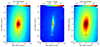 |
Fig. 1. HST/WFC3 images of NGC 4751 used to derive the galaxy luminosity profile; the galaxy nucleus is indicated with a black cross. Left: Original image from the F160W filter. Center: J′−H′ color map (see text) made by subtracting the F110W (J′) image from the F160W (H′) one; higher values trace regions with more dust. Right: F160W image as in the left panel, but now corrected for dust extinction (see Sect. 3.5). |
3. Galaxy properties
Our black hole mass measurement is based on the kinematics of the nuclear (out to ∼5″, with a few isolated emission line clumps detected out to ∼7″) CO disk. To better understand the stellar potential’s contribution to the rotation in the inner 5″, constraints on the larger-scale galaxy properties are required, especially the galaxy rotation curve. Thus, we first discuss the global morphology and kinematics of the galaxy below.
3.1. Galaxy morphology
NGC 4751 is listed in SIMBAD as having a Hubble stage T = −3 and an extent of 2′ × 0.8′ (from 2MASS imaging). NED lists this galaxy as having a Hubble – de Vaucouleurs morphological type of ‘SA0−:’ (from the RC3 catalog) or ‘SAO−:’.
HST images of NGC 4751 show multiple dust lanes on the western side of the galaxy, notable out to 15″ from the nucleus. Figure 2 shows 60″ and 20″ scale structures from the HST/WFC3 F160W image. To guide the eye, the stellar brightness is shown in color and selected contours, and ellipses in PA = 355° with inclinations of 65° and 78° are overplotted. From the left panel, it can be seen that the outer contours of the galaxy light (at radii larger than ∼15″ along the major axis) are better fit with a circular disk with inclination close to 60°–65°. On the other hand, the dust lanes are better fit with a circular disk with inclination closer to 78°, as seen in the right panel of the figure. Further below, detailed fits to the morphology and kinematics will shed more light on these first visual impressions about the inclinations.
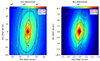 |
Fig. 2. F160W HST/WFC3 images of NGC 4751, with selected brightness contours shown in black. Left: Image covering a portion of the FOV; overplotted are four illustrative ellipses in PA = 355° with inclinations of 65° (red) and 78° (blue) and semi-minor axes of |


3.2. Global kinematic properties
The MUSE wide field data set covers the central 1′ of NGC 4751 and allows us to map the flux, velocity, and velocity dispersion, for both the stars (via pPXF) and emission line gas (via GANDALF). PV diagrams along relevant PAs also allow us to constrain the stellar dynamics and ionized gas kinematics. Additionally, the stellar population fits of pPXF reveal the best fit stellar populations and thus (weighted) mean age and metallicity values across the galaxy disk. Together, these allow us to determine the PA and inclination(s) of the components of NGC 4751, and constrain the M/L to be used to convert the stellar luminosity profile into an accurate mass profile (see Sect. 3.6) and, thus, a galaxy rotation curve.
The stellar intensity, velocity, and velocity dispersion maps, as obtained by running pPXF on the MUSE cube, are shown in the first, second, and fourth panels in Fig. 3. The important features to note are the dust lane across the western side of the galaxy in the intensity map (discussed in the previous section), the relatively symmetrical velocity field, and a dispersion, which peaks ∼1″ to the west of the nucleus. Given the dust lane running through the nucleus of NGC 4751, the stellar continuum peak cannot be used to define the kinematic center. We used internal scripts to determine the central pixel and central velocity, about which the global stellar velocity field is most symmetrical. The third panel of Fig. 3 shows the observed stellar velocity (i.e., the second panel) minus a model built using the KINematic Molecular Simulation tool (KinMS) of Davis et al. (2013). KinMS creates a simulated datacube based on an analytical, morphological, and kinematical model of the galaxy, and convolves it to the observed spatial and spectral resolution of the observation. To avoid using an “a priori” inclination, we explored the inclination range of 45°–55° in steps of 1°; the PA is fixed to 355°. The program SkySampler in KinMS was used to replicate the surface brightness of the stars by distributing about 2 million simulated clouds in such a manner that they fit the stellar intensity map. We set a spatially constant velocity dispersion of 10 km s−1. After creating the model in KinMS, we use the spectral-cube package in python to make the model velocity map. We then built the residual stellar velocity map (observed minus model) and chose the residual map with the minimum standard deviation. The result is that the model with an inclination of 52° is most favored. We remark that KinMS was used again later in this work, but the later applications exhibit substantial differences. The model and residual stellar velocity fields are discussed in Sect. 4. The residual velocity panel is placed here for easy visual comparison with the other panels of Fig. 3. Here, the fifth panel shows the derived mean age of the stellar population (in Gyr), based on the pPXF fits. We note that the color bar is highly “stretched”, that is, the stellar populations are relatively constant with radius, at least in the inner ±10″ along the major axis. The sixth panel shows the mean metallicity of the stellar population as derived with pPXF; the metallicity within ±5″ along the major axis is also relatively constant.
 |
Fig. 3. Stellar properties derived by running pPXF (in the GIST Pipeline) on the MUSE datacube. Left to right: Maps of the stellar log intensity, stellar velocity, stellar residual velocity (observed minus model; see Sect. 3.2), stellar dispersion velocity, median stellar population age (Gyr), and metallicity. The nuclear position and the major and minor axes are marked in each panel. We note that the peak of the stellar dispersion is offset (toward the dust lane) from the nuclear position. The stellar population age is the intensity weighted median stellar population age of all templates used to fit a given spaxel. |
The ionized gas kinematics obtained by GANDALF are shown in Fig. 4. The first, second, and fourth panels show the flux, velocity, and velocity dispersion of the [N II] λ6583 emission line. One can immediately note the east-west disk asymmetry in all panels. The gas is brighter, shows higher velocities, and larger dispersion, on the western half of the disk. The third panel shows a residual velocity map (observed [N II] velocity map minus the observed stellar velocity map). On the western (inner) half of the disk, the [N II] velocities exceed the stellar velocities by ±100 km s−1, while the eastern half and the outer western half show no significant deviations. A further remark on the morphology seen in this residual velocity field: while [N II] velocities can be traced across the full FOV shown in the figure, the excess velocity (and dispersion) ionized gas appears to trace the western half of a very high inclination disk, that is, its total extent more closely follows the i = 78° (instead of i = 65°) ellipse in Fig. 2.
 |
Fig. 4. [N II] λ6583 emission line properties derived using GANDALF (within the GIST Pipeline) on the MUSE datacube. Left to right: Maps of the [N II] log intensity, velocity, velocity residual (after subtracting the stellar velocity field), and dispersion velocity. The nuclear position and the major and minor axes are marked in each panel. |
For a more direct view of the emission line velocities, Fig. 5 shows pv diagrams, in PA 355°, of the [N II] λ6583 line: the central panel corresponds to a slit crossing the galaxy nucleus, and the left and right panels have slits with nuclear offsets of, respectively, −2″ and 2″. At this point we note that the observed pv diagrams in the offset slits are significantly different from each other. The eastern slit primarily traces the expected “S” shaped pattern of a single disk in pure rotation. However, the western slit (which crosses the dust features and thus the near side of the inner dusty disk) shows a broad range of velocities at nuclear offsets out to ∼12″. Two analytical velocity models are overplotted in each panel; these show the projected (for two inclinations) circular velocities expected from the black hole only, the galaxy potential only, and the sum of black hole and galaxy. A comparison of these models to the observed pv diagrams is presented in Sect. 4.
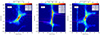 |
Fig. 5. Position-velocity diagrams of the [N II] λ6583 emission line along slits parallel to (but offset from) the major axis of the galaxy. Left to right: Offset by −2″ (i.e., to the east), 0″ (i.e., nuclear), and 2″ (i.e., to the west), from the nuclear position. Offsets along the slits (x axis) are measured from the intersection point of the slit with the minor axis of the galaxy; positive offsets are to the N side of the galaxy. Models overplotted in magenta and black follow the inclination listed in the legend; they have the black hole mass and M/L of our adopted best fit model (see Sect. 4). The black hole only (vbh) and total (vtot; galaxy plus black hole) radial velocity predictions are plotted in all panels; the galaxy prediction (vst) is plotted only in the central panel. |
3.3. Nuclear molecular disk properties
The 345 GHz continuum emission from NGC 4751 is clearly detected (left panel of Fig. 6), with a compact nuclear source, plus diffuse emission in a disk-like morphology, similar to that of the inner brighter CO emission. The continuum peak is at 12:52:50.744, −42:39:35.55 (J2000): in the following section we show that this position is consistent with the kinematic center of the molecular gas disk. The compact nuclear continuum source has peak flux 7.9 mJy/beam and integrated flux 9.16 mJy, with an extension of  ×
×  (∼30 pc) in PA 150°. The total continuum flux detected is ∼37 mJy, that is, there is about 28 mJy of diffuse continuum emission from the inner CO emitting disk. The latter flux density is highly uncertain as the emission is diffuse and detected at low S/N in individual pixels. Further the ALMA antenna configuration used for this observation does not recover the continuum emission from structures with scale ≳3″. In view of the relatively high observing frequency, the diffuse continuum emission from the disk is expected to originate from dust. Given the 5 GHz flux of 3 mJy (epoch 1988) detected by Sadler et al. (1989) in the inner 3″ of NGC 4751, the compact nuclear 345 GHz emission is unlikely to be due to synchrotron emission from a jet, unless the nucleus has significantly brightened (factor 20 in case of optically thin synchrotron emission) since 1988. If the continuum emission comes from dust, the scaling relationships of Orellana et al. (2017) predict a dust mass of 2.3 × 10⁶ M⊙ for the compact nuclear source, and a diffuse dust mass (over the line emitting disk) of at least 7 × 10⁶ M⊙. Alternatively, this compact mm emission comes from an advection dominated like accretion inflow (e.g., Ramakrishnan et al. 2023).
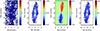 |
Fig. 6. Maps of the 345 GHz continuum (mJy), and the CO J:3−2 emission line moment 0 (flux; Jy km s−1), moment 1 (velocity; km s−1), and moment 2 (velocity dispersion; km s−1) in NGC 4751. All panels follow the color bar on their right and share the same center and FOV. The “zero” velocity corresponds to 2130 km/s and the cross marks the position of the continuum peak. While most of the CO emission was detected inside the FOV shown here, a few isolated clumps are detected up to 7″ from the nucleus. |
The integrated intensity map of the CO J:3−2 emission (Fig. 6) shows that the inner molecular gas disk is  ×
×  in extent. Assuming intrinsic circularity, this implies a (morphological) inclination of 77°. The total CO J:3−2 flux in the disk is 53.4 Jy km s−1. At our assumed distance, this translates to
  = 1.3 × 10⁴ L⊙ for the CO J:3−2 transition. Using a standard αCO = 4.6 (Bolatto et al. 2013), and assuming that the CO J:3−2 to CO J:1−0 luminosity ratio is 0.27 as in our Galaxy (Carilli & Walter 2013), this implies a total molecular gas mass of 2.2 × 10⁵ M⊙. The CO moment 0 image shows an inner
  hole and relatively bright CO emission at radii of
  to
to  both north and south of the nucleus. Over these radii, the southern half of the disk is brighter (peak flux of 1.6 Jy km s−1) than the northern half (peak flux of 1.3 Jy km s−1). Further out the CO emission is weaker and somewhat filamentary. Thus the true extent of the disk is best appreciated in the moment 1 (velocity) image shown in the third panel of Fig. 6, and in the pv diagrams shown in Sect. 4. The moment 1 map clearly shows that the disk is symmetric in velocity, and dominantly in rotation, with major axis PA near ∼355°. The highest velocities (around ±660 km s−1) are seen at the smallest radii, a clear indication of the effect of the SMBH. The moment 2 map of the disk (rightmost panel of Fig. 6) reveals an unusual hourglass shape of apparently high “velocity dispersion”, effectively extending over the full disk, though most notable in the inner 1″ − 2″. We immediately noted that this pattern does not necessarily trace non-circular kinematics. In Sect. 4, we show that this is an observational artifact due to “beam smearing” effects when observing highly inclined rotating disks. Outside this hourglass figure, the true disk dispersion is unresolved by our observations.
Given the hourglass artifact, deriving disk kinematic parameters via typically used “inverse” methods are not reliable, since those methods typically derive kinematic parameters, either from the observed velocity field or the full datacube, by fitting individual tilted rings of increasing radius. Nevertheless, for initial constraints on the major axis PA and inclination, and for a thorough investigation of these artifacts, we use Kinemetry (Krajnović et al. 2006) on the velocity field (see Sect. 3.4).
Figure 7 shows two selected pv diagrams of the ALMA cube along two slits symmetrically offset from the major axis of the galaxy. Similar to the left and right panels of Fig. 5, the left and right panels show pv diagrams along slits in PA 355°, but with offsets from it of 0.6″ to the east (−0.6″) and 0.6″ to the west, respectively. Unlike the case of [N II], the observed CO pv diagrams here both show the expected “S” shape curves. That is, both the eastern and western sides of the CO disk appear to follow the same rotation dominated behavior without significant east-west asymmetry in velocity or inclination. In each panel, we also overplot the projected velocities expected from analytic models of rotation with only a black hole and with a black hole plus galaxy potential (black lines). The comparison between the observed pv diagrams and the modeled velocities is deferred to Sect. 4.
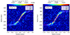 |
Fig. 7. Same as Fig. 5, but with the position-velocity diagrams of the CO emission line set along slits parallel to (but offset from) the major axis (PA 355°) of the galaxy. Left to right: Offset by −0 |


3.4. Galaxy properties from Kinemetry
We used the Kinemetry package to fit the PA and inclination of the stellar light in the HST/WFC3 F160W image and the MUSE WFM moment 0 map. The results are similar, so we discuss and present only those of the HST image as it has a higher resolution and extends to larger radii. The best fit PA is stable with increasing radius, and always within a few degrees of 355°. We therefore fix this value of PA, and fit only the inclination of the disk with Kinemetry. The results are shown with the black connected points in the left panel of Fig. 8. Fit results in the inner 15″ (dashed connectors) are clearly incorrect when revising the output figures of Kinemetry. This is due to the prominent dust features, however, results at larger radii (solid connectors) are visually reliable. Effectively, at radii beyond ∼15″, NGC 4751 can be explained morphologically as an inclined circular disk with inclination ∼65°. Alternatively, the observed ellipticity is due to the projection of a tri-axial bulge.
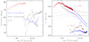 |
Fig. 8. Results from Kinemetry. Left: Best-fit kinematic inclination as a function of nuclear distance obtained by Kinemetry on the CO (red), [N II] λ6583 (brown), and stellar (blue) velocity fields, with the PA fixed to 355°. For reference, the equivalent (morphology) results from running Kinemetry on the HST/WFC3 F160W image are shown in black; at radii ≤15″ these latter fits are not reliable, due to the prominent dust lanes, and are shown with a dotted black line. Error bars are as reported by Kinemetry. Right: Kinemetry-derived k1 coefficient (the – projected for inclination – amplitude of the “pure-rotative” component k1 cos θ) as a function of radius when fitting the velocity fields of CO (red symbols), [N II] λ6583 (brown symbols) and stars (blue symbols). Error bars shown are as reported by Kinemetry. Overlaid (see Sect. 4) are the adopted best fit inclination-projected rotation curves due to the stellar potential for the arctangent (brown dotted lines) and the MGEFit solution (blue dotted lines): two curves (inclinations of 78° and 65°) are shown for each. The solid lines in the corresponding colors show the total expected inclination-projected rotation curve if our adopted best-fit value (3.34 × 10⁹ M⊙) for the black hole mass is considered. |
We also fit the PA and inclination of the velocity maps of the ionized and molecular gas with Kinemetry. As for the stellar light, the best fit kinematic PA is highly stable with radius and within a few degrees of 355°, and we fix this value in Kinemetry so that the inclination is the only free parameter. The resulting best fit kinematic inclinations as a function of nuclear distance are shown in the left panel of Fig. 8. The inclination of the CO disk is relatively stable, especially over ∼1−5″, where sufficient pixels are included in each annular fit. The favored inclination is i = 78° ± 2°. The reliability of this value is confirmed by the off-nuclear CO pv diagrams presented in Fig. 7. The kinematic inclination of the stellar and [N II] velocity fields show larger variations and imply lower values.
We recall that (as seen in Fig. 2) at a nuclear distance of 11″ along the major axis the galaxy, contours are reasonably well explained by a circular disk with inclination i ∼ 65°, while inside a nuclear distance of  along the major axis the dust lanes are better fit with a circular disk with i ∼ 78°. In both cases – low and high inclination disks – the PA of the disk remains constant at ∼355°.
The right panel of Fig. 8 intercompares the Kinemetry derived k1 component (the projected amplitude of the rotation velocity) of the CO, [N II], and stars. These are compared to rotation curves used in sections further below. NGC 4751 thus appears to have a dusty (and molecular gas rich) disk with i ∼ 78° which can be discerned out to a semi-major axis of  in the near-IR (and out to ∼5″ in CO J:3−2), and a primary stellar disk with i ∼ 65° over the semi-minor axis range 11″ and beyond. The near side of the inner dusty disk is to the west; here clear dust lanes are seen where the high inclination disk obscures stars in the lower inclination stellar disk.
We now focus on the Kinemetry results for the CO line, in order to constrain the major axis PA and inclination of the disk, and the rotating and non-rotating velocity components present. When running Kinemetry, we fixed the central position to that of the 345 GHz continuum source, allowed both the major axis PA and the disk inclination to vary with radius, and used both odd and even terms in the Fourier expansion: cos(nθ) and sin(nθ) with n = 1, 2, 3, 4. The relevant results are shown in Fig. 9, with the fitted major axis PA and disk inclination in the left panel and the amplitude of the rotating (cos θ) component and the ratio of the amplitudes of the non-rotating to rotating components in the right panel. For illustration, we performed fits out to ∼6″, even though beyond 4″ the velocity data are relatively sparse and so the results are not reliable.
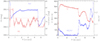 |
Fig. 9. Parameters of the CO disk as determined by Kinemetry. Left: Fitted major axis PA (red; left y axis) and inclination (blue; right y axis) as a function of radius. Right: Kinemetry derived k1 coefficient (red: the amplitude of the “pure-rotative” component k1 cos θ projected for inclination; left y axis), and k5/k1 (blue: the ratio of the sum of the amplitudes of the non-rotative components – cos(nθ) and sin(nθ) for n = 1, 2, 3, 4 – to k1; right y axis) as a function of radius. Error bars shown are as reported by Kinemetry. The stability of all values in both panels over the radius range |

The fitted major axis PA is relatively invariant out to 5″, with a median value of 355°, the same as the value derived from the morphology of NGC 4751. From now on we use this value as the major axis PA. The fitted inclination shows a roughly constant value of 78° (in agreement with the morphological inclination) between 2″ and 4″, but lower values in the inner 2″. The sudden increase in inclination at the smallest radii is likely a numerical effect as very few independent pixels are available for ring fitting at these radii. The decrease in inclination in the  to 2″ range is most likely an effect of the high-dispersion hour-glass figure mentioned above (as we see below, this hourglass traces areas with beam-smeared velocity profiles, which likely bias the Kinemetry fits). The k1 term represents the (projected) amplitude of the pure rotation component (cos θ), that is, the rotation curve: this is observed to be smoothly varying out to
  . The k5/k1 ratio shows that rotation dominates at all radii, but that significant non-circular motions are present in the inner 1″, and beyond
  . The former is once more likely a result of the hourglass figure in dispersion, and the latter most likely due to the sparse velocity coverage at larger radii. In subsequent Kinemetry runs, we fixed both the major axis PA (355°) and inclination (78°). The resulting rotation curves and ratio of non-circular to circular motions show some changes. Specifically, non-circular motions are now negligible between
  and 4″. We also found that the strong non-circular motions found by Kinemetry in the inner arcseconds cannot be decreased by lowering the disk inclination.
The stability of the values of the major axis PA and inclination of the CO disk (at least over radii not biased by the hourglass artifact) and their close agreement to the morphologically derived equivalents make these values robust. Furthermore, given the disk is close to edge on, the very small errors in these two values do not affect our estimations of the M/L and SMBH mass in the following sections. That is to say that the radial velocity, projected with sin(78°), does not change significantly for a variation of a few degrees in the major axis PA or inclination. We thus fixed both PA and inclination to these values in our principal fitting runs in the next section. However, we also performed fitting runs with the inclination as a free parameter to estimate the error budget when assuming this fixed value.
3.5. Correction for dust extinction
To derive an accurate rotation curve from the stellar component of NGC 4751, we first built a color map using both the F160W and F110W HST/WFC3 images (see Sect. 2.3) and used it to compensate for dust extinction effects in the galaxy using multiple approaches: (a) masking regions highly affected by extinction; (b) correcting the F160W image for dust extinction, and (c) both of the above.
Hereafter, we refer to the magnitude in the WFC3 F110W filter as J′, and the magnitude in the WFC3 F160W filter as H′. The J′−H′ (F110W−F160W) color map, which traces both the intrinsic color of the galaxy components and the dust extinction, is thus constructed as:
 (1)
(1)
where fF110W and fF160W are the F110W and F160W fluxes, respectively.
The resulting color map is shown in the central panel of Fig. 1. We note the region to the western side of the galaxy with an extension of about 28″ × 3″, where the color values are high (above ∼ − 0.5). Given the roughly symmetric disk-like shape of the extended 230 GHz continuum emission, the obvious interpretation is that the near side of the (dusty) disk obscures the light from the bulge on the W half of the galaxy.
We use the derived color map to build a extinction-corrected version of the F160W image. The procedure begins by assuming that the extinction A is a linear function of J′−H′:
 (2)
(2)
where a0 and a1 are unknown parameters. The flux in the corrected image, fF160W, corr, is calculated as follows:
 (3)
(3)
We refer to the value of 10−0.4A in Eq. (3) as the dust extinction correction factor. Inserting Eq. (2) into (3) allows us to express fF160W, corr explicitly as function of a0 and a1:
 (4)
(4)
We can then proceed to find the best-fit values of a0 and a1 separately in two steps: (a) looking for a value of a1 for which the corrected image is as symmetrical as possible with respect to the galaxy major axis; and (b) looking for a value of a0 for which the regions far from the nucleus are as similar as possible in the original and corrected images. In both cases, we use a minimization algorithm as described below.
In order to find a1, we build a mirror image of both the original and the color map images (i.e., images reflected with respect to the major axis), that we call fF160W, MI and (J′−H′)MI respectively, and use them to obtain a mirror image of the corrected image fF160W, corr, MI as follows:
 (5)
(5)
The objective function of the minimization is the difference between the corrected map in Eq. (4) and the mirror image of it in Eq. (5):
 (6)
(6)
After replacing Eqs. (4) and (5) in (6), we divide it by 10−0.4a0 since it is constant over the image (i.e., it does not depend on the color); the resulting expression depends only on a1:
 (7)
(7)
Using the “least_squares” function from the Python package SciPy, we find that a1 = −3.3071 minimizes the objective function.
To find a0, we set the objective function as the difference image (original minus corrected image; both in units of electrons/s). Pixels with fluxes greater than 0.8 electrons/s in the original image (i.e., the bright nuclear regions; see the left panel of Fig. 1) are masked in the difference image. Thus, effectively, only regions far from the nucleus (≥30″ along the major axis, and thus outside the FOV of the figure shown) are used in the difference image (i.e., objective function). Once more using “least_squares” we find that a0 = −2.3641 minimizes the objective function.
The dust extinction corrected F160W image, built using Eq. (3), is shown in the right panel of Fig. 1, and has the same color scale than the original image (left panel of the same figure). An important feature seen when comparing both images is that the flux in the corrected image increases significantly with respect to the original in the inner ∼30″. The effect of this increase on the estimated SMBH mass or M/L (or both) is explored in Sect. 4.
3.6. Galaxy luminosity profile
Constraining the luminosity profile and M/L of the host galaxy is a crucial ingredient of a reliable black hole mass measurement. The molecular gas disk is relatively compact in NGC 4751; it alone cannot be used to fully constrain the contribution of the stellar potential to the overall rotation curve of the galaxy.
Rusli et al. (2013) used an image from the Near Infrared Camera and Multi-Object Spectrometer 2 (NICMOS2) aboard HST, taken with the filter F160W (Proposal ID: 11219, PI: A. Capetti) to constrain the galaxy potential for their measurement of the black hole mass via stellar dynamics. This image has a FOV of about 20″ × 20″, which covers the full CO emission line region in the ALMA datacube, but not the full [N II] emission line region in the MUSE datacube. While HST/NICMOS2 has a higher spatial sampling, we decided to use the more recent HST/WFC3 F160W image in our analysis (which has a lower spatial sampling of  as compared to
  for the NICMOS2 image), since its FOV is larger (see Sect. 2.3), and encompasses both the CO and [N II] emission line regions. Full coverage of the galaxy is especially important when the radial mass profile of the galaxy is derived via nested Gaussian fitting to the brightness contours. To better understand the errors introduced by dust extinction in the following procedure, we used both the original and dust extinction-corrected WFC3 images, with and without masking regions highly affected by dust extinction.
Given the clear dust extinction seen toward the near (W) side of the galaxy disk, we applied independent dust masks to each (observed or corrected) WFC3 image, so that the fits would be performed only on the (relatively) un-extincted parts of the galaxy.
For the original observed WFC3 image, the following masks were applied: (a) excluding the eastern half of the galaxy (hereafter “half mask”), where most of the dust extinction is seen; and (b) excluding pixels with dust extinction correction factor 10−0.4A greater than 1.2 (hereafter “dust mask”). We note that values of 1 imply no corrections, while larger values imply larger extinction corrections. The masked regions for both cases can be seen in yellow in the left and central panels of Fig. 10; there, the black contours trace the (observed or corrected) image brightness profile and the red contours show the best fit results from MGEFit.
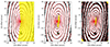 |
Fig. 10. Brightness contours of NGC 4751 in the HST/WFC3 F160W (original or corrected) image (black) overlaid with the contours from the (3D) multi-Gaussian fit (red); the relatively dust-obscured regions of the galaxy (yellow shaded) were excluded from the fitting. Left panel: Original F160W image with the “half mask” applied. Central panel: Original F160W image with its respective “dust mask” applied. Right panel: Corrected F160W image with its respective “corrected dust mask” applied. |
For the extinction corrected WFC3 F160W image: (a) no region is excluded (hereafter “corrected no mask”); and (b) pixels with a dust extinction correction factor 10−0.4A greater than 1.6 (hereafter “corrected dust mask”) are excluded. Note that this value of 1.6 is larger than the cutoff used for the “dust mask” above, that is, fewer regions are now masked since we expect that the dust correction worked over the range 10−0.4A of 1−1.6. The unused region for the last case appears shaded in yellow in the right panel of Fig. 10.
We fit each image with the MGE-Fit-Sectors method (hereafter MGEFit), which obtains a Multi-Gaussian Expansion parameterization for the galaxy surface brightness (Emsellem et al. 1994; Cappellari 2002). MGEFit uses the routine “find_galaxy” to compute the center, orientation and ellipticity of the image; then “sectors_photometry” to divide the galaxy into a grid of sectors spaced in angle and radius; and finally “mge_fit_sectors” to parameterize the photometry as the sum of two-dimensional Gaussian profiles. In each run we set the maximum number of Gaussians to 20, use a sigma point-spread-function (PSF) of 0.4 pixels, and set the “bulge_disk” option as true in order to perform a non-parametric bulge/disk decomposition.
An example fit to the surface brightness profile and its components is shown in Fig. 11, corresponding to the observed F160W image with its “dust mask” (i.e., the case of the central panel of Fig. 10); the curves in the central panels are the profiles along the major (top panel) and minor (bottom panel) axes of the galaxy. Systematic differences between model and data are seen along both the major and minor axes, with systematic trends with radius at the ≲15% level. We note that only two example cuts are shown, while the fitting minimization was performed in two dimensions (i.e., all PAs).
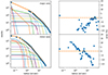 |
Fig. 11. Example results of the (3D) multi-Gaussian fit to the HST/WFC3 F160W image. Here we show results for the original F160W image with its dust mask applied (central panel in Fig. 10). Left panels: Binned counts (blue filled circles) along the disk major (top) and minor (bottom) axes, the best fit summed profile (highest orange line), and the individual Gaussian profiles which feed into this sum (lines of various colors). Right panels: Corresponding percentage errors between counts and the best fit profile. |
The peak values of the Gaussians from MGEFit were converted from counts (in electrons/s) to surface density in units of L⊙/pc2. This conversion used an absolute magnitude of the sun in the ST system of 6.84 mag for the instrument WFC3 and the filter F160W (Willmer 2018), and followed a simplified version of the steps provided by the author in a README file distributed with MGEFit2. The resultant Gaussians, now in units of L⊙/pc2 are used to derive a galaxy circular velocity profile using the module “velocity_profs” in the KinMS package; this module uses the “mge_vcirc” routine from the JamPy package (Cappellari 2020) and a user-defined M/L ratio.
As noted by Cappellari (2002), if the deprojected (3D) mass distribution is assumed to be oblate axisymmetric, there is a minimum possible inclination for the MGEFit model, dictated by the Gaussian with the smallest ellipticity. While in previous sections we argued for a stellar disk inclination at large scales of 52°, the smallest ellipticity from our MGEFit results forced us to use an inclination of 66° (and in some cases 69°) when deriving the galaxy rotation curve. This fact likely introduces an additional systematic uncertainty in our black hole mass measurement; in the following section we explore the use of an alternative analytic rotation curve, independent of MGEFit, which helps shed light on the introduced uncertainty.
4. Black hole mass from CO kinematics
Having presented and discussed the overall galaxy morphology and kinematics above, along with our derivation of the radial stellar luminosity profile, we can proceed to estimate the black hole mass required to explain the observed CO kinematics.
The PV diagrams along the major (PA 355°) and minor (PA 265°) axes of the molecular gas disk are shown in Figs. 12 and 13, respectively. The gas disk is spatially well resolved along both PAs. Along the major axis CO emission is strongly and continuously detected out to radii of ∼4−5″ (∼500 pc) with weaker blobs of emission detected out to ∼7″. It is immediately clear that the kinematics change from Keplerian-like in the inner region to almost flat in the outer region: a clear indication that we have resolved the sphere of influence of the SMBH. This is, from the point of view of SMBH mass measurements, one of the most spectacular resolved molecular disks. Along the minor axis, CO emission is detected out to ±2″ (i.e., ∼8 synthesized beams) and shows velocities close to zero, as expected for pure rotation without significant contamination from non-circular kinematics. The large range of velocities seen near the nuclear position is in part due to beam smearing (as confirmed with KinMS simulated cubes), but could also be in part due to off-planar molecular gas whose true nuclear distance is significantly larger than its projected distance to the nucleus, an effect accentuated in a high inclination disk such as this. The models over-plotted in the major axis pv diagram use the best fit values found later in this section.
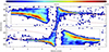 |
Fig. 12. PV diagram along the kinematic major (PA = 355°) of the molecular disk. The observed data are shown in color, following the color bar above the panel (units of Jy/beam), and small black dots in the panel mark the velocity channel in which the profile reaches maximum intensity for each x axis value. The star marks the position of the 345 GHz continuum. The inserts in the major axis pv diagram show zooms of the pv diagram for the innermost redshifted and blueshifted disk. Overplotted are our adopted best fit model: dashed lines show the predicted velocities for the galaxy potential and SMBH individually, while the solid lines shows the prediction combining both of the above. Black (red) is used for a disk inclination of 78° (65°). Note that the model traces the upper velocity envelope of the data at smaller radii; given the high inclination of the disk, the observed major axis “slit” samples other PAs (with lower projected velocities) in the inner arcseconds, underlining the need to use a software like KinMS for the best fit. |
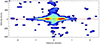 |
Fig. 13. Same as Fig. 12, but along the minor (PA = 265°) axis of the molecular disk, illustrating the lack of significant non-circular motions in the disk. |
As noted earlier, there is a central  hole in the CO J:3−2 traced molecular disk. Given that we significantly resolve the SMBH SOI, this is not a critical roadblock in measuring the black hole mass. In any case, emission lines from gas inside this radius would be smeared in velocity due to the spatial resolution of our observations, and the high inclination of the disk. We use the 230 GHz continuum source position as the first-guess kinematic center, and indeed find that this does provide the best results. A systemic velocity of 2130 km s−1 (36 km s−1 redder than the NED-listed recessional velocity) is required to center the kinematics of the molecular disk. The major axis PA and inclination are set to 355° and 78°, respectively, following the results of Sect. 3.3 (in a few fitting runs described further below, we leave the disk inclination as a free parameter in order to assess systematic errors due to fixing the inclination to 78°).
We forward model our datacubes using the KinMS package together with its extension for Monte-Carlo Markov Chain (MCMC) fitting: KinMS_fitter. The former produces a simulated datacube based on an analytical (or empirical) morphological and kinematical model for the galaxy, and the latter identifies the best-fit model by minimizing the difference between the observed and simulated datacubes as the (one to several) input model parameters are varied in a MCMC. Observational parameters including spaxel sizes, synthesized beam size, and velocity resolution, are taken from the observed datacube by KinMS. To avoid fitting to noise, all pixels in the observed datacube with fluxes ≤2σ were masked in the observed (and thus also the simulated) datacube.
We performed initial exploratory KinMS_fitter runs to test for variations in the kinematic center, recessional velocity, PA, inclination, and intrinsic velocity dispersion of the disk. Based on the results of these, we decided on the following values and constraints for the detailed KinMS_fitter runs: (a) KinMS_fitter best-fit PA values were always within two degrees of 355°, in agreement with the values derived from all kinematical and morphological fits described earlier. The PA was thus fixed to 355° in all runs, except for one KinMS_fitter run in which this was left as a free parameter; (b) KinMS_fitter best-fit inclination values were always within 2° of 78°, in agreement with the values derived from all kinematical and morphological fits described earlier. We therefore fixed the inclination at 78°, except for one KinMS_fitter run in which this was left as a free parameter; (c) KinMS_fitter best-fit central pixel position values for the CO disk are always within 1 pixel of the 230 GHz continuum peak. Given the spatial sampling of our cube (a  synthesized beam sampled at
  pixels) we fixed the central position of the disk to the 230 GHz peak flux position in all runs which did not use SkySampler (see below).
With the fixed parameters described above, we performed several detailed KinMS_fitter runs with permutations of the following inputs (noting that the black hole mass, velocity dispersion, recessional velocity, and total CO flux were always kept as free parameters):
-
Two options for the surface brightness of the disk: (a) an axisymmetric exponential disk brightness profile, with a central hole. This model, included in KinMS_fitter, was used with two free parameters: the exponent of the disk (Rscale_exp) and the outer radius of the central hole (End_cutoff). The disk center was fixed to the 230 GHz continuum peak position; (b) a brightness profile produced by the function SkySampler, included in KinMS_fitter (see Sect. 3.2). Here the sampling is based on the morphology of the moment 0 image of the CO emission, with their brightness weighted to follow the intensity seen in the moment 0 image (option “inClouds_intensity”). This sampling intrinsically allows for variations in the central position of the disk.
-
Five options for the rotation velocity due to the galaxy potential: (a) an arctangent model for the galaxy rotation curve (a function built into KinMS_fitter) with free parameters “Vmax” and “Rturn” (the maximum achieved velocity in km/s and the turnover radius of the arctangent function in arcsec), as follows:
 (8)
(8)then, (b) four galaxy rotation curves derived from the results of a MGEFit fit to the observed or modified HST/WFC3 image, with the mass to light ratio (M/L; constant with radius) as a free parameter. The four MGEFit results used are those derived from (see Fig. 14 and Sect. 3.6): (b1) the observed HST/WFC3 image but with the W side masked (“half mask”); (b2) the observed HST/WFC3 image but with regions of high dust extinction masked (“dust mask”); (b3) the “dust corrected” HST/WFC3 image with no masking applied (“corrected no mask”); and (b4) the “dust corrected” HST/WFC3 image with masking applied to the dustiest regions (“corrected dust mask”).
We also performed four additional runs: three with fixed values of M/L, and one in which the disk inclination (constant with radius) is allowed to vary. These four additional runs use the brightness profile from SkySampler, and the rotation curve derived by MGEFit on the HST/WFC3 image with the “dusk mask”. The details and discussion of these additional runs are explained later in this section.
The resulting best fit values of SMBH mass and M/L from the runs with velocity profiles coming from the different permutations of MGEFit (original or corrected image, mask, and surface brightness) are shown in the first four rows of Table 1; the remaining results in that table, that is, the ones for the arctangent model, are presented and discussed further below.
Best fit M/L (F160W band) and SMBH mass values from different KinMS_fitter runs.
In what follows, we first compare separately the runs which use the original (i.e., non-dust-corrected) image, then the runs which use the corrected image, and finally all of them together. The results of the four runs which use the original image (first two rows in Table 1) are similar, with values in the range of 3.22−3.34 × 10⁹ M⊙ for the SMBH mass, and 2.264−2.294 for M/L. That is, the type of mask (half- or dust-) and the surface brightness profile (analytic or SkySampler) have a negligible impact on the resulting values. We note both that a larger region (as compared to that shown in Fig. 1) of the WFC3 image is used in MGEFit to derive the velocity profile, and that the use of SkySampler rather than an analytic SB involves fewer free parameters. Not all the above conclusions are valid when focusing on the results from runs using the corrected image (i.e., see third and fourth rows in Table 1). When the dust mask is not used, M/L tends to decrease by ∼10% and SMBH mass tends to increase by ∼26%, as compared to when the dust mask is used. We take this discrepancy as an indication that the corrected image has not yet completely corrected all the dust extinction. On the other hand, the choice of the SB profile (analytic or SkySampler) has a negligible impact on the SMBH mass. Finally, there are some important remarks to make when comparing the results from the original and corrected images. There is a big change in M/L, from values of ∼2.3 to ∼1.1. The effect on the SMBH mass seems to be unclear; to further explore that, it is worth noting that the SMBH mass from the result that uses the original image, SkySampler, and the “dust mask”, is in agreement with the one that uses the corrected image, SkySampler, and the “corrected dust mask”. In fact, other results in Table 1 are also in agreement with these runs. Therefore, we consider that the use of the original or corrected image impacts only the M/L value. The reason for the discrepancy between the M/L results can be appreciated by returning to Fig. 1. The fluxes in the corrected image (right panel) are higher than in the original image (left panel). In the former case, a smaller M/L ensures that the mass profile (therefore, the velocity profile) does not change significantly from that of the latter. We take this as an indication that there is an overcorrection of the dusk extinction; indeed, it explains why it makes a difference whether the masking is used or not in the corrected image. Since there are still unknowns regarding the correction of the F160W image for dust extinction, the subset of models which use the original image and a dust mask are likely the most reliable.
As mentioned in Sect. 3.6, we use an inclination in our MGEFit model greater than the stellar disk inclination from Sect. 3.2, that potentially introduces a systematic uncertainty. It can be partially evaluated via comparisons to the results when using the analytical (arctangent) rotation curve; these results are shown in the last row of Table 1. Once more, when comparing the two, it is noted that the choice of surface brightness (analytic or SkySampler) has a negligible effect on the results. The SMBH masses are however higher than those with the MGEFit-based velocity curves. This discrepancy can be explored with the aid of Fig. 14, which shows the arctangent and all the MGEFit-based velocity profiles. In what follows, we first compare the MGEFit curves to each other, and then compare them to the arctangent curve. Although the overall behavior of the MGEFit velocity curves are similar, some features can be noted. The “dust mask” (green) curve predicts higher velocities compared to the others up to  . That range is inside the sphere of influence of the black hole and should not affect the results to any great extent; it can be appreciated more clearly with the two dashed lines in the figure, corresponding to the velocity profiles originated from the minimum and maximum SMBH mass in our results (Table 1), whose values are greater than the galaxy velocity profiles up to
  . With respect to the “corrected no mask” (red) curve, it has smaller circular velocities in the range of
  . Since the galaxy velocities are comparable to the ones originated from the black holes, that range does affect the SMBH mass; in fact, a larger mass is needed to compensate the smaller velocities of that “corrected no mask” curve, which explains the results for this model. We now focus on comparing the arctangent (blue) curve with the others; with the “dust mask” (green) curve as example, the uncertainty in using MGEFit to derive the SMBH mass is explored. In the range
  , the MGEFit prediction is slightly greater than the arctangent one; this is, of course, compensated with a smaller SMBH mass in the fitting result. From
  the arctangent prediction tends to be constant and becomes increasingly separated from the MGEFit one. The behavior of the arctangent curve is intrinsic to the model, it should not be used to extrapolate the circular velocity far from the nucleus; this is specially important when comparing the resulting model to the [N II] emission line pv diagrams, where the flux extends up to 20″ − 30″ (see Fig. 5).
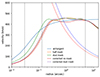 |
Fig. 14. Galaxy (projected) circular velocity profiles used here: the solid lines correspond to the results from MGEFit, each one with its respective model indicated in the legend; the dashed lines are Keplerian profiles as originated from a SMBH with masses of 3.22 × 10⁹ M⊙ (red line) and 4.33 × 10⁹ M⊙ (blue line); the vertical dotted lines are (from left to right) the ALMA pixel size ( |


Figure 15 shows the corner plots of the parameters fit for the arctangent model. In the top left panel, the pv diagram along the major axis of the ALMA data (in colors, red in the region where the flux is greater) and the best-fit result (black contours) are compared; the KinMS result seems to represent well the data, except in the inner  . Figure 16 also shows the corner plots and the pv diagrams comparison, but for our adopted result. The pv diagrams show a better fit than the arctangent result, specially in radii greater than 4″, where the arctangent model (in Fig. 15) does not fit the bubbles seen. Other features are worth noting in the corner plots. Most parameters in Fig. 15 (i.e., for the arctangent model) seem to be uncorrelated, except for a correlation between “Rturn” and SMBH mass, which would imply a ±3% uncertainty in black hole mass. Something similar occurs in Fig. 16 (i.e., for our adopted model): M/L appears to be inversely correlated to the SMBH mass, which would imply a ±1.5% uncertainty in black hole mass.
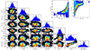 |
Fig. 15. Corner plots of the parameters fit with KinMS fitter using a galaxy circular velocity profile parameterized with an arctangent curve with free parameters Vmax and Rturn. The pv plots on the top right compare the data (colors) with the best-fit model (contours) along the major axis. |
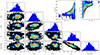 |
Fig. 16. As Fig. 15 but for our adopted result (galaxy circular velocity profile based on the results from MGEFit applied to the HST/WFC3 image together with the “dust mask”, and surface brightness profile from SkySampler). The mass to light ratio (M/L) is a free parameter here (in contrast to fitting with the arctangent model). |
With the KinMS_fitter results in hand, it is relevant to revisit the ionized emission line pv diagrams in Fig. 5; all of them are in PA = 355°; the plot in the central panel crosses the galaxy nucleus, and the plots in the left and right panels have offsets of 2″ to the east and 2″ to the west, respectively. The black solid line is the projected total velocity of a 78° disk whose potential comes from the stellar population (i.e., the velocity profile of our adopted result) and the SMBH; the magenta line is for a inclination of 52°. In the central panel, the 78° line appears to better fit the data; it can be noted even up to 20″ from the nucleus. In both offset panels neither of the models uniquely fit the data, although each does better than the other in certain regions. In the left panel (offset to the east), the 78° disk fits better than the 52° disk, though primarily in positive offsets (to the north) rather than negative, due to a small asymmetry in the data. The pv diagram in the right panel (offset to the west) traces the dusty region of the galaxy, and shows a larger velocity in the data than the models to the north; also, close to the nucleus, the 52° disk seems to fit better.
In order to test the overall consistency of the best fit M/L, we use the stellar isochrone tool CMD 3.73. This program estimates the integrated magnitude of a stellar population, given its age and metallicity, as well as the photometric system used. Taking advantage of the stellar population age and metallicity maps (Fig. 3), we use their values in the central Voronoi bin, as well as those in bins farther from the center along the major axis, to estimate M/L in the F160W filter using CMD 3.7. In the central bin (stellar population age = 13.4 Gyr, metallicity = 0.354) the resulting M/L is 2.537. This is slightly larger than our best fit result from KinMS_fitter, probably due to the presence of older stellar populations in the dispersion dominated region close to the nucleus. In the bins farther from the nucleus, the tool predicts M/L values of 2.198 (stellar age = 10.7 Gyr, metallicity = −0.189) and 2.289 (stellar age = 11.5 Gyr, metallicity = −0.144). These predicted values are in reasonable agreement with our results. All M/L values were calculated considering a solar luminosity magnitude of 3.37 mag in the Vega photometric system (Willmer 2018).
To test the uncertainties associated to the stellar population age and metallicity, we made three additional KinMS_fitter runs, but fixing M/L to the three values presented above. The results are shown in the first three rows of Table 2. The changes in SMBH mass when fixing the M/L to their GIST-estimated values far from the nucleus are of 0.5% and 10%. The biggest change in the SMBH mass (30%) occurs when setting M/L to the GIST-estimated value in the central bin of the MUSE cube. These of course represent extreme cases where all the stars contributing to the galaxy potential are considered the oldest or the youngest seen on the stellar moment maps. And the fact that they do not change the mass significantly lends further support to the robustness of our value.
Results from additional KinMS_fitter runs on the CO datacube.
In all previous fitting runs, the disk PA and inclination were fixed to 78° and 355°, respectively. We performed two additional runs: one with the inclination set as a free parameter (but constant with radius), and one with both PA and inclination as free parameters (but both constant with radius). Both runs used SkySampler and the rotation curve from MGEFit applied to the original F160W image with the dust mask. The results of the former run are tabulated in the last row of Table 2; here the best fit inclination is 79°, which produces a change of ∼1.5% in M/L and ∼3% in SMBH mass. When both PA and inclination are free parameters, the best fit PA and inclination are 354.9° and 79°, and thus the overall results are similar. The very small variation in projected velocities for inclinations within 1° of 78°, the robustness of the PA and inclination values derived by both KinMS_fitter and the kinematic- and morphological-based values presented in previous sections, and the reduction in free parameters (thus degrees of freedom) in KinMS_fitter, justifies our previous use of both PA and inclination as priors.
Finally, we return to the issue of the relatively low observed stellar rotation in the large-scale disk. Figure 17 shows the observed (deprojected) rotation velocity of the stars in black, as a function of the nuclear distance along the major axis. This rotation velocity was obtained by extracting velocities along the major axis of the stellar velocity map obtained from pPXF (second panel in Fig. 3), and deprojecting while assuming a disk inclination of 66°. The red line shows the intrinsic stellar velocity dispersion profile along the major axis, derived from the stellar moment 2 map obtained by pPXF (fourth panel in Fig. 3). This moment 2 map traces a combination of the true velocity dispersion of the stars together with gradients in the rotation velocities which are smeared due to the spatial resolution of the cube. To correct for the latter, we used KinMS to create a synthetic datacube, using as inputs the circular velocity curve from our adopted model, and a constant dispersion of 10 km s−1 (that is negligible compared to the true stellar dispersion). The moment 2 values along the major axis were extracted from both the observed and the simulated moment 2 maps and these were subtracted in quadrature to obtain the intrinsic stellar dispersion profile along the major axis, shown with the red line. Finally, the blue line in Fig. 17 shows the expected (deprojected) rotational velocity profile along the major axis. For this we used KinMS to construct a synthetic datacube using the best fit parameters of our adopted model (but without a black hole). A simulated moment 1 image was made from this synthetic cube, and then the velocities extracted along the major axis were deprojected for a disk inclination of 78°.
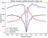 |
Fig. 17. Comparison of observed and expected stellar velocities, and the stellar velocity dispersion, along the major axis of NGC 4751. The blue line shows the predicted circular velocity extracted from a KinMS model built using of parameters of our adopted result (see text for the details). The black line shows the (deprojected for an inclination of 66°) velocity of the stars, and the red line the velocity dispersion of the stars. |
We observe in the figure that the dispersion increasingly dominates with decreasing nuclear distance, with a cross-over in magnitude at  . Given the signal to noise ratio in the stellar absorption lines we were unable to fit two components (bulge and disk) to the stellar absorption lines in pPXF so that the final (one component) stellar velocity map likely underestimates the true stellar rotation. In any case the difference between the blue (expected) and black (observed) stellar rotation curves is relatively large, which casts some doubt on the results when using the MGEFit plus HST/WFC3 models, and their implied galaxy rotation curves. A more reliable decomposition (using both morphology and dynamics) of the stellar bulge and stellar disk is required to fully confirm the validity of our SMBH mass estimations from the MGEFit-derived velocity curves. Fortunately, two factors mitigate these uncertainties: (a) a few isolated clouds of CO are seen out to ∼7″, so that the CO disk partly samples both the black hole SOI and a relatively galaxy-dominant rotation. Both regions fit well with our best fitting results; (b) the arctangent rotation curve model, which provides an MGEFit-independent approach, gives results which are only 20% larger.
Given all the above, we adopt as our fiducial result the one from the run which uses the surface brightness generated from the observed distribution using the program SkySampler, and the velocity profile from the program MGEFit applied to the HST/WFC3 image (without correction) after masking the region highly obscured by dust (dust mask). The resulting SMBH mass and M/L are 3.34 ± 0.03 × 10⁹ M⊙ and M/L 2.282 ± 0.007, respectively, where the uncertainties correspond to those reported by KinMS_fitter. The justification for this fiducial choice is that it has a minimal number of free parameters and thus degrees of freedom, with the fixed parameters coming from relatively reliable priors. Our exploration of multiple options in our fits has explored other sources of uncertainty including the use of multiple options of MGEFit velocity profiles (with uncertainties in the inclination for the deprojection, and the extinction due to dust), the variation of M/L along the galaxy radius, and the disk inclination. In this parameter exploration, we obtained SMBH best fit masses in the range 3.22−4.33 × 10⁹ M⊙, and M/L ratios of 1.1−2.3 in the F160W band. We thus adopt uncertainties of 20% around the fiducial values of SMBH mass and M/L. Given this 20% error budget for a fixed distance, the uncertainty in the distance to NGC 4751 is likely the primary driver of its SMBH mass error budget.
We can now compare our derived SMBH mass with an estimation from a M–σ relationship. Rusli et al. (2013) noted that NGC 4751 is an outlier (to higher SMBH mass) in that relationship. A velocity dispersion of 349 km s−1 (Gültekin et al. 2011) and the M–σ relationship of Saglia et al. (2016) predict a SMBH mass of 3.7 × 10⁹ M⊙ for NGC 4751. This estimate is different from that in Gültekin et al. (2011) since we use a more recent M–σ relationship. The new CO-based SMBH mass presented here is significantly closer to this estimated value (9.8% smaller) as compared to the stellar-dynamic based measurement (Fig. 16 of Rusli et al. 2013), so that NGC 4751 is no longer an outlier in the M–σ relationship.
5. Conclusions
Our high-resolution ALMA observations of NGC 4751 have found a rotating kpc-scale molecular gas disk. The disk extends over radii of 40 pc to 500 pc (with a few clumps detected out to 1 kpc) and is spatially resolved along both the major and minor axes. The rotational velocities are in the range 400 km s−1–650 km s−1, while the intrinsic dispersion of the gas is ∼16 km s−1, that is, the disk is relatively “cold”. The rotational velocities show a sharp increase with decreasing radius and detailed fitting of this allows for a precise measurement of the mass of the SMBH. While the kinematics of the molecular disk is axisymmetric, the CO J:3−2 emission is brighter in the southern half of the disk. This fact, coupled with the presence of dust in the F160W image, precludes any reliable check for an offset between the kinematic and morphological centers of the galaxy. The kinematic center of the molecular disk agrees well with the position of the nuclear 345 GHz continuum source. Continuum emission at 345 GHz is detected both as a compact source in the nucleus and as diffuse emission over the brighter parts of the disk. Attributing the nuclear continuum peak to synchrotron emission requires strong variability over the period from 1998 to 2017. Attributing this to dust implies a very high dust to CO J:3−2 ratio at the nucleus. Either high densities suppress CO J:3−2 emission (the critical density for this transition is 7 × 104 cm3) or cold temperatures cause molecules to freeze onto dust grains.
Assuming a single M/L at all radii (a standard assumption in many such studies), we can leverage the CO kinematics, larger scale ionized gas kinematics, and HST/WFC3 imaging to constrain the black hole mass and M/L. In our fiducial run, we obtained M/L = 2.282 in the F160W filter (H-band) and a best-fit SMBH mass of (3.34 ± 0.03)×109 M⊙, where the quoted errors are 3σ. This best-fit M/L is consistent with the M/L predicted using the CMD 3.7 stellar isochrone calculator for the stellar population mean age and metallicity derived from our MUSE data. Equivalent runs, but with variations in the input parameters (dust correction and mask, M/L and inclination values, and the analytic and observed brightness distributions) resulted in a larger spread in the black hole mass and M/L values. The primary uncertainty here is the stellar mass profile (and, thus, the rotation curve), which is derived via nested Gaussian fits to the F160W image and where several assumptions about the geometry and inclination of the galaxy were made. An alternative approach of using an analytical function (in our case, an arctangent with maximum velocity and turnover radius as free parameters) for the galaxy rotation curve, yields a larger SMBH mass; namely: ∼4 × 10⁹ M⊙. In all cases, the CO based SMBH mass presented here is certainly higher by a factor of two (or more) than the previously published stellar dynamics based SMBH measurement. NGC 4751 is thus another case (e.g., Walsh et al. 2012, 2013) where gas- and stellar-kinematics yield significantly different SMBH masses. Distilling all the best-fit runs, we have finally adopted a SMBH mass of 3.3 × 10⁹ × (D/26.3) M⊙, where D is the assumed distance to NGC 4751 in Mpc, with an estimated 1σ error of 20%.
Acknowledgments
We acknowledge funding from ANID Chile via Nucleo Milenio TITANs (NCN2023_002), Fondecyt 1221421, and Basal FB210003. JO acknowledges support from the ANID/Scholarship Program/Doctorado Nacional/2017-21171690, and from the French Agence Nationale de la Recherche (ANR), under grant ANR-23-EDIR-0003 (project GRAFITY). CF acknowledges funding from the FONDECYT Postdoctoral grant 3220751. This paper makes use of the following ALMA data: ADS/JAO.ALMA#2016.1.01135.S. ALMA is a partnership of ESO (representing its member states), NSF (USA) and NINS (Japan), together with NRC (Canada), MOST and ASIAA (Taiwan), and KASI (Republic of Korea), in cooperation with the Republic of Chile. The Joint ALMA Observatory is operated by ESO, AUI/NRAO and NAOJ.
References
- Bacon, R., Accardo, M., Adjali, L., et al. 2010, Proc. SPIE, 7735, 773508 [Google Scholar]
- Barth, A. J., Boizelle, B., Darling, J. K., et al. 2016, Am. Astron. Soc. Meet. Abstr., 228, 103.05 [NASA ADS] [Google Scholar]
- Bittner, A., Falcón-Barroso, J., Nedelchev, B., et al. 2019, A&A, 628, A117 [NASA ADS] [CrossRef] [EDP Sciences] [Google Scholar]
- Boizelle, B. D., Barth, A. J., Walsh, J. L., et al. 2019, ApJ, 881, 10 [Google Scholar]
- Boizelle, B. D., Walsh, J. L., Barth, A. J., et al. 2021, ApJ, 908, 19 [NASA ADS] [CrossRef] [Google Scholar]
- Bolatto, A. D., Wolfire, M., & Leroy, A. K. 2013, ARA&A, 51, 207 [CrossRef] [Google Scholar]
- Cappellari, M. 2002, MNRAS, 333, 400 [NASA ADS] [CrossRef] [Google Scholar]
- Cappellari, M. 2017, MNRAS, 466, 798 [Google Scholar]
- Cappellari, M. 2020, MNRAS, 494, 4819 [NASA ADS] [CrossRef] [Google Scholar]
- Cappellari, M., & Copin, Y. 2003, MNRAS, 342, 345 [Google Scholar]
- Cappellari, M., & Emsellem, E. 2004, PASP, 116, 138 [Google Scholar]
- Carilli, C. L., & Walter, F. 2013, ARA&A, 51, 105 [NASA ADS] [CrossRef] [Google Scholar]
- Combes, F., García-Burillo, S., Audibert, A., et al. 2019, A&A, 623, A79 [NASA ADS] [CrossRef] [EDP Sciences] [Google Scholar]
- Davis, T. A., Alatalo, K., Bureau, M., et al. 2013, MNRAS, 429, 534 [Google Scholar]
- Davis, T. A., Bureau, M., Onishi, K., et al. 2017, MNRAS, 468, 4675 [NASA ADS] [CrossRef] [Google Scholar]
- Davis, T. A., Bureau, M., Onishi, K., et al. 2018, MNRAS, 473, 3818 [NASA ADS] [CrossRef] [Google Scholar]
- Dreyer, J. L. E. 1888, MmRAS, 49, 1 [Google Scholar]
- Emsellem, E., Monnet, G., & Bacon, R. 1994, A&A, 285, 723 [NASA ADS] [Google Scholar]
- Falcón-Barroso, J., Bacon, R., Bureau, M., et al. 2006, MNRAS, 369, 529 [Google Scholar]
- Gültekin, K., Richstone, D. O., Gebhardt, K., et al. 2009, ApJ, 698, 198 [Google Scholar]
- Gültekin, K., Tremaine, S., Loeb, A., & Richstone, D. O. 2011, ApJ, 738, 17 [CrossRef] [Google Scholar]
- Kabasares, K. M., Barth, A. J., Buote, D. A., et al. 2022, ApJ, 934, 162 [NASA ADS] [CrossRef] [Google Scholar]
- Krajnović, D., Cappellari, M., de Zeeuw, P. T., & Copin, Y. 2006, MNRAS, 366, 787 [Google Scholar]
- North, E. V., Davis, T. A., Bureau, M., et al. 2019, MNRAS, 490, 319 [Google Scholar]
- Onishi, K., Iguchi, S., Sheth, K., & Kohno, K. 2015, ApJ, 806, 39 [NASA ADS] [CrossRef] [Google Scholar]
- Onishi, K., Iguchi, S., Davis, T. A., et al. 2017, MNRAS, 468, 4663 [NASA ADS] [CrossRef] [Google Scholar]
- Orellana, G., Nagar, N. M., Elbaz, D., et al. 2017, A&A, 602, A68 [NASA ADS] [CrossRef] [EDP Sciences] [Google Scholar]
- O’Sullivan, E., Forbes, D. A., & Ponman, T. J. 2001, MNRAS, 328, 461 [NASA ADS] [CrossRef] [Google Scholar]
- Ramakrishnan, V., Nagar, N., Arratia, V., et al. 2023, Galaxies, 11, 15 [NASA ADS] [CrossRef] [Google Scholar]
- Ruffa, I., Davis, T. A., Cappellari, M., et al. 2023, MNRAS, 522, 6170 [NASA ADS] [CrossRef] [Google Scholar]
- Rusli, S. P., Thomas, J., Saglia, R. P., et al. 2013, AJ, 146, 45 [NASA ADS] [CrossRef] [Google Scholar]
- Sadler, E. M., Jenkins, C. R., & Kotanyi, C. G. 1989, MNRAS, 240, 591 [NASA ADS] [Google Scholar]
- Saglia, R. P., Opitsch, M., Erwin, P., et al. 2016, ApJ, 818, 47 [Google Scholar]
- Sarzi, M., Falcón-Barroso, J., Davies, R. L., et al. 2006, MNRAS, 366, 1151 [Google Scholar]
- Theureau, G., Hanski, M. O., Coudreau, N., Hallet, N., & Martin, J. M. 2007, A&A, 465, 71 [NASA ADS] [CrossRef] [EDP Sciences] [Google Scholar]
- van den Bosch, R. C. E. 2016, ApJ, 831, 134 [NASA ADS] [CrossRef] [Google Scholar]
- Vazdekis, A., Sánchez-Blázquez, P., Falcón-Barroso, J., et al. 2010, MNRAS, 404, 1639 [NASA ADS] [Google Scholar]
- Walsh, J. L., van den Bosch, R. C. E., Barth, A. J., & Sarzi, M. 2012, ApJ, 753, 79 [NASA ADS] [CrossRef] [Google Scholar]
- Walsh, J. L., Barth, A. J., Ho, L. C., & Sarzi, M. 2013, ApJ, 770, 86 [NASA ADS] [CrossRef] [Google Scholar]
- Willmer, C. N. A. 2018, ApJS, 236, 47 [Google Scholar]
All Tables
Best fit M/L (F160W band) and SMBH mass values from different KinMS_fitter runs.
All Figures
|
Fig. 1. HST/WFC3 images of NGC 4751 used to derive the galaxy luminosity profile; the galaxy nucleus is indicated with a black cross. Left: Original image from the F160W filter. Center: J′−H′ color map (see text) made by subtracting the F110W (J′) image from the F160W (H′) one; higher values trace regions with more dust. Right: F160W image as in the left panel, but now corrected for dust extinction (see Sect. 3.5). |
| In the text | |
|
Fig. 2. F160W HST/WFC3 images of NGC 4751, with selected brightness contours shown in black. Left: Image covering a portion of the FOV; overplotted are four illustrative ellipses in PA = 355° with inclinations of 65° (red) and 78° (blue) and semi-minor axes of |
| In the text | |
|
Fig. 3. Stellar properties derived by running pPXF (in the GIST Pipeline) on the MUSE datacube. Left to right: Maps of the stellar log intensity, stellar velocity, stellar residual velocity (observed minus model; see Sect. 3.2), stellar dispersion velocity, median stellar population age (Gyr), and metallicity. The nuclear position and the major and minor axes are marked in each panel. We note that the peak of the stellar dispersion is offset (toward the dust lane) from the nuclear position. The stellar population age is the intensity weighted median stellar population age of all templates used to fit a given spaxel. |
| In the text | |
|
Fig. 4. [N II] λ6583 emission line properties derived using GANDALF (within the GIST Pipeline) on the MUSE datacube. Left to right: Maps of the [N II] log intensity, velocity, velocity residual (after subtracting the stellar velocity field), and dispersion velocity. The nuclear position and the major and minor axes are marked in each panel. |
| In the text | |
|
Fig. 5. Position-velocity diagrams of the [N II] λ6583 emission line along slits parallel to (but offset from) the major axis of the galaxy. Left to right: Offset by −2″ (i.e., to the east), 0″ (i.e., nuclear), and 2″ (i.e., to the west), from the nuclear position. Offsets along the slits (x axis) are measured from the intersection point of the slit with the minor axis of the galaxy; positive offsets are to the N side of the galaxy. Models overplotted in magenta and black follow the inclination listed in the legend; they have the black hole mass and M/L of our adopted best fit model (see Sect. 4). The black hole only (vbh) and total (vtot; galaxy plus black hole) radial velocity predictions are plotted in all panels; the galaxy prediction (vst) is plotted only in the central panel. |
| In the text | |
|
Fig. 6. Maps of the 345 GHz continuum (mJy), and the CO J:3−2 emission line moment 0 (flux; Jy km s−1), moment 1 (velocity; km s−1), and moment 2 (velocity dispersion; km s−1) in NGC 4751. All panels follow the color bar on their right and share the same center and FOV. The “zero” velocity corresponds to 2130 km/s and the cross marks the position of the continuum peak. While most of the CO emission was detected inside the FOV shown here, a few isolated clumps are detected up to 7″ from the nucleus. |
| In the text | |
|
Fig. 7. Same as Fig. 5, but with the position-velocity diagrams of the CO emission line set along slits parallel to (but offset from) the major axis (PA 355°) of the galaxy. Left to right: Offset by −0 |
| In the text | |
|
Fig. 8. Results from Kinemetry. Left: Best-fit kinematic inclination as a function of nuclear distance obtained by Kinemetry on the CO (red), [N II] λ6583 (brown), and stellar (blue) velocity fields, with the PA fixed to 355°. For reference, the equivalent (morphology) results from running Kinemetry on the HST/WFC3 F160W image are shown in black; at radii ≤15″ these latter fits are not reliable, due to the prominent dust lanes, and are shown with a dotted black line. Error bars are as reported by Kinemetry. Right: Kinemetry-derived k1 coefficient (the – projected for inclination – amplitude of the “pure-rotative” component k1 cos θ) as a function of radius when fitting the velocity fields of CO (red symbols), [N II] λ6583 (brown symbols) and stars (blue symbols). Error bars shown are as reported by Kinemetry. Overlaid (see Sect. 4) are the adopted best fit inclination-projected rotation curves due to the stellar potential for the arctangent (brown dotted lines) and the MGEFit solution (blue dotted lines): two curves (inclinations of 78° and 65°) are shown for each. The solid lines in the corresponding colors show the total expected inclination-projected rotation curve if our adopted best-fit value (3.34 × 10⁹ M⊙) for the black hole mass is considered. |
| In the text | |
|
Fig. 9. Parameters of the CO disk as determined by Kinemetry. Left: Fitted major axis PA (red; left y axis) and inclination (blue; right y axis) as a function of radius. Right: Kinemetry derived k1 coefficient (red: the amplitude of the “pure-rotative” component k1 cos θ projected for inclination; left y axis), and k5/k1 (blue: the ratio of the sum of the amplitudes of the non-rotative components – cos(nθ) and sin(nθ) for n = 1, 2, 3, 4 – to k1; right y axis) as a function of radius. Error bars shown are as reported by Kinemetry. The stability of all values in both panels over the radius range |
| In the text | |
|
Fig. 10. Brightness contours of NGC 4751 in the HST/WFC3 F160W (original or corrected) image (black) overlaid with the contours from the (3D) multi-Gaussian fit (red); the relatively dust-obscured regions of the galaxy (yellow shaded) were excluded from the fitting. Left panel: Original F160W image with the “half mask” applied. Central panel: Original F160W image with its respective “dust mask” applied. Right panel: Corrected F160W image with its respective “corrected dust mask” applied. |
| In the text | |
|
Fig. 11. Example results of the (3D) multi-Gaussian fit to the HST/WFC3 F160W image. Here we show results for the original F160W image with its dust mask applied (central panel in Fig. 10). Left panels: Binned counts (blue filled circles) along the disk major (top) and minor (bottom) axes, the best fit summed profile (highest orange line), and the individual Gaussian profiles which feed into this sum (lines of various colors). Right panels: Corresponding percentage errors between counts and the best fit profile. |
| In the text | |
|
Fig. 12. PV diagram along the kinematic major (PA = 355°) of the molecular disk. The observed data are shown in color, following the color bar above the panel (units of Jy/beam), and small black dots in the panel mark the velocity channel in which the profile reaches maximum intensity for each x axis value. The star marks the position of the 345 GHz continuum. The inserts in the major axis pv diagram show zooms of the pv diagram for the innermost redshifted and blueshifted disk. Overplotted are our adopted best fit model: dashed lines show the predicted velocities for the galaxy potential and SMBH individually, while the solid lines shows the prediction combining both of the above. Black (red) is used for a disk inclination of 78° (65°). Note that the model traces the upper velocity envelope of the data at smaller radii; given the high inclination of the disk, the observed major axis “slit” samples other PAs (with lower projected velocities) in the inner arcseconds, underlining the need to use a software like KinMS for the best fit. |
| In the text | |
|
Fig. 13. Same as Fig. 12, but along the minor (PA = 265°) axis of the molecular disk, illustrating the lack of significant non-circular motions in the disk. |
| In the text | |
|
Fig. 14. Galaxy (projected) circular velocity profiles used here: the solid lines correspond to the results from MGEFit, each one with its respective model indicated in the legend; the dashed lines are Keplerian profiles as originated from a SMBH with masses of 3.22 × 10⁹ M⊙ (red line) and 4.33 × 10⁹ M⊙ (blue line); the vertical dotted lines are (from left to right) the ALMA pixel size ( |
| In the text | |
|
Fig. 15. Corner plots of the parameters fit with KinMS fitter using a galaxy circular velocity profile parameterized with an arctangent curve with free parameters Vmax and Rturn. The pv plots on the top right compare the data (colors) with the best-fit model (contours) along the major axis. |
| In the text | |
|
Fig. 16. As Fig. 15 but for our adopted result (galaxy circular velocity profile based on the results from MGEFit applied to the HST/WFC3 image together with the “dust mask”, and surface brightness profile from SkySampler). The mass to light ratio (M/L) is a free parameter here (in contrast to fitting with the arctangent model). |
| In the text | |
|
Fig. 17. Comparison of observed and expected stellar velocities, and the stellar velocity dispersion, along the major axis of NGC 4751. The blue line shows the predicted circular velocity extracted from a KinMS model built using of parameters of our adopted result (see text for the details). The black line shows the (deprojected for an inclination of 66°) velocity of the stars, and the red line the velocity dispersion of the stars. |
| In the text | |
Current usage metrics show cumulative count of Article Views (full-text article views including HTML views, PDF and ePub downloads, according to the available data) and Abstracts Views on Vision4Press platform.
Data correspond to usage on the plateform after 2015. The current usage metrics is available 48-96 hours after online publication and is updated daily on week days.
Initial download of the metrics may take a while.