| Issue |
A&A
Volume 694, February 2025
|
|
|---|---|---|
| Article Number | A144 | |
| Number of page(s) | 16 | |
| Section | Interstellar and circumstellar matter | |
| DOI | https://doi.org/10.1051/0004-6361/202452743 | |
| Published online | 07 February 2025 | |
VLT VIMOS integral field spectroscopy of the nova remnant FH Ser
1
Instituto de Astrofísica de Andalucía, IAA-CSIC,
Glorieta de la Astronomía S/N,
Granada
18008,
Spain
2
Instituto de Radioastronomía y Astrofísica, Universidad Nacional Autónoma de México,
Morelia
58089,
Mich.,
Mexico
3
Instituto de Astronomia, Geofísica e Ciências Atmosféricas, Universidade de São Paulo,
Rua do Matão 1226,
São Paulo
05508-900,
Brazil
4
Instituto de Ciencias Nucleares, Universidad Nacional Autónoma de México,
Ciudad de México
04510,
Mexico
5
Centro de Estudios de Física del Cosmos de Aragón, Unidad Asociada al CSIC,
Plaza San Juan 1,
Teruel
44001,
Spain
★ Corresponding author; mar@iaa.es
Received:
25
October
2024
Accepted:
27
December
2024
Context. The source FH Ser experienced a slow classical nova outburst in February 1970 that was the first ever observed at UV, optical, and IR wavelengths. Its nova remnant is elliptical and has multiple knots. A peculiar ring-like filament lies along its minor axis.
Aims. We investigate here the true 3D spatio-kinematical structure of FH Ser to assess the effects of early shaping and to assess its mass and kinetic energy.
Methods. We obtained integral field spectroscopic observations made with the Very Large Telescope (VLT) VIsible MultiObject Spectrograph (VIMOS) of FH Ser. The data cube was analyzed using 3D visualizations that revealed different structural components. A simple geometrical model was compared to the 3D data cube to determine the spatio-kinematic properties of FH Ser.
Results. FH Ser consists of a tilted prolate ellipsoidal shell that is most prominent in Hα, and of a ring-like structure that is most prominent in [N II]. The ellipsoidal shell has equatorial and polar velocities of ≃505 and ≈630 km s−1, respectively, and its major axis is tilted by ≃52° with respect to the line of sight. The inclination angle of the symmetry axis of the ring is similar, that is, it can be described as an equatorial belt of the main ellipsoidal shell. FHSer has an ionized mass of 2.6 × 10⁻⁴ M⊙, with a kinetic energy of 1.6 × 1045 erg.
Conclusions. The two different structural components in FH Ser with a similar orientation can be linked to a density enhancement along a plane, most likely the orbital plane at the time of the nova event. The acquisition of integral field spectroscopic observations of nova remnants is mostly required to separate different structural components and to assess their 3D physical structure.
Key words: binaries: general / novae, cataclysmic variables / ISM: jets and outflows / ISM: individual objects: FH ser
© The Authors 2025
 Open Access article, published by EDP Sciences, under the terms of the Creative Commons Attribution License (https://creativecommons.org/licenses/by/4.0), which permits unrestricted use, distribution, and reproduction in any medium, provided the original work is properly cited.
This article is published in open access under the Subscribe to Open model. Subscribe to A&A to support open access publication.
1 Introduction
A classical nova (CN) explosion is the outcome of interactions in a close binary system, where a red dwarf or red giant transfers hydrogen-rich material to a white dwarf (WD) via an accretion disk1. When the material that is accreted onto the WD reaches a critical mass, the star undergoes a thermonuclear runaway (TNR) event (Starrfield et al. 2016). During the most active convective stage of the TNR, deep mixing enriches the ejecta with matter from the outer layers of the WD, providing additional fuel for enhanced burning (Starrfield et al. 2020). The energy release ejects significant amounts (10−5−10−4 M⊙; Gehrz 1999) of highly processed material (e.g. José & Hernanz 1998; Starrfield et al. 2016, 2020) at high speeds (from ~100 to ≃1000 km s−1; Bode & Evans 2012).
The turbulent nature of the TNR is expected to produce filaments and clumps with observed inhomogeneous abundance patterns in the nova ejecta (Casanova et al. 2018). The interactions of the prompt ejecta at the TNR, the prolonged thick stellar wind that follows it, the accretion disk, the binary companion, and the circumstellar material further shape the nova remnant. Multiwavelength imaging studies of nova remnants have shown that the ejecta can be highly asymmetric (Chesneau et al. 2008; Shore 2013), whereas spectroscopic observations revealed dust grains (Gehrz et al. 1992; Mason et al. 1996; Evans et al. 2005) and uncondensed metallic gas-phase elements (Greenhouse et al. 1990; Hayward et al. 1996). These may be caused by actual abundances gradients, but can also be an effect of nonisotropic ionization.
High- to intermediate-dispersion integral field spectroscopic (IFS) observations of nova remnants offer the possibility to investigate their 3D physical structure as they provide kinematical information along the line of sight at each nebular position, but these studies are still scarce (see, e.g., Celedón et al. 2024). The recent Very Large Telescope (VLT) Multi Unit Spectroscopic Explorer (MUSE) IFS investigation of the nebular remnant associated with the recurrent nova T Pyx, for instance, confirms the great potential of this technique (Santamaría et al. 2024). The 3D physical structure of the recurrent nova T Pyx was revealed in this investigation with unprecedented detail, and a toroidal-like structure in Hβ and two open bowl-shaped bipolar lobes in the [O III] emission lines were disclosed.
Ejecta associated with different outbursts can also be isolated in these spatially resolved observations (Izzo et al. 2024). Another case study is that of QU Vul, where the GTC MEGARA IFS description of the inhomogeneous shell provided the means to assess its mass, free from assumptions on the macroscopic distribution of material within the shell, whereas the spatially resolved kinematics enables us to interpret the typical castellated velocity line profiles observed in young nova remnants (Santamaría et al. 2022). Similarly, a near-IR IFS investigation of the nova remnant V5668 Sgr revealed notorious ionization degree asymmetries, with low-ionization lines enhanced at the polar caps and equatorial torus, while high-ionization lines were only enhanced at the polar caps (Takeda et al. 2022).
In this paper, we present an IFS study of the nova remnant FH Ser. The nova outburst was discovered on 1970 February 13 (t0 = 1970.12; Hirose & Honda 1970), when it rose from a pre-outburst mv magnitude of 16.1 (Burkhead & Seeds 1970) to 4.4 mag about five days later on February 18 (Borra & Andersen 1970). FH Ser is considered an archetype of a slow CN (Hack et al. 1993), with a decline time of three magnitudes from peak (t3) of 62 days (Burkhead et al. 1971; Rosino et al. 1986). The nova entered the nebular phase on 1970 August 13 (Andersen et al. 1971), that is, about 180 days after its outburst. FH Ser is the first nova with optical, IR, and UV coverage (Hyland & Neugebauer 1970; Gallagher & Code 1974) at the time of its outburst. It is considered a case study of nova multiwavelength research.
Since the nova outburst, the nebular remnant of FH Ser has remained in free expansion. The first resolved Hα image showed a round shell with an equatorial enhancement or belt, and was obtained on August 1989 (Duerbeck 1992). The last available Hα image displayed an ellipsoidal shell obtained on June 2018 (Santamaría et al. 2020). The best-quality image of FH Ser is undoubtedly the image obtained with the Hubble Space Telescope (HST) in May 1997, using the Wide-Field Planetary Camera 2 (WFPC2) and the F656N Hα filter (Gill & O’Brien 2000). This image is presented in Fig. 1 and reveals FH Ser as a clumpy limb-brightened ellipse with an equatorial ring, as previously suggested by Duerbeck (1992).
Gill & O’Brien (2000) assumed this equatorial structure to be a tilted circular ring and estimated an inclination angle ≈62° to the plane of the sky. They also presented the only available spatio-kinematic observations and modeling of FH Ser based on their HST Hα image and William Herschel Telescope (WHT) long-slit spectra of the Hα and [N II] λλ6548,6584 emission lines, which were obtained along the minor and major axes of the elliptical shell. Their conjoint model of the images and spectra described FH Ser as a prolate ellipsoidal shell with an [N II] enhanced equatorial ring. In this model, the ellipsoidal shell has an axial ratio 1.3 ± 0.1, is tilted by 62° ± 4° to the line of sight, and has an equatorial velocity of 490 ± 20 km s−1.
The analysis of the IFS data of FH Ser presented in this work helps us to study the true morpho-kinematics of this nova shell. This paper is organized as follows. In Section 2, we present the details of the IFS data and optical images, together with a description of the reduction procedure. The data products are presented in Section 3, the results derived from them are described in Section 4, and they are then discussed in Section 5. The main conclusions and a summary of the results are finally presented in Section 6. The paper also includes two appendixes that develop two independent techniques for fitting the spatio-kinematical information available for FH Ser.
2 Observations and data reduction
2.1 Integral field spectroscopy data
We observed FH Ser with the VLT VIsible MultiObject Spectrograph (VIMOS) integral field unit (IFU) at the Cerro Paranal European Southern Observatory on 2009 June 27 using the HR blue (0.571 Å pix−1), HR orange + GG435 (0.6 Å pix−1), and HR red + GG475 (0.6 Å pix−1) high-resolution grisms (R ~ 3000). The spatial sampling is 0.66 arcsec fiber−1. We obtained three dithered exposures of 1800 s for each grism, 30 s exposures of the spectro-photometric standard star CD+32 9927 with the red and orange grisms, and an 84 s exposure of the spectro-photometric standard star Feige 110 with the blue grism.
We used the EsoReflex pipeline (Freudling et al. 2013) to apply basic reduction steps and perform the flux calibration. The result was four independent quadrants for each HR grating. A series of scripts within the Interactive Data Analysis2 (IDL) environment were further used to assemble these four quadrants and to combine the dithered images using the position tables for the HR data. The mosaicking of the southeast quadrant with the adjacent northeast and southwest quadrants resulted in a number of faulty pixels along the line and column where they join, which were subsequently assigned null values.
The VLT VIMOS IFS observations of FH Ser detect the Hα and [N II] λλ6548,6584 emission lines in the HR orange and HR red data cubes. The Hα line is notably brighter than the [N II] emission lines. A visual inspection of the spectra of the two data cubes on a spaxel-by-spaxel basis indicates that the emission lines in the HR orange have a generally higher S/N than in the HR red data cube. The spectral analyses therefore focused on the HR orange data cube.
2.2 Direct images
Direct images of FH Ser were used for comparison with the VLT VIMOS IFS observations. In particular, these are the archival 100 s exposure Hα+[N II] image acquired with the 3.58 m New Technology Telescope (NTT) SUper Seeing Instrument (SUSI) atLa Silla Observatory on 1996 March 18 (della Valle et al. 1997) and the 2400 s exposure HST WFPC2-PC image acquired with the F656N filter on 1997 May 11 (Prop. ID 6770, PI O’Brian; Gill & O’Brien 2000), and our proprietary Nordic Optical Telescope (NOT, Observatory of Roque de los Muchachos) ALhambra Faint Object Spectrograph and Camera (ALFOSC) Hα image acquired on 2018 June 6 with an exposure time of 3600 s (see for further details in Santamaría et al. 2020). The images are presented in Fig. 1.
3 Data products
3.1 Hα+[N II] maps
The spatial distributions of the Hα+[N II] emission lines is compared with available archival images of FH Ser in Fig. 1. The images show that the remnant can be described as an ellipsoidal clumpy shell, whose main axis is oriented along a position angle (PA) ≈86°. The minor axis of the ring-like structure is basically orthogonal to this direction, with an angular size 5.″8×2.″5 in the HST image. The axial ratio of FH Ser derived from the best-quality HST WFPC2-PC image (t = 1997.36, Δt = 27.24 yr; Gill & O’Brien 2000) is 6.″7×5.″8 ≃1.16.
The multi-epoch images presented in Fig. 1 cover the timelapse from 1996 to 2019 (≈23 years). The angular expansion of the remnant is obvious, but the morphology does not show dramatic changes when the different spatial resolutions of these images are considered. Santamaría et al. (2020) reported angular expansions of (0.125±0.002)×(0.109±0.002) arcsec yr−1 for the major and minor axes, implying an axial ratio of ≃1.15, which is consistent with that of the HST WFPC2-PC image. The expected angular size of the VLT VIMOS 2009.49 image (Δt = 39.37 yr) would then be ≈9.″8×8.″6, in agreement with its Hα+[N II] line map (bottom left panel of Fig. 1).
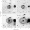 |
Fig. 1 Multi-epoch nebular images of FH Ser. The different panels show NTT SUSI Hα+[N II] (top left), HST WFPC2-PC F656N Hα (top right), VLT VIMOS Hα+[N II] (bottom left), and NOT ALFOSC Hα (bottom right) images. In all panels, north is up and east is to the left. The field of view is the same in all panels, and the origin is defined to be the position of the central star. |
3.2 Hα+[N II] spectral profile
The integrated Hα and [N II] λλ6548,6584 line profiles of the nebular component of FH Ser are shown in Fig. 2. Velocities with respect to the Hα line (λ=6562.849 Å) are referred to the local standard of rest (LSR). The three emission lines overlap notably, with a main double-peak at ≈±300 km s−1, a faint red wing between +800 and +1350 km s−1, and a much fainter blue shoulder3 down to ≈−1050 km s−1.
The emission line profile in Fig. 2 implies a blue edge for the [N II] λ6548 emission line at −375 km s−1 and a red edge for the [N II] λ6584 emission line at +405 km s−1, adopting theoretical wavelengths of λ=6548.05 Å and λ=6583.45 Å for the [N II] λ6548 and [N II] λ6584 emission lines, respectively. Under the reasonable assumption that the two [N II] emission lines have similar line profiles, the Hα line profile is contaminated at velocities ≤−270 km s−1 by the [N II] λ6548 emission line and at velocities ≥+535 km s−1 by the [N II] λ6584 emission line.
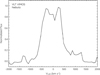 |
Fig. 2 Normalized Hα+[N II] λλ6548,6584 line profile of the integrated nebular emission of FH Ser extracted from the VLT VIMOS observations. |
3.3 Hα and [N II] channel maps
The Hα and [N II] λλ6548,6584 line profiles of the nebular components of FH Ser in Fig. 2 were used to extract the channel maps shown in Fig. 3. Each channel map has a velocity width of 82 km s−1 , corresponding to three spectral channels of 0.6 Å at the wavelength of Hα. The central velocity of each channel in the LSR is labeled for the Hα (white), [N II] λ6548 (cyan), and [N II] λ6584 (red) emission lines.
As noted above, the Hα and [N II] λ6548 emission lines overlap blueward of VHα ≤ −270 km s−1, although [N II] λ6548 is much fainter than Hα. Similarly, the Hα and [N II] λ6584 emission lines overlap redward of VHα ≥ +535 km s−1. Considering the contamination of the [N II] emission lines by Hα, the latter is shown to extend approximately from channels centered at VHα = −632 km s−1 up to VHα = +555 km s−1. The average at ≈−40 km s−1 is consistent with the systemic velocity of −45 km s−1 reported by Gill & O’Brien (2000), whereas the maximum line-of-sight velocity ≈590 km s−1 is about 60 km s−1 higher than their 530 km s−1 estimate.
4 Results
The channel maps shown in Fig. 3 probe different velocity layers of the nova shell, and they thus provide a tomographic view (e.g. QU Vul; Santamaría et al. 2022). The maps probing the Hα emission line are indicative of an expanding shell; the angular size is maximum at the systemic velocity channel (between −85 and 0 km s−1) and then decreases at higher approaching and receding radial velocities. The channel maps probing the [N II] λ6584 emission line follow a different pattern; the angular size is basically the same in the radial velocity range from −200 to +160 km s−1. The different structures traced by the Hα and [N II] λ6584 emission lines are discussed below using different analysis techniques.
4.1 Hα line maps of the ellipsoidal shell
The Hα line profile at each spaxel of the VLT VIMOS HR orange data cube line maps was fit with multiple Gaussian profiles. After a preliminary inspection of the spectra with the Qfitsview tool4, two narrow components were used for the nebular shell to account for its receding and approaching sides, whereas one additional broad component was required at the location of the central star. Single-peaked broad Balmer emission lines are typical of CVs in high state (e.g., Honeycutt et al. 1986; Dhillon et al. 1991) and can generally be attributed to the effects of disk winds (Murray & Chiang 1996). The wavelength range for the line peak of each component was limited up to 20 Å from the blue and red nebular components to the rest frame, and a narrower range in wavelength of 10 Å centered at the systemic wavelength was set for the stellar component. The line width of each nebular component was set to be larger than 4 Å, but larger than 9 Å for the stellar component. The best-fit parameters of each Gaussian were obtained by applying a Levenberg–Marquardt least-squares fitting using an IDL-based routine. Examples of these fits are shown in Figure 4.
The Gaussian fits to the nebular Hα emission line allowed us to map the radial velocity, velocity dispersion σ, and flux in the receding and approaching sides of the nebular shell of FH Ser (Fig. 5). These are clearly resolved within the shell (Fig. 4 middle), but are blended at its edge (Fig. 4-right). Hα emission is found up to 6″ from the central star of FH Ser. The [N II] λ6584 emission line is detected in some spaxels (as in the spaxel shown in the middle panel of Fig. 4), but not all (as in the spaxel shown in the right panel of Fig. 4).
The receding component is brighter toward PA~210°, while the approaching component surface brightness peaks toward PA~60° The addition of the two components (see the bottom left panel of Fig. 1) is consistent with a limb-brightened shell morphology. The two components show granularity in the flux maps (Fig. 5 right), with clumps seen at different spatial locations. The blue nebular component (Fig. 5, top right) shows two ≃1″ bright clumps toward the north and northeast, and a fainter clump toward the south, whereas the red nebular component (Fig. 5, bottom right) presents two clumpy arcs towards the northeast and southwest.
The narrow nebular components reach velocities of ±550 km s−1 and have a similar velocity dispersion within a radius of 3″ of the central star of σ ≃ 90 km s−1 (or FWHM ≃210 km s−1). Since the spectral resolution is ≃100 km s−1 in FWHM, the line width is notably larger than the spectral resolution. The line width increases at the edge of FH Ser, which can be expected for a thin shell as the line of sight crosses a thicker fraction of the shell at this location, but it can also be expected due to the problematic two-Gaussian fit of components that are too close in velocity. The red component shows a notorious σ enhancement toward the southwest and reaches values of σ up to 200 km s−1.
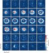 |
Fig. 3 VLT VIMOS tomography of the Hα and [N II] λλ6548,6584 emission lines of FH Ser. Each velocity channel has a width of 82 km s−1, i.e., three spectral channels. The white, cyan, and red labels correspond to LSR velocities of the Hα, [N II] λ6548, and [N II] λ6584 emission lines, respectively. The location of the central star is marked by a red plus sign that serves as a fiducial point in all channel maps. In all maps, north is up and east is to the left. See the text for further details of the spectral and spatial extent of each emission line. |
4.2 3D visualization of the nova remnant of FH Ser
The 3D physical structure of FH Ser is clearly revealed in the Hα+[N II] λλ6548,6584 position-position-velocity (PPV) diagrams shown in Fig. 6, which were computed from the VLT VIMOS channel maps in Fig. 3 using customized Python routines. Three different 3D views of the Hα and [N II] λλ6548,6584 emission lines are shown along the line of sight on the α−δ plane of the sky (i.e., a direct image), and the δ−λ and α−λ planes. In these 3D visualizations, the [N II] λ6584 emission line is seen as the red extension of the Hα line, whereas the [N II] λ6548 emission line is barely seen as a dark blue extension.
The 3D visualizations of the Hα line in the middle and bottom rows of Fig. 6 confirm that its physical structure can be described by a prolate thin ellipsoid, with the expected spatio-kinematic behavior (left panels) and limb-brightness morphology (right panels). This shell morphology is also seen in the [N II] λ6584 emission line as the weak outermost emission in the bottom panels of Fig. 6, particularly in the right panel. The main spatio-kinematic structure revealed by the 3D visualizations of the [N II] λ6584 emission line is, however, very different compared to that of Hα. Instead of an ellipsoid, the [N II] emission is consistent with a tilted ring seen pole-on in the middle panels of Fig. 6 and sideways in the bottom panels of Fig. 6. The bottom right panel of Fig. 6 is suggestive of a similar structure in the Hα line, but it is much fainter than the Hα shell.
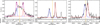 |
Fig. 4 Examples of emission line spectra from the VIMOS cube (black line) and their multi-Gaussian fit (color lines) for the position of the central star (left panel), shell interior (middle panel), and shell edge (right panel). The blue and red Gaussian curves correspond to the two nebular components, and the green curve in the left panel represents a broad stellar component. The residuals from the fit are shown below each panel. As a reference, the vertical solid yellow line in all panels marks the systemic wavelength of Hα. |
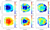 |
Fig. 5 Hα velocity (left), velocity dispersion σ (middle), and flux intensity (right) emission line maps of FH Ser obtained from the multiGaussian fit of individual spaxels in the VLT VIMOS HR orange data cube. The top and bottom panels show the blue and red nebular components, respectively. The cross sign marks the position of the central star (0,0), which is spatially unresolved in the VIMOS data. In all maps, north is up and east is to the left. |
4.3 3D physical structure of the nova remnant of FH Ser
The Hα channel maps in Fig. 3, expansion velocity maps in Fig. 5, and 3D visualizations in Fig. 6 indicate that the Hα- emitting material in FH Ser can mostly be described as a tilted prolate ellipsoidal shell. When we further assume that its expansion is homologous, that is, that the expansion velocity at the location of the shell is radial and proportional to the shell radius at this point, then the observed morphology and kinematics of the nova remnant depend on only a few parameters. A homologous expansion is actually supported by the constant angular expansion of the remnant in time (Santamaría et al. 2020).
Appendix A describes the use of a number of spatio- kinematic measurables, including the age and Hα radius of 4.3 arcsec along the minor axis of FH Ser in the VLT VIMOS images, and the maximum systemic radial expansion velocity and the radius of the location where this maximum velocity is found to constrain the 3D physical structure of this expanding tilted prolate ellipsoid. Appendix A shows that FH Ser can be described as an expanding tilted prolate ellipsoid with an ellipticity e = 1.22 ± 0.03, an equatorial and polar expansion velocity 504±27 km s-1 and 612±35 km s−1, and an inclination of its major axis to the line of sight i = 52° ± 7° at a distance 950 ± 50 pc.
Appendix B goes further and fits the Hα velocity and velocity dispersion 2D maps in Fig. 5 with a similar tilted prolate ellipsoid that expands homologously, but this time, the shell thickness is also considered. This method provides rather consistent values of the equatorial and polar expansion velocity 507 ± 12 km s−1 and 650 ± 15 km s−1, and for the major axis inclination i = 52° ± 2°. Otherwise, the axial ratio e = 1.28 ± 0.02 is slightly higher, whereas the equatorial radius Req = 3.9 arcsec is slightly smaller. The distance estimate to FH Ser according to this method is larger,  , than in Appendix A.
For comparison, Gill & O’Brien (2000) concluded that FH Ser could be described by an ellipsoidal shell with an axial ratio 1.3 ± 0.1 tilted by 62° ± 4° to the line of sight. Their inclination and ellipticity or axial ratio are within the ranges of these parameters as derived in Appendices A and B. Otherwise, the Gaia DR3 parallax distance ( ; Bailer-Jones et al 2021) differs notably from that derived in the first method (950 ± 50 pc), but it is quite similar according to the second method (
 ), which allows us to account for the shell thickness.
The 3D physical structure of the [N II] λ6584 emission line revealed in the 3D visualizations in Fig. 6 is consistent with a ring-like or toroidal structure that is tilted to the line of sight. When this toroidal structure is assumed to be embedded within the ellipsoidal shell, as supported by their similar spatial extent, the same equatorial expansion velocity of ≈505 km s−1 can be adopted. Then the observed maximum expansion velocity ≈±435 km s−1 at the tips of the toroidal structure implies that it is tilted by ≃49° to the plane of the sky, which is consistent with the tilt of the ellipsoidal shell. The [N II] toroidal structure thus forms a belt at the equator of the Hα ellipsoidal shell.
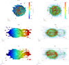 |
Fig. 6 Hα+[NII] emission velocity-colored (left) and intensity (right) position–position–velocity (PPV) diagrams of FH Ser. The top row shows the projection along the observer’s point of view (i.e., the direct image), and the middle and bottom rows show the δ − λ and α − λ projections from the plane of the sky along the east-west and north-south directions, respectively. Information on the LSR radial velocity of Hα is provided by the rainbow color-code shown in the top left panel, with the color span covering the Hα and [N II] λ6584 emission lines of FH Ser. The color-code of the right panels corresponds to normalized flux. |
4.4 Ionized mass and its kinetic energy
The ionized mass Mion of FH Ser can be derived from its intrinsic Hα flux as (see Boyarchuk et al. 1968)
 (1)
(1)
where µ is the mean molecular weight, which can be assumed to be 1.44 for a He/H solar ratio, mp is the proton mass, Np is the proton density, V is the emitting volume, and ε is the filling factor, which can be described as ε = a × b, where a and b are the macroscopic and microscopic filling factor components, respectively (see details in Santamaría et al. 2022). This can be expressed as
 (2)
(2)
where d is the distance to FH Ser, FHα is the unabsorbed (intrinsic) Hα flux, and jHα is the emission coefficient of the Hα line with a value of 4 × 10⁻²⁵ erg cm−3 s−1 (Osterbrock & Ferland 2006). Similarly, the root mean square (rms) density ne can be expressed as
 (3)
(3)
The total observed Hα flux derived from the VLT VIMOS IFS observations is 2.7 × 10⁻¹⁴ erg cm−2 s−1. The extinction toward FH Ser can be estimated using the reddening versus distance curve along its direction as provided by Bayestar195 (Green et al. 2018). At the Gaia distance of 1080 pc for FH Ser, the extinction is quite flat, with E(𝑔 − r) = 0.53 ± 0.01 mag in the distance range from 730 to 1440 pc. The conversion from E(𝑔 − r) to E(B − V) provided by Schlafly & Finkbeiner (2011) implies c(Hβ)=0.77 or E(B − V) = 0.54 mag. After we applied the extinction correction, the intrinsic Hα flux was estimated to be FHα =8.8×10⁻¹⁴ erg cm−2 s−1. This resulted in a total ionized mass Mion = 4.6 × 10⁻⁴ × ε1/2 M⊙ and an rms electron density ne of ≃240 ×ε−1/2 cm−3.
The IFS observations allowed us the opportunity to evaluate the ionized mass in each volume element of the 3D data cube when the velocity (or wavelength) along the ɀ-axis was converted into depth in the physical scale (centimeter, parsec, or arcsecond). In this way, the information on the true 3D structure and the inhomogeneous clumpy distribution of the ejected material in the nebular shell can be taken into account, which reduces the uncertainty on the filling factor ε by removing its macroscopic term a. The equatorial expansion velocity of FH Ser is ≃505 km s−1, which corresponds to an equatorial radius of 4.3 arcsec, or ≃7 × 1016 cm at the Gaia DR3 distance of 1080 pc. Thus, the scaling factor between velocity and linear radius
 (4)
(4)
implies that the spectral dispersion of 0.6 Å pix−1 (or 27.4 km s−1 pix−1 at Hα) and the plate scale of 0.66 × 0.66 arcsec2 pix−1 corresponds to a volume element of the 3D data cube of ≃4.3 × 1047 cm3.
The total mass of the nebula as estimated for each volume element of the data cube and these elements added together is 2.6 × 10⁻⁴ × b1/2 M⊙. A comparison of this mass and the mass derived from the total Hα flux computed above implies a value of 0.7 for a, the macroscopic component of the filling factor.
The total volume occupied by the nova shell implies a swept- up mass of 2.4 × 10⁻⁶ M⊙ for an assumed value of 1 cm−1 for the density of the circumstellar medium. The mass of the nova ejecta is thus much greater than the mass of the swept ISM, which it exceeds by a factor 188 × b1/2. This is fully consistent with a free expansion phase, as confirmed by the constant angular expansion of the shell. This is also supported by the kinetic energy of FHSer, Ekin = 1.6 × 1045 erg that was derived by adopting an expansion velocity weighted between the radial velocity and the velocity on the plane of the sky.
5 Discussion
The IFS observations of the nova remnant FH Ser presented here disclose two distinct structural components: a prolate ellipsoidal shell that is most prominent in Hα (and very weak in [N II]), and an equatorial belt that is best seen in [N II] (and probably also present in Hα). The earliest evidence of these structures was presented by Hutchings (1972), who modeled the Hδ line profile using a spherically symmetric shell and a polar-cap shell. A similar investigation on the early development of asymmetries in its ejecta was carried out by Seaquist & Palimaka (1977) based on radio observations.
A growing number of nova remnants displays different large-scale structural components that are distinctly revealed in H I Balmer emission lines and in the forbidden [N II] and [O III] emission lines, such as, HR Del (Harman & O’Brien 2003; Moraes & Diaz 2009), Sab 142 (a.k.a. IPHASXJ210204.7+471015, Guerrero et al. 2018), TPyx (Izzo et al. 2024; Santamaría et al. 2024), and RR Pic (Celedón et al. 2024). These different structural components most likely inform us about chemical or density inhomogeneities or varying excitation conditions in the nova ejecta that formed either during the TNR, or that resulted from the interaction of the nova ejecta with the accretion disk and donor companion (Drake & Orlando 2010). These are quite notorious in early near-IR IFS observations of nova remnants (e.g., V723 Cas, a.ka.a. Nova Cas 1995, and V5668 Sgr, a.k.a. Nova Sgr 2015b; Lyke & Campbell 2009; Takeda et al. 2022). The rather similar inclination of the symmetry axes of the two structures with respect to the line of sight in FH Ser suggests that they both formed as the result of the same shaping process. The most likely explanation is that the nova ejecta interacted with the accretion disk around the WD6, which strips material from the disk that is not completely disrupted, and this mass-loads the ejecta preferentially along the plane of the accretion disk (Booth et al. 2016; Figueira et al. 2018), which slows it down. The interaction of these ejecta with the subsequent fast stellar wind from the WD results in the ellipsoidal shell morphology (e.g., Orlando et al. 2017), as the latter encounters a higher density and more slowly expanding material along the accretion disk plane. The mass-loading of the ejecta is also supported by the ionized mass of FH Ser, which is far higher than the theoretical predictions for a nova outburst with a similar expansion velocity and decline time (Yaron et al. 2005).
Celedón et al. (2024) argued that equatorial structures that are most prominent in forbidden lines have to be associated with the lower-density material of evolved old nova remnants, but the young age of FH Ser (39.37 yrs at the time of the VLT VIMOS observations) contradicts this. It is more likely that the interaction of the ejecta with the accretion disk enhances shocks that amplify the emission in shock-sensitive emission lines, such those of [N II]. This is also the case of Sab 142 (Guerrero et al. 2018), where the H I Balmer lines are not even detected in the equatorial ejecta, in contrast to T Pyx (Izzo et al. 2024; Santamaría et al. 2024), where the equatorial ring-like structure is most prominent in the H I Balmer lines. These differences highlight the diversity of nova remnants and their complex shapes.
Narrow-band Hα and [N II] images of nova remnants might be contaminated by the image of the other emission line, given their high expansion velocities. This is an important issue particularly for nova remnants for which different structural components are traced by the Hα and [N II] emissions. Thus, structural features associated with one emission line may be detected in the narrow-band image of the other emission line. The HST WFPC2 F656N filter we used to obtain the image shown in the top right panel of Fig. 1 has a pivotal wavelength of 6563.81 Å and an FWHM of 28.55 Å, which results in a non-negligible sensitivity to the total emission of the [N II] λλ6548,6584 emission lines. It is thus very likely that the equatorial ring in this image includes a significant contribution of [N II] emission. The images of HR Del (Harman & O’Brien 2003) and TPyx (Izzo et al. 2024; Santamaría et al. 2024) are most likely also affected by this issue. This emphasizes the advantages (even the need) of using IFS observations instead of direct imaging in order to reveal the true morphology and physical structure of nova remnants.
The use of IFS observations provides a critical advantage in fitting the geometry and inclination of an ellipsoidal shell with the homologous expansion that describes the nova remnant. Two different methods were developed here to obtain the best-fit parameters of this ellipsoidal shell. One method is presented in Appendix A and uses spatio-kinematic information along the major axis of FH Ser, and the other method is described in Appendix B and uses 2D velocity maps that can be uniquely derived from IFS observations. The two methods provide similar (although not exactly the same) best-fit parameters. One major difference results for the expansion distance to FH Ser, which is discrepant with respect to the Gaia DR3 parallax distance ( ; Bailer-Jones et al 2021) in the first method, but it is quite similar according to the second method, which allows us to account for the shell thickness. It is well known that the Gaia determination of parallax distances to nova remnants results in notably different distances than those derived from their nebular expansion, in particular, for sources farther away than 1.0 kpc (Schaefer 2018; Della Valle & Izzo 2020). This discrepancy can be attributed to the methods used to derive distances from the Gaia parallax, as discussed in length by Selvelli & Gilmozzi (2019) and Tappert et al. (2020), but also to difficulties in the expansion distance method for barely resolved nova remnants (Downes & Duerbeck 2000) or by its application to expanding prolate ellisoidal shells (Wade et al. 2000). The method described in Appendix B shows that the consideration of the shell thickness in the determination of the expansion distance fixes the problem of a discrepant Gaia distance for FH Ser. We have started a large program to fit available IFS observations of nova remnants using the full potential of these spatio-kinematic data, in conjunction with available narrowband images to further use their spatial information to better constrain the models.
6 Conclusions
The source FH Ser is a slow classical nova that experienced a nova outburst in February 1970. Its nova remnant is elliptical and has multiple knots. A peculiar ring-like filament lies along its minor axis. We used integral field spectroscopic VLT VIMOS observations with a spectral resolution R ~ 3000 of the nebular remnant of FH Ser to investigate its spatio-kinematic structure in the Hα and [N II] 6548,6584 emission lines.
The data cube was analyzed using position-position-velocity (PPV) diagrams of its velocity field and emission intensity. The 3D visualizations of FH Ser uniquely reveal two different structural components: a tilted prolate ellipsoidal shell that is most prominent in Hα, and a ring-like structure that is most prominent in the forbidden emission line of [N II]. The best Hα narrow-band images of FH Ser mix the Hα emission of the outer elliptical envelope and the [N II] emission of knotty and filamentary inner ring-like structure.
The spatio-kinematics of the Hα emission was modeled by adopting a prolate ellipsoidal shell model with a homologous expansion. The data were fit using two different techniques to determine the inclination, axial ratio, and the polar and equatorial velocity of this prolate ellipsoid. The first technique used a number of particular measurables of a tilted expanding ellipsoid to derive these parameters, and the second technique took full advantage of the integral field spectroscopic observations to model the 2D velocity maps using a Markov chain Monte Carlo fit. The two fits imply an inclination of the major axis of the ellipsoid of ≈52° to the line of sight, a major-to-minor axis ratio of ≈1.25, and an equatorial velocity of ≈505 km s−1. The relatively slow expansion velocity and high axis ratio agrees with the classification of FH Ser as a slow nova.
The [N II]-dominated ring-like structure has the same inclination angle as the Hα-dominated ellipsoidal shell. It can thus be described as an equatorial belt-like structure of the ellipsoidal shell that can be linked to the process that shaped the latter. The most likely connection is the interaction of the nova ejecta with the accretion disk around the WD at the time of the nova outburst. Stripped material from the accretion disk is proposed to mass-load the nova ejecta, which slows it down on the equatorial plane.
The 3D structure of FH Ser was used to refine the estimate of its ionized mass, which was found to be Mion = 2.6 × 10⁻⁴ M⊙. The ionized mass is much higher than the interstellar medium that is swept up by the nova shell, which conforms with its free expansion and high kinetic energy of 1.6 × 1045 erg. It is also much higher than the theoretical expectations for the ejecta of a slow nova, which confirms the mass-loading of the nova ejecta.
We demonstrated that integral field spectroscopy at a dispersion R ≳ 3000 provides suitable means to separate different structural components of nova remnants, to derive reliable estimates of key parameters, such as the shell aspect ratio, its ionized mass, and expansion distance, and to spatio-kinematically resolve small-scale structures (clumping). New methods for analyzing the rich data cube provided by integral field spectroscopic observations of the complex nova remnants are being developed for these purposes.
Acknowledgements
M.A.G. and S.C. acknowledge financial support from grant CEX2021-001131-S funded by MCIN/AEI/10.13039/501100011033. M.A.G. also acknowledges financial support from grant PID2022-142925NB-I00 from the Spanish Ministerio de Ciencia, Innovación y Universidades (MCIU) cofunded with FEDER funds. E.S. thanks UNAM DGAPA for a postdoctoral fellowship. J.A.T. and E.S. acknowledges support from the UNAM PAPIIT project IN 102324. This work has made extensive use of NASA’s Astrophysics Data System (ADS). A.E. acknowledges the financial support from the Spanish Ministry of Science and Innovation and the European Union – NextGenerationEU through the Recovery and Resilience Facility project ICTS-MRR-2021-03-CEFCA.
Appendix A One-dimensional analytical fit of a homologous expanding prolate ellipsoidal shell
The observed morphology and kinematics of the nova remnant of FH Ser, on the assumption that it can be described by a tilted prolate ellipsoidal shell with homologous expansion, depend only on a few parameters, namely (1) the shell aspect ratio e between the semi-major axis a and the semi-minor axis b,
 (A.1)
(A.1)
(2) the inclination of the major-axis with the line of sight i, (3) the distance d, (4) the semi-minor axis b, and (5) the remnant age ∆t. The latter two parameters can be fixed to the time of the VLT VIMOS observations (i.e., b = 4.3 arcsec and ∆t = 39.37 yr).
Other key parameters, such as the equatorial and polar expansion velocities, Veq and Vp , respectively, can be simply expressed in terms of the distance and aspect ratio, given the known remnant age and semi-minor axis, as
 (A.2)
(A.2)
which is just another way of writing the angular expansion along the minor axis derived by Santamaría et al. (2020) of  yr−1, and
 (A.3)
(A.3)
A.1 Special measurables of a tilted expanding ellipsoid
Let’s consider Figure A.1 as a description of the slice of an ellipsoid along its projected major axis. There are a number of spatio-kinematic measurables in a tilted expanding ellipsoid that can be used to determine the unknown parameters e, i, and d. The relationships between these spatio-kinematic measurables and the unknown parameters are described next.
A.1.1 Projected semi-major axis
The Cartesian coordinates of the ellipse representative of the slice along the major axis of an ellipsoid with semi-minor axis b and aspect ratio e can be written as
 (A.4)
(A.4)
which is the thin ellipse shown in Figure A.1, where r is the distance on the plane of the sky to the center, z is the distance to the plane of the sky, and ϕ is the angle with the semi-major axis, which varies from 0° to 360°. Considering an inclination angle of the major-axis with respect to the line of sight i, then the value b = 4.3 arcsec and the relationship e = a/b can be used to derive the projected radius of a point on this tilted ellipse
 (A.5)
(A.5)
and its distance to the plane of the sky
 (A.6)
(A.6)
This tilted ellipse is shown in Figure A.1 by a thick ellipse, where the grey dots around it remind us that the observed remnant shell is not infinitely thin, but a distribution of emitting volumes distributed within a relatively thin shell.
At the maximum projected distance
 (A.7)
(A.7)
Expressing cos ϕ and sin ϕ as a function of tan i, it can be shown that
 (A.8)
(A.8)

for ϕ at the maximum radial projection on the sky. The value of rmax is estimated to be 4.9 arcsec, thus the projected (observed) axial ratio is ≃1.14 ± 0.03, adopting an uncertainty of 0.1 arcsec for rmax and b.
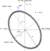 |
Fig. A.1 Sketch of a slice of the ellipsoidal shell model across the plane including its major axis and tilt direction. The geometry of the ellipsoid is defined by the semi-major axis a, semi-minor axis b, their ratio e, and the inclination angle i with the line of sight, illustrated on the sketch. The singular measurables projected semi-major axis rmax, maximum systemic radial velocity |


Figure A.2 shows the variation of the observed axial ratio with the inclination angle for 5 different values of the true ellipticity. As expected, the observed axial ratio increases with the true axial ratio and the tilt of the major axis with the line of sight.
A.1.2 Maximum systemic radial velocity
The systemic radial velocity at any point of an ellipsoid with homologous expansion is proportional to the distance to the plane of the sky z. Thus it can be expressed as
 (A.10)
As in the previous section, the maximum systemic radial velocity can be computed as
 (A.11)
that after expressing cos ϕ and sin ϕ as a function of tan i, results in the following expression
 (A.12)

for ϕ at the maximum systemic radial velocity.
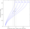 |
Fig. A.2 Variation of the projected semi-major axis of an ellipsoid along its symmetry axis for 5 different values of its ellipticity (labeled in blue) with its major axis inclination. The observed semi-major axis of 4.″9 of FH Ser is marked by a solid vertical line, with 1-σ uncertainty marked by vertical dotted lines. The black dot corresponds to the best fit value, with blue dots in the left and right panels representing acceptable values within the uncertainty of the observed parameters. |
Figure A.3 shows the variation of the ratio of the observed maximum systemic radial velocity and distance with the inclination angle for 5 different values of the true ellipticity. The observed maximum systemic radial velocity is estimated to be 530 ± 10 km s−1, whereas the Gaia distance to FH Ser is  pc. The maximum systemic radial velocity is shown to increase with axial ratio and decrease with increasing tilt of the ellipsoid with the line of sight. We notice that there is marginal agreement between the predicted and expected values of this ratio, suggesting that FH Ser could be located closer than indicated by its Gaia distance. The 2-σ lower uncertainty in the Gaia distance is shown in this plot as an additional vertical dashed line.
A.1.3 Radial distance at maximum systemic radial velocity
The above maximum systemic radial velocity is achieved at a projected radius
 (A.14)
which is plotted in the right panel of Figure A.4 for 5 different values of the true ellipticity. The projected radius of the point with the maximum systemic radial velocity is measured in the velocity maps presented in Figure 5. This results to be 0.92 ± 0.12 arcsec, which is plotted in Figure A.4 as a vertical solid line with 1-σ uncertainty as dotted lines.
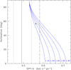 |
Fig. A.3 Variation of the ratio of the maximum systemic radial velocity to the distance of an ellipsoid for 5 different values of its ellipticity (labeled in blue) with its major axis inclination. The ratio between the observed maximum systemic radial velocity of FH Ser and its Gaia distance is marked by a solid vertical line, with 1-σ uncertainty marked by vertical dotted lines and the 2-σ lower uncertainty by a vertical dashed line. The black dot corresponds to the best fit value. |
A.2 Geometry of the nova remnant of FH Ser
Figures A.2, A.3, and A.4 place some constraints on the different parameters e, i, and d. The plots of projected axial ratio (Fig. A.2) and projected point at maximum systemic radial velocity (Fig. A.4) are clearly contrasting. The best joint-fit to both variations is achieved only for a relatively low ellipticity, ≃1. 215, and an intermediate inclination angle, i ≈ 52.2° (black dot in these figures). Accounting for the 1-σ uncertainty, fits can be achieved within e and i ranges 1.189 ≤ e ≤ 1.243 and 45.8° ≤ i ≤ 59.5° (blue dots in these figures). Therefore the values of e and i are estimated to be 1.215±0.027 and 52° ± 7°, respectively.
On the other hand, the ratio of the maximum systemic radial velocity to distance (Fig. A.3) is inconsistent with the geometrical models, unless the distance is notably lower, 950±50 pc, than the Gaia distance of  pc. The equatorial and polar velocity would be 504±27 and 612±35 km s−1, respectively.
Appendix B Two-dimensional Montecarlo model fitting of a homologous expanding prolate ellipsoidal shell
The velocity and velocity dispersion maps (left and middle panels of Fig. 5, respectively) provide means for a robust, 2D fit of the expanding shell of FH Ser. The fits is described below together with the results of these fits.
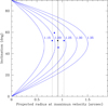 |
Fig. A.4 Variation of the projected radius at the maximum systemic radial velocity for 5 different values of its ellipticity (labeled in blue) with its major axis inclination. The observed projected radius at the maximum systemic radial velocity of FH Ser is marked by a solid vertical line, with 1-σ uncertainty marked by vertical dotted lines. In all panels, the black dot corresponds to the best fit value, with blue dots in the left and right panels representing acceptable values within the uncertainty of the observed parameters. |
B.1 Geometrical model
The same tilted prolate ellipsoidal shell model with homologous expansion (see Fig A.1) is adopted, thus its morphology depends only on two free parameters, (1) the mean equatorial radius Req ∊ ℝ+, which corresponds to the semi-minor axis, b, and (2) the shell aspect ratio e between the semi-major axis, a, and the semi-minor axis, b, i.e, e = a/b ∊ [1, ∞). Unlike in Appendix A, this ellipsoid will be assumed here to have a finite thickness following a normal distribution with standard deviation w from its central value. The value of w has been fixed to 0.13 arcsec, according to the FWHM of 0.31 arcsec of the shell measured in HST images.
The model will additionally have three internal model parameters; the azimuthal angle θ ∈ (−π, π] measured from the x axis (the North direction on the plane of the sky), the polar angle ϕ ∈ [0, π] measured from the z axis (the line of sight), and the depth parameter ξ ∊ [−3, +3] that, for given values of the polar and azimuthal angles, sets the “distance” of a point within the shell from the mean radius along this direction.
The model of a prolate spherical shell is thus described by the following equations
 (B.1)
(B.1)
where (Req + wξ) is the length of the semi-minor axis, which varies from Req − 3w to Req + 3w depending on the value of the model parameter ξ. The general Cartesian form of an ellipsoidal shell is derived from Eq. B.1:
 (B.2)
(B.2)
The infinitely thin prolate ellipsoidal surface of Appendix A would be recovered if the width parameter w value were set to nil.
B.1.1 Tilted model
The inclination of the ellipsoidal shell with the line of sight and North directions require adding two additional free parameters, namely: (3) the inclination of the major-axis with respect to the line of sight, i ∈ [0, π/2], and (4) the position angle, PA∈ [−π, π), which is the rotation angle with respect to the x axis. In order to correctly take into account the effects of these two orientation changes, a rotation along the x axis by i and a rotation along the z axis by PA needs to be applied. This is carried out by the following transformation matrix
![${{\bf{R}}_{\bf{T}}} = \left[ {\matrix{ {\cos (PA)} & {\sin (PA)\cos i} & {\sin (PA)\sin i} \cr { - \sin (PA)} & {\cos (PA)\cos i} & {\cos (PA)\sin i} \cr 0 & { - \sin i} & {\cos i} \cr } } \right]$](/articles/aa/full_html/2025/02/aa52743-24/aa52743-24-eq30.png) (B.3)
(B.3)
So given the position vector P = [x, y, z]T of a point within the spheroidal shell we can obtain the position vector in the observer’s reference system P′ = RTP with z′ going along the line of sight.
B.1.2 Line-of-sight velocity
The information along the z axis (line of sight) derived from the model described above can be compared with the velocity along the line of sight (or simply the radial velocity Vr) and velocity dispersion maps in Fig. 5. As described in Appendix A, there are relationships between Veq and Vp with the distance, ellipticity, angular size along the minor axis, and age of the shell (Eqs. A.2 and A.3).
Given a set of free parameters {Req , e, i, PA} defining the shell geometry and space orientation, the velocity distribution of an homologously expanding shell can be modeled introducing an additional free parameter, (5) the equatorial velocity of the shell7, Veq. In a homologously expanding shell, the velocity at a given point has a radial direction and is proportional to the distance to the center V ∝ P. Thus it can be proven that
 (B.4)
(B.4)
where Veq is taken in the middle of the shell (ξ = 0). In this way the radial velocity Vr is simply the z component of the velocity in the observer’s reference system
![${V_r} = {V^\prime } \cdot {\hat k^\prime } = {{{V_{{\rm{eq}}}}} \over {{R_{{\rm{eq}}}}}}[z\cos i - y\sin i]$](/articles/aa/full_html/2025/02/aa52743-24/aa52743-24-eq32.png) (B.5)
(B.5)
The free parameters of the model will be fitted by comparing the model 2D velocity map predictions with the observed radial velocity maps Vr in Fig. 5. The velocity dispersion maps in Fig. 5 will be used to weight the distance between the synthetic and observed velocity maps at each spaxel.
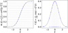 |
Fig. B.1 Distribution of the width modulator ξ for 15 layers. (Left) The solid line corresponds with the normal cumulative distribution function, the dashed lines corresponds with the intervals of equal probability, meanwhile the blue dots corresponds with the intersections of the function with the intervals. (Right) The solid line corresponds with a standard normal distribution, the blue dots are the value of the function evaluated in the intersections of the equally probable intervals, meanwhile the crossed points in the bottom shows qualitatively the separation between the layers in the model with respect to the center of the shell. |
B.1.3 Synthetic observations
Given a set of the free parameters {Req, e, Veq, i, PA], the model parameters {ξ, θ, ϕ} are used to sample points within the spheroidal shell. To represent significantly the model, the layering approach will use a width modulator ξ discretized by means of the normal cumulative distribution function defined as
![$\Phi (x) = {1 \over {\sqrt {2\pi } }}\int_{ - \infty }^x {{e^{ - {{{t^2}} \over 2}}}} dt = {1 \over 2}\left[ {1 + {\mathop{\rm erf}\nolimits} \left( {{x \over {\sqrt 2 }}} \right)} \right]$](/articles/aa/full_html/2025/02/aa52743-24/aa52743-24-eq33.png) (B.6)
(B.6)
being erf(z) the standard error function
 (B.7)
(B.7)
in order to ξ being a normally distributed value as seen in the right panel of Fig. B.1. This is achieved by uniformly splitting the range of the cumulative distribution function (Eq. B.6) into (nlayers − 1) intervals as shown in the left panel of the Fig. B.1 and finding the value of ξ in every intersection. Here nlayers is the number of modeled layers.
Thus for every value of ξi, there is an ellipsoidal surface of semi-minor axis bi = Req + wξi. Since every surface has different area, in order to conserve a point surface density, every layer needs to have a number of points given by relationship
 (B.8)
(B.8)
where  represents the standard floor operation, which rounds down the value inside the brackets to the nearest integer, and 2ni + 1 is the number of points in the i-th layer. The minimum number of points per layer is 2n1 + 1 for a value of i = 1.
Within each layer, the points where uniformly distributed in the surface by means of a Fibonacci lattice, which has a better spatial covering properties than the longitude-latitude lattice (González 2010). To sample the polar and azimuthal angles a variation of the equations shown in González (2010) was used
 (B.9)
(B.9)
where  is the golden ratio. This variation gives for every layer a little offset to both angles in order to prevent the polar under density of points and improve the spatial sampling. In this work we used nlayers = 512 and n1 = 2048 for the fitting.
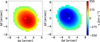 |
Fig. B.2 Example of a synthetic observation produced by the model with the set of parameters Req = 5.″0, w = 0.″13, e = 1.4, Veq = 400 km s−1, i = 45°, PA = 45°. The field of view and spatial resolution are the same as in Fig 5. The center is marked by a white cross. |
Once the model is sampled, 2D histograms of the mean velocity per bin were made as shown in Figure B.2. Those histograms have the same pixel size and spatial resolution as the VLT VIMOS observations to allow a fair comparison of the model with the real data.
B.1.4 Observed data filtering
The 3D visualization of the maps of the red and blue velocity components at the top-panel of Fig. B.3 reveals a number of spaxels along the outer edge whose behavior differ notably from that expected for an expanding ellipsoidal shell. Velocity excursions and a “kind of swimming ring” at the ellipsoid equator are obvious in this figure. This effect is caused by the problematic two Gaussian fit to the velocity profile at the edge of the shell, where the red and blue velocity components blend together. In addition, the red component showed a hump-like feature at its maximum radial velocity. This is actually caused by contamination from the [N II] ring-like structure (see the middle and bottom panels of Fig. 6).
The velocity dispersion maps were used to downplay these effects by giving a lower weight in the fit to spaxels with larger velocity dispersion, but the effects of these spaxels on the fit were still noticeable. In order to definitely alleviate the impact of these spaxels, they were disregarded in the fit using the mask shown in the middle-panel of Fig. B.3. Similarly, since the velocity information of the spaxels affected by the contamination from the [N II] ring-like structure do not fully represent that of the expanding ellipsoid, these spaxels have also been disregarded for the fit. The 3D visualization of the useful maps of the red and blue velocity components is shown at the bottom-panel of Fig. B.3.
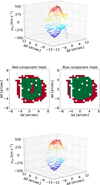 |
Fig. B.3 (top) 3D scatter plot of the velocity observations. The spax- els along the edge of the shell shows noticeable excursions in velocity, as well as a "swimming ring-like" feature. (middle) Pixels used in the MCMC procedure (green) and those masked out (red) because the derived value of Vlos differs notably for an expanding spheroidal shell. The center used is located at position (0,0) as marked with a white cross. (bottom) 3D scatter plot of the velocity observations once the mask is applied (grey dots). The remaining data points resemble a spheroidal- like structure. |
B.2 Markov Chain Montecarlo fit
In order to fit a homologous expanding prolate ellipsoidal shell model, a MCMC (Markov Chain Montecarlo) approach was implemented using the Python library emcee (Foreman-Mackey et al. 2013). The details of this procedure are explained below.
B.2.1 Likelihood function
The comparison of the synthetic blue and red components of the radial expansion velocity with the observed ones in Fig. 5 was made on a pixel-by-pixel basis. In this way the likelihood function is defined as
![$\ln p\left( {\v \mid {R_{{\rm{eq}}}},w,,{V_{{\rm{eq}}}},i,PA} \right) = - {1 \over 2}\sum\limits_i {\left[ {{{{{\left( {{\v _i} - \v _i^\prime } \right)}^2}} \over {s_i^2}} + \ln \left( {2\pi s_i^2} \right)} \right]} {\rm{, }}$](/articles/aa/full_html/2025/02/aa52743-24/aa52743-24-eq39.png) (B.10)
(B.10)
where i represents a pixel and υi, si and υ′i correspond to the observed velocity, observed velocity dispersion, and model predicted velocity in pixel i, respectively. The addition on the right term of this equation over all pixels is made considering simultaneously the red and blue velocity components. It must be remarked that only valid pixels, as masked according to Fig. B.3, are considered here.
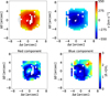 |
Fig. B.4 (top) MCMC best-fit model for the red (left) and blue (right) velocity components of the expanding ellipsoid shown as contours overimposed on the observed velocity maps shown in Fig. 5, and (bottom) absolute differences between the MCMC best-fit model and the velocity maps in Fig. 5 with respect to each image pixel velocity dispersion. The center is located at position (0,0) as marked with a white cross. |
B.2.2 Parameter’s space
The prior distribution for every parameter is adopted to be flat (uninformed prior distribution), since there is no initial information about them. Otherwise every parameter has its respective domain, but a feasible fit of the observations via MCMC requires making a good guess of them. The observed distribution’s edge of the shell seems to be around 5 arcsec (Fig. 5), thus it has been constrained to be Req ∊ [4″, 6″]. Meanwhile the shell width w was fixed at a value of 0.13 arcsec, as described above. The axial ratio e was constrained to be greater than 1; e ∊ [1, ∞), whereas for the inclination and position angles, all their physical range were taken into account, i.e., i ∊ [0, π/2] and PA ∊ [−π, π). Finally the equatorial velocity can be expected to be in the range Veq = 300 – 600 km s−1.
In order to fit the model to the observations a set of 128 random walkers were initialized based on a uniform probability distribution of the parameter’s ranges described before. We note that an additional constraint was applied to the possible values of e, i, and Req , so that the projected axial ratio was in the range from 1.1 to 1.2, in agreement with the observed axial ratio of the nova remnant measured in the HST image.
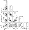 |
Fig. B.5 Corner plot for the resulting parameters of the MCMC approach fitted to the observations. Only the parameter’s space corresponding to 3σ is used in the histograms. |
B.3 Best-fit model
The MCMC best-fit model and the associated difference between the red and blue velocity components are shown in Fig. B.4. The bottom panels of that figure clearly show that the differences between the expected model velocities at each pixel and those actually observed differ by less than the velocity dispersion for most pixels.
The corner plot with the distribution of the best-fit parameters is shown in Fig. B.5. Their best values and 1-σ uncertainties are labeled on top of each row. Some parameters, namely e, Veq and i, exhibit some correlation, which can be expected. The other parameter combinations seem rather uncorrelated.
The best-fit parameters imply equatorial radius and velocity of 3.87±0.01 arcsec and 507±12 km s−1, respectively. The axial ratio is found to be 1.28±0.02, whereas the inclination is 52°±2°. The polar velocity would then be 649±26 km s−1. These best-fit parameters are within 1-σ of those derived in Appendix A, but for the axial ratio, which is a bit larger, 1.28 ±0.02 against 1.22±0.03, but still marginally consistent. Finally it must be noted that the best-fit value of the PA, 81.7°±0.2°, differs with respect to the PA of the shell of 86° described in Section 2.3.1, which reflects the limited spatial information of the velocity maps used to constrain the fit.
The information on Req and Veq provides a distribution for the distance (Fig. B.6), which is found to be 1064±26 pc, in agreement with the Gaia estimate of  pc.
pc.
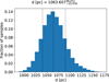 |
Fig. B.6 Distribution of the derived distances using the corresponding velocity distribution from MCMC. Calculated using Req and Veq from the MCMC fit. |
References
- Andersen, P. H., Borra, E. F., & Dubas, O. V. 1971, PASP, 83, 5 [Google Scholar]
- Bailer-Jones, C. A. L., Rybizki, J., Fouesneau, M., et al. 2021, AJ, 161, 147 [NASA ADS] [CrossRef] [Google Scholar]
- Bode, M. F., & Evans, A. 2012, Classical Novae (Cambridge University Press) [Google Scholar]
- Borra, E. F., & Andersen, P. H. 1970, PASP, 82, 1070 [NASA ADS] [CrossRef] [Google Scholar]
- Booth, R. A., Mohamed, S., & Podsiadlowski, P. 2016, MNRAS, 457, 822 [NASA ADS] [CrossRef] [Google Scholar]
- Boyarchuk, A. A., Gershberg, R. E., Godovnikov, N. V., et al. 1968, Planet. Nebulae, 34, 162 [NASA ADS] [CrossRef] [Google Scholar]
- Burkhead, M. S., & Seeds, M. A. 1970, ApJ, 160, L51 [NASA ADS] [CrossRef] [Google Scholar]
- Burkhead, M. S., Penhallow, W. S., Honeycutt, R. K. 1971, PASP, 83, 338 [CrossRef] [Google Scholar]
- Casanova, J., José J., & Shore, S. N. 2018, A&A, 619, A121 [NASA ADS] [CrossRef] [EDP Sciences] [Google Scholar]
- Celedón, L., Schmidtobreick, L., Tappert, C., et al. 2024, A&A, 681, A106 [NASA ADS] [CrossRef] [EDP Sciences] [Google Scholar]
- Chesneau, O., Banerjee, D. P. K., Millour, F., et al. 2008, A&A, 487, 223 [NASA ADS] [CrossRef] [EDP Sciences] [Google Scholar]
- Della Valle, M., & Izzo, L. 2020, A&A Rev., 28, 3 [NASA ADS] [CrossRef] [Google Scholar]
- della Valle, M., Gilmozzi, R., Bianchini, A., & Esenoglu, H. 1997, A&A, 325, 1151 [Google Scholar]
- Dhillon, V. S., Marsh, T. R., & Jones, D. H. P. 1991, MNRAS, 252, 342 [NASA ADS] [CrossRef] [Google Scholar]
- Downes, R. A., & Duerbeck, H. W. 2000, AJ, 120, 2007 [NASA ADS] [CrossRef] [Google Scholar]
- Drake, J. J., & Orlando, S. 2010, ApJ, 720, L195 [NASA ADS] [CrossRef] [Google Scholar]
- Duerbeck, H. W. 1992, AcA, 42, 85 [Google Scholar]
- Evans, A., Tyne, V. H., Smith, O., et al. 2005, MNRAS, 360, 1483 [NASA ADS] [CrossRef] [Google Scholar]
- Figueira, J., José, J., García-Berro, E., et al. 2018, A&A, 613, A8 [NASA ADS] [CrossRef] [EDP Sciences] [Google Scholar]
- Foreman-Mackey, D., Hogg, D. W., Lang, D., Goodman, J. 2013, PASP, 125, 306 [NASA ADS] [CrossRef] [Google Scholar]
- Freudling, W., Romaniello, M., Bramich, D. M., et al. 2013, A&A, 559, A96 [NASA ADS] [CrossRef] [EDP Sciences] [Google Scholar]
- Gallagher, J. S., & Code, A. D. 1974, ApJ, 189, 303 [NASA ADS] [CrossRef] [Google Scholar]
- Gehrz, R. D. 1999, PhR, 311, 405 [Google Scholar]
- Gehrz, R. D., Jones, T. J., Woodward, C. E., et al. 1992, ApJ, 400, 671 [Google Scholar]
- Gill, C. D., & O’Brien, T. J. 2000, MNRAS, 314, 175 [NASA ADS] [CrossRef] [Google Scholar]
- González, Á. 2010, MatGe, 42, 49 [Google Scholar]
- Green, G. M., Schlafly, E. F., Finkbeiner, D., et al. 2018, MNRAS, 478, 651 [Google Scholar]
- Greenhouse, M. A., Grasdalen, G. L., Woodward, C. E., et al. 1990, ApJ, 352, 307 [Google Scholar]
- Guerrero, M. A., Sabin, L., Tovmassian, G., et al. 2018, ApJ, 857, 80 [Google Scholar]
- Hack, M., Selvelli, P., Bianchini, A., & Duerbeck, H. W. 1993, NASSP, 413 [Google Scholar]
- Harman, D. J., & O’Brien, T. J. 2003, MNRAS, 344, 1219 [NASA ADS] [CrossRef] [Google Scholar]
- Hayward, T. L., Saizar, P., Gehrz, R. D., et al. 1996, ApJ, 469, 854 [Google Scholar]
- Hirose, H., & Honda, M., 1970, IAUCirc. 2212 [Google Scholar]
- Honeycutt, R. K., Schlegel, E. M., & Kaitchuck, R. H. 1986, ApJ, 302, 388 [NASA ADS] [CrossRef] [Google Scholar]
- Hutchings, J. B. 1972, MNRAS, 158, 177 [NASA ADS] [CrossRef] [Google Scholar]
- Hyland, A. R., & Neugebauer, G. 1970, ApJ, 160, L177 [NASA ADS] [CrossRef] [Google Scholar]
- Izzo, L., Pasquini, L., Aydi, E., et al. 2024, A&A, 686, A72 [NASA ADS] [CrossRef] [EDP Sciences] [Google Scholar]
- José, J., & Hernanz, M. 1998, ApJ, 494, 680 [Google Scholar]
- Kato, M., & Hachisu, I. 2003, ApJ, 598, L107 [NASA ADS] [CrossRef] [Google Scholar]
- Lyke, J. E., & Campbell, R. D. 2009, AJ, 138, 1090 [NASA ADS] [CrossRef] [Google Scholar]
- Mason, C. G., Gehrz, R. D., Woodward, C. E., et al. 1996, ApJ, 470, 577 [NASA ADS] [CrossRef] [Google Scholar]
- Moraes, M., & Diaz, M. 2009, AJ, 138, 1541 [NASA ADS] [CrossRef] [Google Scholar]
- Murray, N., & Chiang, J. 1996, Nature, 382, 789 [NASA ADS] [CrossRef] [Google Scholar]
- Orlando, S., Drake, J. J., & Miceli, M. 2017, MNRAS, 464, 5003 [CrossRef] [Google Scholar]
- Osterbrock, D. E., & Ferland, G. J. 2006, Astrophysics of Gaseous Nebulae and Active Galactic Nuclei, 2nd edn., (Sausalito, CA: University Science Books) [Google Scholar]
- Patterson, J., Uthas, H., Kemp, J., et al. 2013, MNRAS, 434, 1902 [NASA ADS] [CrossRef] [Google Scholar]
- Rosino, L., Ciatti, F., & della Valle, M. 1986, A&A, 158, 34 [Google Scholar]
- Santamaría, E., Guerrero, M. A., Ramos-Larios, G., et al. 2020, ApJ, 892, 60 [CrossRef] [Google Scholar]
- Santamaría, E., Guerrero, M. A., Toalá, J. A., et al., 2022, MNRAS, 517, 2567 [CrossRef] [Google Scholar]
- Santamaría, E., Toalá, J. A., Guerrero, M. A., et al. 2024, MNRAS, 530, 4531 [CrossRef] [Google Scholar]
- Schaefer, B. E. 2018, MNRAS, 481, 3033 [NASA ADS] [CrossRef] [Google Scholar]
- Schlafly, E. F., & Finkbeiner, D. P. 2011, ApJ, 737, 103 [Google Scholar]
- Seaquist, E. R., & Palimaka, J. 1977, ApJ, 217, 781 [Google Scholar]
- Selvelli, P., & Gilmozzi, R. 2019, A&A, 622, A186 [NASA ADS] [CrossRef] [EDP Sciences] [Google Scholar]
- Shore, S. N. 2013, A&A, 559, L7 [NASA ADS] [CrossRef] [EDP Sciences] [Google Scholar]
- Starrfield, S., Iliadis, C., & Hix, W. R. 2016, PASP, 128, 051001 [Google Scholar]
- Starrfield, S., Bose, M., Iliadis, C., et al. 2020, ApJ, 895, 70 [NASA ADS] [CrossRef] [Google Scholar]
- Takeda, L., Diaz, M., Campbell, R. D., et al. 2022, MNRAS, 511, 1591 [NASA ADS] [CrossRef] [Google Scholar]
- Tappert, C., Vogt, N., Ederoclite, A., et al. 2020, A&A, 641, A122 [NASA ADS] [CrossRef] [EDP Sciences] [Google Scholar]
- Wade, R. A., Harlow, J. J. B., & Ciardullo, R. 2000, PASP, 112, 614 [NASA ADS] [CrossRef] [Google Scholar]
- Yaron, O., Prialnik, D., Shara, M. M., et al. 2005, ApJ, 623, 398 [Google Scholar]
Helium-rich material is also transferred in certain systems (see, e.g., Kato & Hachisu 2003).
Note that the accretion disk is not necessarily coplanar with the orbital plane, but a tilted precessing disk is very frequent in CVs as revealed by superhumps in their light curves (e.g., BK Lyn; Patterson et al. 2013).
Contrary to Appendix A, where the distance was adopted as a free parameter, the equatorial expansion velocity, Veq, is preferred here because its allows a straightforward comparison with the velocity maps.
All Figures
|
Fig. 1 Multi-epoch nebular images of FH Ser. The different panels show NTT SUSI Hα+[N II] (top left), HST WFPC2-PC F656N Hα (top right), VLT VIMOS Hα+[N II] (bottom left), and NOT ALFOSC Hα (bottom right) images. In all panels, north is up and east is to the left. The field of view is the same in all panels, and the origin is defined to be the position of the central star. |
| In the text | |
|
Fig. 2 Normalized Hα+[N II] λλ6548,6584 line profile of the integrated nebular emission of FH Ser extracted from the VLT VIMOS observations. |
| In the text | |
|
Fig. 3 VLT VIMOS tomography of the Hα and [N II] λλ6548,6584 emission lines of FH Ser. Each velocity channel has a width of 82 km s−1, i.e., three spectral channels. The white, cyan, and red labels correspond to LSR velocities of the Hα, [N II] λ6548, and [N II] λ6584 emission lines, respectively. The location of the central star is marked by a red plus sign that serves as a fiducial point in all channel maps. In all maps, north is up and east is to the left. See the text for further details of the spectral and spatial extent of each emission line. |
| In the text | |
|
Fig. 4 Examples of emission line spectra from the VIMOS cube (black line) and their multi-Gaussian fit (color lines) for the position of the central star (left panel), shell interior (middle panel), and shell edge (right panel). The blue and red Gaussian curves correspond to the two nebular components, and the green curve in the left panel represents a broad stellar component. The residuals from the fit are shown below each panel. As a reference, the vertical solid yellow line in all panels marks the systemic wavelength of Hα. |
| In the text | |
|
Fig. 5 Hα velocity (left), velocity dispersion σ (middle), and flux intensity (right) emission line maps of FH Ser obtained from the multiGaussian fit of individual spaxels in the VLT VIMOS HR orange data cube. The top and bottom panels show the blue and red nebular components, respectively. The cross sign marks the position of the central star (0,0), which is spatially unresolved in the VIMOS data. In all maps, north is up and east is to the left. |
| In the text | |
|
Fig. 6 Hα+[NII] emission velocity-colored (left) and intensity (right) position–position–velocity (PPV) diagrams of FH Ser. The top row shows the projection along the observer’s point of view (i.e., the direct image), and the middle and bottom rows show the δ − λ and α − λ projections from the plane of the sky along the east-west and north-south directions, respectively. Information on the LSR radial velocity of Hα is provided by the rainbow color-code shown in the top left panel, with the color span covering the Hα and [N II] λ6584 emission lines of FH Ser. The color-code of the right panels corresponds to normalized flux. |
| In the text | |
|
Fig. A.1 Sketch of a slice of the ellipsoidal shell model across the plane including its major axis and tilt direction. The geometry of the ellipsoid is defined by the semi-major axis a, semi-minor axis b, their ratio e, and the inclination angle i with the line of sight, illustrated on the sketch. The singular measurables projected semi-major axis rmax, maximum systemic radial velocity |
| In the text | |
|
Fig. A.2 Variation of the projected semi-major axis of an ellipsoid along its symmetry axis for 5 different values of its ellipticity (labeled in blue) with its major axis inclination. The observed semi-major axis of 4.″9 of FH Ser is marked by a solid vertical line, with 1-σ uncertainty marked by vertical dotted lines. The black dot corresponds to the best fit value, with blue dots in the left and right panels representing acceptable values within the uncertainty of the observed parameters. |
| In the text | |
|
Fig. A.3 Variation of the ratio of the maximum systemic radial velocity to the distance of an ellipsoid for 5 different values of its ellipticity (labeled in blue) with its major axis inclination. The ratio between the observed maximum systemic radial velocity of FH Ser and its Gaia distance is marked by a solid vertical line, with 1-σ uncertainty marked by vertical dotted lines and the 2-σ lower uncertainty by a vertical dashed line. The black dot corresponds to the best fit value. |
| In the text | |
|
Fig. A.4 Variation of the projected radius at the maximum systemic radial velocity for 5 different values of its ellipticity (labeled in blue) with its major axis inclination. The observed projected radius at the maximum systemic radial velocity of FH Ser is marked by a solid vertical line, with 1-σ uncertainty marked by vertical dotted lines. In all panels, the black dot corresponds to the best fit value, with blue dots in the left and right panels representing acceptable values within the uncertainty of the observed parameters. |
| In the text | |
|
Fig. B.1 Distribution of the width modulator ξ for 15 layers. (Left) The solid line corresponds with the normal cumulative distribution function, the dashed lines corresponds with the intervals of equal probability, meanwhile the blue dots corresponds with the intersections of the function with the intervals. (Right) The solid line corresponds with a standard normal distribution, the blue dots are the value of the function evaluated in the intersections of the equally probable intervals, meanwhile the crossed points in the bottom shows qualitatively the separation between the layers in the model with respect to the center of the shell. |
| In the text | |
|
Fig. B.2 Example of a synthetic observation produced by the model with the set of parameters Req = 5.″0, w = 0.″13, e = 1.4, Veq = 400 km s−1, i = 45°, PA = 45°. The field of view and spatial resolution are the same as in Fig 5. The center is marked by a white cross. |
| In the text | |
|
Fig. B.3 (top) 3D scatter plot of the velocity observations. The spax- els along the edge of the shell shows noticeable excursions in velocity, as well as a "swimming ring-like" feature. (middle) Pixels used in the MCMC procedure (green) and those masked out (red) because the derived value of Vlos differs notably for an expanding spheroidal shell. The center used is located at position (0,0) as marked with a white cross. (bottom) 3D scatter plot of the velocity observations once the mask is applied (grey dots). The remaining data points resemble a spheroidal- like structure. |
| In the text | |
|
Fig. B.4 (top) MCMC best-fit model for the red (left) and blue (right) velocity components of the expanding ellipsoid shown as contours overimposed on the observed velocity maps shown in Fig. 5, and (bottom) absolute differences between the MCMC best-fit model and the velocity maps in Fig. 5 with respect to each image pixel velocity dispersion. The center is located at position (0,0) as marked with a white cross. |
| In the text | |
|
Fig. B.5 Corner plot for the resulting parameters of the MCMC approach fitted to the observations. Only the parameter’s space corresponding to 3σ is used in the histograms. |
| In the text | |
|
Fig. B.6 Distribution of the derived distances using the corresponding velocity distribution from MCMC. Calculated using Req and Veq from the MCMC fit. |
| In the text | |
Current usage metrics show cumulative count of Article Views (full-text article views including HTML views, PDF and ePub downloads, according to the available data) and Abstracts Views on Vision4Press platform.
Data correspond to usage on the plateform after 2015. The current usage metrics is available 48-96 hours after online publication and is updated daily on week days.
Initial download of the metrics may take a while.