| Issue |
A&A
Volume 693, January 2025
|
|
|---|---|---|
| Article Number | A321 | |
| Number of page(s) | 21 | |
| Section | Extragalactic astronomy | |
| DOI | https://doi.org/10.1051/0004-6361/202452437 | |
| Published online | 30 January 2025 | |
MICONIC: Dual active galactic nuclei, star formation, and ionised gas outflows in NGC 6240 seen with MIRI/JWST
1
Centro de Astrobiología (CAB) CSIC-INTA, Camino Bajo del Castillo s/n, 28692 Villanueva de la Cañada, Madrid, Spain
2
Telespazio UK for the European Space Agency (ESA), ESAC, Camino Bajo del Castillo s/n, 28692 Villanueva de la Cañada, Spain
3
Sorbonne Université, CNRS, UMR 7095, Institut d’Astrophysique de Paris, 98bis Bd Arago, 75014 Paris, France
4
Institut Universitaire de France, Ministère de l’Enseignement Supérieur et de la Recherche, 1 Rue Descartes, 75231 Paris Cedex 05, France
5
Sterrenkundig Observatorium, Universiteit Gent, Krijgslaan 281 S9, B-9000 Gent, Belgium
6
Leiden Observatory, Leiden University, PO Box 9513 2300 RA Leiden, The Netherlands
7
UK Astronomy Technology Centre, Royal Observatory, Blackford Hill, Edinburgh, EH9 3HJ Scotland, UK
8
European Space Agency, c/o Space Telescope Science Institute, 3700 San Martin Drive, Baltimore, MD 21218, USA
9
Centro de Astrobiología (CAB) CSIC-INTA, Ctra. de Ajalvir km 4, Torrejón de Ardoz, 28850 Madrid, Spain
10
Department of Physics, University of Oxford, Keble Road, Oxford OX1 3RH, UK
11
Department of Astronomy, Stockholm University, The Oskar Klein Centre, AlbaNova, SE-106 91 Stockholm, Sweden
12
Centre for Extragalactic Astronomy, Durham University, South Road, Durham DH1 3LE, UK
13
Faculty of Aerospace Engineering, Delft University of Technology, Kluyverweg 1, 2629 HS Delft, The Netherlands
14
Max Planck Institute for Astronomy, Königstuhl 17, 69117 Heidelberg, Germany
15
Dept. of Astrophysics, University of Vienna, Türkenschanzstr. 17, A-1180 Vienna, Austria
16
ETH Zürich, Institute for Particle Physics and Astrophysics, Wolfgang-Pauli-Str. 27, 8093 Zürich, Switzerland
17
Max Planck Institute for Astronomy, Konigstuhl 17, 69117 Heidelberg, Germany
18
Université Paris-Saclay, Université Paris Cité, CEA, CNRS, AIM, F-91191 Gif-sur-Yvette, France
19
School of Cosmic Physics, Dublin Institute for Advanced Studies, 31 Fitzwilliam Place, Dublin D02 XF86, Ireland
⋆ Corresponding author; This email address is being protected from spambots. You need JavaScript enabled to view it.
Received:
30
September
2024
Accepted:
26
November
2024
Abstract
Context. Galaxy mergers are an important and complex phase during the evolution of galaxies. They may trigger nuclear activity and/or strong star forming episodes in galaxy centres that potentially alter the evolution of the system.
Aims. As part of the guaranteed time observations program Mid-Infrared Characterization Of Nearby Iconic galaxy Centers (MICONIC), we used the medium-resolution spectrometer (MRS) of the Mid-Infrared Instrument on board the James Webb Space Telescope (JWST) to study NGC 6240. We aim to characterise the dual active galactic nuclei (AGN), the ionised gas outflows, and the main properties of the interstellar medium over a mapped area of 6.6″ × 7.7″.
Aims. We obtained integral field spectroscopic mid-infrared data (wavelength from 4.9 to 28 μm) of NGC 6240. We modelled the emission lines through a kinematic decomposition that accounts for the possible existence of various components.
Methods. We have resolved both nuclei of NGC 6240 for the first time in the full 5−28 μm spectral range. The fine structure lines in the southern (S) nucleus are broader than for the northern (N) nucleus (full width at half maximum of ≥1500 versus ∼700 km s−1 on average, respectively). High excitation lines, such as [Ne V], [Ne VI], and [Mg V], are clearly detected in the N nucleus. In the S nucleus, the same lines can be detected but only after a decomposition of the polycyclic aromatic hydrocarbon features in the integrated spectrum, due to a combination of a strong mid-IR continuum, broad emission lines, and intense star formation (SF). The SF is distributed all over the mapped field of view of 3.5 kpc × 4.1 kpc (projected), with the maximum located around the S nucleus. Both nuclear regions appear to be connected by a bridge region that is detected with all the emission lines. Based on the observed MRS line ratios and the high velocity dispersion (σ ∼ 600 km s−1), shocks also dominate the emission in this system. We detected the presence of outflows as a bubble north-west from the N nucleus and at the S nucleus. We estimated an ionised mass outflow rate of 1.4 ± 0.3 M⊙ yr−1 and 1.8 ± 0.2 M⊙ yr−1, respectively. Given the derived kinetic power of these outflows, both the AGN and the starburst could have triggered them.
Key words: ISM: jets and outflows / galaxies: active / galaxies: ISM / galaxies: individual: NGC 6240 / galaxies: kinematics and dynamics / galaxies: nuclei
© The Authors 2025
 Open Access article, published by EDP Sciences, under the terms of the Creative Commons Attribution License (https://creativecommons.org/licenses/by/4.0), which permits unrestricted use, distribution, and reproduction in any medium, provided the original work is properly cited.
This article is published in open access under the Subscribe to Open model. This email address is being protected from spambots. You need JavaScript enabled to view it. to support open access publication.
1. Introduction
Galaxy mergers play a crucial role in the evolution of galaxies across the Universe. Theoretical simulations suggest that mergers are responsible for the hierarchical growth of structures, contributing significantly to the formation of massive galaxies and shaping their properties (see e.g. Barnes & Hernquist 1992, 1996; Di Matteo et al. 2005; Conselice 2014). During the merger process, large reservoirs of gas are channelled into the central regions of the system, often leading to intense episodes of star formation (commonly referred to as starbursts) and/or triggering periods of activity in the nucleus, known as active galactic nuclei (AGN, see e.g. Hopkins et al. 2006, 2008; Cox et al. 2008; Darg et al. 2010a; Ellison et al. 2013). Merging galaxies are observed throughout the Universe in various stages of interaction (see e.g. Toomre & Toomre 1972), from early encounters, where the galaxies have just begun to influence each other gravitationally (see e.g. Darg et al. 2010b), to more advanced stages that involve complex dynamical interactions, particularly between the supermassive black holes in the nuclei of the galaxies (Kormendy & Richstone 1995; Veilleux et al. 2002; Hopkins et al. 2006). One of the most well-known examples of a merger in the local Universe is the system NGC 6240.
NGC 6240 is a luminous infrared galaxy (LIRG; see Pérez-Torres et al. 2021 for a review of the properties of this class of galaxies) with an infrared luminosity of LIR/L⊙ = 1011.93 (Kim et al. 2013). It is a galaxy merger located at a distance of 111 Mpc, corresponding to a physical scale of 1″ = 526 pc (https://ned.ipac.caltech.edu/). The complex morphology and dynamics of the gas in this system have been studied in the literature in various wavelength bands, such as optical (Veilleux et al. 2003; Sharp & Bland-Hawthorn 2010; Müller-Sánchez et al. 2018; Kollatschny et al. 2020); X-rays (Netzer et al. 2005; Puccetti et al. 2016; Nardini 2017; Fabbiano et al. 2020; Paggi et al. 2022); sub-millimetre (Greve et al. 2009; Feruglio et al. 2013; Fyhrie et al. 2021; Cicone et al. 2018), radio (Gallimore & Beswick 2004; Hagiwara et al. 2011); and near-infrared (Max et al. 2005; Engel et al. 2010; Mori et al. 2014). It has two X-ray detected nuclei, north and south (N and S, respectively Scoville et al. 2015) separated by ∼740 pc (Komossa et al. 2003) and with 2−10 keV luminosities of 5.2 and 2.0 × 1043 erg s−1, respectively (Puccetti et al. 2016). Recently, Kollatschny et al. (2020) suggested the existence of a third nucleus using optical data, which is not detected in X-rays (Fabbiano et al. 2020). The two X-ray bright nuclei are both classified as AGN (Komossa et al. 2003). Based on optical line ratios, the S nucleus is classified as a type-2 Seyfert and the N nucleus as a low excitation nuclear emission-line region (LINER) with approximately three times lower bolometric luminosity than the S nucleus (8 and 2.6 × 1044 erg s−1, respectively; Müller-Sánchez et al. 2018). Each nucleus hosts a small stellar disc, with an effective radius of ∼350 pc and ∼50 pc for the N and S nuclei, respectively (Medling et al. 2014). The stellar kinematics are decoupled from both the molecular and ionised gas (Müller-Sánchez et al. 2018). In the region between both nuclei, there is evidence for at least one recent episode of star formation associated with a starburst, but there are probably more given the complex structure of the Hα emission (Yoshida et al. 2016). This region is responsible for one-third of the total K-band luminosity of the source (Tecza et al. 2000; Engel et al. 2010) and up to 80% of the total infrared luminosity (Armus et al. 2006), suggesting that neither AGN is the main source of ionisation for the interstellar medium (ISM, see also Lutz et al. 2003; Mori et al. 2014; Scoville et al. 2015).
The mid-infrared (mid-IR) emission of NGC 6240 was previously studied in detail with Spitzer/IRS spectroscopic data in Armus et al. (2006), although both nuclei were contained within the aperture (smallest slit width of 3.6″). The authors detected both high excitation lines [Ne V] at 14.32 μm, attributed to the presence of a buried AGN, and low excitation lines, such as [Ne II] at 12.81 μm and [Ne III] at 15.55 μm, which were most likely produced by the central starburst. Indeed, NGC 6240 has been classified as a deeply obscured nuclei in García-Bernete et al. (2022). Lately several other buried nuclei have been observed with the James Webb Space Telescope (JWST; Gardner et al. 2023), including LIRGs such as VV 114 (Rich et al. 2023; Donnan et al. 2023; Buiten et al. 2024; González-Alfonso et al. 2024), II Zw9 (García-Bernete et al. 2024), and NGC 3256 (Pereira-Santaella et al. 2024). Ground-based mid-IR imaging observations taken with 8−10 m class telescopes with angular resolutions of ∼0.3−0.4″ resolved the two nuclei of NGC 6240 as well as emission from the region between them (Egami et al. 2006; Asmus et al. 2014; Alonso-Herrero et al. 2014). Long-slit spectroscopic observations obtained with CanariCam at the Gran Telescopio Canarias also revealed bright 11.3 μm polycyclic aromatic hydrocarbon (PAH) emission peaking at the S nucleus and extending in between nuclei towards the N nucleus (Alonso-Herrero et al. 2014).
The spatially resolved ionised gas morphology in NGC 6240 traced with optical observations is complex both between the two nuclei (see e.g. Beswick et al. 2001) and up to several kiloparsecs from them (see e.g. Müller-Sánchez et al. 2018; Medling et al. 2021). In general, the gas is distributed in a butterfly-like shape referred to as Butterfly Nebula for this source (see e.g. Medling et al. 2021)), with multiple arms and bubbles, some of which are associated with superwinds and outflows produced by either the AGN or the nuclear starburst (see also Müller-Sánchez et al. 2018). NGC 6240 also hosts massive outflows detected in different gas phases (see e.g. Müller-Sánchez et al. 2018; Cicone et al. 2018; Fabbiano et al. 2020). For example, part of the [O III] emission is attributed to an outflow produced by the AGN oriented in a conical shape expanding more than 5 kpc mainly east of the nuclei (Müller-Sánchez et al. 2018; Medling et al. 2021). The CO molecular gas peaks in the region between the two nuclei, with a large-scale outflow extending more than 10 kpc in the east-west direction (Cicone et al. 2018). The molecular and ionised gas as traced by CO and the Hα expand in different directions, as the latter tends to expand following the path of least resistance (see Medling et al. 2021). The Hα emission extends up to ∼90 kpc (Veilleux et al. 2003; Yoshida et al. 2016) and seems correlated with the soft X-ray emission (Nardini et al. 2013; Yoshida et al. 2016; Paggi et al. 2022), suggesting a common origin for both, as already seen for other Seyfert and LINER galaxies in the literature (see e.g. Veilleux et al. 2003; Masegosa et al. 2011; Hermosa Muñoz et al. 2022).
In this paper, we study NGC 6240 using the imager and the medium-resolution spectrometer (MRS) of the Mid-Infrared Instrument (MIRI; Rieke et al. 2015; Wright et al. 2015, 2023) on board JWST. Similar to other wavelengths, the mid-IR spectroscopic data are very rich and complex. We mainly focus on the general properties of the two nuclei and their ionised gas emission. The properties of the warm molecular H2 lines will be addressed in a future paper (Hermosa Muñoz et al., in prep.). This work is organised as follows. Section 2 describes the observations, data reduction, and the line modelling procedure. In Sect. 3, we present the main results on the global properties of the ionised emission and kinematics. In Sect. 4, we discuss the origin of the ionised gas, the detection of ionised outflows, and the presence of high-ionisation lines in both nuclei. In Sect. 5, we present the summary and main conclusions of this work.
2. Data and methodology
The observations presented here are part of the guaranteed time observations (GTO) program Mid-Infrared Characterization Of Nearby Iconic galaxy Centers (MICONIC) of the MIRI European Consortium. The program includes Mrk 231 (Alonso Herrero et al. 2024), Arp 220, NGC 6240, Centaurus A, and SBS 0335−052, as well as the region surrounding Sgr A* in our Galaxy. The program has been developed in collaboration with the NIRSpec GTO team (for NGC 6240 see Ceci et al. 2024, and for Arp 220 see Perna et al. 2024; Ulivi et al. 2024), providing a complete near- and mid-infrared view into the nuclei of these galaxies.
The data were observed on the 18th August 2023 with the MRS mode of the MIRI instrument on board the JWST, and are associated with the GTO program with ID number 1265 (P.I.: A. Alonso-Herrero). Program 1265 also included direct imaging of NGC 6240 (PID 1265 observation 3) as well as parallel imaging with the MRS observations using the filters F560W, F770W, and F1130W. The results of the direct imaging program can be seen in Fig. 1, which presents the combination of the F560W and F1130W filters (panel a) and the F770W and F1130 filters (panel b).
2.1. Data reduction
The MRS mode of MIRI covers a total wavelength range from 4.9 − 27.9 μm, separated in four integral field units (IFUs) referred to as channels, each divided in three bands. The channels cover slightly different fields of view (FoVs), from 3.2″ × 3.7″ (channel 1) up to 6.6″ × 7.7″ (channel 4), and have different spatial (from 0.13″ in channel 1 to 0.35″ in channel 4) and spectral (from ∼3700 to ∼1500) resolutions (see more details in Labiano et al. 2021). The observations were centred on an intermediate position between the N and S nuclei (Scoville et al. 2015). We used the 4-pt extended source dither pattern, with 50 groups per integration, and one integration per exposure, in FASTR1 readout mode, covering the whole MRS spectral range in three exposures (one per MRS band). This amounts to an on-source integration time of 555 s for each MRS band. Using the recommended strategy, we took a background observation with the 2-pt dither, for a total integration time of 227.5 s per band.
The data reduction for the MRS observations was done with the JWST Science Calibration Pipeline (version 1.12.3, Bushouse et al. 2023), with the context 1135 for the Calibration References Data System following the standard procedures (see e.g. Labiano et al. 2016; Álvarez-Márquez et al. 2023, for detailed examples of MRS data reduction and calibration). Careful examination of the data showed that the stage 1 corrections (Morrison et al. 2023, and references therein) could be run with default parameters, and did not leave any significant residuals in the data. We switched off the background correction in the stage 2 pipeline (Argyriou et al. 2023; Gasman et al. 2023; Patapis et al. 2024) and applied the background correction on 1D spectra only when needed. Similarly, we switched off the master background correction and sky matching steps in stage 3 of the pipeline before producing the final fully reconstructed science cubes (Law et al. 2023), as these steps introduced artefacts in the data. Finally, the science cubes were rotated from the observed position (position angle, PA = 106°) to the standard orientation, with north up and east to the left.
We show our combined MIRI image in Fig. 1. It was produced combining the images obtained with the broadband filters F560W and F1130W (Δλ ∼ 1 and 0.7 μm, respectively). The observations were taken in a 1′×2′ mosaic with total integration times of 166 seconds per filter. These images were processed with the development pipeline version with CRDS version ‘11.17.26’. Showers correction and tweakreg astrometry correction using Gaia DR3 were used for this reduction.
The full MRS spectra for each of the two nuclei, extracted by integrating over a circular aperture of r ∼ 0.7″ are shown in Fig. 2. This radius has been selected to be larger than the full width at half maximum (FWHM) of the point spread function (PSF) derived from the nuclei in the individual channels, assuming they are point-like sources (see Appendix B). For these spectra we have applied a 1D fringing correction to all the bands from ch3 and ch4 to eliminate the periodic fringes produced by internal reflections in the MIRI detectors and the dichroic optical elements (see more details in Argyriou et al. 2020, 2023). In Fig. B.1, we show the continuum maps from the MIRI/MRS data cubes obtained for all bands in each channel.
For the analysis of the integrated nuclear spectra we did not apply an aperture correction. The emission from the nuclei is complex, probably containing both resolved and unresolved components. The latter is more noticeable in the longest MRS wavelength continuum maps, particularly in the S nucleus (see Fig. B.1). Moreover, from the MIRI images (see Fig. 1), we detect diffraction spikes coming from both nuclei due to the existence of an unresolved component. The emission lines, which are the focus of this paper, are resolved; thus this correction does not affect the results presented here.
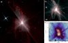 |
Fig. 1. False-colour images of NGC 6240 produced combining the MIRI images (see Sect. 2 for the details). Image a was obtained with the filters F560W and F1130W within an approximate FoV of 90″ × 90″ (1″ = 526 pc). Image b was obtained with the filters F770W and F1130W within an approximate FoV of 80″ × 80″ and the nuclei saturated to highlight the low-level structure. Panel c shows a zoom-in (approximate FoV of 7″ × 8″) to the F560W-filter image in logarithm scale with the position of the two radio sources in Gallimore & Beswick (2004) marked as blue crosses. The twelve contour levels in panel c go from 0.2% up to 73% of the flux peak, also in logarithm scale. We note that the diffraction spikes produced by the unresolved component of both nuclei have not been corrected. In all panels, north is up and east to the left. |
2.2. Emission line modelling
Once the data cubes were fully reduced, we modelled the emission line profiles to obtain their kinematics and flux maps. The fitting process involved several steps. First, we created an integrated spectrum for each nucleus with a circular aperture of 0.7″ (see Fig. 2). To fit the emission lines, we used the LMFIT library within PYTHON, allowing several different Gaussian components for each line, following Hermosa Muñoz et al. (2024a). We used the results from the integrated spectra as initial conditions for fitting each individual line on a spaxel-by-spaxel basis. Before the Gaussian fitting, we modelled and subtracted the local continuum. For that we selected a wavelength window on either side of the line that varied depending on the line’s width, while carefully avoiding other spectral absorption or emission features. Depending on the steepness of the continuum, we applied either a linear fit or a second-order polynomial function. To avoid spurious detections, we fitted the emission lines only when their signal-to-noise ratio (S/N) was higher than 3. We show some examples of the fitting in Fig. A.1.
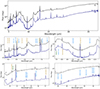 |
Fig. 2. Total integrated spectra for the northern (dark blue) and southern (black) nuclei of NGC 6240 obtained with a circular aperture of radius 0.7″. The top panel shows the full MRS spectral range after scaling the flux of some individual bands to match between them. The middle and bottom panels show the spectra per channel, with the main ionised gas emission lines indicated in blue, the H2 rotational lines in yellow, and the recombination H I lines in green. The wavelength is in rest frame assuming a redshift of 0.02448 (see Sect. 2). We applied a residual fringe correction for the 1D extracted spectra in ch3 and ch4 (see Argyriou et al. 2023). |
Some lines, such as [S IV] at 10.51 μm or [Ar III] at 8.99 μm, are embedded within the broad 9.7 μm absorption feature that complicates a correct determination of the continuum and the line flux. For those, we spatially re-binned the corresponding data cube with a box of 2 × 2 pixels to improve the S/N and obtain a better modelling of the line. These lines are properly indicated throughout the paper.
For correcting the velocities for the systemic value, we assumed a redshift of z = 0.02448 (Downes et al. 1993), which coincides with the systemic velocity derived from ALMA data (see e.g. Cicone et al. 2018; Treister et al. 2020). Using the velocities derived for the primary component of the warm molecular gas detected with MRS/MIRI for both nuclei (see Hermosa Muñoz et al., in prep.) we found a similar value for the redshift. After modelling the Gaussian profiles, we obtained the velocity dispersion and corrected it for instrumental broadening (see Argyriou et al. 2023) using  .
.
To obtain the global properties of the integrated emission lines, we additionally used a non-parametric analysis, based on Harrison et al. (2014) (see also Speranza et al. 2024; Hermosa Muñoz et al. 2024b). This allowed us to measure the parameters v02, v10, v50, v90, and v98, corresponding to the velocities at which the flux is 2%, 10%, 50%, 90%, and 98% of the total integrated flux of the line. Similarly to the parametric modelling, we defined the line for spectral elements where the flux is larger than three times the standard deviation from the local continuum. Examples of this modelling for several emission lines for both nuclei at different excitation levels are shown in Figs. A.2 and A.3. Additionally, we estimated the W80 parameter (tabulated in Table 2), which is equivalent to 1.088 times the FWHM for a Gaussian-like profile1. We did not estimate this parameter for the lines that are blended, such as [Ne V] at 14.32 μm and [Cl II] at 14.37 μm (see Sect. 3.1).
In general, we find that the emission lines with similar ionisation potentials (IPs) show similar kinematic properties. Thus, we focus on a few of the emission lines throughout the paper, and we show the kinematic and flux maps for the rest of the lines in Appendix B.
2.3. Modelling and subtraction of PAH features
In NGC 6240, the PAH features have a large contribution to the total flux of the spectra, potentially preventing the detection of some of the high excitation emission lines that fall within the same wavelength range (i.e. [Ne VI] and the PAH feature at 7.7 μm, see Fig. 2). However, for understanding the physical conditions and properties of the gas in this source, it is important to determine if these lines are indeed absent in the spectra, or if they are “buried” due to the strong PAH features.
In order to answer this question, we use the tool developed by Donnan et al. (2024) that models the near- and mid-IR continuum with different temperatures as well as the line and PAH emission taking into account differential extinction. For the purpose of the following analysis, it is sufficient to only model the mid-IR MRS spectra, as we are only interested in removing the bright PAH emission. The tool allows one to model the different PAH features (and emission lines) present in the mid-IR spectra and returns the properties of each individual component (e.g. central wavelength, equivalent width, flux, etc.). We applied this method only to the integrated spectra of the nuclei (R ∼ 0.7″), where the high excitation lines are expected to be brighter. We combined the individual PAH features to create a total PAH profile and subtract it from the integrated spectra. This allowed us to detect the high excitation lines that were initially buried for the S nucleus. The results from this modelling are presented in Sect. 3.5.
3. Results
With the MIRI/MRS data we have resolved for the first time the two nuclei in the 5−28 μm spectral range (see continuum maps in Fig. B.1). We present the integrated properties for both nuclei in Sect. 3.1, the main morphological properties and features of the ionised emission lines in Sect. 3.2, and the mid-IR line ratios in Sect. 3.3. We show the kinematical properties of the gas in Sect. 3.4, and the detection of the high excitation lines in Sect. 3.5. The non-parametric modelling for the integrated profiles for both nuclei is described in Appendix A.
3.1. Integrated properties of the nuclei
As already noticeable in Fig. 2, the two nuclei show different features in their spectra. The S nucleus is more luminous than the N nucleus (see Sect. 1), with stronger emission lines and PAH features, as already seen in Alonso-Herrero et al. (2014). We used the continuum maps of each band (see Fig. B.1) to determine the position of the nuclei. They are separated by an average distance of 1.6″ (1.7″ in channel 4 that has the lowest spatial resolution, see Sect. 1), and the same separation is measured using the F560W MIRI image (see Fig. 1). These positions are approximately coincident with the radio sources N1 and S, where the two AGN are believed to be located. The two radio sources are separated 1.5″ as reported by Gallimore & Beswick (2004), and coincident with the X-ray detected sources (Max et al. 2007). A more detailed discussion on the position of the nuclei based on NIRSpec observations is presented in Ceci et al. (2024).
We have detected a total of 20 different fine-structure emission lines with IPs ranging from 7.6 to 126 eV (see Table 1), two hydrogen recombination lines, namely Pfα and Huα (i.e. H I (6−5) at 7.46 μm and H I (7−6) at 12.37 μm, respectively), and 10 warm molecular (H2) emission lines (Hermosa Muñoz et al., in prep.). All these lines are indicated in Fig. 2. In general, the lines for both nuclei have very complex, non-symmetrical profiles, especially for the S nucleus. We have measured widths of at least 1000 km s−1 (FWHM), and even higher for some lines such as [Ne II] at 12.81 μm and [Ne III] at 15.55 μm in the S nucleus (see Fig. 3). As a result, lines close in wavelength, such as [Ne V] at 14.32 μm and [Cl II] at 14.37 μm, and [O IV] at 25.89 μm and [Fe II] at 25.99 μm, are blended in the spectra (see Fig. 3).
Flux measurements of the emission lines of NGC 6240 in the integrated spectra (r ∼ 0.7″) of both nuclei, ordered by ionisation potential.
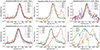 |
Fig. 3. Integrated profiles (r = 0.7″) of all the emission lines detected in the northern (upper panels) and southern (bottom panels) nucleus, after applying the fringing correction (see Sect. 2.1), normalised to the maximum flux. The lines are separated by IP, left IP < 25 eV, middle 25 < IP < 90 eV, and right IP > 90 eV. The rest-frame velocity corresponding to a z = 0.02448 is indicated with a dashed, grey, vertical line. We note that [O IV] is blended with [Fe II] at 25.99 μm and [Ne V] with [Cl II] at 14.37 μm (middle and right panels, see Sect. 3.1). We note that in the lower-right panel, [Ne VI] and [Mg V] are embedded in PAH features, and thus they are not detected in the original integrated spectrum (see Sects. 3 and 4.2). |
Despite the S nucleus being around three times brighter than the N nucleus, the latter shows strong high excitation emission lines (IP > 90 eV; e.g. [Ne VI] at 7.65 μm) that are barely detected for the S nucleus (see Fig. 2 and Sect. 3.5). These emission lines (e.g. [Ne V], [Ne VI], and [Mg V] at 5.6 μm2) can only be explained by AGN photoionisation (see e.g. Genzel et al. 1998; Sturm et al. 2002; Pereira-Santaella et al. 2022), whereas for lines such as [S IV] or [O IV] with intermediate IPs, and especially for lower ionisation potentials (see Table 1), star formation processes contribute the most to the emission (see e.g. Pereira-Santaella et al. 2010; Alonso-Herrero et al. 2012).
We present in Table 1 the measurements for the fluxes in the integrated spectra (r = 0.7″) for both nuclei. These fluxes are measured by modelling the profiles of the lines with a single Gaussian component. This is a simplification, given that for some lines the profiles are complex and a single Gaussian is not enough to fully reproduce their shape. However, we compared the line ratios obtained with these flux measurements and a simple integration of the line profile, and the values were similar (differences < 5%). We note that for the blended pairs [Ne V]+[Cl II], and [O IV]+[Fe II] at 25.99 μm we cannot integrate the profiles, so their fluxes were obtained with a two Gaussian modelling of the lines. From the flux measurements, the strongest ionised gas lines for both nuclei are [Ne II], [Ne III], [Ar II] at 6.98 μm, and [Fe II] at 5.34 μm.
The most relevant low excitation lines for this work (namely [Ne II], [Ne III], [Fe II] at 5.34 μm, and Pfα) are shown in Fig. 4, and the maps for the remaining lines are in Appendix B. We show in Fig. 5 the kinematic and flux maps obtained with a single Gaussian for the detected high-ionisation emission lines (namely [O IV], [Ne V], [Ne VI], and [Mg V]).
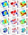 |
Fig. 4. Kinematic maps obtained with the modelling of a single Gaussian for the [Ne II], [Ne III], and [Fe II] at 5.34 μm and Pfα lines (from top to bottom, respectively). The latter line kinematics were obtained after re-binning the cube with a 2 × 2 box (see Sect. 2.2). From left to right: flux in erg s−1 cm−2, velocity in km s−1, and velocity dispersion in km s−1. The contours in the velocity maps go from −300 to 300 km s−1 (increments of 100 km s−1). The contours in the flux maps go from 10−16 to 10−14 erg s−1 cm−2 (divided in 5 contours), except for Pfα (from 10−17 to 10−15 erg s−1 cm−2). White stars indicate the photometric centre for both nuclei in their corresponding sub-channels, and the lower-left line indicate the 1″ physical scale. The (0, 0) point in each panel marks the centre of the FoV at each channel. For all maps, north is up and east to the left. |
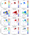 |
Fig. 5. Kinematic maps obtained with the modelling of a single Gaussian for the [O IV], [Ne V], [Ne VI], and [Mg V] lines, top to bottom. A full description is in Fig. 4. |
3.2. Morphological properties
In the MIRI images (see Fig. 1) we detect ionised gas emission extending ∼50 kpc in the north-south direction. In the inner parts of the image we detect the “Butterfly Nebula” (see Sect. 1), extending ∼5 kpc east-west, with a bubble-like structure towards the north-west part and several ionised gas filaments to the east and south (see also Medling et al. 2021).
Focusing on the inner regions studied with the MRS data, in the left panels of Figs. 4 and 5 we see that both low and high excitation lines show distinct morphological features. The ionised gas traced by the low excitation lines is detected across the entire FoV (see Fig. 4), with most of the emission concentrated around the two nuclei. The main features detected in the flux maps are indicated in Fig. 6 and described below. For all lines, the flux peaks at the S nucleus, although [Ne II] shows a bridge connecting both nuclei (see also Alonso-Herrero et al. 2014), which is not as prominent for [Ne III] (see also the [Fe II] map in Fig. B.2 and the PAH map in Fig. 7). There is, however, significant extended emission detected both to the north-west of the N nucleus and to the south-east (Ext1 in Fig. 6) and south of the S nucleus, seen most clearly in the [Ne II] and [Ne III] flux maps (namely Ext2 in Fig. 6, see also left panels in Fig. 4). Both regions roughly coincide with the molecular outflow and one of the ionisation cones detected with the NIRSpec data in (Ceci et al. 2024, see their Fig. 10). This Ext1 region coincides with the NES extension defined in Fig. 5 in Paggi et al. (2022) using soft X-rays. A few additional clumps are apparent in the flux maps, labelled C1 (at ∼2″ or projected distance ∼1 kpc west from the S nucleus), C2 (at ∼3.8″ or projected distance ∼2 kpc east of the N nucleus), and C3 (at ∼3″ or projected distance ∼1.6 kpc southeast of the S nucleus). The C3 clump is seen directly in the MIRI images (see Fig. 1), but for the MRS it is only detected in ch3 and ch4 due to their larger FoVs (see Sect. 2). The region around C2 coincides with the “Outflow ridge” defined with soft X-ray data (see Fig. 5 in Paggi et al. 2022). In general, there is little correspondence between the morphological features in the flux maps and those in the kinematic maps (see Sect. 3.4), although C1 coincides with a high velocity dispersion region (σ ∼ 500 km s−1) for both neon lines. In general, we find that the morphology of the ionised gas (see Figs. 4 and B.2) closely resembles that of the 0.3 − 3 keV X-ray emission (see Fig. 2 in Paggi et al. 2022), as already noted in several other studies (Nardini et al. 2013; Yoshida et al. 2016; Paggi et al. 2022).
In Fig. 7 we show the flux map of the PAH feature at 6.2 μm, obtained by integrating over its total wavelength range (6.15 μm to 6.5 μm) after subtracting a linearly interpolated continuum estimated from points at either side of the feature. As for the low excitation lines, the peak of the flux is located in the S nucleus, and we clearly detect the bridge between both nuclei. The extended emission towards the south-east from the S nucleus (Ext1 in Fig. 6) is also detected.
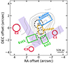 |
Fig. 6. Schematic figure of the main features seen in the flux and kinematic maps of the emission lines superimposed onto the [Ne III] flux map contours (see Fig. 4). In red we mark the position of the different detected clumps (namely C1, C2, and C3), and in green are the extended emission regions (namely Ext1 and Ext2, see Sect. 3.2). The bubble-like structure mainly detected with the high-excitation lines is in blue (extending up to ∼5.2″, i.e. 2.74 kpc; see Fig. 5 and Sect. 4.3), and the bridge detected between both nuclei (separated ∼1.6″, i.e. ∼840 pc; see Sect. 3.1) is marked in yellow. The purple regions indicate the V-shaped structure detected in the velocity dispersion maps. Additionally, we mark with black, dashed circles the region where we integrated the spectra for both nuclei, as well as their position with the white stars. |
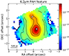 |
Fig. 7. Flux map of the PAH feature at 6.2 μm in log scale estimated after subtracting a local continuum from both sides of the feature. The contour levels go from 10−16 to 10−14 erg s−1 cm−2. |
The extended emission detected to the north-west of the N nucleus is even more evident in the high excitation line emission (see Fig. 5). These high excitation lines (IP > 50 eV) are only detected in and around the N nucleus in the pixel-by-pixel modelling. They expand mainly in a bubble-like shape towards the north-west region at a PA of ∼25° (measured west to north from the N nucleus), with similar morphologies for [Ne VI], [Mg V], and [Ne V]. The [O IV], which is observed in the larger FoV ch4-long channel (see Sect. 2.1), reveals some emission to the south-east at ∼4″ (projected distance ∼2.1 kpc) from the N nucleus (namely C2, see Fig. 6) at a similar PA that the NW emission. This emission is coincident with the beginning of the east arm detected with [O III] in Müller-Sánchez et al. (2018) (see also Medling et al. 2021).
3.3. Mid-IR line ratios
In general, the low excitation lines such as [Ne II] are typically ionised by star formation processes and/or shocks, whereas the high excitation lines (IP > 90 eV) such as [Ne V] can only be produced by AGN photoionisation. As mentioned in Sect. 3, the emission lines with intermediate IPs (IP > 25 eV) can be produced due to ionisation from both stars and AGN; thus they tend to show more complex kinematics and flux properties (see also Armus et al. 2023; Dasyra et al. 2024; Hermosa Muñoz et al. 2024b). We used the mid-IR line ratios obtained by Pereira-Santaella et al. (2010), in particular [Ne V]/[Ne II], [Ne III]/[Ne II], [O IV]/[Ne II], and [O IV]/[Ne V], to disentangle the main ionising source of the different regions in NGC 6240. First, we obtained the overall properties of the nuclei with the integrated line ratios (r ∼ 0.7″), using both high and low excitation lines. We found that for the N nucleus, all ratios using the Neon and [O IV] lines are consistent with those found in LINERs and/or star-forming regions (Pereira-Santaella et al. 2010): [O IV]/[Ne V] = 4.20 (0.62 in log); [O IV]/[Ne II] = 0.14 (−0.86 in log); [Ne III]/[Ne V] = 11.9 (1.08 in log); and [Ne V]/[Ne II] = 0.03 (−1.49 in log). As for the S nucleus, all the line ratios are consistent with star-forming regions (Pereira-Santaella et al. 2010): [O IV]/[Ne V] = 9.9 (1.0 in log); [O IV]/[Ne II] = 0.04 (−1.44 in log); [Ne III]/[Ne V] = 67.7 (1.8 in log); and [Ne V]/[Ne II] = 0.004 (−2.438 in log). However, using the [O IV] ratios, if we put both nuclei in Fig. 6 in Hernandez et al. (2023), the S nucleus lies between the starburst-dominated systems, whereas the N nucleus falls in the AGN-dominated region.
Additionally, we created a [Ne III]/[Ne II] line ratio map in Fig. 8 (top panel), as [Ne III] is the line with the highest IP (41 eV) detected in single-spaxel spectra across the entire FoV, including the S nucleus. In general, the ratio is low (median of −0.44 and standard deviation of 0.16 in logarithm scale), and consistent with those found in LINERs in Pereira-Santaella et al. (2010). The various regions identified in the flux maps (see Fig. 6) also show clear differences in their line ratios. The highest (lowest) ratios are located towards the northern (southern) part of the FoV. We find the minimum around the S nucleus (average value of −0.82 ± 0.08 in log) and towards the extended emission Ext1 (see Fig. 6). The region of the bubble, located west of the N nucleus, and C2, located ∼3.8″ east of it, have the highest ratios (> − 0.1 in log). Following again Pereira-Santaella et al. (2010), these ratios are closer to those expected for regions photoionised by a Seyfert nucleus. Also, the extended region west of the N nucleus, C2, is oriented similarly to the bubble-like structure clearly seen in the high excitation lines. We also created a [Fe II] at 5.34 μm over [Ar II] map, shown in the bottom panel of Fig. 8. This ratio could be useful for disentangle between shocks (using [Fe II]) and SF (traced by [Ar II]). The minimum values of this ratio (∼0.5) are located in both nuclei and in the bubble region. However, the maximum values (∼1.2) are located in the bridge between both nuclei, which could be tracing shocks produced by the interaction between the original galaxies and in the extended region Ext1. We further discuss these ratios and their comparison to optical diagnostics in Sect. 4.1.
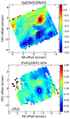 |
Fig. 8. Line ratios between [Ne III] and [Ne II] in log scale (upper panel) and [Fe II] over [Ar II] in linear scale (bottom panel). In the top panel we superimpose the contours from the [Ne III] flux map (see Fig. 4). The white stars indicate the position of both nuclei. |
3.4. Kinematical properties
We represent in Fig. 3 the profiles of the emission lines detected in the integrated spectra (see Fig. 2). When simply integrating, the high excitation lines in the S nucleus are not clearly detected ([Mg V] and [Ne VI] are inside a PAH feature, as shown in lower-right panel of Fig. 3). From the emission line profiles, it is clearly seen that the two nuclei have different rest-frame velocities. In the N nuclei, the maximum is shifted by ∼100 km s−1 after correcting for the redshift (see Sect. 1), but for the S nucleus the peak is shifted by −100 km s−1 for all the detected lines (see v50 parameter in Table 2). For some lines, such as [Ne II] or [Ne III], there is a prominent redshifted wing reaching velocities > 1000 km s−1 for the S nucleus, which was similarly detected for the molecular gas (see e.g. Cicone et al. 2018).
3.4.1. Non-parametric modelling
From the non-parametric analysis (see Sect. 2.2), we found that the average value for the W80 parameter is ∼600 km s−1 for the N nucleus, while the S nucleus presents systematically larger widths, up to ∼1400 km s−1. From Table 2, it is clear that the low excitation lines tend to have lower widths than the high excitation lines. Dasyra et al. (2011) suggested that, if the narrow line region of the AGN is stratified, then the lines with higher IPs would have larger FWHM that those with lower IPs. This would be due to the fact that they originate closer to the AGN and thus are more affected by the strong motions taking place in the inner regions. These trends have been seen for other objects (Armus et al. 2023), such as the type-2 Seyfert NGC 7172 (see Hermosa Muñoz et al. 2024b). We have plotted the W80 parameter versus the IP for the N nucleus, where we detect lines at all IPs, and we only detected a trend with moderate significance (ρ ∼ 0.07 and p-value ∼ 0.79). We did not detect a trend of the derived velocities with the IP of the lines. In terms of the largest velocities characterised with the v02 and v98 parameters, overall, the velocity structure of the lines spans more than 800 km s−1 and up to ∼1300 km s−1 (N) and ∼2000 km s−1 (S) for lines such as [Ne III]. Although the rotational motions contribute to the line widths, these high velocities and the highly asymmetric line profiles are typically attributed to the presence of non-rotational motions such as outflows (see discussion in Sect. 4.3).
3.4.2. Parametric modelling
As mentioned in Sect. 3.1, the line profiles are complex and this makes it challenging a proper decomposition and ordering of all the components within the FoV. We tried modelling the ionised gas emission lines on a spaxel-by-spaxel basis using a multi-Gaussian approach. At least two Gaussians are found across most of the FoV, but there are additional broad components and visible double peaks particularly towards the south-west and south-east regions. In addition, for the two nuclei, the different components blend together, generating very broad profiles that cannot be easily disentangled, especially at the longest wavelengths. All of this makes it difficult to correctly follow the individual kinematic components across the FoV, and associate them consistently with a particular physical process. Thus, we decided to just discuss the overall kinematic properties using a one Gaussian fitting, but we show some examples of the multi-Gaussian modelling of the integrated line profiles for both nuclei in Fig. A.1. We discuss and compare the non-parametric approximation and the parametric results in Appendix B.
We have estimated the kinematic and flux maps for all lines with a single Gaussian component, which are equivalent to moment 0 and moment 1 maps (see examples of the maps for the main lines in Figs. 4, 5 and B.2). As mentioned in Sect. 3.2, for all the high-ionisation emission lines we detect the peak of the emission at the N nucleus, and some extended emission up to 2″ towards the north-west. Additionally, we detect some extended [O IV] emission ∼4″ east of the nucleus. For all the lines the global kinematic properties (i.e. velocity and velocity dispersion, σ) are very similar. The nuclear region shows higher values of the velocity dispersion (σ∼300 km s−1) than the north-west, extended region (σ ∼ 150 km s−1). The lines are completely redshifted with velocities of up to 300 km s−1 except at the nucleus, where the lines are at almost rest-frame values. However, the low and intermediate ionised emission line kinematics show a more complex picture.
In Fig. 4 we present flux maps of the [Ne II] and [Ne III] lines, modelled with a single Gaussian. These are representative for other lines with similar IPs while covering a larger FoV (see also Fig. B.2). The velocity and velocity dispersion maps are highly disturbed, i.e. do not follow a classical rotation pattern. As mentioned in Sect. 3.2, this makes it difficult to associate their morphology with any particular kinematic feature(s). In general, the kinematic maps for both lines are similar, with the redshifted velocities (up to 500 km s−1) located towards the northern and eastern part of the FoV and the blueshifted (down to −600 km s−1) mainly towards the west from the S nucleus. The region around the N nucleus has almost rest-frame velocities and a velocity dispersion of ∼300 km s−1 for both [Ne II] and [Ne III] lines. However, the region around the S nucleus is blueshifted for both lines (v ∼ −100 km s−1) with larger velocity dispersion (σ ∼ 400 km s−1). This velocity difference was already hinted at in the analysis of the integrated spectra of the nuclear regions (see Table 2).
The velocity dispersion is highly disturbed, with the highest values (σ > 400 km s−1) distributed in a V-like shape extending from the north-east part towards the south-west part, passing through the S nucleus. It is particularly enhanced towards the south-west region (maximum σ ∼ 590 km s−1 for [Ne III], see bottom left panel in Fig. 4), where the more blueshifted velocities are found. In contrast, the bubble region has redshifted velocities (up to ∼200 km s−1) and low velocity dispersion (∼250 km s−1 for [Ne II] and ∼200 km s−1 for [Ne III]), consistently to the kinematic properties derived from the high excitation line (see Fig. 5).
There is a region at the limits of the FoV to the southeast from the S nucleus (C3 in Fig. 6) with almost rest-frame velocities and very low velocity dispersion (∼50 km s−1) that is clearly seen as a blob in [S III] (see Fig. B.2). This region is also detected in the [Ar II] map and in the F560W filter MIRI image, located at 3″ SE (61° east to south) from the S nucleus. It is likely a SF region corresponding to one of the clusters previously detected in this system (see Pollack et al. 2007).
3.5. High ionisation emission lines
As mentioned in Sect. 3.2, evaluation of the high excitation lines on a spaxel-by-spaxel basis is only possible around the N nucleus, likely because the S nucleus emits a much brighter MIR continuum (see e.g. Puccetti et al. 2016). The largest difference for the continuum emission between nuclei is found at the longest wavelengths (factor ∼ 4; see Fig. 2 and also Fig. B.1). This could impact the detection of high ionisation emission lines both in the spatially resolved (see Fig. 5) and the integrated analysis of the S nucleus (see Fig. 3).
From the spectra in Fig. 2, it is clear that in both nuclei of the NGC 6240 system, the emission from PAH features is intense and complex, thus hampering the detection and characterisation of weak emission lines. This is particularly true for [Ne VI] and [Mg V] lines, which lie inside a PAH feature at 7.7 μm and 6.2 μm, respectively. In fact, there is PAH emission all over the mapped FoV (see the 6.2 μm PAH feature map in Fig. 7, and see also Alonso-Herrero et al. 2014 for the PAH feature at 11.3 μm), which is particularly prominent around the S nucleus and slightly fainter in the N nucleus and in the bridge connecting the two nuclei, similarly to [Fe II] (see Sect. 3.4 and Fig. B.2).
For these reasons, to properly detect and characterise the high excitation lines in both nuclei, we model and subtract the PAH emission from the integrated spectra using the tool developed by Donnan et al. (2024) (see Sect. 2.3).
We show in Fig. 9 the results for the PAH-subtracted spectra of both nuclei, highlighting the region around the [Mg V], [Ne VI], Pfα, and [Ne V] emission lines. As already mentioned, the first three overlap with a PAH feature, whereas the [Ne V] is in a wavelength range less affected by the PAH features (Chown et al. 2024). The main result is that when subtracting the PAH model from the observed spectrum, the high excitation lines [Mg V] and [Ne VI], as well as Pfα, are now detected in the S nucleus. For the particular case of [Ne VI], the line is still contaminated by the presence of the absorption due to the ice CH4 band at ∼7.7 μm. This demonstrates that in the S nucleus, these lines are indeed buried by the strong continuum and dust features, similarly to what has been proposed for Arp 220 (Perna et al. 2024), II Zw96 (García-Bernete et al. 2024), or for Mrk 231, where the weak X-ray nature of its AGN likely also contributes to the absence of high-excitation lines (Alonso Herrero et al. 2024). In Table 1 we report the flux measurements for [Mg V] and [Ne VI] after the PAH subtraction for both nuclei. These lines are broader in the S nucleus than in the N nucleus (![Mathematical equation: $ \sigma_{\mathrm{[Ne\,VI]}}^{\mathrm{S}} = 357\pm36 $](/articles/aa/full_html/2025/01/aa52437-24/aa52437-24-eq2.gif) km s−1 vs
km s−1 vs ![Mathematical equation: $ \sigma_{\mathrm{[Ne\,VI]}}^{\mathrm{N}} = 222\pm5 $](/articles/aa/full_html/2025/01/aa52437-24/aa52437-24-eq3.gif) km s−1, and
km s−1, and ![Mathematical equation: $ \sigma_{\mathrm{[Mg\,V]}}^{\mathrm{S}} = 526\pm17 $](/articles/aa/full_html/2025/01/aa52437-24/aa52437-24-eq4.gif) km s−1 vs
km s−1 vs ![Mathematical equation: $ \sigma_{\mathrm{[Mg\,V]}}^{\mathrm{N}} = 279\pm9 $](/articles/aa/full_html/2025/01/aa52437-24/aa52437-24-eq5.gif) km s−1), similarly to what we found for the rest of the emission lines (see Table 2).
km s−1), similarly to what we found for the rest of the emission lines (see Table 2).
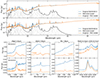 |
Fig. 9. Full integrated (r ∼ 0.7″) spectrum of the two nuclei in rest frame after modelling the dust features and continuum (see details in Sect. 4.2). The upper figures show the global fit to the S (top) and N (bottom) nucleus before (blue) and after (orange) subtracting the total PAH emission (black). The modelled contribution of the individual PAH features are shown in grey. The bottom panels show some insets near the region of [Mg V], Pfα, [Ne VI], and [Ne V] lines for both nuclei. The rest-frame wavelengths are indicated with a dashed, grey, vertical line. The Pfα and [Ne VI] lines from the S nucleus have been scaled for visualisation purposes. |
Even after PAH modelling and subtraction, the [Ne V] line for the S nucleus is still not detected with good S/N in the data ([Ne V] at 24.32 μm is not detected), although it is clearly detected in the N nucleus. This line is blended with [Cl II] and both are broad, like other lines with similar IPs. This would dilute the line and hamper a good detection given the strong continuum in the S nucleus. Moreover, [Cl II] is stronger in the S nucleus than in the N nucleus with respect to [Ne V], which suggests that the relative contribution of the star formation is larger in the S nucleus. The strong contribution from the continuum is likely the cause for the non-detection for other lines, such as the [Ar V] at 7.9 μm and at 13.1 μm (IP of 59.6 eV), which is detected in the region of the bubble structure seen in the spatially resolved maps (see Figs. 5 and 6) but not in the nuclear apertures (see Fig. 2). We discuss the detection of the high excitation lines in Sect. 4.2.
4. Discussion
NGC 6240 is an interacting system in a merging phase (van der Werf et al. 1993; Engel et al. 2010; Fyhrie et al. 2021). From the results presented in Sect. 3 and from previous works (see Sect. 1), there are several processes occurring simultaneously in this galaxy, affecting the gas kinematics and distribution. The stellar discs of the two galaxies were clearly detected using near-IR observations (Medling et al. 2014; Ceci et al. 2024). However, based on our results as well as in optical observations (Müller-Sánchez et al. 2018), the ionised gas is decoupled from the stellar emission. The velocity maps do not show a regular rotating pattern anywhere along the FoV, although there is a clear shift between the velocities from both nuclei (see Sect. 3.4), previously detected also with the stellar component (Kollatschny et al. 2020). The existence of multiple intensity peaks and kinematic components in the emission lines points towards a highly perturbed and shocked gas as a result of the interaction between the initial galaxies and the triggering of both the AGN and the starburst activity. All these perturbations are likely producing the apparent lack of correlation detected between the morphologies and kinematic properties of the emission lines (see Figs. 4, 5, and B.2).
In Sect. 4.1 we discuss the origin of the ionised gas based on our mid-IR line ratios. We explore in Sect. 4.2 about the presence and detection of the high excitation lines for this source and other AGN observed with the JWST. Finally, we give evidence about the presence of outflows in the system and their properties as seen in the mid-IR in Sect. 4.3.
4.1. Origin of the ionised gas
From optical line ratios, the N nucleus was previously associated with LINER-like photoionisation, and the S nucleus with Seyfert-like photoionisation (e.g. Müller-Sánchez et al. 2018). However, other works in the literature have detected the presence of multiple shocked regions throughout the system (see e.g. Fosbury & Wall 1979; van der Werf et al. 1993; Nardini et al. 2013; Medling et al. 2021). This would explain the LINER-like ratios around the N nucleus, given the degeneration in optical diagnostic diagrams between shock models and LINERs (Heckman 1980; Baldwin et al. 1981; Dopita & Sutherland 1995). In general, the [Ne III]/[Ne II] ratios (see Fig. 8) are consistent with observational measurements derived with Spitzer for galaxies classified as H II/LINER (Pereira-Santaella et al. 2010). They are also consistent with the presence of shocks except for the region north-west of the N nucleus (bubble in Fig. 6), which has ratios similar to those observed in Seyfert galaxies (see Pereira-Santaella et al. 2010). Moreover, the detection of high excitation lines in the N nucleus, such as [Mg V], [Ne VI], and [Fe VIII] provides evidence that it is indeed an AGN.
4.1.1. Nuclear regions
The majority of the central region of NGC 6240 is consistent with being dominated by shocks and by SF ionisation, as previously suggested. In Fig. 10 we show a simplified version of the diagnostic diagrams from Fig. 5 in Feltre et al. (2023), comparing the ratios of different neon transitions. We found that the N nucleus has log([Ne III]/[Ne II]) = −0.42 ± 0.01 and log([Ne V]/[Ne II]) = −1.49 ± 0.02 (measured with r ∼ 0.7″, see Table 1), which are consistent with AGN+shock ionisation according to the diagram. For the S nucleus, on the other hand, we measured a ratio log([Ne III]/[Ne II]) = −0.61 ± 0.04 and log([Ne V]/[Ne II]) = −2.44 ± 0.08. If we compare with other models in Feltre et al. (2023) (see also Allen et al. 2008; Sutherland & Dopita 2017; Alarie & Morisset 2019), the shocked regions reach the lower-left part of the diagram, indicating that the ratios for both nuclei are consistent with shocks. With Spitzer/IRS data, Armus et al. (2006) also derived the line ratios encompassing both nuclei, finding similar values to our determination for the N nucleus (log([Ne III]/[Ne II]) ∼ −0.45 and log([Ne V]/[Ne II]) ∼ −1.52, uncorrected for extinction, see Fig. 10). This is expected, as the contribution from the [Ne V] emitted in the N nucleus is larger than for the S nucleus (see Table 1 and Fig. 2). They stated that these ratios are consistent with being excited by the presence of a nuclear starburst.
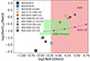 |
Fig. 10. Mid-IR diagnostic diagram representing log([Ne V]/[Ne II]) versus log([Ne III]/[Ne II]) to divide between AGN (red area), shocks (green area), and SF (purple line) ionisation based on Fig. 5 in Feltre et al. (2023). The shaded areas schematically represent part of the grid of models in Feltre et al. (2023), and are used here just as a reference. We represent with a blue and a black star the position of the N and S nucleus, respectively (see Sect. 3.3). For comparison, we show the integrated value derived by Armus et al. (2006) for NGC 6240 as a white circle, and the nuclear values obtained with similar JWST data for other local type-2 Seyfert galaxies: yellow circle for NGC 7172 (Hermosa Muñoz et al. 2024b), orange circle for NGC 6552 (Álvarez-Márquez et al. 2023), dark (light) green triangles for the total (primary component) flux of the line for the type-1.5 Seyfert NGC 7469 (Armus et al. 2023), and red circle for NGC 7319 (Pereira-Santaella et al. 2022). Additionally, we show the ratios for two LINERs, namely NGC 4594 and NGC 1052, as a blue and brown squares, respectively (Goold et al. 2024). |
Additionally, for comparison we show in Fig. 10 the nuclear regions of other local Seyfert galaxies (namely, type-2s NGC 7319, NGC 6552, and NGC 7172, and the type-1.5 NGC 7469) and LINERs (namely, NGC 1052 and NGC 4594) observed with JWST MIRI/MRS data (Pereira-Santaella et al. 2022; Álvarez-Márquez et al. 2023; Armus et al. 2023; Hermosa Muñoz et al. 2024b; Goold et al. 2024). These Seyfert galaxies present ratios consistent with AGN photoionisation that are very different from those derived with NGC 6240. Contrarily, both nuclei lie in a similar region of the diagram to the two LINERs (particularly the N nucleus), indicating that SF and shocks have a dominant role in the ionisation of the nuclear region emission. This is despite the detection of high excitation lines associated with AGN photoionisation. This implies that, as previously proposed (Tecza et al. 2000; Armus et al. 2006; Engel et al. 2010), the AGN are not the main source of ionisation for the ISM in the mid-IR.
If instead we estimate log([Ne III]/[Ne II]) for the two nuclei of NGC 6240 by separating the line profiles into different Gaussian components (see Appendix A and Fig. A.1), we get a similar ratio for both nuclei and both the narrowest, primary component and the broadest, secondary component (N nucleus −0.48 ± 0.03 vs −0.39 ± 0.02 in log, respectively; S nucleus −0.66 ± 0.02 and −0.57 ± 0.02 in log, respectively). Nevertheless, in both cases the ratios fall in the same region in the mid-IR diagrams by Feltre et al. (2023) as for the ratios obtained with the integrated fluxes (see Fig. 10).
4.1.2. SF emission
Various works from the literature detected significant enhanced emission in between both nuclei (the bridge region, see Fig. 6), associating it to a nuclear starburst (see e.g. van der Werf et al. 1993; Lutz et al. 2003; Müller-Sánchez et al. 2018), while ground-based spectroscopy detected the brightest 11.3 μm PAH emission around the S nucleus (Alonso-Herrero et al. 2014). From the maps derived for the PAH feature at 6.2 μm (see Fig. 7 and Sect. 3.2), we detect the maximum of the emission at the S nucleus, ∼6 times more intense than in the N nucleus and ∼9 times more than the bridge region. As mentioned in Sect. 3.2, the same applies for emission lines such as [Ne II] and other low excitation lines (see Figs. 4 and B.2), which are mostly ionised by SF processes. In fact, from the [Fe II]/[Ar II] map (bottom panel in Fig. 8) the nuclei show the lowest ratios, indicating that SF is stronger there. Finally, from the [Ne III]/[Ne II] spatially resolved line ratios in Fig. 8, we detected the lowest ratios for the region around the S nucleus, which may also indicate that the relative contribution from the SF processes is larger than in other regions, such as the bridge between both nuclei. To quantify this, we used the relations from Eq. (12) by Shipley et al. (2016), which relates the star formation rate (SFR) to the luminosity of the different PAH features. Using the fluxes measured in the integrated spectra with the tool by Donnan et al. (2024) (see Sect. 3.5), we found that the SFR of the S nucleus is ∼4.1 times larger than that of the N nucleus. Thus, although there is possibly SF occurring in the bridge and in the N nucleus, the peak of the nuclear starburst is detected in the S nucleus.
4.1.3. Shocked emission
Another way to evaluate the presence of shocks is by means of the [Fe II] lines, which are a tracer of both shocks and star-forming processes (see e.g. Allen et al. 2008). In Fig. 4 we show the kinematic maps for the [Fe II] at 5.34 μm, as it is the iron line detected with the best S/N (see spectra in Fig. 2). We note, however, that it covers the smallest FoV as it is located in ch1-short (see Sect. 2). There is [Fe II] emission arising in the nuclei as well as the bridge region, with similar velocities and velocity dispersion to other low excitation lines, with σ particularly enhanced west from the S nucleus. Given the complex profiles detected in that region for both ionised and the warm molecular gas (Hermosa Muñoz et al., in prep.), it is likely that shocks are simultaneously affecting all the gas phases. This is consistent with the picture drawn from the near-infrared line ratios, particularly that of H2 1−0 S(1) over Paβ (Medling et al. 2021). This ratio is high when the molecular gas is excited by shocks, and in fact it shows large values all over the system probably due to the interaction of the galaxies (see also van der Werf et al. 1993). It is especially enhanced in the region in between nuclei, west of the S nucleus, and along the direction of the detected [O III] outflow (see Müller-Sánchez et al. 2018). This enhanced, bridge region (see Fig. 6) was proposed to be shocked gas as a consequence of the interaction between the galaxies (see e.g. Tecza et al. 2000; Max et al. 2005). From the [Fe II]/[Ar II] ratio (bottom panel in Fig. 8), the largest values are also in the bridge region, which supports this hypothesis.
Based on the optical line ratios reported by Medling et al. (2021), despite the significant dust obscuration (with Hα/Hβ ∼ 20, larger in the region between the two nuclei), both nuclear regions fall within the AGN regime. Most of the other regions are consistent with either AGN+shocks or LINER+shocks, which aligns with the mid-IR ratios observed in this work. Moreover, as mentioned in Sect. 3.2, there is a spatial coincidence between the features traced with the soft X-rays and the ionised gas (see also Nardini et al. 2013; Yoshida et al. 2016; Paggi et al. 2022). The C2 region partly coincides with the largest ‘outflow ridge’ region defined in Fig. 5 in Paggi et al. (2022), which was consistent with shock excitation. The bubble region, which forms part of the largest Hα bubble detected in the optical (Müller-Sánchez et al. 2018) and the X-ray loop (Paggi et al. 2022) is however associated with a starburst-driven outflow.
4.2. Detection of high excitation lines in deeply embedded nuclei with mid-IR data
As mentioned in Sect. 1, the S nucleus has approximately three times larger bolometric luminosity than the N nucleus (Müller-Sánchez et al. 2018), and is brighter by a factor ∼2.6 in both soft and hard X-rays (i.e 10−40 keV luminosity of 7.1 × 1043 erg s−1 and 2.7 × 1043 erg s−1, for the S and N nucleus respectively, Puccetti et al. 2016). The high X-ray luminosities classify both nuclei as AGN (Puccetti et al. 2016; Paggi et al. 2022). As seen in Sect. 3.5, the mid-IR continuum emission is brighter for the S nucleus, and it is impacting on the detection of high excitation lines in our data. However, although we have detected [Ne VI] and [Mg V] for both nuclei, the [Ne V] line is still seen with low S/N for the S nucleus.
One possibility proposed to explain the lack of high excitation lines in some U/LIRGs is the presence of high extinction. Yamada et al. (2024) proposed that U/LIRGs with high column densities (NH from 1022 to 1024 cm−1) may not show [O IV] and [Ne V] emission. For the particular case of NGC 6240, Komossa et al. (2003) derived a column density of 1−2 × 1024 cm−2 with Chandra data for both nuclei, which suggest that they are highly absorbed, although there are other determinations (∼1022 cm−2 in Paggi et al. 2022). From the H2 molecular lines we derived the column densities for both nuclei and found values below 1022 cm−2 (Hermosa Muñoz et al., in prep.). Although indeed the S nucleus shows larger extinction than the N nucleus, we do not detect a significant difference between both. We estimated τ9.8 ∼ 2 vs 1.8, respectively, for the H2 emission using the tool by Donnan et al. (2024, see Sect. 3.5).
Another plausible explanation is that the stronger dust emission, in the form of continuum and PAH features, in the S nucleus hinders the detection of the lines. From our results presented in Sect. 3.5, this seems to be likely the case for NGC 6240. The PAH features hamper the measurements of the emission lines for both nuclei. Even in spectral regions with no PAH emission (e.g. close to the [Ne V] lines), the continuum is strong. From the [Ne V] and [Cl II] complex (see lower right panels in Fig. 9), the relative contribution of [Cl II] with respect to the [Ne V] changes between nuclei (see Sect. 3.5). Particularly, for the S nucleus the brightest [Cl II] indicates that SF is stronger than for the N nucleus, consistently with the derived SFRs in Sect. 4.1.2. Additionally, the lines for the S nucleus are broader than for the N nucleus, which contributes to dilute the [Ne V] line if the [Cl II] is also broad and brighter. Thus for the S nucleus, the low contrast of the high excitation emission lines is likely a combination of a strong mid-IR continuum, very broad lines, and intense SF in the nucleus.
In other local U/LIRGs even with JWST observations, high excitation lines remain undetected, for instance, in Mrk 231 (Alonso Herrero et al. 2024), Arp 220 with NIRSpec (Perna et al. 2024) and MRS (Goldberg et al. 2024; Rieke et al., in prep.; van der Werf et al., in prep.), and II Zw96 (García-Bernete et al. 2024). For Mrk 231, the non-detection of high excitation lines is likely due to both the intrinsically faint X-ray nature of the source and the strong mid-IR continuum (Alonso Herrero et al. 2024), while for Arp 220 the main reason is probably the high levels of obscuration (Goldberg et al. 2024) or that this source is not an AGN (van der Werf et al., in prep.; Buiten et al., in prep.). Thus the detection of high excitation lines in deeply embedded AGN depends on their exact nature and intrinsic properties.
4.3. AGN-driven outflow detection and properties
The emission detected with a bubble-like shape towards the north-west part of the galaxy is most likely an expanding outflow. In fact, it is identified as an ionisation cone with the NIRSpec data (Ceci et al. 2024). It is coincident with the base of the Hα bubble to the west and the [O III] cone to the east detected on much larger scales (Müller-Sánchez et al. 2018). The Hα bubble was associated with the most recent starburst episode in the system, given its kinetic energy and the derived time scale of the event (Müller-Sánchez et al. 2018). However, the kinetic power derived for the [O III] outflow was insufficient to be solely attributed to the starburst, so Müller-Sánchez et al. (2018) concluded that it has to be AGN-driven. They estimated a mass outflow rate, Ṁout, of 75 M⊙ yr−1 for the [O III] cone, and of 10 M⊙ yr−1 for the Hα bubble, though they state that these are probably lower limits to the total mass.
We detect an expanding bubble clearly traced by high excitation lines such as [Ne V], [Ne VI], and [Mg V] (see Fig. 5), as well as intermediate excitation lines, such as [Ar III] and [S IV] (see Fig. B.2), and also Pfα. This feature, extending up to ∼5.2″ (i.e. projected distance of 2.74 kpc) from the N nucleus (see Fig. 5), appears to be a gas flow expanding at receding velocities, likely associated with the large-scale Hα bubble. However, the complicated kinematics, with broad line widths and wings detected in both nuclei (see Sect. 3.4), suggest the presence of additional non-rotational motions. In particular, the S nucleus exhibits a line component of σ ≥ 600 km s−1 (see Fig. A.1), which could only be explained by the existence of strong gas motions, likely driven by complex interactions within the system, and associated with the large scale outflows. Due to the contamination from the SF emission, we cannot spatially resolve the outflow located in and/or around the S nucleus using the intermediate or low excitation emission lines. Thus, here we focus on the integrated properties of the southern nuclear outflow, while the N nucleus is already included within the bubble region.
To estimate the properties of the ionised gas outflows, Hα (or Hβ) and [O III] are typically used. Although the NW bubble is better traced by the high excitation lines, and thus we could use the [Ne V] line to estimate the outflow properties (see e.g. Zhang et al. 2024). We used the Pfα line, which is detected in both nuclei, for consistency in the measurements. This hydrogen recombination line is detected in the NW bubble and in both nuclei with sufficient S/N (> 3, see Sect. 2.2). Moreover, it traces a similar emission to other hydrogen transitions (e.g. Brγ line in Müller-Sánchez et al. 2018), allowing us to avoid additional assumptions on the element abundances when estimating the total ionised mass of the outflow, unlike methods involving [O III] (see e.g. Carniani et al. 2015; Baron & Netzer 2019).
We follow the method described by Davies et al. (2020) and Baron & Netzer (2019) to estimate the total ionised gas outflowing mass through the equation
 (1)
(1)
where mH is the hydrogen mass, μ is the mass per hydrogen atom, assumed to be 1.4 in Baron & Netzer (2019), γline is the effective line emissivity, Lline is the luminosity of the selected line, and ne is the electron density of the gas.
For estimating the electron density, we followed Hermosa Muñoz et al. (2024b) and used the module PYNEB in PYTHON (Luridiana et al. 2015). We measured the fluxes of the two [Ne V] lines in the integrated spectra (R ∼ 0.7″) of the N nucleus, obtaining a ratio f[Ne V]14/f[Ne V]24 ∼ 1.3 (see Table 1), which gives a density of ∼1800 cm−3. This value is similar to those found in other local Seyfert galaxies (see e.g. Pereira-Santaella et al. 2010; Álvarez-Márquez et al. 2023; Hermosa Muñoz et al. 2024b; Zhang et al. 2024). The electron density assumed by Müller-Sánchez et al. (2018) was 50 cm−3, which is approximately two orders of magnitude smaller than our determination. We estimated the luminosity of the Pfα line for both nuclei from the fluxes measured in the PAH subtracted, integrated spectra (r ∼ 0.7″, see Sect. 4.2 and Fig. 9) after subtracting a local continuum. As mentioned in Sect. 4.2, the two nuclei are still obscured in the mid-IR, with a derived extinction τ9.8 ∼ 2. However, we did not correct the fluxes for Pfα and the [Ne V] lines from extinction, as they fall in a minimum in the mid-IR extinction curves (see Fig. 4 in Hernán-Caballero et al. 2020). The same applies for the [Ne V] emission lines when used to estimate the electron density (see also Chiar & Tielens 2006; Hermosa Muñoz et al. 2024b). As for γline, in Baron & Netzer (2019) (see also Davies et al. 2020) there is a detailed explanation on how to estimate this parameter. Based on the optical line ratios presented in Medling et al. (2021), for the nuclear region (i.e. the bridge) they estimated a log([O III]/Hβ) of 0 and log([N II]/Hα) of 0.1 that, following Eq. (2) in Baron & Netzer (2019), leads to an ionisation parameter log U ∼ −3.8. Using Table 5 in Davies et al. (2020), this corresponds to a γHα = 2.26 × 10⁻²⁵ cm3 erg s−1. Following Draine (2011), assuming a temperature of 104 K, jPfα/jHα ∼ 0.009, thus applying this factor, γPfα ∼ 2 × 10⁻²⁷ cm3 erg s−1. We cross-checked this value by using PYNEB, with the corresponding density and temperature, which leads to ∼3.1 × 10⁻²⁷ cm3 erg s−1, approximately the same value.
All the parameters estimated for the outflows are summarised in Table 3. The derived mass of the ionised gas outflow for the S integrated nucleus is 3.55 ± 0.07 × 10⁵ M⊙, and the bubble-like structure is 5.1 ± 0.9 × 10⁵ M⊙. From this mass we can estimate the mass outflow rate, Ṁion. We assume a bi-conical morphology given that there is a secondary emission seen with the [O IV] line (see Fig. 5). We follow Cresci et al. (2015) and Fiore et al. (2017), so that the mass outflow rate is
Outflow parameters derived for NGC 6240.
 (2)
(2)
For obtaining this quantity we used the maximum velocity of the outflow, vmax, OF, and the radius at which this velocity is found, ROF. For the S nucleus we take as the radius r ∼ 0.7″ (i.e. 368 pc), and the maximum velocity is estimated as the |vline|+2 × σline (following Rupke & Veilleux 2013; Fiore et al. 2017), where σline is the average velocity dispersion of Pfα. This average σ is similar to that found for the high excitation lines in the N nucleus. We obtained vmax, OF = 625 ± 58 km s−1 for the S nucleus. As for the bubble, we find the maximum velocity, vmax, OF = 674 ± 96 km s−1, at a distance ROF ∼ 741 pc NW of the N nucleus. We derived a mass outflow rate for S nucleus 1.85 ± 0.17 M⊙ yr−1, and for the bubble 1.41 ± 0.32 M⊙ yr−1. These values are two orders of magnitude lower than the Ṁion derived by Müller-Sánchez et al. (2018). The main reason could be the difference in the electron density (50 cm−3 in the optical versus 1800 cm−3 with MIRI), which directly lowers our determination of Mion and consequently that of Ṁion. This highlights the importance of ne for estimating the outflow parameters, as was already pointed out by Baron & Netzer (2019) (see also Davies et al. 2020). These mass outflow rates fall within the Fiore et al. (2017) relation and are consistent with those derived for other Seyfert galaxies in the local Universe. With the mass and the mass outflow rate, we could estimate the kinetic energy and the kinetic power of the outflow following the expressions described in Venturi et al. (2021) (see also Rose et al. 2018; Santoro et al. 2020):
 (3)
(3)
and
 (4)
(4)
We obtained a similar energy for both the S nucleus and the bubble (∼2 × 1053 erg, see Table 3) and kinetic power (ĖOF ∼ 3 × 1041 erg s−1, see Table 3). These values are in contrast to the limits set in Müller-Sánchez et al. (2018) for the kinetic power of the Hα bubble, between 1042 and 1044 erg s−1, and about 15 times larger for the [O III] bubble. We note that the σ derived with the Pfα line for the bubble (or for [Ne V] or [Ne VI]) are approximately half the value used for [O III] (average σ ∼ 505 km s−1, Müller-Sánchez et al. 2018).
Given the AGN bolometric luminosity of ∼1045 erg s−1 (Puccetti et al. 2016) and the total injection of energy due the star formation of ∼7 × 1043 erg s−1, assuming a SFR of 100 M⊙ yr−1 (Müller-Sánchez et al. 2018), both the AGN and the SF could trigger the outflows. An additional complication is that both the SF peak and the more luminous AGN in the system are located in the S nucleus (see Sect. 4.1.2), which is the brightest AGN. Given that the bubble detected in our MRS observations (see Figs. 5 and 6) is co-spatial with the base of the starburst-driven Hα and soft X-rays outflow (Müller-Sánchez et al. 2018; Paggi et al. 2022), we cannot rule out that it is SF-driven, despite the presence of high excitation lines (see Sect. 4.1).
5. Summary and conclusions
In this work we have presented new mid-IR data for NGC 6240 covering up to 6.6″ × 7.7″ (i.e. projected distance of 3.5 kpc × 4.1 kpc) obtained with MIRI/MRS on board JWST as part of the GTO program called MICONIC. We have resolved for the first time the full 5−28 μm spectra for the two X-ray detected nuclei, which are separated by ∼1.6″ (i.e. projected distance of ∼840 pc). The spectra are very rich, with a total of 20 different ionised emission lines detected (IP from 7.6 to 187 eV), two hydrogen recombination lines, and ten warm molecular emission lines (Hermosa Muñoz et al., in prep.). Additionally, there are strong PAH and absorption features, but in-depth analysis of them was beyond the scope of this paper. We summarise the main results in the following points:
-
The AGN nature of the two nuclei: The detection of spatially resolved high excitation lines, namely [Ne V], [Ne VI], [Mg V], and [Fe VIII], in the N nucleus can only be produced by AGN ionisation. The S nucleus presents a brighter continuum and PAH emission than the N nucleus (by factor of approximately three and four, respectively). After carefully modelling and subtracting the PAH features, we detected [Mg V] and [Ne VI] in the integrated spectrum of the S nucleus (see Fig. 9). All of this together with the large widths and velocities of the ionised emission lines indicates that the S nucleus contains an AGN.
-
Extended SF activity: The flux maps of the low excitation lines and the PAH features (see Figs. 4, 7, and B.2) show multiple clumps and extended emission as well as a bridge between both nuclei (see Fig. 6). We find that there is SF occurring everywhere over the 3.5 kpc × 4.1 kpc mapped region, but the brightest starburst is likely located at and around the S nucleus.
-
Perturbed and complex kinematics: The emission lines have complex profiles (see Fig. A.1) that are a signature of perturbed velocity and σ produced by multiple physical effects. Interestingly, the S nucleus has the broadest profiles (in general FWHM > 1500 km s−1; see Figs. 3 and A.1), with red wings and a shift in velocity for the bulk of the line with respect to the systemic value (z ∼ 0.02448). The N nucleus has more symmetrical and less broad profiles (on average FWHM ∼ 700 km s−1; see Fig. 3), although they are equally complex, with wings towards both the red and blue.
-
Dominance of shocked regions: From the spatially resolved maps, there is a clear V-like shape in the velocity dispersion (see Figs. 4, 6, and B.2) reaching values up to ∼600 km s−1. These high values and the detection of multiple peaks and wings in the lines, both ionised and molecular, are indicative of the presence of shocks throughout the MIRI/MRS FoV. Moreover, the derived mid-IR line ratios are mostly consistent with observations of H II and LINER galaxies and shock models. This is similar to the optical and near infrared, where the most shocked regions are found towards the SW part of our FoV and in between both nuclei, probably due to the interaction of the galaxies.
-
Ionised gas outflow properties: The bubble extending NW from the N nucleus reaching up to a projected distance of 2.74 kpc (see Fig. 5) coincides with the base of the Hα-detected outflow. The line ratios within this bubble are consistent with AGN ionisation, and it is located at the base of the large scale Hα outflow. Using the Pfα line, we estimate for the bubble a maximum velocity of ∼675 km s−1 at a distance of ∼741 pc, resulting in an outflow mass of ∼3.6 ± 0.1 × 10⁵ M⊙ and a mass outflow rate of 1.41 ± 0.31 Ṁ⊙ yr−1 (see Table 3). The large non-rotational motions found in the S nucleus are likely associated with another large-scale outflow. We used the integrated properties for this nucleus to obtain an outflow mass of 3.55 ± 0.07 × 10⁵ M⊙ and a Ṁion of 1.85 ± 0.17 M⊙ yr−1 (see Table 3). Given the derived kinetic power for both (see Sect. 4.3 and Table 3), the AGN and the starburst could have driven those outflows.
In summary, our mid-IR study of NGC 6240 with MIRI/JWST data reveals AGN activity in both nuclei, widespread SF, shock-dominated regions, and powerful ionized gas outflows. These findings provide new insights into the complex interplay of the ISM and the AGN and starburst-driven processes in this merging galaxy system.
6. Data availability
The additional material from Appendix B can be found in this link.
We note that the W80 parameter for the most complicated profiles, such as [Ne III] in the S nucleus, should be taken as a first-order approximation to the line width.
Unless specified otherwise, from here [Ne V] and [Mg V] refer to the lines at 14.32 μm and at 5.6 μm, respectively.
Acknowledgments
We thank the referee for his/her suggestions that have helped to improve the paper. LHM and AAH acknowledge financial support by the grant PID2021-124665NB-I00 funded by the Spanish Ministry of Science and Innovation and the State Agency of Research MCIN/AEI/10.13039/501100011033 PID2021-124665NB-I00 and ERDF A way of making Europe. LP and MB acknowledge funding from the Belgian Science Policy Office (BELSPO) through the PRODEX project “JWST/MIRI Science exploitation” (C4000142239). LC acknowledges support by grant PIB2021-127718NB-100 from the Spanish Ministry of Science and Innovation/State Agency of Research MCIN/AEI/10.13039/50110001103. IGB is supported by the Programa de Atracción de Talento Investigador “César Nombela” via grant 2023-T1/TEC-29030 funded by the Community of Madrid. GÖ acknowledges support from the Swedish National Space Agency (SNSA). POL acknowledges financial support by CNES. This work is based on observations made with the NASA/ESA/CSA James Webb Space Telescope. The data were obtained from the Mikulski Archive for Space Telescopes at the Space Telescope Science Institute, which is operated by the Association of Universities for Research in Astronomy, Inc., under NASA contract NAS 5-03127 for JWST; and from the European JWST archive (eJWST) operated by the ESDC. These observations are associated with program 1265. This research has made use of the NASA/IPAC Extragalactic Database (NED), which is operated by the Jet Propulsion Laboratory, California Institute of Technology, under contract with the National Aeronautics and Space Administration. This work has made extensive use of Python (v3.9.12), particularly with ASTROPY (v5.3.3, http://www.astropy.org; Astropy Collaboration 2013, 2018), LMFIT (v1.2.2), PYNEB (v1.1.18; Luridiana et al. 2015), MATPLOTLIB (v3.8.0; Hunter 2007), and NUMPY (v1.26.0; Harris et al. 2020).
References
- Alarie, A., & Morisset, C. 2019, Rev. Mexicana Astron. Astrofis., 55, 377 [Google Scholar]
- Allen, M. G., Groves, B. A., Dopita, M. A., Sutherland, R. S., & Kewley, L. J. 2008, ApJS, 178, 20 [Google Scholar]
- Alonso-Herrero, A., Pereira-Santaella, M., Rieke, G. H., & Rigopoulou, D. 2012, ApJ, 744, 2 [Google Scholar]
- Alonso-Herrero, A., Ramos Almeida, C., Esquej, P., et al. 2014, MNRAS, 443, 2766 [NASA ADS] [CrossRef] [Google Scholar]
- Alonso Herrero, A., Hermosa Muñoz, L., Labiano, A., et al. 2024, A&A, 690, A95 [NASA ADS] [CrossRef] [EDP Sciences] [Google Scholar]
- Álvarez-Márquez, J., Labiano, A., Guillard, P., et al. 2023, A&A, 672, A108 [NASA ADS] [CrossRef] [EDP Sciences] [Google Scholar]
- Argyriou, I., Wells, M., Glasse, A., et al. 2020, A&A, 641, A150 [NASA ADS] [CrossRef] [EDP Sciences] [Google Scholar]
- Argyriou, I., Glasse, A., Law, D. R., et al. 2023, A&A, 675, A111 [NASA ADS] [CrossRef] [EDP Sciences] [Google Scholar]
- Armus, L., Bernard-Salas, J., Spoon, H. W. W., et al. 2006, ApJ, 640, 204 [NASA ADS] [CrossRef] [Google Scholar]
- Asmus, D., Hönig, S. F., Gandhi, P., Smette, A., & Duschl, W. J. 2014, MNRAS, 439, 1648 [NASA ADS] [CrossRef] [Google Scholar]
- Armus, L., Lai, T., U, V., et al. 2023, ApJ, 942, L37 [NASA ADS] [CrossRef] [Google Scholar]
- Astropy Collaboration (Robitaille, T. P., et al.) 2013, A&A, 558, A33 [NASA ADS] [CrossRef] [EDP Sciences] [Google Scholar]
- Astropy Collaboration (Price-Whelan, A. M., et al.) 2018, AJ, 156, 123 [Google Scholar]
- Baldwin, J. A., Phillips, M. M., & Terlevich, R. 1981, PASP, 93, 5 [Google Scholar]
- Barnes, J. E., & Hernquist, L. 1992, ARA&A, 30, 705 [Google Scholar]
- Barnes, J. E., & Hernquist, L. 1996, ApJ, 471, 115 [NASA ADS] [CrossRef] [Google Scholar]
- Baron, D., & Netzer, H. 2019, MNRAS, 486, 4290 [Google Scholar]
- Beswick, R. J., Pedlar, A., Mundell, C. G., & Gallimore, J. F. 2001, MNRAS, 325, 151 [NASA ADS] [CrossRef] [Google Scholar]
- Buiten, V. A., van der Werf, P. P., Viti, S., et al. 2024, ApJ, 966, 166 [NASA ADS] [CrossRef] [Google Scholar]
- Bushouse, H., Eisenhamer, J., Dencheva, N., et al. 2023, https://doi.org/10.5281/zenodo.8247246 [Google Scholar]
- Carniani, S., Marconi, A., Maiolino, R., et al. 2015, A&A, 580, A102 [NASA ADS] [CrossRef] [EDP Sciences] [Google Scholar]
- Cazzoli, S., Márquez, I., Masegosa, J., et al. 2018, MNRAS, 480, 1106 [Google Scholar]
- Ceci, M., Cresci, G., Arribas, S., et al. 2024, A&A, submitted (aa52207) [Google Scholar]
- Chiar, J. E., & Tielens, A. G. G. M. 2006, ApJ, 637, 774 [NASA ADS] [CrossRef] [Google Scholar]
- Chown, R., Sidhu, A., Peeters, E., et al. 2024, A&A, 685, A75 [NASA ADS] [CrossRef] [EDP Sciences] [Google Scholar]
- Cicone, C., Severgnini, P., Papadopoulos, P. P., et al. 2018, ApJ, 863, 143 [NASA ADS] [CrossRef] [Google Scholar]
- Conselice, C. J. 2014, ARA&A, 52, 291 [CrossRef] [Google Scholar]
- Cox, T. J., Jonsson, P., Somerville, R. S., Primack, J. R., & Dekel, A. 2008, MNRAS, 384, 386 [NASA ADS] [CrossRef] [Google Scholar]
- Cresci, G., Mainieri, V., Brusa, M., et al. 2015, ApJ, 799, 82 [Google Scholar]
- Darg, D. W., Kaviraj, S., Lintott, C. J., et al. 2010a, MNRAS, 401, 1552 [NASA ADS] [CrossRef] [Google Scholar]
- Darg, D. W., Kaviraj, S., Lintott, C. J., et al. 2010b, MNRAS, 401, 1043 [NASA ADS] [CrossRef] [Google Scholar]
- Dasyra, K. M., Ho, L. C., Netzer, H., et al. 2011, ApJ, 740, 94 [NASA ADS] [CrossRef] [Google Scholar]
- Dasyra, K. M., Paraschos, G. F., Combes, F., et al. 2024, ArXiv e-prints [arXiv:2406.03218] [Google Scholar]
- Davies, R., Baron, D., Shimizu, T., et al. 2020, MNRAS, 498, 4150 [Google Scholar]
- Di Matteo, T., Springel, V., & Hernquist, L. 2005, Nature, 433, 604 [NASA ADS] [CrossRef] [Google Scholar]
- Donnan, F. R., García-Bernete, I., Rigopoulou, D., et al. 2023, MNRAS, 519, 3691 [CrossRef] [Google Scholar]
- Donnan, F. R., García-Bernete, I., Rigopoulou, D., et al. 2024, MNRAS, 529, 1386 [NASA ADS] [CrossRef] [Google Scholar]
- Dopita, M. A., & Sutherland, R. S. 1995, ApJ, 455, 468 [Google Scholar]
- Downes, D., Solomon, P. M., & Radford, S. J. E. 1993, ApJ, 414, L13 [NASA ADS] [CrossRef] [Google Scholar]
- Draine, B. T. 2011, Physics of the Interstellar and Intergalactic Medium (Princeton: Princeton University Press) [Google Scholar]
- Egami, E., Neugebauer, G., Soifer, B. T., et al. 2006, AJ, 131, 1253 [NASA ADS] [CrossRef] [Google Scholar]
- Ellison, S. L., Mendel, J. T., Patton, D. R., & Scudder, J. M. 2013, MNRAS, 435, 3627 [CrossRef] [Google Scholar]
- Engel, H., Davies, R. I., Genzel, R., et al. 2010, A&A, 524, A56 [NASA ADS] [CrossRef] [EDP Sciences] [Google Scholar]
- Fabbiano, G., Paggi, A., Karovska, M., et al. 2020, ApJ, 902, 49 [NASA ADS] [CrossRef] [Google Scholar]
- Feltre, A., Gruppioni, C., Marchetti, L., et al. 2023, A&A, 675, A74 [NASA ADS] [CrossRef] [EDP Sciences] [Google Scholar]
- Feruglio, C., Fiore, F., Maiolino, R., et al. 2013, A&A, 549, A51 [NASA ADS] [CrossRef] [EDP Sciences] [Google Scholar]
- Fiore, F., Feruglio, C., Shankar, F., et al. 2017, A&A, 601, A143 [NASA ADS] [CrossRef] [EDP Sciences] [Google Scholar]
- Fosbury, R. A. E., & Wall, J. V. 1979, MNRAS, 189, 79 [CrossRef] [Google Scholar]
- Fyhrie, A., Glenn, J., Rangwala, N., et al. 2021, ApJ, 922, 208 [NASA ADS] [CrossRef] [Google Scholar]
- Gallimore, J. F., & Beswick, R. 2004, AJ, 127, 239 [NASA ADS] [CrossRef] [Google Scholar]
- García-Bernete, I., Rigopoulou, D., Aalto, S., et al. 2022, A&A, 663, A46 [NASA ADS] [CrossRef] [EDP Sciences] [Google Scholar]
- García-Bernete, I., Pereira-Santaella, M., González-Alfonso, E., et al. 2024, A&A, 682, L5 [NASA ADS] [CrossRef] [EDP Sciences] [Google Scholar]
- Gardner, J. P., Mather, J. C., Abbott, R., et al. 2023, PASP, 135, 068001 [NASA ADS] [CrossRef] [Google Scholar]
- Gasman, D., Argyriou, I., Sloan, G. C., et al. 2023, A&A, 673, A102 [NASA ADS] [CrossRef] [EDP Sciences] [Google Scholar]
- Genzel, R., Lutz, D., Sturm, E., et al. 1998, ApJ, 498, 579 [Google Scholar]
- Goldberg, C., Buiten, V., Rieke, G., et al. 2024, ApJ, 977, 55 [NASA ADS] [CrossRef] [Google Scholar]
- González-Alfonso, E., García-Bernete, I., Pereira-Santaella, M., et al. 2024, A&A, 682, A182 [NASA ADS] [CrossRef] [EDP Sciences] [Google Scholar]
- Goold, K., Seth, A., Molina, M., et al. 2024, ApJ, 966, 204 [NASA ADS] [CrossRef] [Google Scholar]
- Greve, T. R., Papadopoulos, P. P., Gao, Y., & Radford, S. J. E. 2009, ApJ, 692, 1432 [Google Scholar]
- Hagiwara, Y., Baan, W. A., & Klöckner, H.-R. 2011, AJ, 142, 17 [NASA ADS] [CrossRef] [Google Scholar]
- Harris, C. R., Millman, K. J., van der Walt, S. J., et al. 2020, Nature, 585, 357 [NASA ADS] [CrossRef] [Google Scholar]
- Harrison, C. M., Alexander, D. M., Mullaney, J. R., & Swinbank, A. M. 2014, MNRAS, 441, 3306 [Google Scholar]
- Heckman, T. M. 1980, A&A, 87, 152 [Google Scholar]
- Hermosa Muñoz, L., Márquez, I., Cazzoli, S., Masegosa, J., & Agís-González, B. 2022, A&A, 660, A133 [NASA ADS] [CrossRef] [EDP Sciences] [Google Scholar]
- Hermosa Muñoz, L., Cazzoli, S., Márquez, I., et al. 2024a, A&A, 683, A43 [NASA ADS] [CrossRef] [EDP Sciences] [Google Scholar]
- Hermosa Muñoz, L., Alonso-Herrero, A., Pereira-Santaella, M., et al. 2024b, A&A, 690, A350 [NASA ADS] [CrossRef] [EDP Sciences] [Google Scholar]
- Hernán-Caballero, A., Spoon, H. W. W., Alonso-Herrero, A., et al. 2020, MNRAS, 497, 4614 [CrossRef] [Google Scholar]
- Hernandez, S., Jones, L., Smith, L. J., et al. 2023, ApJ, 948, 124 [NASA ADS] [CrossRef] [Google Scholar]
- Hopkins, P. F., Hernquist, L., Cox, T. J., et al. 2006, ApJS, 163, 1 [Google Scholar]
- Hopkins, P. F., Hernquist, L., Cox, T. J., & Kereš, D. 2008, ApJS, 175, 356 [Google Scholar]
- Hunter, J. D. 2007, Comput. Sci. Eng., 9, 90 [NASA ADS] [CrossRef] [Google Scholar]
- Kim, D. C., Evans, A. S., Vavilkin, T., et al. 2013, ApJ, 768, 102 [Google Scholar]
- Kollatschny, W., Weilbacher, P. M., Ochmann, M. W., et al. 2020, A&A, 633, A79 [EDP Sciences] [Google Scholar]
- Komossa, S., Burwitz, V., Hasinger, G., et al. 2003, ApJ, 582, L15 [NASA ADS] [CrossRef] [Google Scholar]
- Kormendy, J., & Richstone, D. 1995, ARA&A, 33, 581 [Google Scholar]
- Labiano, A., Azzollini, R., Bailey, J., et al. 2016, in Observatory Operations: Strategies, Processes, and Systems VI, eds. A. B. Peck, R. L. Seaman, & C. R. Benn, SPIE Conf. Ser., 9910, 99102W [Google Scholar]
- Labiano, A., Argyriou, I., Álvarez-Márquez, J., et al. 2021, A&A, 656, A57 [NASA ADS] [CrossRef] [EDP Sciences] [Google Scholar]
- Law, D. R., Morrison, J. E., Argyriou, I., et al. 2023, AJ, 166, 45 [NASA ADS] [CrossRef] [Google Scholar]
- Luridiana, V., Morisset, C., & Shaw, R. A. 2015, A&A, 573, A42 [NASA ADS] [CrossRef] [EDP Sciences] [Google Scholar]
- Lutz, D., Sturm, E., Genzel, R., et al. 2003, A&A, 409, 867 [NASA ADS] [CrossRef] [EDP Sciences] [Google Scholar]
- Masegosa, J., Márquez, I., Ramirez, A., & González-Martín, O. 2011, A&A, 527, A23 [NASA ADS] [CrossRef] [EDP Sciences] [Google Scholar]
- Max, C. E., Canalizo, G., Macintosh, B. A., et al. 2005, ApJ, 621, 738 [NASA ADS] [CrossRef] [Google Scholar]
- Max, C. E., Canalizo, G., & de Vries, W. H. 2007, Science, 316, 1877 [NASA ADS] [CrossRef] [Google Scholar]
- Medling, A. M., U, V., Guedes, J., et al. 2014, ApJ, 784, 70 [Google Scholar]
- Medling, A. M., Kewley, L. J., Calzetti, D., et al. 2021, ApJ, 923, 160 [NASA ADS] [CrossRef] [Google Scholar]
- Mori, T. I., Imanishi, M., Alonso-Herrero, A., et al. 2014, PASJ, 66, 93 [NASA ADS] [CrossRef] [Google Scholar]
- Morrison, J. E., Dicken, D., Argyriou, I., et al. 2023, PASP, 135, 075004 [NASA ADS] [CrossRef] [Google Scholar]
- Müller-Sánchez, F., Nevin, R., Comerford, J. M., et al. 2018, Nature, 556, 345 [Google Scholar]
- Nardini, E. 2017, MNRAS, 471, 3483 [NASA ADS] [CrossRef] [Google Scholar]
- Nardini, E., Wang, J., Fabbiano, G., et al. 2013, ApJ, 765, 141 [Google Scholar]
- Netzer, H., Lemze, D., Kaspi, S., et al. 2005, ApJ, 629, 739 [NASA ADS] [CrossRef] [Google Scholar]
- Paggi, A., Fabbiano, G., Nardini, E., et al. 2022, ApJ, 927, 166 [CrossRef] [Google Scholar]
- Patapis, P., Argyriou, I., Law, D. R., et al. 2024, A&A, 682, A53 [NASA ADS] [CrossRef] [EDP Sciences] [Google Scholar]
- Pereira-Santaella, M., Diamond-Stanic, A. M., Alonso-Herrero, A., & Rieke, G. H. 2010, ApJ, 725, 2270 [Google Scholar]
- Pereira-Santaella, M., Álvarez-Márquez, J., García-Bernete, I., et al. 2022, A&A, 665, L11 [NASA ADS] [CrossRef] [EDP Sciences] [Google Scholar]
- Pereira-Santaella, M., González-Alfonso, E., García-Bernete, I., García-Burillo, S., & Rigopoulou, D. 2024, A&A, 681, A117 [NASA ADS] [CrossRef] [EDP Sciences] [Google Scholar]
- Pérez-Torres, M., Mattila, S., Alonso-Herrero, A., Aalto, S., & Efstathiou, A. 2021, A&ARv, 29, 2 [CrossRef] [Google Scholar]
- Perna, M., Arribas, S., Lamperti, I., et al. 2024, A&A, 690, A171 [NASA ADS] [CrossRef] [EDP Sciences] [Google Scholar]
- Pollack, L. K., Max, C. E., & Schneider, G. 2007, ApJ, 660, 288 [NASA ADS] [CrossRef] [Google Scholar]
- Puccetti, S., Comastri, A., Bauer, F. E., et al. 2016, A&A, 585, A157 [NASA ADS] [CrossRef] [EDP Sciences] [Google Scholar]
- Rich, J., Aalto, S., Evans, A. S., et al. 2023, ApJ, 944, L50 [CrossRef] [Google Scholar]
- Rieke, G. H., Wright, G. S., Böker, T., et al. 2015, PASP, 127, 584 [NASA ADS] [CrossRef] [Google Scholar]
- Rose, M., Tadhunter, C., Ramos Almeida, C., et al. 2018, MNRAS, 474, 128 [Google Scholar]
- Rupke, D. S. N., & Veilleux, S. 2013, ApJ, 768, 75 [Google Scholar]
- Santoro, F., Tadhunter, C., Baron, D., Morganti, R., & Holt, J. 2020, A&A, 644, A54 [NASA ADS] [CrossRef] [EDP Sciences] [Google Scholar]
- Scoville, N., Sheth, K., Walter, F., et al. 2015, ApJ, 800, 70 [NASA ADS] [CrossRef] [Google Scholar]
- Sharp, R. G., & Bland-Hawthorn, J. 2010, ApJ, 711, 818 [Google Scholar]
- Shipley, H. V., Papovich, C., Rieke, G. H., Brown, M. J. I., & Moustakas, J. 2016, ApJ, 818, 60 [NASA ADS] [CrossRef] [Google Scholar]
- Speranza, G., Ramos Almeida, C., Acosta-Pulido, J. A., et al. 2024, A&A, 681, A63 [NASA ADS] [CrossRef] [EDP Sciences] [Google Scholar]
- Sturm, E., Lutz, D., Verma, A., et al. 2002, A&A, 393, 821 [NASA ADS] [CrossRef] [EDP Sciences] [Google Scholar]
- Sutherland, R. S., & Dopita, M. A. 2017, ApJS, 229, 34 [Google Scholar]
- Tecza, M., Genzel, R., Tacconi, L. J., et al. 2000, ApJ, 537, 178 [CrossRef] [Google Scholar]
- Toomre, A., & Toomre, J. 1972, ApJ, 178, 623 [Google Scholar]
- Treister, E., Messias, H., Privon, G. C., et al. 2020, ApJ, 890, 149 [NASA ADS] [CrossRef] [Google Scholar]
- Ulivi, L., Perna, M., Lamperti, I., et al. 2024, https://doi.org/10.1051/0004-6361/202451442 [Google Scholar]
- van der Werf, P. P., Genzel, R., Krabbe, A., et al. 1993, ApJ, 405, 522 [NASA ADS] [CrossRef] [Google Scholar]
- Veilleux, S., Kim, D. C., & Sanders, D. B. 2002, ApJS, 143, 315 [NASA ADS] [CrossRef] [Google Scholar]
- Veilleux, S., Shopbell, P. L., Rupke, D. S., Bland-Hawthorn, J., & Cecil, G. 2003, AJ, 126, 2185 [NASA ADS] [CrossRef] [Google Scholar]
- Venturi, G., Cresci, G., Marconi, A., et al. 2021, A&A, 648, A17 [NASA ADS] [CrossRef] [EDP Sciences] [Google Scholar]
- Wright, G. S., Wright, D., Goodson, G. B., et al. 2015, PASP, 127, 595 [NASA ADS] [CrossRef] [Google Scholar]
- Wright, G. S., Rieke, G. H., Glasse, A., et al. 2023, PASP, 135, 048003 [NASA ADS] [CrossRef] [Google Scholar]
- Yamada, S., Ueda, Y., Kawamuro, T., et al. 2024, ApJ, 965, 153 [NASA ADS] [CrossRef] [Google Scholar]
- Yoshida, M., Yagi, M., Ohyama, Y., et al. 2016, ApJ, 820, 48 [Google Scholar]
- Zhang, L., Packham, C., Hicks, E. K. S., et al. 2024, ApJ, 974, 195 [NASA ADS] [CrossRef] [Google Scholar]
Appendix A: Modelling of the individual line profiles
We have performed a non-parametric modelling of the ionised emission lines following the lines from Harrison et al. (2014). In order to select the wavelength range for the modelling, we define the line profile as where the standard deviation of the continuum was larger than 3, similarly to the S/N> 3 cut for the parametric modelling (see grey, dashed lines in Figs. A.2 and A.3). When the continuum was noisy, or there were wiggles affecting its shape, we defined the wavelength range as 4 or 5 times the FWHM of the line to obtain proper measurements of the integrated flux. As mentioned in Sect. 3.4, we excluded from the modelling the lines that were blended, namely [Ne V] with [Cl II], and [O IV] with [Fe II] at 25.99μm.
We also did a parametric modelling with a multi-Gaussian approach of the integrated profiles (see Sect. 2.2). In Fig. A.1 we show examples of this modelling for the most complex, broadest emission lines for both nuclei (namely [Ar II], [Ne II], and [Ne III]). We needed up to three Gaussian components for these emission lines to obtain a proper modelling (i.e. the standard deviation of the residuals is lower than 3× the standard deviation of the continuum; see Cazzoli et al. 2018; Hermosa Muñoz et al. 2024a). They have been ordered by their σ, so that the primary is the narrowest Gaussian component. In general, for these three lines, as mentioned in Sect. 3.4, the profiles for the S nucleus have large wings mainly to the red, whereas the profiles for the N nucleus are broad but more symmetrical. For [Ar II], which has a better spatial and spectral resolution than [Ne II] and [Ne III] (located in ch1-long, ch3-short, and ch3-medium, respectively), we modelled it with two Gaussian components in both nuclei. The broadest, secondary component has a σ2C, N ∼ 313 km s−1 (i.e. FWHM2C, N ∼ 736 km s−1) in the N and σ2C, S ∼ 544 km s−1 (i.e. FWHM2C, N ∼ 1280 km s−1) for the S nucleus. However, from the non-parametric modelling, the widths measured with the W80 parameter (see Table 2) were 670 and 971 for the N and the S nucleus (uncorrected for the instrumental width), respectively, which are much lower than the FWHM with the parametric modelling (corrected for the instrumental width). This proves that the non-parametric modelling is not the correct approach to analyse complex emission lines with non-Gaussian profiles, as the primary (or secondary) component tends to dominate the flux whereas the wing components are not fully captured.
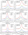 |
Fig. A.1. Parametric modelling of the most complex emission lines (from top to bottom, [Ar II], [Ne II], and [Ne III]) for the integrated spectra (R∼0.7″) both the N (left panels) and S (right panels) nucleus. The main part of the figure for all panels represent the original spectrum in black, the linear fit as the dashed, yellow line, and the total final modelling as the red line. The different Gaussian components are represented in green (primary), blue (secondary), and magenta (tertiary), when present. The rest-frame position is marked with a dashed, grey, vertical line at the corresponding wavelength in all panels. The bottom part of the figures show the residuals of the fit in black, with the 3σ limits as dashed, grey lines (see details in Sect. 2.2 and Hermosa Muñoz et al. 2024a). The velocity (corrected for the systemic value) and the velocity dispersion (corrected for the instrumental value) of every component are marked for each line. |
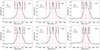 |
Fig. A.2. Non-parametric modelling for the integrated profiles of some ionised emission lines at different IP detected for the N nucleus assuming a radius of 0.7″. The flux has been normalised with the peak of the emission, and the wavelength has been transformed to velocity in km s−1 after redshift correction (see Sect. 1). In all panels the grey, dashed lines indicate the selected line limits, and the red, dashed lines mark the V02, V10, V50, V90 and V98 values (see Sect. 2). The labels indicate the line in each panel and the W80 parameter (see Sect. 2). |
All Tables
Flux measurements of the emission lines of NGC 6240 in the integrated spectra (r ∼ 0.7″) of both nuclei, ordered by ionisation potential.
All Figures
|
Fig. 1. False-colour images of NGC 6240 produced combining the MIRI images (see Sect. 2 for the details). Image a was obtained with the filters F560W and F1130W within an approximate FoV of 90″ × 90″ (1″ = 526 pc). Image b was obtained with the filters F770W and F1130W within an approximate FoV of 80″ × 80″ and the nuclei saturated to highlight the low-level structure. Panel c shows a zoom-in (approximate FoV of 7″ × 8″) to the F560W-filter image in logarithm scale with the position of the two radio sources in Gallimore & Beswick (2004) marked as blue crosses. The twelve contour levels in panel c go from 0.2% up to 73% of the flux peak, also in logarithm scale. We note that the diffraction spikes produced by the unresolved component of both nuclei have not been corrected. In all panels, north is up and east to the left. |
| In the text | |
|
Fig. 2. Total integrated spectra for the northern (dark blue) and southern (black) nuclei of NGC 6240 obtained with a circular aperture of radius 0.7″. The top panel shows the full MRS spectral range after scaling the flux of some individual bands to match between them. The middle and bottom panels show the spectra per channel, with the main ionised gas emission lines indicated in blue, the H2 rotational lines in yellow, and the recombination H I lines in green. The wavelength is in rest frame assuming a redshift of 0.02448 (see Sect. 2). We applied a residual fringe correction for the 1D extracted spectra in ch3 and ch4 (see Argyriou et al. 2023). |
| In the text | |
|
Fig. 3. Integrated profiles (r = 0.7″) of all the emission lines detected in the northern (upper panels) and southern (bottom panels) nucleus, after applying the fringing correction (see Sect. 2.1), normalised to the maximum flux. The lines are separated by IP, left IP < 25 eV, middle 25 < IP < 90 eV, and right IP > 90 eV. The rest-frame velocity corresponding to a z = 0.02448 is indicated with a dashed, grey, vertical line. We note that [O IV] is blended with [Fe II] at 25.99 μm and [Ne V] with [Cl II] at 14.37 μm (middle and right panels, see Sect. 3.1). We note that in the lower-right panel, [Ne VI] and [Mg V] are embedded in PAH features, and thus they are not detected in the original integrated spectrum (see Sects. 3 and 4.2). |
| In the text | |
|
Fig. 4. Kinematic maps obtained with the modelling of a single Gaussian for the [Ne II], [Ne III], and [Fe II] at 5.34 μm and Pfα lines (from top to bottom, respectively). The latter line kinematics were obtained after re-binning the cube with a 2 × 2 box (see Sect. 2.2). From left to right: flux in erg s−1 cm−2, velocity in km s−1, and velocity dispersion in km s−1. The contours in the velocity maps go from −300 to 300 km s−1 (increments of 100 km s−1). The contours in the flux maps go from 10−16 to 10−14 erg s−1 cm−2 (divided in 5 contours), except for Pfα (from 10−17 to 10−15 erg s−1 cm−2). White stars indicate the photometric centre for both nuclei in their corresponding sub-channels, and the lower-left line indicate the 1″ physical scale. The (0, 0) point in each panel marks the centre of the FoV at each channel. For all maps, north is up and east to the left. |
| In the text | |
|
Fig. 5. Kinematic maps obtained with the modelling of a single Gaussian for the [O IV], [Ne V], [Ne VI], and [Mg V] lines, top to bottom. A full description is in Fig. 4. |
| In the text | |
|
Fig. 6. Schematic figure of the main features seen in the flux and kinematic maps of the emission lines superimposed onto the [Ne III] flux map contours (see Fig. 4). In red we mark the position of the different detected clumps (namely C1, C2, and C3), and in green are the extended emission regions (namely Ext1 and Ext2, see Sect. 3.2). The bubble-like structure mainly detected with the high-excitation lines is in blue (extending up to ∼5.2″, i.e. 2.74 kpc; see Fig. 5 and Sect. 4.3), and the bridge detected between both nuclei (separated ∼1.6″, i.e. ∼840 pc; see Sect. 3.1) is marked in yellow. The purple regions indicate the V-shaped structure detected in the velocity dispersion maps. Additionally, we mark with black, dashed circles the region where we integrated the spectra for both nuclei, as well as their position with the white stars. |
| In the text | |
|
Fig. 7. Flux map of the PAH feature at 6.2 μm in log scale estimated after subtracting a local continuum from both sides of the feature. The contour levels go from 10−16 to 10−14 erg s−1 cm−2. |
| In the text | |
|
Fig. 8. Line ratios between [Ne III] and [Ne II] in log scale (upper panel) and [Fe II] over [Ar II] in linear scale (bottom panel). In the top panel we superimpose the contours from the [Ne III] flux map (see Fig. 4). The white stars indicate the position of both nuclei. |
| In the text | |
|
Fig. 9. Full integrated (r ∼ 0.7″) spectrum of the two nuclei in rest frame after modelling the dust features and continuum (see details in Sect. 4.2). The upper figures show the global fit to the S (top) and N (bottom) nucleus before (blue) and after (orange) subtracting the total PAH emission (black). The modelled contribution of the individual PAH features are shown in grey. The bottom panels show some insets near the region of [Mg V], Pfα, [Ne VI], and [Ne V] lines for both nuclei. The rest-frame wavelengths are indicated with a dashed, grey, vertical line. The Pfα and [Ne VI] lines from the S nucleus have been scaled for visualisation purposes. |
| In the text | |
|
Fig. 10. Mid-IR diagnostic diagram representing log([Ne V]/[Ne II]) versus log([Ne III]/[Ne II]) to divide between AGN (red area), shocks (green area), and SF (purple line) ionisation based on Fig. 5 in Feltre et al. (2023). The shaded areas schematically represent part of the grid of models in Feltre et al. (2023), and are used here just as a reference. We represent with a blue and a black star the position of the N and S nucleus, respectively (see Sect. 3.3). For comparison, we show the integrated value derived by Armus et al. (2006) for NGC 6240 as a white circle, and the nuclear values obtained with similar JWST data for other local type-2 Seyfert galaxies: yellow circle for NGC 7172 (Hermosa Muñoz et al. 2024b), orange circle for NGC 6552 (Álvarez-Márquez et al. 2023), dark (light) green triangles for the total (primary component) flux of the line for the type-1.5 Seyfert NGC 7469 (Armus et al. 2023), and red circle for NGC 7319 (Pereira-Santaella et al. 2022). Additionally, we show the ratios for two LINERs, namely NGC 4594 and NGC 1052, as a blue and brown squares, respectively (Goold et al. 2024). |
| In the text | |
|
Fig. A.1. Parametric modelling of the most complex emission lines (from top to bottom, [Ar II], [Ne II], and [Ne III]) for the integrated spectra (R∼0.7″) both the N (left panels) and S (right panels) nucleus. The main part of the figure for all panels represent the original spectrum in black, the linear fit as the dashed, yellow line, and the total final modelling as the red line. The different Gaussian components are represented in green (primary), blue (secondary), and magenta (tertiary), when present. The rest-frame position is marked with a dashed, grey, vertical line at the corresponding wavelength in all panels. The bottom part of the figures show the residuals of the fit in black, with the 3σ limits as dashed, grey lines (see details in Sect. 2.2 and Hermosa Muñoz et al. 2024a). The velocity (corrected for the systemic value) and the velocity dispersion (corrected for the instrumental value) of every component are marked for each line. |
| In the text | |
|
Fig. A.2. Non-parametric modelling for the integrated profiles of some ionised emission lines at different IP detected for the N nucleus assuming a radius of 0.7″. The flux has been normalised with the peak of the emission, and the wavelength has been transformed to velocity in km s−1 after redshift correction (see Sect. 1). In all panels the grey, dashed lines indicate the selected line limits, and the red, dashed lines mark the V02, V10, V50, V90 and V98 values (see Sect. 2). The labels indicate the line in each panel and the W80 parameter (see Sect. 2). |
| In the text | |
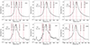 |
Fig. A.3. Same as Fig. A.2 but for the S nucleus. |
| In the text | |
Current usage metrics show cumulative count of Article Views (full-text article views including HTML views, PDF and ePub downloads, according to the available data) and Abstracts Views on Vision4Press platform.
Data correspond to usage on the plateform after 2015. The current usage metrics is available 48-96 hours after online publication and is updated daily on week days.
Initial download of the metrics may take a while.