| Issue |
A&A
Volume 690, October 2024
|
|
|---|---|---|
| Article Number | A95 | |
| Number of page(s) | 21 | |
| Section | Extragalactic astronomy | |
| DOI | https://doi.org/10.1051/0004-6361/202450071 | |
| Published online | 01 October 2024 | |
MICONIC: JWST/MIRI MRS observations of the nuclear and circumnuclear regions of Mrk 231
1
Centro de Astrobiología (CAB), CSIC-INTA, Camino Bajo del Castillo s/n, 28692 Villanueva de la Cañada, Madrid, Spain
2
Telespazio UK for the European Space Agency (ESA), ESAC, Camino Bajo del Castillo s/n, 28692 Villanueva de la Cañada, Spain
3
Sorbonne Université, CNRS, UMR 7095, Institut d’Astrophysique de Paris, 98bis bd Arago, 75014 Paris, France
4
Institut Universitaire de France, Ministère de l’Enseignement Supérieur et de la Recherche, 1 Rue Descartes, 75231 Paris Cedex 05, France
5
Leiden Observatory, Leiden University, PO Box 9513 2300 RA Leiden, The Netherlands
6
UK Astronomy Technology Centre, Royal Observatory, Blackford Hill, Edinburgh, EH9 3HJ Scotland, UK
7
Centro de Astrobiología (CAB), CSIC-INTA, Ctra. de Ajalvir km 4, Torrejón de Ardoz, 28850 Madrid, Spain
8
European Space Agency, c/o Space Telescope Science Institute, 3700 San Martin Drive, Baltimore, MD 21218, USA
9
I. Physikalisches Institut, Universität zu Köln, Zülpicher Str. 77, 50939 Köln, Germany
10
Max-Planck Institut für Radioastronomie (MPIfR), Auf dem Hügel 69, 53121 Bonn, Germany
11
Sterrenkundig Observatorium, Universiteit Gent, Krijgslaan 281 S9, 9000 Gent, Belgium
12
LESIA, Observatoire de Paris, Université PSL, CNRS, Sorbonne Université, Sorbonne Paris Citeé, 5 Place Jules Janssen, 92195 Meudon, France
13
Centre for Extragalactic Astronomy, Durham University, South Road, Durham DH1 3LE, UK
14
Department of Astronomy, Stockholm University, The Oskar Klein Centre, AlbaNova, 106 91 Stockholm, Sweden
15
Institute of Astronomy, KU Leuven, Celestijnenlaan 200D, 3001 Leuven, Belgium
16
Dept. of Astrophysics, University of Vienna, Türkenschanzstr. 17, 1180 Vienna, Austria
17
ETH Zürich, Institute for Particle Physics and Astrophysics, Wolfgang-Pauli-Str. 27, 8093 Zürich, Switzerland
18
Max Planck Institute for Astronomy, Konigstuhl 17, 69117 Heidelberg, Germany
19
Universite Paris-Saclay, Universite Paris Cite, CEA, CNRS, AIM, 91191 Gif-sur-Yvette, France
Received:
22
March
2024
Accepted:
27
June
2024
Abstract
We present JWST/MIRI MRS spatially resolved ∼5 − 28 μm observations of the central ∼4 − 8 kpc of the ultraluminous infrared galaxy and broad absorption line quasar Mrk 231. These are part of the Mid-Infrared Characterization of Nearby Iconic galaxy Centers (MICONIC) program of the MIRI European Consortium guaranteed time observations. No high excitation lines (i.e., [Mg V] at 5.61 μm or [Ne V] at 14.32 μm) typically associated with the presence of an active galactic nucleus (AGN) are detected in the nuclear region of Mrk 231. This is likely due to the intrinsically X-ray weak nature of its quasar. Some intermediate ionization potential lines, for instance, [Ar III] at 8.99 μm and [S IV] at 10.51 μm, are not detected either, even though they are clearly observed in a star-forming region ∼920 pc south-east of the AGN. Thus, the strong nuclear mid-infrared (mid-IR) continuum is also in part hampering the detection of faint lines in the nuclear region. The nuclear [Ne III]/[Ne II] line ratio is consistent with values observed in star-forming galaxies. Moreover, we resolve for the first time the nuclear starburst in the mid-IR low-excitation line emission (size of ∼400 pc, FWHM). Several pieces of evidence also indicate that it is partly obscured even at these wavelengths. At the AGN position, the ionized and warm molecular gas emission lines have modest widths (W80 ∼ 300 km s−1). There are, however, weak blueshifted wings reaching velocities v02 ≃ − 400 km s−1 in [Ne II]. The nuclear starburst is at the center of a large (∼8 kpc), massive rotating disk with widely-spread, low velocity outflows. Given the high star formation rate of Mrk 231, we speculate that part of the nuclear outflows and the large-scale non-circular motions observed in the mid-IR are driven by its powerful nuclear starburst.
Key words: galaxies: evolution / galaxies: ISM / galaxies: nuclei / quasars: general / quasars: individual: Mrk 231
Corresponding author; This email address is being protected from spambots. You need JavaScript enabled to view it. .
© The Authors 2024
 Open Access article, published by EDP Sciences, under the terms of the Creative Commons Attribution License (https://creativecommons.org/licenses/by/4.0), which permits unrestricted use, distribution, and reproduction in any medium, provided the original work is properly cited.
This article is published in open access under the Subscribe to Open model. This email address is being protected from spambots. You need JavaScript enabled to view it. to support open access publication.
1. Introduction
The InfraRed Astronomical Satellite (IRAS) discovered a large number of the important population of infrared (IR) bright galaxies, mostly in the local Universe. They were classified in terms of their IR (8 − 1000 μm) luminosities (LIR) as luminous and ultraluminous IR galaxies (LIRGs and ULIRGs) with LIR = 1011 − 1012 L⊙ and LIR = 1012 − 1013 L⊙, respectively. Follow-up observations revealed that a significant number of local ULIRGs are interacting and merger systems, are powered by intense star formation (SF) activity and/or an active galactic nucleus (AGN), and contain large amounts of molecular gas. It was also proposed that the dust-enshrouded ULIRG phase precedes the formation of quasars and eventually elliptical galaxies (see Sanders & Mirabel 1996, for a review). Sensitive mid-infrared (mid-IR) observations taken with the InfraRed Space Observatory (ISO) and the Spitzer Space Telescope provided diagnostic tools that allowed estimates of the AGN bolometric contribution to LIR and nuclear extinctions of local ULIRGs, among many other properties (see e.g., Genzel et al. 1998; Veilleux et al. 2009).
Mrk 231 (IRAS 12540+5708) is a ULIRG (log[LIR/L⊙]=12.5) and a broad absorption line (BAL) quasar (see e.g., Boksenberg et al. 1977; Lípari et al. 2005; Rupke et al. 2005, and references therein). It is also the nearest quasar, located at a redshift of z = 0.04217 that, following Feruglio et al. (2015), corresponds to a luminosity distance of D = 187.6 Mpc and an angular scale of 837 pc/″. It was recognized, more than fifty years ago, as an extraordinarily high IR luminosity source from ground-based 10 μm observations (Rieke & Low 1972), later confirmed by IRAS. Subsequent deep optical imaging demonstrated that Mrk 231 is an advanced merger (Sanders et al. 1987) or even a triple merger (Misquitta et al. 2024).
Emission from dust heated by both AGN and SF activity is responsible for its high IR luminosity, although estimates of the AGN bolometric contribution vary widely, from ≃30% to ≃70% (see e.g., Downes & Solomon 1998; Lonsdale et al. 2003; Veilleux et al. 2009; Yamada et al. 2023). Mrk 231 is also one of the best examples of a local quasar and ULIRG, where multi-phase (neutral, ionized, and molecular) and multi-scale outflows have been detected (Lipari et al. 2009; Fischer et al. 2010; Rupke & Veilleux 2011; Cicone et al. 2012; Feruglio et al. 2010, 2015; Aalto et al. 2012, 2015; Morganti et al. 2016; Veilleux et al. 2016; González-Alfonso et al. 2018; Misquitta et al. 2024). The velocities are typically of the order of hundreds of km s−1, although they reach velocities in excess of 1000 km s−1 in the neutral and molecular gas. These outflows are likely driven by both the AGN and the intense SF taking place in Mrk 231, although the high velocity outflow is likely AGN driven (see Rupke & Veilleux 2013, and references therein). Leighly et al. (2014) proposed a physical model for feedback from the AGN component, based on spectra ranging from the ultraviolet to the near-IR, and using the Paα line they estimated a black hole mass of 2.3 × 10⁸ M⊙.
Despite the presence of a quasar and the intense SF activity of Mrk 231, ISO and Spitzer spectroscopic observations revealed just a handful of mid-IR low-excitation emission lines and H2 transitions accompanied by a strong mid-IR continuum, but no high-excitation lines. Additionally, only a few polycyclic aromatic hydrocarbon (PAH) features with low equivalent widths (EW) were detected (see e.g., Genzel et al. 1998; Armus et al. 2007; Veilleux et al. 2009). Sub-arcsecond resolution mid-IR imaging, spectroscopy, and polarimetry with ground-based 8 − 10 m-class telescopes demonstrated that the emission is dominated by a bright, mostly unresolved, source (angular size of 0.1 − 0.4″ ≃ 84 − 330 pc), with a moderately deep 9.7 μm feature due to amorphous silicates (Soifer et al. 2000; Alonso-Herrero et al. 2016a,b; Lopez-Rodriguez et al. 2017). The ground-based observations also showed that the AGN accounts for a substantial fraction of the mid-IR continuum emission of Mrk 231, with only a small contribution from SF activity. The latter likely increases at longer wavelengths (see e.g., Efstathiou et al. 2022).
We present integral field unit (IFU) spectroscopy of Mrk 231 obtained with the Mid-Infrared Spectrometer (MRS) of the Mid-InfraRed Instrument (MIRI, Rieke et al. 2015; Wright et al. 2015, 2023) on board of the James Webb Space Telescope (JWST, Gardner et al. 2023). The observations are part of the guaranteed time observations (GTO) program termed Mid-Infrared Characterization of Nearby Iconic galaxy Centers (MICONIC) of the MIRI European Consortium, which includes Mrk 231, Arp 220, NGC 6240, Centaurus A, and SBS0335−052, as well as the region surrounding Sgr A* in our galaxy. These targets are also part of the GTO program for nearby galaxies of the NIRSpec instrument team. The goal of this work is to carry out a spatially resolved study of the mid-IR emission of the nuclear and circumnuclear regions of Mrk 231.
The paper is organized as follows. Section 2 describes the MRS observations, data reduction, and analysis, and Sect. 3 the mid-IR nuclear emission of Mrk 231. In Sects. 4 and 5 we analyze the spatially resolved observations of the ionized gas and warm molecular gas, respectively. In Sects. 6 and 7 we use these new spatially resolved MRS observations to infer the SF activity and outflow properties of this ULIRG. In Sect. 8 we present our summary.
2. MIRI MRS observations
2.1. Data reduction
We obtained MIRI MRS observations of the central region of Mrk 231, as part of JWST Cycle 1 program ID 1268 that also includes the NIRSpec GTO observations of this target. The MIRI observations were taken using a single pointing observed with a four-point dither, extended source pattern. The on-source integration was 522 s and made use of the FASTR1 readout mode. We also took an MRS background observation using a two-point dither, extended source pattern. The observations cover the full ∼5 − 28 μm spectral range.
We processed the MRS observations using version 1.12.3 of the JWST Science Calibration Pipeline (Bushouse et al. 2023)1, and the files from context 1135 of the Calibration References Data System (CRDS). We followed the standard procedure for MRS data (see Labiano et al. 2016; Álvarez-Márquez et al. 2023) for stages 1 and 2 of the pipeline. The first stage of the MRS pipeline (Morrison et al. 2023; Dicken et al. 2022) performs the detector-level and cosmic ray corrections, and transforms the ramps to slope detector images. The default cosmic ray correction and parameters did not leave any significant residuals in the data. The second stage performs the specific corrections needed for the MRS data (Argyriou et al. 2023; Gasman et al. 2023; Patapis et al. 2024).
At the end of stage 2, our data showed some negative spikes in the Level 2 science cubes. Investigation and discussion with STScI showed that these were caused by bad or warm pixels (flagged as NaN) in the detector, exactly atop the brightest part of the spectral traces. The negative residuals were the result of the pipeline interpolating these around using neighbouring pixels. At the time of our data reduction, we solved the problem by searching for isolated NaNs and interpolating in the spectral direction (D. Law, private communication) in the cal.fits. We note that currently the pipeline uses a pixel replacement routine to replace bad pixels flagged with a bad-pixel map. We then ran pipeline stage 3 on this modified datasets to combine the 4-dither pointings and create the final spectral cubes (Law et al. 2023). We switched off the background corrections (bkg_subtract and master_background) and sky matching (imatch) steps as they introduced artifacts. Although stage 3 is usually ran just on the science data, we also created Level 3 background cubes with the same procedure as the science cubes. These can be used to extract one-dimension (1D) background spectra to be compared to the science spectra.
We chose to produce the fully reconstructed science data cubes in the usual orientation of north up, and east to the left. The resulting fields of view (FoV) and pixel sizes are (see Fig. A.1 for a few examples): between 5.1″ × 5.6″ and 5.1″ × 5.9″ with a 0.13″ pixel size for channel 1 (ch1, observed wavelengths 4.9 − 7.65 μm), 6″ × 7″ and 6.3″ × 7″ with 0.17″ for channel 2 (ch2, 7.51 − 11.7 μm), 7.8″ × 8.6″ and 8.2″ × 8.6″ with 0.2″ for channel 3 (ch3, 11.55 − 17.98 μm), and 10.1″ × 10.9″ and 10.9″ × 10.9″ with 0.35″ for channel 4 (ch4, 17.7 − 27.9 μm). For reference, on the archival (proposal ID 10592) Hubble Space Telescope (HST) image of Fig. 1 taken with the Advanced Camera for Surveys (ACS), we overlaid the approximate FoV and orientation of the ch3 observations. These cover, apart from the nuclear region, some of the expanding shells and super-bubbles identified by Lípari et al. (2005), which are believed to be associated with the intense SF activity taking place in Mrk 231. We will discuss this in detail in Sects. 6 and 7.
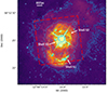 |
Fig. 1. Archival HST/ACS image (color and contours, shown in a square root scale) of Mrk 231. The observation was taken with the optical F435W filter and it shows the central 16″ × 16″, which corresponds to a region of ≃13.4 kpc × 13.4 kpc in size. For reference, the overlaid dashed square represents the approximate FoV and orientation of the MRS ch3 observations. We mark the positions of several expanding shells identified by Lípari et al. (2005) and discussed in the text. |
2.2. Data analysis
A bright nuclear point source dominates the mid-IR continuum emission in all the MRS channels (see some continuum maps in Fig. A.1), as already known from ground-based mid-IR observations at comparable angular resolutions (Soifer et al. 2000; Alonso-Herrero et al. 2016a; Lopez-Rodriguez et al. 2017). Indeed, the measured continuum full width at half maximum (FWHM) in all the MRS sub-channels is consistent with the reported values for point sources (Law et al. 2023; Argyriou et al. 2023), ranging in Mrk 231 from ∼0.3″ (251 pc) at 5 μm to ∼0.8 − 0.9″ at 23 μm (753 pc).
We extracted a 1D nuclear spectrum for each of the MRS sub-channels by centering a relatively large aperture of 1″ (≃837 pc) radius at the continuum peak. We chose it to encompass most of the extended nuclear line emission while avoiding emission from other circumnuclear star forming regions (see Sect. 4). Additionally, the large aperture size together with the four-point dither help minimize the continuum wiggles that are due to the undersampling of the point spread function (see Law et al. 2023). We applied the residual fringing correction to the nuclear 1D spectra in Fig. 2 with the RFC1D_UTILS routine2 (Kavanagh et al., in prep. and also Gasman et al. 2023). We did not apply an aperture correction to the nuclear 1D spectra because it contains both unresolved (continuum) and resolved (emission lines) components. We note that the aperture radius is large enough that the correction for the continuum unresolved emission would be less than approximately 10% for ch1 and ch2, but could reach 25% at the longest wavelengths (see Argyriou et al. 2023). For comparison we show the Spitzer/IRS spectra extracted as a point source in Fig. B.1. The flux calibration of the individual MRS channels was good and thus no correction factor was applied prior to the stitching of the sub-channels, except for ch1A for which needed to be multiplied by a 1.02 factor to match ch1B. Finally, given the extremely bright nuclear flux of Mrk 231, we did not perform a background subtraction since its contribution is negligible.
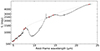 |
Fig. 2. MRS nuclear spectrum (solid black line) of Mrk 231. It was extracted with a 1″-radius aperture and covers the rest-frame ∼4.7 − 23.5 μm spectral range. We applied the residual fringing correction to the extracted 1D spectra of each of the sub-channels. The dotted line is the fitted continuum using a cubic spline function and the red dots are the anchor points selected for the fit. |
The resulting rest-frame ∼4.7 − 23.5 μm nuclear spectrum is shown in Fig. 2. We did not include ch4C because the red end is still affected by residual noise. Fig. 3 shows the same nuclear spectra but separately for each channel. We marked the positions of the pure rotational H2 S(8) to S(1) transitions and fine-structure lines as well as broad absorption features and PAHs features. We measured the fluxes and velocity dispersion of the emission lines from the nuclear 1D spectra before applying the residual fringing correction. We fit a single Gaussian function and a local continuum, and then computed the FWHM after correcting for the wavelength-dependent instrumental resolution provided by Argyriou et al. (2023). The uncertainties of the fluxes and line widths were calculated from the propagation of the errors of the fitted parameters. The fluxes and line widths are listed in Table 1. We did not include the H2 S(6) transition because it is strongly affected by an H2O absorption feature (Fig. 3, top left). We note, however, that most emission lines present weak wings, especially blueshifted. In Sect. 7.1 we will quantify them using a non-parametric method.
 |
Fig. 3. Nuclear spectrum shown for each of the MRS channels. As in Fig. 2, the extraction aperture had a 1″-radius. Each panel shows the A, B, and C sub-channels (ch1 upper left, ch2 upper right, ch3 lower left, and ch4 lower right), except for ch4 for which we only show A and B (see text). The dashed lines mark the detected low-excitation fine-structure emission lines (blue and green) and rotational H2 lines (orange). The loosely dotted lines are other relatively low IP lines not detected in the nuclear spectrum (see text for more details). Also labeled are the positions of PAHs, silicate features, and some molecular absorption bands. |
MRS fluxes measured in the nuclear (r = 1″) region of Mrk 231.
To produce spatially resolved maps of the fine-structure emission lines and bright rotational H2 lines, we fitted a single Gaussian function and a linear continuum on a spaxel-by-spaxel basis. We adopted a 3 × Ncont detection threshold at the peak of the line over the continuum, where Ncont is the standard deviation of the continuum adjacent to the line. With these fits, we produced maps of the line intensity, the mean-velocity field using the velocity corresponding to the peak of the line, and the velocity dispersion after correcting from instrumental resolution. We refer the reader to Hermosa Muñoz et al. (2024) for a complete description of the method used to construct the line maps. We discuss these maps in Sects. 4, and 5 for the ionized and molecular gas, respectively.
3. Nuclear emission
3.1. Continuum emission
The nuclear spectrum of Mrk 231 presents a strong and steeply rising mid-IR continuum (Fig. 2). It is mostly produced by the bright point source, which dominates the emission in all the MRS channels (see Fig. A.1). The MRS continuum fluxes in the ≃8 − 12 μm spectral range are similar to those reported from ground-based observations (Soifer et al. 2000; Alonso-Herrero et al. 2016a; Lopez-Rodriguez et al. 2017) at ≃0.3″ resolution.
The modeling of the nuclear near- and mid-IR emission of Mrk 231 done by Lopez-Rodriguez et al. (2017) showed that most of the MRS continuum emission would stem from the dusty molecular torus, although a powerful nuclear starburst was also required to reproduce the near and mid-IR emission (see also Sects. 4 and 6). Indeed, using OH megamaser observations, Klöckner et al. (2003) detected a 100 pc-radius torus, which appears to be warped with respect to the larger-scale disk. The expected size of the hot and warm dust emission dominating the mid-IR continuum is expected to be smaller than the torus physical size since it would mostly arise in its inner walls (e.g., Hönig 2019; Nikutta et al. 2021; Alonso-Herrero et al. 2021). Thus, the Mrk 231 torus would be unresolved, even at the best MRS angular resolution (≃0.3″ Argyriou et al. 2023).
3.2. Low excitation emission lines, rotational H2 lines, and PAH features
In contrast to other nearby AGN and (U)LIRGs observed with MRS (see e.g., Pereira-Santaella et al. 2022; Álvarez-Márquez et al. 2023; García-Bernete et al. 2022a, 2024a; Armus et al. 2023, and also van der Werf et al., in prep.; Hermosa Muñoz et al., in prep.), there are only a few emission lines with relatively low EW (Figs. 2 and 3) in the nuclear spectrum. The series of pure rotational 0–0 S(8) to S(1) H2 lines is clearly detected in the nuclear region of Mrk 231. It is also evident that only fine-structure emission lines with low ionization potentials (IPs), between 7.9 eV and 41 eV, are present (Table 1). On the other hand, [Ar III] at 8.99 μm and [S IV] at 10.51 μm (loosely dotted lines in the upper right panel of Fig. 3) with IPs of 28 and 35 eV, respectively, are not detected in the nuclear region of Mrk 231. We note, however, that these lines are present in a circumnuclear star-forming region (see Sect. 6.2). When compared with previous Spitzer/IRS spectroscopic observations (see Armus et al. 2007; Veilleux et al. 2009, and also Fig. B.1), [Fe II], [Ar II], [Ar III], [Ne III], and [S III], as well as the S(8) to S(4) H2 lines are new MRS detections in the (circum)nuclear region of Mrk 231.
The observed ratio of [Ne III]/[Ne II] = 0.12 (Table 1) is well within the typical values of star-forming galaxies (average of 0.17 ± 0.07), while local quasars present significant higher ratios (average of 2.0 ± 1.0), both values from Spitzer/IRS spectra (Pereira-Santaella et al. 2010a), Moreover, photoionization models for AGN radiation fields (see Feltre et al. 2023, and references therein) predict [Ne III] to [Ne II] ratios above the observed ratio in Mrk 231. Only radiation fields with steep UV continua, which are representative of low ionization nuclear emission-line regions (LINERs), would produce low [Ne III]/[Ne II] ratios (see Fig. 6 of Feltre et al. 2023). However, the nuclear optical line emission of Mrk 231 is classified as a Seyfert 1 galaxy (see Sanders et al. 1988, and references therein).
van der Werf et al. (2010) modeled the CO rotational ladder of Mrk 231 using a combination of a photodissociation region (PDR) and an X-ray dominated region (XDR), with the latter being responsible for the emission of the high-J CO transitions. Models including an XDR produce mostly [Ne II], while the [Ne III] emission would be partly suppressed (Pereira-Santaella et al. 2017). Therefore, the relatively low [Ne III]/[Ne II] ratios in the nuclear region could be due to AGN photoionization with a contribution from an XDR. van der Werf et al. (2010) predicted a radial size of the X-ray illuminated region of 160 pc from the Mrk 231 using the range of intrinsic X-ray luminosity given by Braito et al. (2004). We note that this putative XDR would have a size smaller than that of the resolved nuclear starburst obtained from the low-excitation [Ar II] and [Ne II] emission lines (see Sect. 4.1). However, we have limited spatial information about the nuclear distribution of the [Ne III] emission line (see Sect. 4.1 and Appendix C). Thus, we cannot conclusively determine the effects of a putative XDR of Mrk 231 on the observed nuclear mid-IR line ratios.
Emission from the 6.2 μm and the 11.3 μm PAH features is clearly seen in the nuclear region of Mrk 231, together with other fainter PAH features typically detected in PDRs (see e.g., in the Orion bar, Chown et al. 2024), such as those at 5.25 and 12.7 μm, and tentatively at 16.45 μm (see Donnan et al. 2023). The relatively low EW of the PAH features for the 6.2 and 11.3 μm (see Sect. 6.1 for the measurements) reflects the dominance of an AGN produced mid-IR continuum, even though the extracted nuclear spectrum covers a relatively large physical region (central ≃1.6 kpc, in diameter).
3.3. High-excitation emission lines
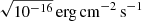
Mid-IR high-excitation lines with IP ≥ 95 eV (e.g., [Mg V] at 5.61 μm and [Ne V] at 14.32 μm) are generally associated with the presence of AGN (Sturm et al. 2002; Pereira-Santaella et al. 2022; García-Bernete et al. 2022a, 2024a; Armus et al. 2023; Álvarez-Márquez et al. 2023). Moreover, AGN present a good correlation between the [Ne V] at 14.32 μm luminosity, among several IR high excitation lines, and the intrinsic 2 − 10 keV luminosity (Spinoglio et al. 2022). These and other high-excitation lines remain undetected in the nuclear spectrum of Mrk 231 (see Fig. 3), despite the higher sensitivity and angular resolution of the MRS observations compared with previous observations (Armus et al. 2007; Veilleux et al. 2009). We can obtain an estimate of the line upper limits by measuring the standard deviation of the continuum (σcont) adjacent to the lines (see Fig. 4). For [Ne V] we corrected the 1D spectrum for residual fringing which was affecting the data at wavelengths mostly redder than the line. We note that for both lines, part of the continuum structure near the lines is due to the presence of individual absorption features (see Sect. 3.4). For the expected width of the [Mg V] and [Ne V] lines of Mrk 231, we took the FWHMline ≃ 700 km s−1 value measured by Rupke & Veilleux (2011) using the optical Hα line for the nuclear region, which they attributed to the nuclear wind. This value is higher than the measured FWHMline of the low excitation lines detected with MRS in Mrk 231 (Table 1), but these are produced mainly by SF activity (see Sect. 4). However, in NGC 7469 the broad components of [Ne V] and [Mg V] have FWHMline ≃ 726 − 814 km s−1 (Armus et al. 2023). The 3σcont upper limits are 1.1 × 10⁻¹⁴ erg cm−2 s−1 and 1.3 × 10⁻¹⁴ erg cm−2 s−1 for [Mg V] and [Ne V], respectively.
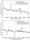 |
Fig. 4. Zoomed-in spectral regions of the nuclear spectra around the wavelengths of high-excitation lines [Mg V] (top) and [Ne V] (bottom). The black lines are the observed spectra extracted with an aperture radius of 0.5″ (top) and an aperture radius of 1″ (bottom), while the dotted and dashed lines are the predicted high-excitation emission lines from MRS observations of two local AGN assuming an intrinsic 2 − 10 keV luminosity of 1044 erg s−1 for Mrk 231 (see text for details). The ch3-medium spectrum was corrected for residual fringing that was affecting mostly data at wavelengths longer than that of [Ne V]. |
We can also use MRS observations of two AGN in local LIRGs to predict the expected fluxes of [Mg V] and [Ne V] for Mrk 231 using their X-ray luminosities. The intrinsic 2 − 10 keV luminosity of Mrk 231 was estimated to be between 2 × 1043 and ≃1044 erg s−1 (Braito et al. 2004, corrected for the distance assumed in this work), although other works (see e.g., Teng et al. 2014) inferred a lower value putting it in the intrinsically X-ray weak quasar category. Both the bright Seyfert 1 galaxy NGC 7469 (Armus et al. 2023) and the AGN in the northern nucleus of NGC 6240 (NGC 6240-N, Hermosa Muñoz et al., in prep.) present similar 2 − 10 keV luminosities, 3 × 1043 erg s−1 (Vasudevan et al. 2010) and 2 × 1043 erg s−1 (Puccetti et al. 2016), respectively.
We used the observed line fluxes of the high excitation lines in NGC 7469 (summing the narrow and broad components) and NGC 6240-N, scaled to the distance and a 2 − 10 keV luminosity of 1044 erg s−1 for Mrk 231 to predict the amplitudes of the two lines, assuming a single Gaussian function. Again we took FWHMline ≃ 700 km s−1. Figure 4 shows the simulated lines over spectra extracted with an aperture radius of 0.5″ for the [Mg V] line and 1″ for [Ne V]. The smaller aperture for ch1 is intended to minimize the continuum structure contribution near the line, while containing most of the unresolved emission at these wavelengths. The simulated [Mg V] lines are consistent with the non-detection in the observed spectrum, corresponding to a ≃1.7σcont detection, approximately. The [Ne V] line at 14.32 μm predicted from the NGC 7469 MRS flux would have been detected if the 2 − 10 keV luminosity of Mrk 231 was 1044 erg s−1 but would be undetected if Mrk 231 is an intrinsically X-ray weak quasar (Teng et al. 2014). On the other hand, the line flux predicted from NGC 6240-N would be buried within the noise and structure of the continuum emission. Therefore, the lack of detection of [Mg V] and [Ne V] in the nuclear region of Mrk 231 is likely due a combination of a strong mid-IR continuum, the presence of continuum structure due to absorption features, and its relatively weak X-ray emission (see also Teng et al. 2014).
3.4. Absorption features
The nuclear spectrum of Mrk 231 presents a ∼9.7 μm silicate feature in moderate absorption, as already known from ground-based observations with similar angular resolution (Alonso-Herrero et al. 2016a,b; Lopez-Rodriguez et al. 2017). A corresponding ∼18 μm feature was previously observed with Spitzer/IRS (Armus et al. 2007; Veilleux et al. 2009) at lower angular resolution. To measure the apparent optical depths of the silicate features, we fitted the continuum emission with a cubic spline function with several anchor points (red dots in Fig. 2 and continuum fit plotted as a dashed line). We calculated the apparent depths of the features as Sfeature = ln(ffeature/fcont) and obtained S9.7 μm = −0.75 and S18 μm = −0.24. These values are consistent with past observations, although they are subject to a precise extraction and fit of the continuum emission.
The high resolving power of MRS (Labiano et al. 2021; Jones et al. 2023; Argyriou et al. 2023) allows to identify numerous absorption features in Mrk 231. These include the previously detected features at ∼6.85 and 7.25 μm (Fig. 3), which are attributed to aliphatic hydrocarbons (possibly a:C–H hydrogenated amorphous carbon analogs, see Spoon et al. 2022, for more details), and at ≃13.7 μm and ≃14 μm produced by acetylene (C2H2) and hydrogen cyanide (HCN), respectively (Lahuis et al. 2007). Additionally, a newly detected absorption feature in Mrk 231 at 7.7 μm is due to methane (CH4) ice. All these absorption features are observed in the nuclear regions of other local (U)LIRGs (Rich et al. 2023; Buiten et al. 2024) and MICONIC targets (Buiten et al., in prep.; Hermosa Muñoz et al., in prep.).
Another remarkable finding is the large number of H2O rovibrational absorption lines in the 5.5 − 7.2 μm range (Fig. 3). These are associated with the gas phase of this molecule (González-Alfonso et al. 2024; García-Bernete et al. 2024b). Moreover, the H2O features of Mrk 231 appear to be similar to those of the embedded star-forming regions in the LIRG system VV 114 (Buiten et al. 2024). A strong mid-IR continuum source behind the absorbing gas is required to give rise to these features (González-Alfonso et al. 2024), which in the case of Mrk 231 is produced by dust heated by the AGN. Using Herschel observations González-Alfonso et al. (2010) detected far-IR water vapour features in absorption and emission and estimated the sizes of the regions where these features are formed to be at radii between 120 and 600 pc from the Mrk 231 nucleus. The latter basically corresponds to the extent of the nuclear starburst (see Sect. 4).
The nuclear spectrum of Mrk 231 also shows evidence of a broader and relatively shallow H2O feature at ∼6 μm, which is believed to be due to the presence of dirty water ices in obscured AGN and embedded nuclear regions of local ULIRGs (see García-Bernete et al. 2024a, and references therein). For the measured nuclear X-ray column density of Mrk 231 of 1.1 × 1023 cm−2 (Teng et al. 2014), according to García-Bernete et al. (2024a), the expected apparent optical depth of this ice feature would be small, which is consistent with the observations. A detailed modeling of this and other absorption features will be carried out in a future paper.
4. Extended ionized gas and PAH emission
In this section we discuss the properties of the extended ionized gas and PAH emission in Mrk 231. Figures 5 and 6 present maps of the line flux of the brightest fine-structure lines in Mrk 231 ([Ar II] and [Ne II] respectively) together with the mean-velocity field and velocity dispersion (left, middle, and right panels). In Figs. C.2 and C.3, we show similar maps for [Fe II], [Ne III], and [S III].
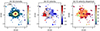 |
Fig. 5. Maps of [Ar II] at λrest = 6.99 μm. The maps were constructed by fitting a single Gaussian function and a local continuum to the emission line on a spaxel-by-spaxel basis. The panels show the intensity and contours in units of |
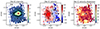 |
Fig. 6. Maps of [Ne II] at λrest = 12.81 μm. Panels and symbol are as in Fig. 5. The 0,0 point on the axes refers to the center of this sub-channel array, after rotation. In all maps, north is up and east to the left. |
4.1. Line flux maps
The intensity maps of the low-excitation emission lines exhibit not only bright emission arising in the nuclear region but also an extended emission component which includes several circumnuclear star-forming regions. This is in contrast to the bright point source present in the MRS continuum maps (see Fig. A.1). The location of a known star-forming region at approximately 1.1″ (920 pc) southeast (SE) of the AGN is detected in the [Ne II] and [Ne III] line maps (Figs. 6 and C.2), and is easily identified in the higher angular resolution map of [Ar II] (Fig. 5). The larger FoV of the [Ne II] maps also shows emission from another star-forming region located to the northeast (approximately 1″) of the AGN as well as some regions at ≃2.5 − 3″ (2.1 kpc) to the south (see Fig. C.6). These star-forming regions were previously detected in Mrk 231 using optical IFU observations (Lipari et al. 2009; Rupke & Veilleux 2011). They are related to the expanding shells S3 (at an approximate radial distance from the AGN of 1.2″) and S1 (at 3.5″ from the AGN), respectively (see Lípari et al. 2005; Lipari et al. 2009, and Fig. 1) and associated bright optical knots detected with HST (Surace et al. 1998, and also Fig. 1). We note that other works (see e.g., Surace et al. 1998; Rupke et al. 2005; Rupke & Veilleux 2011) described shell S1 as southern arc of star-forming regions and/or knots.
Interestingly, some of the bright circumnuclear star-forming regions in the MRS maps are identified by their relatively low values of the velocity dispersion (Figs. 5 and 6, right panels). As an example, the [Ar II] line from the region SE of the AGN has σ ≃ 40 km s−1 (corrected for instrumental resolution). Additionally, the [Ne II] intensity map shows more extended and diffuse emission3, which is associated with the overall interstellar medium of the galaxy, while the other more compact arisings in the star forming regions (see Sect. 7.2) .
From the [Ar II] and [Ne II] line flux maps, we measured the size of the nuclear region responsible for the low-excitation line emission. From spatial profiles extracted with 1″, we obtained nuclear sizes of 0.6 − 0.5″ (FWHM, 502 − 418 pc) along the east-west (E-W) and north-south (N-S) directions, respectively, for [Ar II] and slightly larger for [Ne II], 0.8 − 0.7″ (660 − 586 pc, FWHM). For the latter line we created an intensity map by integrating the line from a continuum-subtracted data cube. This is because the [Ne II] map created by fitting a single Gaussian (Fig. 6, left) contains some NaN in the central region which hamper the fit of the spatial cuts. For comparison, the derived sizes from spatial profiles taken from MRS continuum maps adjacent to the lines are 0.4 − 0.3″ along the E-W and N-S directions in ch1C and 0.6″ for ch3A. This indicates that a large fraction of the observed nuclear [Ar II] and [Ne II] emission is resolved.
It is likely that a contribution from unresolved emission is also present in the low excitation emission lines. The velocity channel maps of [Ne II] near the systemic velocity (Fig. D.1) show faint emission from the diffraction spikes associated with the unresolved source. Thus, a better estimate of the line emitting region can be obtained by subtracting in quadrature the FWHM of the core of the point spread function measured from the continuum images from the observed value. The resulting sizes for the [Ar II] and [Ne II] emissions are approximately 0.4 − 0.5″ = 335−420 pc (FWHM), respectively, for the nuclear line emission in both the E-W and N-S directions. These sizes are within the range observed in other local ULIRGs using ALMA sub-millimeter continuum observations (Pereira-Santaella et al. 2022) and similar to the values measured for the nuclear starburst of Mrk 231 with optical, near-IR, and radio observations (Lipari et al. 2009; Davies et al. 2004; Carilli et al. 1998). Therefore, both the mid-IR sizes and observed [Ne III]/[Ne II] ratio indicate that the MRS observations have resolved the nuclear starburst of Mrk 231.
4.2. Extended PAH emission
In galaxies, PAH molecules are excited by ultraviolet photons produced by B stars rather than the more massive O stars (see Peeters et al. 2004). Thus, PAH emission is often considered a tracer of the recent SF activity, while [Ne II] probes youngest ages (a few million years). We generated a map of the 11.3 μm PAH intensity by integrating, on a spaxel-by-spaxel basis, the observed feature flux between 11.6 μm and 11.95 μm (λrest = 11.13 μm and λrest = 11.47 μm) and subtracting a local continuum measured on both sides of the feature. We note that for Mrk 231 this feature lies close to the edge of the MRS ch3A (see bottom left panel of Fig. 3) and thus the local blue continuum might be slightly overestimated. The resulting map (Fig. 7, top panel) exhibits PAH emission over the entire ch3A FoV, with the brightest arising in the nuclear region. The detection of the 11.3 μm PAH feature in the central few hundred parsecs of Mrk 231 is in line with observations of the nuclear regions of other AGN with comparable X-ray luminosities (García-Bernete et al. 2022a, 2024c). These works showed that while the presence of an AGN can impact the properties of the PAH molecules, it does not necessarily destroy them completely.
 |
Fig. 7. Maps of the intensity of the 11.3 μm PAH feature (top) in units of 10−16 erg cm−2 s−1 and the 11.3 μm PAH to [Ne II] line ratio (bottom). The FoV and symbols are as in Fig. 6. The maps and contours are in a linear scale. |
Although the overall morphology of the 11.3 μm PAH feature emission is similar to [Ne II] (Fig. 6), some differences are apparent in the 11.3 μm PAH over [Ne II] line ratio map (Fig. 7, bottom). The nuclear region and some of the circumnuclear star-forming regions show distinctly lower ratios than in the rest of the extended emission. This behavior was observed in Spitzer/IRS spatially resolved line ratio maps of local LIRGs (Alonso-Herrero et al. 2009; Pereira-Santaella et al. 2010b). While the decreased 11.3 μm PAH/[Ne II] ratio in the nuclear region of Mrk 231 and LIRGs might be in part due to extinction due to silicate grains affecting the 11.3 μm PAH feature (Hernán-Caballero et al. 2020) and/or the AGN effects, they also reflect the fact that PAHs trace less massive and slightly older stellar populations than other mid-IR low excitation emission lines (Peeters et al. 2004). Nevertheless, the extended nature of the PAH and [Ne II] emissions reinforces the conclusion that most of the mid-IR low excitation line emission in Mrk 231 is produced by SF.
4.3. Ionized gas kinematics
The mean-velocity field of the [Ne II] line (middle panel of Fig. 6) shows evidence of circular motions, where the velocities vary from approximately −100 km s−1 to +80 km s−1. The isovelocity contours show that the kinematic major axis of the galaxy lies close to the E-W direction, as found by the kinematics of optical emission lines (Lipari et al. 2009) and the cold molecular gas (Downes & Solomon 1998; Feruglio et al. 2015). Moreover, the [Ne II] velocity field is similar to that derived from the optical Hα line (Lipari et al. 2009). This includes the presence of blueshifted motions to the south of the AGN at the location of star-forming regions associated with shell S1 (see Figs. 1 and C.6), where clearing of material and the possible rupture of a super-bubble are taking place (Lipari et al. 2009).
The higher angular resolution and spectral resolution view of the nuclear region provided by the [Ar II] line (middle panel of Fig. 5) shows a rotational pattern as well as non-circular motions in the central 2″ along the kinematic minor axis (N-S direction). These deviations from circular motions (see the expected velocity field for the rotating disk of Mrk 231 in the top left panel of Fig. 5 in Feruglio et al. 2015) are more pronounced in the warm molecular gas (see Sect. 5.2) as well as in the cold molecular gas (Feruglio et al. 2015). There are also some deviations from pure rotation in the [Ar II] and [Ne II] velocity fields at the location of the star-forming region ≃1.1″ SE of the AGN, which were also observed in Hα (Lipari et al. 2009; Rupke & Veilleux 2011). This might be related to the location of this star-forming region in the shell S3 (Lipari et al. 2009).
The velocity dispersion maps of [Ar II] and [Ne II] (right panels of Figs. 5 and 6, respectively) display moderate values (σ ∼ 60 − 120 km s−1) These are higher than the values measured in the star-forming regions discussed above, which have σ ∼ 30 − 40 km s−1 for the [Ar II] line or FWHMline ∼71 − 94 km s−1. These are similar to those measured from Hα (Rupke & Veilleux 2011). Although the lines are relatively narrow, the star-forming regions to the south might be located in areas of Mrk 231 affected by starburst-driven winds, as we shall see in Sect. 7.
5. Molecular hydrogen emission
In the nuclear region of Mrk 231 there is H2 emission from the S(1) to the S(8) transitions (see Fig. 2). In this section we discuss the morphology and kinematics of H2 S(1) and S(5), compute the mass and temperature of the warm molecular gas observed in the central region of Mrk 231. We note that the S(1) transition is present in both the ch3 and ch4 data cubes. In Appendix C, we show the ch3 S(2) and ch4 S(1) maps.
5.1. Line flux maps
The H2 S(5) line displays clearly extended emission in Mrk 231 (left panel of Fig. 8), as found for the low-excitation emission lines, with disk-like morphology. The emission confined to the approximately central ≃2″ region. It is resolved, with sizes of 0.75 − 0.6″ (FWHM ≃ 0.6 − 0.5 kpc) as measured from spatial cuts along the E-W and N-S directions, respectively. These are slightly larger than those of the [Ar II] and [Ne II] emitting region. There is H2 S(5) emission at the location of the star-forming region at 1.1″ SE of the AGN (Fig. 5), but it does not show a distinct peak there. The H2 S(5) morphology resembles that of the cold molecular gas disk traced with the CO(1−0) and CO(2−1) transitions as measured with millimetre interferometry (Bryant & Scoville 1996; Downes & Solomon 1998; Feruglio et al. 2015).
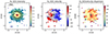 |
Fig. 8. Maps of H2 S(5) at λrest = 6.91 μm. Panels and symbol are as in Fig. 5. The 0,0 point on the axes refers to the center of this sub-channel array, after rotation. In all maps, north is up and east to the left. |
The H2 S(1) line emission (Fig. 9) fills almost entirely the ch3 FoV. The apparent deficit of emission at the central spaxels is due to the low contrast of the line against the strong continuum. The larger spaxel size of the ch4 H2 S(1) map (Fig. C.5) alleviates this problem showing that there is centrally peaked emission (FWHM ≃ 1 kpc) at the AGN position, as well as emission extending over ≃9″ × 9″ (projected size of 7.5 kpc × 7.5 kpc). It is thus more extended that the cold molecular gas disk (diameter of approximately 3″, Downes & Solomon 1998). However, it is likely that the large difference in sizes derived for the cold and warm molecular gas is because the more diffuse and extended cold molecular gas emission was filtered in the CO interferometric observations. The H2 S(1) morphology reveals additionally a spiral-like shape to the NE and SW, which appears to link with the central (∼30″) optical emission. The latter shows tidal tails extending toward the north and south on larger scales (> 1′, see Fig. 1 of Sanders et al. 1988).
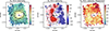 |
Fig. 9. Maps of H2 S(1) at λrest = 17.03 μm observed in ch3. Panels and symbol are as in Fig. 5. The 0,0 point on the axes refers to the center of this sub-channel array, after rotation. In all maps, north is up and east to the left. |
5.2. Warm molecular gas kinematics
The H2 S(5) mean-velocity field (middle panel of Fig. 8) shows a clear rotational signature consistent with a disk with a major axis oriented approximately in the E-W direction. The observed velocities are in the −80 km s−1 and +100 km s−1 range. There are, however, some deviations from circular motions along the kinematic minor axis with a marked inverted S-shaped pattern. The H2 S(5) velocity dispersions measured in the nuclear region are relatively low, σ ∼ 65 km s−1 (corrected for instrumental resolution), except along the kinematic minor axis mostly, where they reach slightly higher values. On larger scales, the H2 S(1) line present several regions with somewhat higher velocity dispersions (σ > 85 km s−1, right panel of Fig. 9). The H2 S(5) kinematics are remarkably similar to those of the interferometric CO(2−1) observations obtained at a ≃0.5″ resolution (compare with Fig. 4 of Feruglio et al. 2015, but note their smaller FoV). They modeled their observations with an inner disk of r = 0.12″ radius, which is warped with respect to the outer ring of radius r = 0.24″ with an E-W orientation and an inclination of 36°.
The kinematics of the H2 S(1) and (2) lines (Figs. 9, C.4, and C.5) connect well with those seen in the inner region traced by the S(5) line. The mean-velocity fields show qualitatively the same general E-W rotation pattern but with some interesting features indicating the presence of non-circular motions. There are redshifted features to the NE and SE, and blueshifted to the NW and SW. These are at projected radial distances from the AGN of approximately 2″ ≃1.5 kpc and might be related to expanding shells S2 (at an approximate radial distance from the AGN of 1.8″) and/or S3 (see Fig. 1), where the ionized gas shows outflow velocities between −500 km s−1 and −230 km s−1 (Lípari et al. 2005). The enhanced H2 velocity dispersions observed in some of these regions could be the result of the interaction between the ionized gas outflow and molecular gas in the galaxy. We analyse the molecular warm outflows in Sect. 7.
5.3. Warm molecular gas mass and temperature
In this section we use the suite of H2 pure rotational transitions (Table 1) detected in the nuclear region of Mrk 231 to estimate the warm molecular gas mass and temperatures. We note that the H2 ground S(0) transition is outside the ch4 spectral range, and thus we can only obtain a lower limit for the mass. For this analysis, we used the PDRTPY routine (Pound & Wolfire 2023), which fits a two-temperature model. We assumed local thermal equilibrium (LTE) conditions and a constant ortho-to-para ratio of 3 (see Álvarez-Márquez et al. 2023, for more details).
Using the observed H2 fluxes the temperatures are not well constrained, as can be seen from the top panel of Fig. 10. Both the S(3) and S(1) transitions are not well fitted with this model because they are located within the troughs of the 9.7 μm and 18 μm silicate feature absorptions, respectively (see Fig. 2). We tried values of the extinction around τ9.7 μm = 2, which are close to the extinctions derived by Veilleux et al. (2009) and Lopez-Rodriguez et al. (2017) (see also Sect. 6.1), and the regular Milky Way extinction law (see Hernán-Caballero et al. 2020) to derive extinction-corrected S(1), S(2), and S(3) line fluxes. A value of τ9.7 μm = 2.2 provided the smallest relative errors in the derived temperatures. As can be seen from Fig. 10 (bottom panel), the resulting fit to the excitation diagram is smoother. We note that this was not achieved if we corrected the fluxes with the lower extinction that would be derived from the apparent optical depths of the silicate features (Sect. 3). Moreover, compared with the diagram without an extinction correction, the temperatures are constrained significantly better, T1 = 519 ± 16 K and T2 = 1856 ± 110 K. For this fit, the derived total column density is higher, NH2 = 2.6 × 1020 cm−2. We note that in order to get a better determination of the extinction affecting the different emitting components in the nuclear region of Mrk 231, a more detailed modeling, including NIRSpec observations, would be necessary (see, e.g., Donnan et al. 2024).
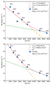 |
Fig. 10. H2 rotational diagrams for the nuclear region of Mrk 231. The fit was performed with a two-temperature model and assuming LTE conditions (see text for details). Top: using observed values and bottom: using the S(3), S(2), and S(1) fluxes corrected for extinction (see text for details). |
The corresponding warm (for the two temperatures fitted above) H2 mass is MH2(warm)=9 × 10⁶ M⊙ for r = 1″, from the fit with the extinction-corrected fluxes. Using Spitzer/IRS detected H2 transitions measured over larger physical sizes, Petric et al. (2018) estimated masses of warm molecular gas of ≃1.7 × 10⁸ M⊙ for the T = 106 K component and ≃3.1 × 10⁶ M⊙ for that at T = 343 K. Since Spitzer did not detect the S(4) to S(8) transitions, it is not surprising that these estimates did not include the higher temperature component detected in this work. Also, as expected, the MRS-derived mass is intermediate between the masses of hot molecular gas of 2.5 × 10⁴ M⊙ (Krabbe et al. 1997, for our assumed distance) derived from near-IR H2 lines and that of the cold molecular gas of 2.3 × 10⁹ M⊙ (Downes & Solomon 1998) derived from millimeter CO transitions.
6. Star formation activity
6.1. An obscured nuclear starburst
Several works in the literature inferred high values of the extinction in Mrk 231 from the modeling of the observed nuclear and integrated spectral energy distributions (i.e., τ9.7 μm = 2.23, AV = 36 ± 5 mag, and  , Veilleux et al. 2009; Lopez-Rodriguez et al. 2017; Efstathiou et al. 2022, respectively). Indeed, the H2 rotational diagram of the nuclear region derived with our MRS observations revealed that the S(1) and S(3) lines are affected by extinction (Sect. 5.3). In this section we discuss additional pieces of evidence to support this.
The comparison between the star formation rate (SFR) derived from LIR and some other mid-IR indicators can provide extra evidence for the presence of high levels of extinction. Since there are no detections of mid-IR hydrogen recombination lines in the nuclear region of Mrk 231, we can employ the [Ne II] and [Ne III] lines to estimate the SFR. With the calibration from Zhuang et al. (2019), which takes a Salpeter initial mass function, and assuming solar metallicity, we obtained a SFR ≃ 23 M⊙ yr−1 for the central 1.6 kpc. Integrating the neon lines over the entire ch3 FoV, we derived SFR ≃ 40 M⊙ yr−1. We note that if the metallicity of Mrk 231 is above solar, these estimates should be taken as upper limits. The neon-based SFR value is below several literature estimates (Carilli et al. 1998; Davies et al. 2004) and in particular that of ≃140 M⊙ yr−1 from LIR, once the AGN bolometric contribution (≃70%, Veilleux et al. 2009, 2020) is subtracted. This discrepancy thus could be resolved with a high value of the nuclear extinction.
The PAH emission can also provide additional clues considering that star-forming galaxies show relatively constant ratios between the EW of the 6.2, 11.3, and 12.7 μm PAH features. Using these, García-Bernete et al. (2022b) proposed a new method to identify deeply obscured nuclei since a decreased mid-IR continuum within the 9.7 μm silicate feature boosts the 11.3 μm PAH EW. This in turn produces lower EW(6.2 μm PAH)/EW(11.3 μm PAH) and EW(12.7 μm PAH)/EW(11.3 μm PAH) ratios. The main assumption here is that PAH emission is mostly produced in an extended component compared with the continuum source, as is the case in Mrk 231.
We measured nuclear EWs of the 6.2 μm, 11.3 μm, and 12.7 μm PAHs 0.007 ± 0.001 μm, 0.012 ± 0.001 μm, and 0.0005 ± 0.0001 μm, respectively4. The observed EW ratios, within the uncertainties, place the nuclear region of Mrk 231 within the region defined in the EW(6.2 μm PAH)/EW(11.3 μm PAH) versus EW(12.7 μm PAH)/EW(11.3 μm PAH) diagram (top panels of Fig. 8 of García-Bernete et al. 2022b) where deeply obscured nuclei are located. This is consistent with the detection of the HCN–vib (3−2) transition and the high nuclear column density of NH = 1.2 × 1024 cm−2 implied by these observations, which would be responsible for obscuring the mid-IR high-excitation emission lines (Aalto et al. 2015).
The deep silicate absorption features that would be arising in the most extinguished part of the nuclear starburst are, at the same time, partly filled in by the AGN dust continuum emission. In other words, the combination of both emissions produces the relatively low apparent optical depths of the silicates observed in the nuclear MRS spectrum (see Sect. 3). Therefore, the extinctions derived from the apparent depths need to be taken as lower limits to the true nuclear value.
6.2. Circumnuclear star-forming regions
The low-excitation fine-structure line maps have revealed the presence of several circumnuclear star-forming regions in Mrk 231 (Sect. 4 and Fig. C.6). That at ≃1.1″ SE of the AGN was detected and resolved in the ch1, ch2, and ch3 line maps (Figs. 5, 6, and C.2). In ch4A, this region is partially resolved (see the [S III] maps in Fig. C.3), since it is located slightly less than 2 × FWHMch4A from the AGN position. We placed a circular aperture of r = 0.3″ on the ch1, ch2, and ch3 data cubes to extract a 1D spectrum of this region. The size of the aperture encompasses well the region at the shortest wavelengths but the long wavelength continuum might be slightly contaminated by the bright AGN continuum source.
In Fig. 11 we show the rest-frame ch1 to ch3 spectra (top panel) and zoomed-in spectra (middle and bottom panels) around several fine-structure emission lines and H2 transitions. The 15 μm continuum of this star-forming region is more than a factor 50 fainter than the nuclear region and the lines present larger EW. Moreover, we detected two lines not identified in the nuclear spectrum, namely [Ar III] and [S IV], and tentatively the hydrogen recombination line H I 6−5 (Pfα) at λrest = 7.46 μm. The central rest-frame wavelengths in these panels, which were calculated with the nominal redshift of z = 0.04217, appear slightly redshifted as seen in the mean-velocity maps (Figs. 5 and 6, middle panels), due to rotation.
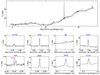 |
Fig. 11. MRS spectra of the star-forming region 1.1″ SE of the AGN. Top panel: ch1 to ch3 spectra extracted with a 0.3″ radius. We applied the residual fringing correction to the 1D spectra and scaling factors to stitch together the spectra of the different sub-channels. Middle and bottom panels: zoomed-in spectral regions of selected emission lines. In all panels, the rest-frame wavelengths were computed with the redshift quoted in Sect. 1 and appear redshifted with respect to the systemic velocity (see mean-velocity maps of [Ar II] and [Ne II], middle panels of Figs. 5 and 6), due to rotation. |
Using a single Gaussian function, we derived line ratios [Ne III]/[Ne II] ≃ 0.14 and [Ar III]/[Ar II] ≃ 0.22. The latter is likely just a lower limit since the [Ar III] line is inside the 9.7 μm silicate feature. Nevertheless, these ratios can be explained by photoionization models for relatively young (5 − 6 Myr) stellar populations formed in an instantaneous burst of solar metallicity with a Salpeter initial mass function and an upper mass cutoff of 100 M⊙ (Rigby & Rieke 2004).
In the star-forming regions to the south of the AGN, which are associated with the expanding shell S1, there is evidence of the presence of Wolf-Rayet stars (Lipari et al. 2009), indicating a young SF episode. We extracted a 1D spectrum from a region at 2.4″ south of the AGN with a radius of 0.8″. We measured [Ne III]/[Ne II] = 0.26, which is within the line ratios predicted for this stellar phase, again for a solar metallicity instantaneous burst (Rigby & Rieke 2004).
This brief analysis with the MRS observations reinforces the conclusions from Lipari et al. (2009) about the young ages of some of the circumnuclear star-forming regions in Mrk 231.
7. Ionized and warm molecular gas outflows
The outflows previously reported in Mrk 231 (see Sect. 1 for references and Veilleux et al. 2020, for a review) were observed in the nuclear region as well as up to a few kiloparsecs away from the AGN. Plausible explanations for their driving mechanism include the quasar, strong SF activity taking place in the galaxy, and/or the presence of a radio jet. This jet is observed in a nearly N-S direction but it is confined to the inner parsec. Since the mean-velocity fields of the low-excitation emission line and the H2 transitions present deviations from circular motions, on nuclear and circumnuclear scales (Sects. 4.3 and 5.2), in this section we analyze in detail the line profiles from the nuclear region and position–velocity (p–v) diagrams of the ionized and warm molecular gas in Mrk 231 to look for evidence of outflows.
7.1. Nuclear region
We constructed emission line profiles from the nuclear spectra (r = 1′′ aperture) after subtracting the fitted local continuum and normalizing them to the line peak. The [Fe II], [Ar II], and [Ne II] profiles (Fig. 12) show a similar overall shape with evidence of a weak blue wing (see below). The wings of the [Ne III] profile appear noisier due to the lower contrast of the line against the continuum. In general all the H2 lines (middle and right panels of Fig. 12) also show comparable shapes. Those with higher constrast over the continuum, namely, the S(5) and S(7) lines, present a blue wing as well.
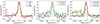 |
Fig. 12. Line profiles from the nuclear region (r = 1″ aperture). Left panel: fine-structure lines, and middle and right panels: H2 S(7) to S(4) and S(3) to S(1) transitions, respectively. The 0 km s−1 value corresponds to the adopted z = 0.004217. Note that the red part of the H2 S(6) line profile (green line, middle panel) is inside one of the H2O molecular absorptions. We did not apply the 1D residual fringe correction. |
The mid-IR line wings in Mrk 231 are not prominent and were not modeled with the single Gaussian fits in Sect. 2.2. To quantify their properties, we performed a non-parametric analysis with a similar method to that of Harrison et al. (2014). We computed the velocities at the 10th (v10) and 90th (v90) flux percentiles, the line width defined as W80 = abs(v90 − v10), as well as the velocities at the 2nd and 98th percentiles (v02 and v98, respectively). The largest of these two values provides an estimate of the maximum projected velocity of the outflow. We restricted this analysis to those lines with the highest contrast against the continuum, which are [Fe II], [Ar II], [Ne II], and the H2 S(7), S(5), and S(4). Appendix E provides details on the method and Fig. E.1 presents two examples of the line analysis.
All lines show similar widths ( ). The larger W80 with respect to the FWHMline from the single Gaussian fit (Table 1) are not solely due to the instrumental broadening, which has FWHM ∼ 100 km s−1 for [Ne II] (Argyriou et al. 2023). The velocities (Table 2) also revealed the presence of blueshifted wings being more extended in velocity, with [Ne II] presenting the largest blueshifted velocities, reaching
 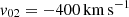 (Fig. E.1, left panel). Using two Gaussians, we fitted this line with a narrow component with FWHM
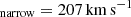 and a blueshifted (by approximately Δv = 97 km s−1) broad component with FWHM
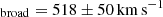 . An estimate of the maximum outflow velocity can be computed as vmax = Δv + 2 × σbroad (Fiore et al. 2017), which results in
 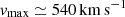 in the nuclear region of Mrk 231.
Non-parametric analysis of nuclear emission lines.
Additionally, the [Ne II] velocity channel maps also reveal that the nuclear blueshifted component is slightly more prominent than the redshifted one (see Fig. D.1). We note that the nuclear mid-IR emission of Mrk 231 is dominated by an extremely bright point source, which makes it challenging to separate out faint line wings from the residual continuum wiggles. In the case of [Ne II], which is the line with the highest signal-to-noise ratio, the presence of the 12.7 μm PAH feature limits the detection of an even more blueshifted line component, if present.
Since the observed nuclear [Ne II] emission in Mrk 231 is predominantly produced by SF (Sects. 3.2 and 6), the stronger blue wings in the lines could be produced in a starburst-driven outflow emerging perpendicular to the nearly face-on nuclear disk. However, we cannot rule out that it is associated with that detected in the nuclear optical emission lines with faster velocities (v = −1000 to −750 km s−1, Lipari et al. 1994; Rupke & Veilleux 2011). According to the latter work, the highest velocity component might be related to the AGN. We did not detect high velocities (|v|> 400 km s−1) in the warm molecular gas, which are present in CO(2−1) and CO(3−2) toward the NE and SW, on sub-arcsecond scales (Feruglio et al. 2015). These authors explained these motions due to the presence of two molecular outflows, an isotropic one and a wide-angle biconical outflow oriented in the NE to SW directions. It is again possible that the high velocity motions of the molecular gas are not detected due to the large extinction that is affecting the nuclear region in the mid-IR (Sect. 5).
Summarizing, we favor a scenario where the nuclear outflows observed in the mid-IR lines of Mrk 231 are driven by the powerful starburst. However, we cannot rule out an AGN origin of and/or contribution to these mid-IR outflows. For instance, some nearby Seyfert galaxies with evidence of AGN-driven outflows show relatively modest mid-IR line widths in their nuclear regions ( , see Hermosa Muñoz et al. 2024; Zhang et al. 2024). It is also clear that the exceptionally high velocities (≃1000 km s−1) detected in the neutral gas phase of Mrk 231 and extending in all directions from the center up to at least 2 kpc (Rupke & Veilleux 2011) would put a starburst-driven wind origin to its limits. Indeed, based on these observations (Rupke & Veilleux 2013) argued that the nuclear outflow is powered by the AGN (see also Leighly et al. 2014), and the coupling between the nuclear wind and the radio-jet might be responsible for accelerating the neutral gas to these high velocities (see also Rupke & Veilleux 2011).
7.2. Circumnuclear region
To investigate the presence of outflows outside the nuclear region, where the instrumental effects due to the bright central point source are diminished, we generated p–v diagrams along the kinematic minor axis (N-S direction) from the data cubes of the fine-structure lines [Ar II] and [Ne II], and the H2 S(5) and S(1) transitions. To do so, we placed a pseudo slit of 2′′ width (as the diameter of the aperture used to extract the nuclear 1D spectrum) on the portion of the data cube containing the line after subtracting a local linear continuum. At the AGN position, all four p–v diagrams (Figs. 13 and 14) show residuals, which are due to the bright point source wiggles, left after the continuum subtraction. In the case of the H2 S(1) line, residual fringes are also seen along the velocity (i.e., wavelength) axis.
 |
Fig. 13. Kinematic minor axis p–v diagrams for [Ar II] (left) and [Ne II] (right). The extraction aperture is 2′′. The 0,0 point in the spatial direction marks the AGN position. The first contour is drawn at three times the standard deviation of the (zero) continuum level. The position of the main expanding shells (Lípari et al. 2005) are marked as horizontal lines. In the right panel the vertical lines denote the estimated virial range. |
 |
Fig. 14. Kinematic minor axis p–v diagrams for H2 S(5) (left) and H2 S(1) (right) emission lines. Lines and symbols as Fig. 13. |
In the nuclear region of Mrk 231, the kinematic minor axis p–v diagrams of the fine structure lines (Fig. 13) show velocities from ≃ − 300 to +300 km s−1, and possibly to even higher blueshifted velocities in [Ne II]. However, it is also clear that the high values can also be due (in part) to the imperfect continuum subtraction done on a spaxel-by-spaxel basis. Moving away from the AGN continuum residuals at projected distances larger than 0.5 − 1′′, the ionized gas exhibits velocities centered at the systemic value (v = 0 km s−1 in these diagrams). The [Ne II] p–v diagram shows clearly the emission from the star-forming region(s) located ≃3′′ the south of the AGN, while the [Ar II] p–v diagram also reveals the star-forming region ≃1′′ north of the AGN. There is, however, another underlying, extended, and relatively broad component (see below).
Out to the location of shell S3, at a projected distance of ≃1.5′′ = 1.3 kpc from the AGN, the kinematic minor axis p–v diagram of the H2 S(5) line (left panel of Fig. 14) shows a tendency for redshifted velocities to the south and blueshifted velocities to the north. The velocities reach only a few hundred km s−1 and are also detected in the lower angular resolution p–v diagram of the H2 S(1) transition (right panel of Fig. 14). A comparable behavior was observed in the near-IR line 2.12 μm line on physical scales even closer to the AGN (Davies et al. 2004). There are some similarities between the H2 S(5) kinematic minor axis p–v diagram and those of the CO(2−1) transition (see middle panel of Fig. 7 of Feruglio et al. 2015). However, CO(2−1) shows redshifted velocities in excess 500 km s−1 in the nuclear region that are not observed in this H2 line. In the innermost region of Mrk 231, these deviations from rotation in the hot and cold molecular gas kinematics have been attributed to a warp of the inner disk (Davies et al. 2004; Feruglio et al. 2015). They could also indicate the presence of a molecular outflow in the disk of the galaxy.
On larger scales, at projected distances of a few arcseconds (several kpc) from the AGN, the H2 S(1) and [Ne II] minor axis p–v diagrams (right panels of Figs. 13 and 14) show a range of velocities. At ≃2′′ (≃1.6 kpc) of the AGN, they go from approximately ≃ − 200 to −300 km s−1 to ≃ + 200 to +300 km s−1. Following García-Burillo et al. (2015), we estimated a virial range of ±100 km s−1 for Mrk 231, by adding the contributions from turbulence as half the FWHM of the narrow component of [Ne II] in the southern star-forming region (observed FWHM = 130 − 135 km s−1), and in-plane non-circular motions approximated as 1/2 × vrot, where the (projected) rotation velocity is  (Downes & Solomon 1998). We can conclude that the MRS high velocities on these scales are not likely be attributed to the expected virial range of the rotating disk and could be related to extended outflows and/or expanding shells.
8. Summary
We presented JWST/MIRI MRS 4.9 − 27.9 μm observations of the ULIRG and BAL quasar Mrk 231 covering the central ≃5′′ × 6′′ (4.2 kpc × 5 kpc) in ch1 to ≃11′′ × 11′′ (9.2 kpc × 9.2 kpc) in ch4. The observations are part of the MIRI European Consortium GTO program MICONIC. Our main results are summarized as follows and in the cartoon of Fig. 15.
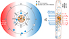 |
Fig. 15. Cartoon summarizing the different regions (not drawn to scale) of Mrk 231 identified with the MRS observations and other literature results. Left: front view, that is, in the plane of the sky, where the molecular gas disk is seen close to face-on. Right: side view to emphasize the possible scenario to explain some of the observed non-circular motions in the ionized and warm molecular gas. |
-
High excitation (IP ≥ 95 eV) emission lines, such as [Mg V] and [Ne V], remain undetected in these new and sensitive MRS observations. This is likely due to a combination of the X-ray weak nature and the bright mid-IR continuum emission of Mrk 231. The mid-IR evidence for the presence of an AGN comes from the bright unresolved nuclear continuum and low EW of PAH features. This bright continuum likely prevents the detection of [Ar III] and [S IV] (IP of 28 and 35 eV, respectively) in the nuclear region, whereas they are clearly observed in a star-forming region ≃920 pc SE from the AGN position.
-
A bright nuclear starburst with a size of ≃400 pc (FWHM) is resolved for the first time in the mid-IR in the [Ne II] and [Ar II] lines as well as rotational H2 transitions and PAH emission. The starburst extent is consistent with estimates derived at other wavelengths (Carilli et al. 1998; Davies et al. 2004). The low [Ne III]/[Ne II] ratio measured in the nuclear region is more typical of star-forming galaxies than AGN. Numerous absorption features associated with the gas-phase of water are present in the ∼5 − 7 μm spectral range. Assuming that they have similar origin as the water features observed in the far-IR, then they are formed within the nuclear starburst (González-Alfonso et al. 2010). All this supports the scenario where most of the mid-IR low-excitation line emission in the central region of Mrk 231 is produced by SF activity.
-
Several pieces of evidence, including the neon-based SFR, EW of PAH features, and the H2 excitation diagram, indicate that the nuclear starburst in Mrk 231 is partly obscured, even in the mid-IR. The extinction is higher than what would be derived from the apparent depth of the 9.7 μm silicate feature (S9.7 μm = −0.75), because it is partly filled in by the strong mid-IR continuum produced by the AGN.
-
Using the H2 S(1) to S(8) transition fluxes corrected for extinction, we estimated a mass of warm molecular gas in the central ≃1.7 kpc of 9 × 10⁶ M⊙ which is between the hot and cold molecular gas masses (Downes & Solomon 1998; Krabbe et al. 1997).
-
The nuclear line profiles show weak wings, which reach velocities of up to
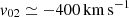 in [Ne II]. We interpreted these blueshifted velocities, as produced by a starburst-driven outflow. The more prominent blueshifted wings can be explained if the outflow is driven by the nearly face-on nuclear starburst. Similar blueshifted components are identified from optical observations, although with higher velocities (Lipari et al. 2009; Rupke & Veilleux 2011). We note however that the MRS observations cannot rule out an AGN origin for the nuclear outflow. Regardless of its origin, the lack of high velocity components and redshifted wings in the mid-IR lines could be due to a combination of a strong mid-IR continuum and obscuration.
 -
The extended [Ne II], H2 S(1), and 11.3 μm PAH emissions trace the ionized and warm molecular gas phases of the large-scale disk of Mrk 231 over the entire mapped region of ≃5 − 8 kpc. We detected several star-forming regions and complexes located up to a few kpc away from the AGN, which were already known from previous observations (Surace et al. 1998; Lipari et al. 2009; Rupke & Veilleux 2011). The emission from these regions is superimposed on a more extended and diffuse component.
-
The large-scale kinematics of the ionized and warm molecular gas show circular motions in a disk oriented in the approximate E-W direction, similar to that detected in cold molecular gas (Downes & Solomon 1998; Feruglio et al. 2015). There are also some deviations from rotation, seen as blue- and red-shifted motions with respect to the systemic velocity in the ≃200 − 300 km s−1 range. These non-circular motions are likely connected with the expanding shells and super-bubbles identified from optical imaging and IFU observations (Lipari et al. 2009) and/or the isotropic cold molecular gas outflow (Feruglio et al. 2015).
Summarizing, the unprecedented combination of sensitivity, high angular resolution, and spectral resolving power together with the broad spectral coverage afforded by MIRI MRS has enabled, for the first time, a detailed, spatially resolved study of Mrk 231 in the mid-IR. The picture that emerges is that a large fraction of the mid-IR line emission is produced in a spatially resolved powerful and obscured nuclear starburst. It is located in the central regions of a large (∼8 kpc) and massive and rotating disk where circumnuclear SF regions and widely-spread (low velocity) outflows in both the ionized and molecular gas are present. The Mrk 231 AGN reveals itself as a bright mid-IR continuum which, at the same time, might prevent the detection of relatively faint high-excitation lines produced by this X-ray weak quasar.
See also https://jwst-docs.stsci.edu/jwst-science-calibration-pipeline-overview
This is because [Ne II] is brighter than [Ar II] and the ch3 pixels are larger than those of ch1, thus making it easier to detect extended diffuse emission in [Ne II].
The uncertainties are driven by the continuum placement since the 6.2 and 11.3 μm PAH features are close to the edge of their corresponding sub-channel and the continuum red-wards the 12.7 μm feature is affected by the [Ne II] line wing (see Sect. 7.1).
Acknowledgments
We thank the anonymous referee for comments that helped improve the manuscript. We are grateful to I. García-Bernete, M. Pereira-Santaella, S. García-Burillo, and F. Donnan for insightful discussions about the MRS observations and scientific interpretation. AAH and LHM acknowledge support from grant PID2021-124665NB-I00 funded by the Spanish Ministry of Science and Innovation and the State Agency of Research MCIN/AEI/10.13039/501100011033 and ERDF A way of making Europe. MB acknowledges funding from the Belgian Science Policy Office (BELSPO) through the PRODEX project “JWST/MIRI Science exploitation” (C4000142239). JAM and LC acknowledge support by grant PIB2021-127718NB-100 from the Spanish Ministry of Science and Innovation/State Agency of Research MCIN/AEI/10.13039/50110001103. GÖ acknowledges support from the Swedish National Space Administration (SNSA). MJW acknowledges support from a Leverhulme Emeritus Fellowship, EM-2021-064. MIRI draws on the scientific and technical expertise of the following organisations: Ames Research Center, USA; Airbus Defence and Space, UK; CEA-Irfu, Saclay, France; Centre Spatial de Liége, Belgium; Consejo Superior de Investigaciones Científicas, Spain; Carl Zeiss Optronics, Germany; Chalmers University of Technology, Sweden; Danish Space Research Institute, Denmark; Dublin Institute for Advanced Studies, Ireland; European Space Agency, Netherlands; ETCA, Belgium; ETH Zurich, Switzerland; Goddard Space Flight Center, USA; Institute d’Astrophysique Spatiale, France; Instituto Nacional de Técnica Aeroespacial, Spain; Institute for Astronomy, Edinburgh, UK; Jet Propulsion Laboratory, USA; Laboratoire d’Astrophysique de Marseille (LAM), France; Leiden University, Netherlands; Lockheed Advanced Technology Center (USA); NOVA OptIR group at Dwingeloo, Netherlands; Northrop Grumman, USA; Max-Planck Institut für Astronomie (MPIA), Heidelberg, Germany; Laboratoire d’Etudes Spatiales et d’Instrumentation en Astrophysique (LESIA), France; Paul Scherrer Institut, Switzerland; Raytheon Vision Systems, USA; RUAG Aerospace, Switzerland; Rutherford Appleton Laboratory (RAL Space), UK; Space Telescope Science Institute, USA; Toegepast- Natuurwetenschappelijk Onderzoek (TNO-TPD), Netherlands; UK Astronomy Technology Centre, UK; University College London, UK; University of Amsterdam, Netherlands; University of Arizona, USA; University of Cardiff, UK; University of Cologne, Germany; University of Ghent; University of Groningen, Netherlands; University of Leicester, UK; University of Leuven, Belgium; University of Stockholm, Sweden; Utah State University, USA. A portion of this work was carried out at the Jet Propulsion Laboratory, California Institute of Technology, under a contract with the National Aeronautics and Space Administration. We would like to thank the following National and International Funding Agencies for their support of the MIRI development: NASA; ESA; Belgian Science Policy Office; Centre Nationale D’Etudes Spatiales (CNES); Danish National Space Centre; Deutsches Zentrum fur Luft-und Raumfahrt (DLR); Enterprise Ireland; Ministerio De Economía y Competitividad; Netherlands Research School for Astronomy (NOVA); Netherlands Organisation for Scientific Research (NWO); Science and Technology Facilities Council; Swiss Space Office; Swedish National Space Board; UK Space Agency. This work is based on observations made with the NASA/ESA/CSA James Webb Space Telescope. The data were obtained from the Mikulski Archive for Space Telescopes at the Space Telescope Science Institute, which is operated by the Association of Universities for Research in Astronomy, Inc., under NASA contract NAS 5-03127 for JWST; and from the European JWST archive (eJWST) operated by the ESDC. This research has made use of the NASA/IPAC Extragalactic Database (NED), which is operated by the Jet Propulsion Laboratory, California Institute of Technology, under contract with the National Aeronautics and Space Administration. This research made use of NumPy (Harris et al. 2020), Matplotlib (Hunter 2007) and Astropy (Astropy Collaboration 2013, 2018).
References
- Aalto, S., Garcia-Burillo, S., Muller, S., et al. 2012, A&A, 537, A44 [NASA ADS] [CrossRef] [EDP Sciences] [Google Scholar]
- Aalto, S., Garcia-Burillo, S., Muller, S., et al. 2015, A&A, 574, A85 [NASA ADS] [CrossRef] [EDP Sciences] [Google Scholar]
- Alonso-Herrero, A., Rieke, G. H., Colina, L., et al. 2009, ApJ, 697, 660 [NASA ADS] [CrossRef] [Google Scholar]
- Alonso-Herrero, A., Esquej, P., Roche, P. F., et al. 2016a, MNRAS, 455, 563 [NASA ADS] [CrossRef] [Google Scholar]
- Alonso-Herrero, A., Poulton, R., Roche, P. F., et al. 2016b, MNRAS, 463, 2405 [NASA ADS] [CrossRef] [Google Scholar]
- Alonso-Herrero, A., García-Burillo, S., Hönig, S. F., et al. 2021, A&A, 652, A99 [NASA ADS] [CrossRef] [EDP Sciences] [Google Scholar]
- Álvarez-Márquez, J., Labiano, A., Guillard, P., et al. 2023, A&A, 672, A108 [NASA ADS] [CrossRef] [EDP Sciences] [Google Scholar]
- Argyriou, I., Glasse, A., Law, D. R., et al. 2023, A&A, 675, A111 [NASA ADS] [CrossRef] [EDP Sciences] [Google Scholar]
- Armus, L., Charmandaris, V., Bernard-Salas, J., et al. 2007, ApJ, 656, 148 [NASA ADS] [CrossRef] [Google Scholar]
- Armus, L., Lai, T., U, V., et al. 2023, ApJ, 942, L37 [NASA ADS] [CrossRef] [Google Scholar]
- Astropy Collaboration (Robitaille, T. P., et al.) 2013, A&A, 558, A33 [NASA ADS] [CrossRef] [EDP Sciences] [Google Scholar]
- Astropy Collaboration (Price-Whelan, A. M., et al.) 2018, AJ, 156, 123 [Google Scholar]
- Boksenberg, A., Carswell, R. F., Allen, D. A., et al. 1977, MNRAS, 178, 451 [NASA ADS] [Google Scholar]
- Braito, V., Della Ceca, R., Piconcelli, E., et al. 2004, A&A, 420, 79 [NASA ADS] [CrossRef] [EDP Sciences] [Google Scholar]
- Bryant, P. M., & Scoville, N. Z. 1996, ApJ, 457, 678 [NASA ADS] [CrossRef] [Google Scholar]
- Buiten, V. A., van der Werf, P. P., Viti, S., et al. 2024, ApJ, 966, 166 [NASA ADS] [CrossRef] [Google Scholar]
- Bushouse, H., Eisenhamer, J., Dencheva, N., et al. 2023, https://doi.org/10.5281/zenodo.8404029 [Google Scholar]
- Carilli, C. L., Wrobel, J. M., & Ulvestad, J. S. 1998, AJ, 115, 928 [NASA ADS] [CrossRef] [Google Scholar]
- Chown, R., Sidhu, A., Peeters, E., et al. 2024, A&A, 685, A75 [NASA ADS] [CrossRef] [EDP Sciences] [Google Scholar]
- Cicone, C., Feruglio, C., Maiolino, R., et al. 2012, A&A, 543, A99 [NASA ADS] [CrossRef] [EDP Sciences] [Google Scholar]
- Davies, R. I., Tacconi, L. J., & Genzel, R. 2004, ApJ, 613, 781 [NASA ADS] [CrossRef] [Google Scholar]
- Dicken, D., Rieke, G., Ressler, M., et al. 2022, SPIE Conf. Ser., 12180, 121802R [NASA ADS] [Google Scholar]
- Donnan, F. R., García-Bernete, I., Rigopoulou, D., et al. 2023, MNRAS, 519, 3691 [CrossRef] [Google Scholar]
- Donnan, F. R., García-Bernete, I., Rigopoulou, D., et al. 2024, MNRAS, 529, 1386 [NASA ADS] [CrossRef] [Google Scholar]
- Downes, D., & Solomon, P. M. 1998, ApJ, 507, 615 [NASA ADS] [CrossRef] [Google Scholar]
- Efstathiou, A., Farrah, D., Afonso, J., et al. 2022, MNRAS, 512, 5183 [NASA ADS] [CrossRef] [Google Scholar]
- Feltre, A., Gruppioni, C., Marchetti, L., et al. 2023, A&A, 675, A74 [NASA ADS] [CrossRef] [EDP Sciences] [Google Scholar]
- Feruglio, C., Maiolino, R., Piconcelli, E., et al. 2010, A&A, 518, L155 [NASA ADS] [CrossRef] [EDP Sciences] [Google Scholar]
- Feruglio, C., Fiore, F., Carniani, S., et al. 2015, A&A, 583, A99 [NASA ADS] [CrossRef] [EDP Sciences] [Google Scholar]
- Fiore, F., Feruglio, C., Shankar, F., et al. 2017, A&A, 601, A143 [NASA ADS] [CrossRef] [EDP Sciences] [Google Scholar]
- Fischer, J., Sturm, E., González-Alfonso, E., et al. 2010, A&A, 518, L41 [NASA ADS] [CrossRef] [EDP Sciences] [Google Scholar]
- García-Bernete, I., Rigopoulou, D., Alonso-Herrero, A., et al. 2022a, A&A, 666, L5 [NASA ADS] [CrossRef] [EDP Sciences] [Google Scholar]
- García-Bernete, I., Rigopoulou, D., Aalto, S., et al. 2022b, A&A, 663, A46 [NASA ADS] [CrossRef] [EDP Sciences] [Google Scholar]
- García-Bernete, I., Alonso-Herrero, A., Rigopoulou, D., et al. 2024a, A&A, 681, L7 [NASA ADS] [CrossRef] [EDP Sciences] [Google Scholar]
- García-Bernete, I., Pereira-Santaella, M., González-Alfonso, E., et al. 2024b, A&A, 682, L5 [NASA ADS] [CrossRef] [EDP Sciences] [Google Scholar]
- García-Bernete, I., Rigopoulou, D., Donnan, F. R., et al. 2024c, A&A, in press, https://doi.org/10.1051/0004-6361/202450086 [Google Scholar]
- García-Burillo, S., Combes, F., Usero, A., et al. 2015, A&A, 580, A35 [Google Scholar]
- Gardner, J. P., Mather, J. C., Abbott, R., et al. 2023, PASP, 135, 068001 [NASA ADS] [CrossRef] [Google Scholar]
- Gasman, D., Argyriou, I., Sloan, G. C., et al. 2023, A&A, 673, A102 [NASA ADS] [CrossRef] [EDP Sciences] [Google Scholar]
- Genzel, R., Lutz, D., Sturm, E., et al. 1998, ApJ, 498, 579 [Google Scholar]
- González-Alfonso, E., Fischer, J., Isaak, K., et al. 2010, A&A, 518, L43 [NASA ADS] [CrossRef] [EDP Sciences] [Google Scholar]
- González-Alfonso, E., Fischer, J., Bruderer, S., et al. 2018, ApJ, 857, 66 [Google Scholar]
- González-Alfonso, E., García-Bernete, I., Pereira-Santaella, M., et al. 2024, A&A, 682, A182 [NASA ADS] [CrossRef] [EDP Sciences] [Google Scholar]
- Harris, C. R., Millman, K. J., van der Walt, S. J., et al. 2020, Nature, 585, 357 [NASA ADS] [CrossRef] [Google Scholar]
- Harrison, C. M., Alexander, D. M., Mullaney, J. R., & Swinbank, A. M. 2014, MNRAS, 441, 3306 [Google Scholar]
- Hermosa Muñoz, L., Alonso-Herrero, A., Pereira-Santaella, M., et al. 2024, A&A, in press, https://doi.org/10.1051/0004-6361/202450262 [Google Scholar]
- Hernán-Caballero, A., Spoon, H. W. W., Alonso-Herrero, A., et al. 2020, MNRAS, 497, 4614 [CrossRef] [Google Scholar]
- Hönig, S. F. 2019, ApJ, 884, 171 [Google Scholar]
- Hunter, J. D. 2007, Comput. Sci. Eng., 9, 90 [NASA ADS] [CrossRef] [Google Scholar]
- Jones, O. C., Álvarez-Márquez, J., Sloan, G. C., et al. 2023, MNRAS, 523, 2519 [Google Scholar]
- Klöckner, H.-R., Baan, W. A., & Garrett, M. A. 2003, Nature, 421, 821 [CrossRef] [Google Scholar]
- Krabbe, A., Colina, L., Thatte, N., & Kroker, H. 1997, ApJ, 476, 98 [NASA ADS] [CrossRef] [Google Scholar]
- Labiano, A., Azzollini, R., Bailey, J., et al. 2016, SPIE Conf. Ser., 9910, 99102W [NASA ADS] [Google Scholar]
- Labiano, A., Argyriou, I., Álvarez-Márquez, J., et al. 2021, A&A, 656, A57 [NASA ADS] [CrossRef] [EDP Sciences] [Google Scholar]
- Lahuis, F., Spoon, H. W. W., Tielens, A. G. G. M., et al. 2007, ApJ, 659, 296 [Google Scholar]
- Law, D. R., Morrison, J. E., Argyriou, I., et al. 2023, AJ, 166, 45 [NASA ADS] [CrossRef] [Google Scholar]
- Lebouteiller, V., Barry, D. J., Spoon, H. W. W., et al. 2011, ApJS, 196, 8 [NASA ADS] [CrossRef] [Google Scholar]
- Lebouteiller, V., Barry, D. J., Goes, C., et al. 2015, ApJS, 218, 21 [Google Scholar]
- Leighly, K. M., Terndrup, D. M., Baron, E., et al. 2014, ApJ, 788, 123 [NASA ADS] [CrossRef] [Google Scholar]
- Lipari, S., Colina, L., & Macchetto, F. 1994, ApJ, 427, 174 [NASA ADS] [CrossRef] [Google Scholar]
- Lípari, S., Terlevich, R., Zheng, W., et al. 2005, MNRAS, 360, 416 [CrossRef] [Google Scholar]
- Lipari, S., Sanchez, S. F., Bergmann, M., et al. 2009, MNRAS, 392, 1295 [NASA ADS] [CrossRef] [Google Scholar]
- Lonsdale, C. J., Lonsdale, C. J., Smith, H. E., & Diamond, P. J. 2003, ApJ, 592, 804 [NASA ADS] [CrossRef] [Google Scholar]
- Lopez-Rodriguez, E., Packham, C., Jones, T. J., et al. 2017, MNRAS, 464, 1762 [CrossRef] [Google Scholar]
- Misquitta, P., Dünnebier, B., Eckart, A., & Bhat, H. 2024, A&A, in press, https://doi.org/10.1051/0004-6361/202347589 [Google Scholar]
- Morganti, R., Veilleux, S., Oosterloo, T., Teng, S. H., & Rupke, D. 2016, A&A, 593, A30 [NASA ADS] [CrossRef] [EDP Sciences] [Google Scholar]
- Morrison, J. E., Dicken, D., Argyriou, I., et al. 2023, PASP, 135, 075004 [NASA ADS] [CrossRef] [Google Scholar]
- Nikutta, R., Lopez-Rodriguez, E., Ichikawa, K., et al. 2021, ApJ, 919, 136 [NASA ADS] [CrossRef] [Google Scholar]
- Patapis, P., Argyriou, I., Law, D. R., et al. 2024, A&A, 682, A53 [NASA ADS] [CrossRef] [EDP Sciences] [Google Scholar]
- Peeters, E., Spoon, H. W. W., & Tielens, A. G. G. M. 2004, ApJ, 613, 986 [NASA ADS] [CrossRef] [Google Scholar]
- Pereira-Santaella, M., Diamond-Stanic, A. M., Alonso-Herrero, A., & Rieke, G. H. 2010a, ApJ, 725, 2270 [Google Scholar]
- Pereira-Santaella, M., Alonso-Herrero, A., Rieke, G. H., et al. 2010b, ApJS, 188, 447 [NASA ADS] [CrossRef] [Google Scholar]
- Pereira-Santaella, M., Rigopoulou, D., Farrah, D., Lebouteiller, V., & Li, J. 2017, MNRAS, 470, 1218 [NASA ADS] [CrossRef] [Google Scholar]
- Pereira-Santaella, M., Álvarez-Márquez, J., García-Bernete, I., et al. 2022, A&A, 665, L11 [NASA ADS] [CrossRef] [EDP Sciences] [Google Scholar]
- Petric, A. O., Armus, L., Flagey, N., et al. 2018, AJ, 156, 295 [NASA ADS] [CrossRef] [Google Scholar]
- Pound, M. W., & Wolfire, M. G. 2023, AJ, 165, 25 [NASA ADS] [CrossRef] [Google Scholar]
- Puccetti, S., Comastri, A., Bauer, F. E., et al. 2016, A&A, 585, A157 [NASA ADS] [CrossRef] [EDP Sciences] [Google Scholar]
- Rich, J., Aalto, S., Evans, A. S., et al. 2023, ApJ, 944, L50 [CrossRef] [Google Scholar]
- Rieke, G. H., & Low, F. J. 1972, ApJ, 176, L95 [NASA ADS] [CrossRef] [Google Scholar]
- Rieke, G. H., Wright, G. S., Böker, T., et al. 2015, PASP, 127, 584 [NASA ADS] [CrossRef] [Google Scholar]
- Rigby, J. R., & Rieke, G. H. 2004, ApJ, 606, 237 [NASA ADS] [CrossRef] [Google Scholar]
- Rupke, D. S. N., & Veilleux, S. 2011, ApJ, 729, L27 [NASA ADS] [CrossRef] [Google Scholar]
- Rupke, D. S. N., & Veilleux, S. 2013, ApJ, 768, 75 [Google Scholar]
- Rupke, D. S., Veilleux, S., & Sanders, D. B. 2005, ApJ, 632, 751 [NASA ADS] [CrossRef] [Google Scholar]
- Sanders, D. B., & Mirabel, I. F. 1996, ARA&A, 34, 749 [Google Scholar]
- Sanders, D. B., Young, J. S., Scoville, N. Z., Soifer, B. T., & Danielson, G. E. 1987, ApJ, 312, L5 [NASA ADS] [CrossRef] [Google Scholar]
- Sanders, D. B., Soifer, B. T., Elias, J. H., et al. 1988, ApJ, 325, 74 [Google Scholar]
- Soifer, B. T., Neugebauer, G., Matthews, K., et al. 2000, AJ, 119, 509 [Google Scholar]
- Spinoglio, L., Fernández-Ontiveros, J. A., & Malkan, M. A. 2022, ApJ, 941, 46 [NASA ADS] [CrossRef] [Google Scholar]
- Spoon, H. W. W., Hernán-Caballero, A., Rupke, D., et al. 2022, ApJS, 259, 37 [NASA ADS] [CrossRef] [Google Scholar]
- Sturm, E., Lutz, D., Verma, A., et al. 2002, A&A, 393, 821 [NASA ADS] [CrossRef] [EDP Sciences] [Google Scholar]
- Surace, J. A., Sanders, D. B., Vacca, W. D., Veilleux, S., & Mazzarella, J. M. 1998, ApJ, 492, 116 [NASA ADS] [CrossRef] [Google Scholar]
- Teng, S. H., Brandt, W. N., Harrison, F. A., et al. 2014, ApJ, 785, 19 [Google Scholar]
- van der Werf, P. P., Isaak, K. G., Meijerink, R., et al. 2010, A&A, 518, L42 [NASA ADS] [CrossRef] [EDP Sciences] [Google Scholar]
- Vasudevan, R. V., Fabian, A. C., Gandhi, P., Winter, L. M., & Mushotzky, R. F. 2010, MNRAS, 402, 1081 [NASA ADS] [CrossRef] [Google Scholar]
- Veilleux, S., Rupke, D. S. N., Kim, D. C., et al. 2009, ApJS, 182, 628 [NASA ADS] [CrossRef] [Google Scholar]
- Veilleux, S., Meléndez, M., Tripp, T. M., Hamann, F., & Rupke, D. S. N. 2016, ApJ, 825, 42 [NASA ADS] [CrossRef] [Google Scholar]
- Veilleux, S., Maiolino, R., Bolatto, A. D., & Aalto, S. 2020, A&ARv, 28, 2 [NASA ADS] [CrossRef] [Google Scholar]
- Wright, G. S., Wright, D., Goodson, G. B., et al. 2015, PASP, 127, 595 [NASA ADS] [CrossRef] [Google Scholar]
- Wright, G. S., Rieke, G. H., Glasse, A., et al. 2023, PASP, 135, 048003 [NASA ADS] [CrossRef] [Google Scholar]
- Yamada, S., Ueda, Y., Herrera-Endoqui, M., et al. 2023, ApJS, 265, 37 [NASA ADS] [CrossRef] [Google Scholar]
- Zhang, L., Packham, C., Hicks, E. K. S., et al. 2024, ApJ, submitted [Google Scholar]
- Zhuang, M.-Y., Ho, L. C., & Shangguan, J. 2019, ApJ, 873, 103 [NASA ADS] [CrossRef] [Google Scholar]
Appendix A: Continuum maps
Figure A.1 presents MRS continuum maps of Mrk 231 in sub-channels of ch1, ch2, ch3, and ch4, at selected observed wavelengths of 7.4 (ch1C), 9.4 (ch2B), 12.5 (ch3A), and 18 μm (ch4A). As can be seen from the figures, the continuum emission of Mrk 231 is dominated by the presence of a bright nuclear point source. We note that the position of this source (the continuum peak is marked with the star symbol) on the array is different for each sub-channel.
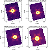 |
Fig. A.1. MRS continuum maps of Mrk 231 in ch1, ch2, ch3, and ch4 at the wavelengths specified at the top of each subpanel. The images are shown in a linear scale (arbitrary units) with cuts chosen to emphasize the low level structure of the point source The star symbol marks the peak of the continuum. The 0,0 point on the axes of each map refers to the center of the corresponding sub-channel array, after rotation. |
Appendix B: Spitzer/IRS spectra
We retrieved Spitzer/IRS fully reduced spectra of Mrk 231 from the Combined Atlas of Sources with Spitzer IRS Spectra (CASSIS, Lebouteiller et al. 2011, 2015). There are several observations taken in different cycles for this galaxy. Figure B.1 shows those from program ID: 1459 (P.I.: L. Armus) using the low-resolution modules (top panel): short-low (SL) with a slit width of 3.6–3.7′′ and long-low (LL) with a slit width of 10.5-10.7′′, and the high-resolution modules (bottom panel): short-high (SH) with a slit width of 4.7′′ and long-high (LH) with a slit width of 11.1′′. CASSIS identified this source as point-like and used the optimal extraction option.
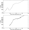 |
Fig. B.1. Spitzer/IRS spectra of Mrk 231. Those obtained with the low-resolution modules SL and LL are in the top panel and those of the high-resolution modules SH and LH in the bottom. Wavelength and flux density ranges are as in Fig. 2. |
Appendix C: Emission line maps
In this appendix, Figs. C.1, C.2 and C.3 present maps of the line intensity, mean-velocity field, and velocity dispersion for the low-excitation lines [Fe II], [Ne III], and [S III], while Figs. C.4 and C.5 for H2 S(2) and H2 S(1) observed in ch4.
Since the [Ne III] and [S III] emission lines show a relatively low contrast with respect to the local continuum, especially in the nuclear region (see Figs. 2 and 3), we smoothed the data cube spaxels along the spatial directions with a 2 × 2 average box before fitting Gaussians to the lines and constructing the maps. Despite this, there are still artificial holes of line emission in the central few spaxels due to the strong continuum. Nevertheless, both line flux maps reveal emission similar to that of [Ne II] (see Fig. 6).
To help identify the SF regions discussed in the text, we marked them in the contour plot of the [Ne II] emission of Fig. C.6. In this case, this intensity map was constructed by integrating the line and subtracting the local adjacent continuum from both sides of the line, instead of fitting a single Gaussian.
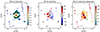 |
Fig. C.1. MRS maps of [Fe II] at λrest = 5.34 μm. We smoothed this sub-channel data cube with a 2 × 2 pixel box in the spatial directions prior to fitting the emission line on a spaxel-by-spaxel basis. Panels and symbol are as in Fig. 5. The 0,0 point on the axes refers to the center of this sub-channel array, after rotation. In all maps, north is up and east to the left. |
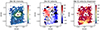 |
Fig. C.2. MRS maps of [Ne III] at λrest = 15.56 μm. We smoothed this sub-channel data cube with a 2 × 2 pixel box in the spatial directions prior to fitting the emission line on a spaxel-by-spaxel basis. Panels and symbol are as in Fig. 5. The 0,0 point on the axes refers to the center of this sub-channel array, after rotation. In all maps, north is up and east to the left. |
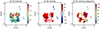 |
Fig. C.3. MRS maps of [S III] at λrest = 18.71 μm. We smoothed sub-channel data cube with a 2 × 2 pixel box in the spatial directions prior to fitting the emission line on a spaxel-by-spaxel basis. Panels and symbol are as in Fig. 5. The 0,0 point on the axes refers to the center of this sub-channel array, after rotation. In all maps, north is up and east to the left. |
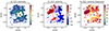 |
Fig. C.4. MRS maps of H2 S(2) line at λrest = 12.28 μm. Panels and symbol are as in Fig. 5. The 0,0 point on the axes refers to the center of this sub-channel array, after rotation. In all maps, north is up and east to the left. |
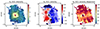 |
Fig. C.5. MRS maps of H2 S(1) at λrest = 17.03 μm observed in ch4. Panels and symbol are as in Fig. 5. The 0,0 point on the axes refers to the center of this sub-channel array, after rotation. In all maps, north is up and east to the left. |
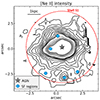 |
Fig. C.6. Contour map of the MRS [Ne II] emission. We mark some of the SF regions discussed in the text. We generated this [Ne II] map by integrating all the line emission and subtracting a local continuum measured on both sides of the line. The black contours are shown in a square root scale, while the gray ones are in a linear scale. |
Appendix D: [Ne II] velocity channel maps
In this appendix, we show in Fig. D.1] the velocity (relative to the systemic value) channel maps for the [Ne II]. We generated them from an extracted data cube around the line after subtracting the local continuum on a spaxel-by-spaxel basis. For each velocity range, the channel maps are plotted for pixels with fluxes three times the standard deviation above the mean value measured in regions with no line emission. The exception is for the channels including the systemic velocity, where there is line emission practically all over the ch3 FoV and the fluxes are those above the mean value in a small region with no line emission.
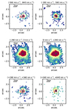 |
Fig. D.1. Velocity (relative to the systemic value) channel maps for [Ne II]. Fluxes are plotted in a square root scale, which is the same in all panels. |
Appendix E: Non-parametric emission line analysis
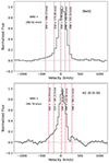 |
Fig. E.1. Non-parametric analysis of two nuclear line profiles: [Ne II] (top panel) and H2 S(5) (bottom panel). The derived velocities (see text for details) are marked with red vertical lines. The gray lines indicate the limits of the emission line defined as fluxes above two times the standard deviation of the (zero) continuum. |
In this appendix, we describe the method followed to perform the non-parametric analysis of the most prominent nuclear emission lines in the nuclear region of Mrk 231.
A non-parametric analysis allows to obtain the kinematic properties of the emission lines without assuming any prior conditions for the line profile, as is the case with a parametric modeling (i.e., Gaussian profiles). This method is exclusively based on measuring the flux of the lines. We used a modified version of the method put forward by Harrison et al. (2014). Instead of using fitted Gaussians to isolate the line, we defined the line with respect to the noise of the zero level continuum. To perform the analysis, we selected a region ranging from −1200 to 1200 km s−1 from the redshifted-corrected central wavelength of the line, and normalised the whole range to the maximum flux (that is, the line peak) after the continuum subtraction. Then we estimated the standard deviation in the continuum near the emission line, and defined the line as all those spectral elements where the flux is larger than two times that value. Then we summed up all the flux of the line within that range and estimated the velocities. The derived velocities are more conservative as this method takes into account the continuum variations, which can include real structure (e.g., broad features) as well as noise. This is especially relevant for lines which do not present a strong contrast against the continuum.
As mentioned in Sect. 7.1, we measured the following parameters v02, v10, v50, v90, and v98, which are the velocities at which we found 2%, 10%, 50%, 90%, and 98% of the line fluxes, and W80, which is a measurement of the line width, defined as abs(v90 − v10). The line width W80 is equivalent to 1.088×FWHM for a single Gaussian-like profile (Harrison et al. 2014). We note that the W80 parameter is not corrected from the instrumental broadening. We also note that the analysis was done on the spectra before the 1D residual fringe correction to avoid removing real spectral features.
As an illustration, Fig. E.1 presents the analysis for [Ne II] and H2 S(5). The uncertainties of the measured velocities only associated with the spectral step of the different sub-channels are of the order of 43 km s−1 for [Fe II], 33 km s−1 for [Ar II] and H2 S(5), 47 km s−1 for H2 S(4), and 56 km s−1 for [Ne II].
All Tables
All Figures
|
Fig. 1. Archival HST/ACS image (color and contours, shown in a square root scale) of Mrk 231. The observation was taken with the optical F435W filter and it shows the central 16″ × 16″, which corresponds to a region of ≃13.4 kpc × 13.4 kpc in size. For reference, the overlaid dashed square represents the approximate FoV and orientation of the MRS ch3 observations. We mark the positions of several expanding shells identified by Lípari et al. (2005) and discussed in the text. |
| In the text | |
|
Fig. 2. MRS nuclear spectrum (solid black line) of Mrk 231. It was extracted with a 1″-radius aperture and covers the rest-frame ∼4.7 − 23.5 μm spectral range. We applied the residual fringing correction to the extracted 1D spectra of each of the sub-channels. The dotted line is the fitted continuum using a cubic spline function and the red dots are the anchor points selected for the fit. |
| In the text | |
|
Fig. 3. Nuclear spectrum shown for each of the MRS channels. As in Fig. 2, the extraction aperture had a 1″-radius. Each panel shows the A, B, and C sub-channels (ch1 upper left, ch2 upper right, ch3 lower left, and ch4 lower right), except for ch4 for which we only show A and B (see text). The dashed lines mark the detected low-excitation fine-structure emission lines (blue and green) and rotational H2 lines (orange). The loosely dotted lines are other relatively low IP lines not detected in the nuclear spectrum (see text for more details). Also labeled are the positions of PAHs, silicate features, and some molecular absorption bands. |
| In the text | |
|
Fig. 4. Zoomed-in spectral regions of the nuclear spectra around the wavelengths of high-excitation lines [Mg V] (top) and [Ne V] (bottom). The black lines are the observed spectra extracted with an aperture radius of 0.5″ (top) and an aperture radius of 1″ (bottom), while the dotted and dashed lines are the predicted high-excitation emission lines from MRS observations of two local AGN assuming an intrinsic 2 − 10 keV luminosity of 1044 erg s−1 for Mrk 231 (see text for details). The ch3-medium spectrum was corrected for residual fringing that was affecting mostly data at wavelengths longer than that of [Ne V]. |
| In the text | |
|
Fig. 5. Maps of [Ar II] at λrest = 6.99 μm. The maps were constructed by fitting a single Gaussian function and a local continuum to the emission line on a spaxel-by-spaxel basis. The panels show the intensity and contours in units of |
| In the text | |
|
Fig. 6. Maps of [Ne II] at λrest = 12.81 μm. Panels and symbol are as in Fig. 5. The 0,0 point on the axes refers to the center of this sub-channel array, after rotation. In all maps, north is up and east to the left. |
| In the text | |
|
Fig. 7. Maps of the intensity of the 11.3 μm PAH feature (top) in units of 10−16 erg cm−2 s−1 and the 11.3 μm PAH to [Ne II] line ratio (bottom). The FoV and symbols are as in Fig. 6. The maps and contours are in a linear scale. |
| In the text | |
|
Fig. 8. Maps of H2 S(5) at λrest = 6.91 μm. Panels and symbol are as in Fig. 5. The 0,0 point on the axes refers to the center of this sub-channel array, after rotation. In all maps, north is up and east to the left. |
| In the text | |
|
Fig. 9. Maps of H2 S(1) at λrest = 17.03 μm observed in ch3. Panels and symbol are as in Fig. 5. The 0,0 point on the axes refers to the center of this sub-channel array, after rotation. In all maps, north is up and east to the left. |
| In the text | |
|
Fig. 10. H2 rotational diagrams for the nuclear region of Mrk 231. The fit was performed with a two-temperature model and assuming LTE conditions (see text for details). Top: using observed values and bottom: using the S(3), S(2), and S(1) fluxes corrected for extinction (see text for details). |
| In the text | |
|
Fig. 11. MRS spectra of the star-forming region 1.1″ SE of the AGN. Top panel: ch1 to ch3 spectra extracted with a 0.3″ radius. We applied the residual fringing correction to the 1D spectra and scaling factors to stitch together the spectra of the different sub-channels. Middle and bottom panels: zoomed-in spectral regions of selected emission lines. In all panels, the rest-frame wavelengths were computed with the redshift quoted in Sect. 1 and appear redshifted with respect to the systemic velocity (see mean-velocity maps of [Ar II] and [Ne II], middle panels of Figs. 5 and 6), due to rotation. |
| In the text | |
|
Fig. 12. Line profiles from the nuclear region (r = 1″ aperture). Left panel: fine-structure lines, and middle and right panels: H2 S(7) to S(4) and S(3) to S(1) transitions, respectively. The 0 km s−1 value corresponds to the adopted z = 0.004217. Note that the red part of the H2 S(6) line profile (green line, middle panel) is inside one of the H2O molecular absorptions. We did not apply the 1D residual fringe correction. |
| In the text | |
|
Fig. 13. Kinematic minor axis p–v diagrams for [Ar II] (left) and [Ne II] (right). The extraction aperture is 2′′. The 0,0 point in the spatial direction marks the AGN position. The first contour is drawn at three times the standard deviation of the (zero) continuum level. The position of the main expanding shells (Lípari et al. 2005) are marked as horizontal lines. In the right panel the vertical lines denote the estimated virial range. |
| In the text | |
|
Fig. 14. Kinematic minor axis p–v diagrams for H2 S(5) (left) and H2 S(1) (right) emission lines. Lines and symbols as Fig. 13. |
| In the text | |
|
Fig. 15. Cartoon summarizing the different regions (not drawn to scale) of Mrk 231 identified with the MRS observations and other literature results. Left: front view, that is, in the plane of the sky, where the molecular gas disk is seen close to face-on. Right: side view to emphasize the possible scenario to explain some of the observed non-circular motions in the ionized and warm molecular gas. |
| In the text | |
|
Fig. A.1. MRS continuum maps of Mrk 231 in ch1, ch2, ch3, and ch4 at the wavelengths specified at the top of each subpanel. The images are shown in a linear scale (arbitrary units) with cuts chosen to emphasize the low level structure of the point source The star symbol marks the peak of the continuum. The 0,0 point on the axes of each map refers to the center of the corresponding sub-channel array, after rotation. |
| In the text | |
|
Fig. B.1. Spitzer/IRS spectra of Mrk 231. Those obtained with the low-resolution modules SL and LL are in the top panel and those of the high-resolution modules SH and LH in the bottom. Wavelength and flux density ranges are as in Fig. 2. |
| In the text | |
|
Fig. C.1. MRS maps of [Fe II] at λrest = 5.34 μm. We smoothed this sub-channel data cube with a 2 × 2 pixel box in the spatial directions prior to fitting the emission line on a spaxel-by-spaxel basis. Panels and symbol are as in Fig. 5. The 0,0 point on the axes refers to the center of this sub-channel array, after rotation. In all maps, north is up and east to the left. |
| In the text | |
|
Fig. C.2. MRS maps of [Ne III] at λrest = 15.56 μm. We smoothed this sub-channel data cube with a 2 × 2 pixel box in the spatial directions prior to fitting the emission line on a spaxel-by-spaxel basis. Panels and symbol are as in Fig. 5. The 0,0 point on the axes refers to the center of this sub-channel array, after rotation. In all maps, north is up and east to the left. |
| In the text | |
|
Fig. C.3. MRS maps of [S III] at λrest = 18.71 μm. We smoothed sub-channel data cube with a 2 × 2 pixel box in the spatial directions prior to fitting the emission line on a spaxel-by-spaxel basis. Panels and symbol are as in Fig. 5. The 0,0 point on the axes refers to the center of this sub-channel array, after rotation. In all maps, north is up and east to the left. |
| In the text | |
|
Fig. C.4. MRS maps of H2 S(2) line at λrest = 12.28 μm. Panels and symbol are as in Fig. 5. The 0,0 point on the axes refers to the center of this sub-channel array, after rotation. In all maps, north is up and east to the left. |
| In the text | |
|
Fig. C.5. MRS maps of H2 S(1) at λrest = 17.03 μm observed in ch4. Panels and symbol are as in Fig. 5. The 0,0 point on the axes refers to the center of this sub-channel array, after rotation. In all maps, north is up and east to the left. |
| In the text | |
|
Fig. C.6. Contour map of the MRS [Ne II] emission. We mark some of the SF regions discussed in the text. We generated this [Ne II] map by integrating all the line emission and subtracting a local continuum measured on both sides of the line. The black contours are shown in a square root scale, while the gray ones are in a linear scale. |
| In the text | |
|
Fig. D.1. Velocity (relative to the systemic value) channel maps for [Ne II]. Fluxes are plotted in a square root scale, which is the same in all panels. |
| In the text | |
|
Fig. E.1. Non-parametric analysis of two nuclear line profiles: [Ne II] (top panel) and H2 S(5) (bottom panel). The derived velocities (see text for details) are marked with red vertical lines. The gray lines indicate the limits of the emission line defined as fluxes above two times the standard deviation of the (zero) continuum. |
| In the text | |
Current usage metrics show cumulative count of Article Views (full-text article views including HTML views, PDF and ePub downloads, according to the available data) and Abstracts Views on Vision4Press platform.
Data correspond to usage on the plateform after 2015. The current usage metrics is available 48-96 hours after online publication and is updated daily on week days.
Initial download of the metrics may take a while.