| Issue |
A&A
Volume 693, January 2025
|
|
|---|---|---|
| Article Number | A106 | |
| Number of page(s) | 15 | |
| Section | Extragalactic astronomy | |
| DOI | https://doi.org/10.1051/0004-6361/202451679 | |
| Published online | 07 January 2025 | |
The effect of dynamical states on galaxy cluster populations
I. Classification of dynamical states
1
Departamento de Astronomía, Universidad de La Serena, Av. Raúl Bitrán 1305, La Serena, Chile
2
International Gemini Observatory, NSF’s NOIRLab, Casilla 603, La Serena, Chile
3
Cerro Tololo Inter-American Observatory, NSF’s NOIRLab, Casilla 603, La Serena, Chile
⋆ Corresponding author; This email address is being protected from spambots. You need JavaScript enabled to view it.
Received:
27
July
2024
Accepted:
22
November
2024
Abstract
Context. Although the influence of galaxy clusters on galaxy evolution is relatively well understood, the impact of the dynamical states of these clusters is less clear. This series of papers explores how the dynamical state of galaxy clusters affects their galaxy populations’ physical and morphological properties.
Aims. The primary aim of this first paper is to evaluate the dynamical state of 87 massive (M500 ≥ 1.5 × 10¹⁴ M⊙) galaxy clusters at low redshifts (0.10 ≤ z ≤ 0.35). This allowed us to obtain a well-characterized sample for analyzing the relevant physical and morphological properties, planned for our next work.
Methods. We employed six dynamical state proxies that utilize optical and X-ray imaging data. We applied a principal component analysis to integrate these proxies effectively, allowing for a robust classification of galaxy clusters into relaxed, intermediate, and disturbed states based on their dynamical characteristics.
Results. The methodology successfully segregates the clusters of galaxies into the three dynamical states. An examination of the projected galaxy distributions in optical wavelengths and gas distributions in X-ray further confirms the consistency of these classifications. The dynamical states of the clusters are statistically distinguishable, providing a clear categorization for further analysis.
Key words: galaxies: clusters: general
© The Authors 2025
 Open Access article, published by EDP Sciences, under the terms of the Creative Commons Attribution License (https://creativecommons.org/licenses/by/4.0), which permits unrestricted use, distribution, and reproduction in any medium, provided the original work is properly cited.
This article is published in open access under the Subscribe to Open model. This email address is being protected from spambots. You need JavaScript enabled to view it. to support open access publication.
1. Introduction
In the context of the standard Lambda cold dark matter (ΛCDM) cosmological model, small fluctuations in the initial density field are amplified by gravity, collapsing into dark matter halos and transitioning from a linear to a nonlinear regime (Molnar 2016). Following the hierarchical paradigm of structure formation, mergers with similarly sized systems and smooth accretions of smaller structures lead to the formation of galaxy clusters (Kravtsov & Borgani 2012), which are the largest gravitationally bound systems in the Universe.
Due to their formation processes, galaxy clusters can exist in various dynamical states. These range from systems close to virialization to highly perturbed systems resulting from large-scale interactions. According to the ΛCDM cosmological model and observations, around 30–80% of the clusters are in unrelaxed states, exhibiting notable substructures in optical and X-ray images (e.g., Dressler & Shectman 1988; Santos et al. 2008; Fakhouri et al. 2010) and merger features in radio images (e.g., Skillman et al. 2013; Golovich et al. 2019)
Galaxy clusters in a relaxed dynamical state are crucial for studying various astrophysical aspects. For instance, they allow us to investigate the advanced stages of structure evolution in the Universe, providing insight into how galaxy clusters have evolved from their initial states to their current form (e.g., Voit 2005). Additionally, due to their higher degrees of symmetry, these systems are ideal for studying dark matter density profiles through gravitational lensing (e.g., Umetsu et al. 2014). Furthermore, since the hot gas forming the intracluster medium (ICM) tends to be in hydrostatic equilibrium in relaxed clusters, more precise studies of its temperature and density distribution can be conducted, offering valuable information about the physics of gas and its cooling history (e.g., Vikhlinin et al. 2006). Moreover, considering that relaxed clusters exhibiting strong gravitational lensing are more numerous than their disturbed counterparts, they are ideal systems for studying high-redshift galaxies that are magnified by this effect. (e.g., Bayliss et al. 2011; Bouwens et al. 2014).
On the other hand, unrelaxed clusters offer different aspects of the study. These systems provide insights into the processes of large-scale structure formation in the Universe, such as merger dynamics or shock waves and cold fronts (e.g., Markevitch et al. 2002; Poole et al. 2006; Owers et al. 2014). Additionally, interactions within galaxy clusters can displace dark matter and ICM components, offering an ideal scenario for studying both components and their interactions (e.g., Clowe et al. 2006; Jee et al. 2014). Moreover, galaxy cluster merger scenarios can be helpful in the field of particle physics to constrain the cross section of self-interacting dark matter particles (e.g., Harvey et al. 2015) and in cosmology, providing essential tests for the standard ΛCDM cosmological model (e.g., Thompson et al. 2015).
Various proxies have been used to classify systems according to their dynamical states. For example, in the projected sky plane, the cluster morphology in radio images has been utilized (e.g., Cassano et al. 2010), as well as the galaxy density distribution (e.g., Wen & Han 2015), surface-brightness distribution in X-rays (e.g., Jeltema et al. 2005; Nurgaliev et al. 2013), and offset between the brightest cluster galaxy (BCG) and the X-ray peak and centroid (e.g., Mann & Ebeling 2012; Zenteno et al. 2020). In addition, to identify cluster mergers along the line of sight, the shape of the velocity distribution has also been used as a proxy (e.g., Ribeiro et al. 2013; de Los Rios et al. 2016; Carrasco et al. 2021).
However, one of the most fundamental aspects of galaxy clusters is that they serve as ideal laboratories for studying galaxy evolution. These are the highest density environments in the Universe’s large-scale structure, where specific physical processes accelerate galaxy evolution, leading to morphological transformations, environmental quenching, and preferential galaxy distributions. Although differences in physical and morphological properties between clusters and the field or other low-density environments have been well studied, the effect of the dynamical state of galaxy clusters on their member galaxies is not entirely clear. Ribeiro et al. (2013) found that the faint end of the luminosity function is more pronounced in relaxed clusters than in disturbed systems at low redshift (z ≤ 0.1) in clusters with M > 1014 M⊙. However, Zenteno et al. (2020) found results that displayed a considerable disagreement. By studying a sample of 288 massive galaxy clusters (M200 > 4 × 10¹⁴ M⊙) with multiwavelength information, they found that the luminosity function does not show statistically significant differences between relaxed and disturbed clusters at low redshift (z ≲ 0.55). However, at a higher redshifts (z ≳ 0.55), disturbed clusters exhibit a more pronounced faint end slope than their relaxed counterparts. It was hypothesized that galaxy cluster populations show differences between relaxed and disturbed clusters at z ≳ 0.55. This corroborated by Aldás et al. (2023), at least in the color-magnitude relation of these systems.
In this series of two papers, we aim to investigate the impact of the dynamical state of massive clusters (M500 ≥ 1.5 × 10¹⁴ M⊙) on the physical and morphological properties of their member galaxies, in the redshift range of 0.10 < z < 0.35. In this first paper, our aim is to detail the sample selection and use optical data from the DESI Legacy Imaging Survey Data Release 10 and X-ray data from the Chandra and XMM-Newton archives to determine the dynamical state of the clusters. The calculation of the physical and morphological properties of the galaxies, as well as the analysis of the impact of the dynamical state on these galaxy populations, will be presented in a second article (Véliz Astudillo et al., in prep., hereafter Paper II).
This paper is organized as follows. Section 2 describes the data and the sample selection process. In Section 3, we detail the method used to assign cluster memberships, followed by the approach used to select the BCGs in Section 4. We define the dynamical state proxies in Section 5. In Section 6, we classify the dynamical state of galaxy clusters, explaining the chosen method. We discuss the results and present the conclusions in Section 7.
Throughout this work, we adopt a flat ΛCDM cosmology, assuming H0 = 69.3 km s−1, ΩΛ = 0.721 and Ωm = 0.287 (WMAP-9, Hinshaw et al. 2013). Unless specifically stated, the magnitudes used in this article are given in the AB system.
2. Data
2.1. DESI Legacy Survey Data Release 10
The DESI Legacy Imaging Survey (Legacy Survey, LS) is the result of the efforts of three different surveys that provide images and catalogs, initially planned for the g, r, and z filters. On the one hand, there are surveys in the northern hemisphere (δ ≳ 32); these include the Beijing Arizona Sky Survey (BASS, Zou et al. 2017), which provides photometric information in the g and r bands using the Bok 2.3 m Telescope, and the Mayall z-band Legacy Survey (MzLS, Silva et al. 2016). On the other hand, for the southern hemisphere, there is the Dark Energy Camera Legacy Survey (DECaLS, Blum et al. 2016), which makes use of the Dark Energy Camera (DECam) mounted on the Victor Blanco 4 m Telescope in the g, r, and z filters. It is worth mentioning that DECaLS is primarily composed of data from the Dark Energy Survey (DES, The Dark Energy Survey Collaboration 2005), with the remaining data obtained from the public DECam data, available in the NOIRLab online repository. Among these earlier programs, the DECam Local Volume Exploration Survey (DELVE, Drlica-Wagner et al. 2022), and the DECam eROSITA Survey (DeROSITAS; PI: Zenteno). The initial goal of LS was to select targets for the upcoming DESI Spectroscopic Survey, whose spectrograph will be installed on the 4 m Mayall Telescope, precisely where the MzLS is conducted.
The latest data release (LS DR10) includes DECam i band data. Altogether, the images from LS DR10 cover more than 20 000 square degrees of the sky, with the three surveys having similar observational design properties. In each filter, a uniform depth of 5σ is reached at mg = 24.7, mr = 23.9, mz = 23.0, which is typically ∼1 magnitude deeper than Pan-STARRS (Duncan 2022). Detailed descriptions of source detection and photometry can be found in Dey et al. (2019, and references therein).
On the official LS DR10 website1, the project’s catalogs and images are available. With respect to the catalogs, they were generated using the software THE TRACTOR (Lang et al. 2016). This code employs a probabilistic method to fit surface brightness models to the sources in an image. The models can be point sources (PSF), round exponential galaxies with variable radius (REX), de Vaucouleurs (DEV) profiles (elliptical galaxies), exponential (EXP) profiles (spiral galaxies), and Sersic (SER) profiles, and these are fitted employing a χ2 minimization problem. It is worth noting that in addition to optical data, the catalogs also include infrared information from the Wide-field Infrared Survey Explorer (WISE) five-year coadded image, also known as unWISE (Wright et al. 2010), in the W1, W2, W3, and W4 bands. Concerning the images, we utilized science images, weight images, exposure number maps, and full-width half-maximum maps.
2.2. Chandra and XMM-Newton archive images
The X-ray images used in this study were obtained from the Chandra and XMM-Newton archives. However, it is important to note that the entire process, from the downloading of the images to their uniform processing and availability in repositories, was carried out by other authors and is accessible to the scientific community. Specifically, Yuan & Han (2020) initiated their project to evaluate the dynamical state of galaxy clusters based on the morphology of the X-ray surface brightness distribution, revealing the behaviors of the ICM in these systems. In their study, they explain that the Chandra satellite has observed approximately ∼1000 galaxy clusters, and the high resolution of its images is ideal for detecting substructures in the ICM. They processed the data from these structures by filtering photons with energies in the 0.5–5.0 keV range, carefully removing flares and point sources, and smoothing the images with a Gaussian kernel at a physical scale of 30 kpc. Initially, these scales varied for each cluster due to their different redshifts.
Subsequently, Yuan et al. (2022) expanded on their previous work, this time including data from ∼1300 XMM-Newton systems and 22 new Chandra-observed clusters in the period between their two studies. The processing of X-ray images was the same for consistency, resulting in a total of 1844 galaxy clusters between the two studies. In addition, parameters were calculated for all these clusters to approximate their dynamical states (detailed in Section 5). Thus, the final data products, consisting of images and catalogs, are publicly available on the authors’ web repository2.
2.3. Redshift catalogs
This study uses the photometric redshift catalog from Wen & Han (2022). Using data from DES and unWISE, they estimated the photometric redshifts of 105 million galaxies, employing clustering algorithms to identify 151 244 galaxy clusters in the redshift range of 0.1 < z < 1.5. The algorithms used are explained in detail in Wen & Han (2021). In summary, the authors used publicly available DES DR2 data in the grizY bands (Abbott et al. 2021) and unWISE data in the W1 and W2 filters. The match between both databases results in 105 million objects. Then, photometric redshifts were derived on the basis of colors using the nearest-neighbors algorithm with respect to the spectroscopic redshifts of a robust training sample. Specifically, the distances from the target galaxies to all training galaxies in the multidimensional color space (g − r, r − i, i − z, z − y, y − W1, and W1 − W2) were calculated. Then, the 20 nearest neighbors were selected to compute the photometric redshift. This was calculated as the mean value of these 20 neighbors with spectroscopic redshift and the error was calculated as the standard deviation among them. This methodology is based on the premise that the color of galaxies is closely related to their redshifts when covering spectral features such as the 4000 Å break or the Balmer jump. Galaxies close to the multidimensional color space generally have similar redshifts (Wen & Han 2021).
We conducted an exhaustive literature search to find galaxy clusters with spectroscopic information in their respective fields. The selection process of these systems is detailed in Section 2.4, and Table 1 shows the sources from which the spectroscopic information was obtained.
Galaxy clusters with spectroscopic redshifts available in the literature.
Figure 1 shows the comparison between the photometric redshifts obtained from the catalogs of Wen & Han (2022) and the spectroscopic redshifts obtained in the literature for the member galaxies of the clusters. We defined Δznorm = (zphot − zspec)/(1 + zspec) and found a mean value of Δznorm = 0.005 with a dispersion of σz = 0.02, using robust biweight estimators.
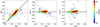 |
Fig. 1. Comparison of spectroscopic and photometric redshifts (zspec and zphot) and the normalized redshift deviation (Δznorm). Left: Comparison between zspec and zphot. The solid black line represents the identity line (zspec = zphot). Middle: Δznorm as function of zspec. Right: Δznorm as function of zspec. In the latter two cases, the solid black line corresponds to the constant function where Δznorm = 0. |
2.4. Sample selection
If we want to study the effect of cluster dynamics on the morphology of their member galaxies, having a robust and homogeneous sample is crucial. To achieve this, we performed a 2 arcminute radius cross-match between the galaxy clusters identified in the optical by Wen & Han (2022) and those in X-rays found in the Chandra (Yuan & Han 2020) and XMM-Newton (Yuan et al. 2022) archives, resulting in 471 systems.
Then, we selected those galaxy clusters in the redshift range of 0.10 < z < 0.35, resulting in 152 clusters. At this point, Abell 3827 is added, at z ∼ 0.099, and we have access to spectroscopic information. The lower limit is chosen mainly because of the extensive spatial coverage required for nearby clusters. Regarding the upper limit, we rely on the work of de Albernaz Ferreira & Ferrari (2018), demonstrating that reliable morphological studies can be performed using DECam up to z ∼ 0.4. However, we decided to be conservative and study up to the mentioned limit. Furthermore, within this interval, it ensures that we cover the 4000 Å break using the (g − r) color index to separate early-type red galaxies from star-forming objects (e.g., Bruzual 1983; Nilo Castellón et al. 2014). Moreover, within this redshift range, the LS DR10 achieves enough photometric depth to conduct homogeneous studies up to three magnitudes fainter than the characteristic magnitude (m* + 3) of all clusters in the sample.
Subsequently, to ensure that the matching of clusters between optical and X-ray databases would not be affected by projection effects, we imposed the condition that zx − zphot/(1 + zx)≤0.05. Here, zx is the redshift found in the X-ray catalogs of Yuan & Han (2020) and Yuan et al. (2022), while zphot is the photometric redshift estimated for the clusters identified in the optical wavelengths by Wen & Han (2022), resulting in 119 galaxy clusters. Next, we removed all systems that are very poor and low-mass from the sample by applying the condition λ ≥ 30 and M500 ≥ 1.5 × 10¹⁴ M⊙, where λ is the cluster richness estimated based on overdensities and fluctuations in the field and M500 is the mass of the clusters estimated within R500, with calculations detailed in Wen & Han (2022). Finally, the last filter was applied to exclude, via a visual inspection, all systems with field contamination due to a saturated star or lack of photometric information in the LS catalogs. Our final sample consists of 87 massive galaxy clusters.
3. Cluster membership
The most unequivocal way to select member galaxies of a cluster is by using spectroscopic redshifts. However, for our sample, less than half of the clusters have catalogs of this nature available in the literature or databases such as NED3 or Vizier4. Additionally, there is the difficulty of the few systems with this information not sharing the same observational designs. For example, some systems have more than 1000 galaxies with spectroscopic data in the field due to the use of integral field spectroscopy (e.g., Mercurio et al. 2021) or multiobject spectroscopy (e.g., Owers et al. 2011). In contrast, others have fewer than 20 objects due to the use of a few slits, mainly selecting galaxies that are on the red sequences (RS) in the color-magnitude diagrams (CMDs) of the clusters (e.g., Bayliss et al. 2016). Additionally, there are differences in sky coverage and/or limit magnitudes. These differences can directly affect sample analyses, leading to biased results due to inhomogeneities. However, this can be addressed by homogeneously assigning membership to the entire sample using only photometric redshifts.
In this way, we have followed a probabilistic method, the foundations of which were established by Brunner & Lubin (2000) and later developed by Pelló et al. (2009). The procedure consists of calculating the probability, Pmember, of a galaxy’s membership to a cluster at redshift, zcl, within a redshift slice, δz, as
 (1)
(1)
To define the redshift slice, we followed Kesebonye et al. (2023), using δz = nσbw(1 + zcl), with n = 2. To determine σbw, we used all galaxies with available spectroscopic redshifts (see Table 1) to compare them with photometric redshifts, obtaining a mean residual of (zspec − zphot)/(1 + zspec) = 0.008. The robust biweight scale estimator (Beers et al. 1990) resulted in σbw = 0.02.
Here, P(z) is the galaxy photometric redshift probability distribution, discussed in the literature. We note that it does not have to be Gaussian; instead, it can have multiple peaks or extended tails (Pelló et al. 2009). For this reason, the photometric redshift distributions provided as output in codes that calculate this value have been used in other works (e.g., De Lucia et al. 2004; Vulcani et al. 2012; Kesebonye et al. 2023). These distributions are usually obtained using algorithms that involve fitting SEDs to a library of templates. However, we do not have this information; we only have the photometric redshift information and its corresponding error. Thus, we approximated this distribution as a Gaussian with μ = zphot and σ = zphot, err. Although we recognize the mentioned disadvantages, at least we were able to consider the measurement error and it is feasible to apply this probabilistic method instead of making a simple selection within a photometric redshift slice.
The method requires a calibration of Pmember with spectroscopic data; in turn, this allows for the calculation of the completeness of cluster member galaxies and contamination by field galaxies. We performed this calibration using clusters that have spectroscopic redshifts for a large number of both member and field galaxies, specifically Abell 267, Abell 383, Abell 2537, Abell 2631, Abell 2744, Abell S1063, and RBS 1748. We selected spectroscopically confirmed member galaxies using |zcl − zspec|< 3σcl(1 + zcl), where σcl is the velocity dispersion of the cluster.
We identified 1041 member galaxies and 1328 galaxies that do not belong to the mentioned clusters. In Fig. 2, the completeness and contamination fractions can be observed for a range of Pthreshold values. We explored 100 variations for this parameter, from 0 to 1, in steps of 0.01. With this calibration, we decided to use the value of Pthreshold = 0.65, ensuring a completeness of at least 80% and contamination below 25%5. This photometric redshift quality, completeness, and contamination levels work well for our purposes, as we plan to study the integrated properties of cluster galaxy populations, rather than the individual properties of galaxies. Moreover, as we explain in Section 5, we used X-ray data and the position of the BCG derived from optical images to evaluate the dynamical state of galaxy clusters and we do not aim to find substructures using member galaxies selected with photometric redshifts. In addition, we applied a magnitude limit to the study sample. We used a criterion of m < m* + 3 in the r band. This ensures a homogeneous selection of members for all clusters across the whole redshift range.
 |
Fig. 2. Fraction of retained members (completeness, black dots) and non-members (contamination, gray crosses) as a function of the probability threshold Pthreshold. This figure was created using only galaxies with secure zspec measurements in clusters with enough spectroscopic data for members and the field. |
In Fig. 3 we show the spatial coverage of the selected members in R200. We split the clustercentric distance into ten symmetrical bins, and we present the median values along with the first and third quartiles, as a measure of dispersion. It can be seen that the variations are very small (the maximum dispersion is lower than 3%). This means that the clusters do not present any bias in the spatial distribution and that they are indeed comparable.
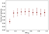 |
Fig. 3. Fraction of galaxies as function of the clustercentric distance for the stacked sample of galaxy clusters. Dark red points correspond to the median values in each bin, while the lower and upper error bars are the first and third quartile in each bin, respectively. |
4. Brightest cluster galaxy selection
Identifying the BCG is crucial for estimating the dynamical state of galaxy clusters. We selected the BCG using a combination of an automatic method and visual inspection.
The automatic method involves selecting the brightest cluster member galaxy within ±1σ of the best fit to the red cluster sequence in the normalized color-magnitude diagram of each galaxy cluster. Several studies have shown that the evolution of the characteristic magnitude, m*, for galaxy cluster populations can be described by a stellar population formed at high redshift that evolves passively (e.g., de Propris et al. 1999; Andreon 2006; Stalder et al. 2013). This has been reproduced over a broad redshift range (0 ≲ z ≲ 1) for massive clusters (Zenteno et al. 2016, 2020). To model m*, we created red sequence composite stellar populations (CSP) for the DECam griz bands using Bruzual & Charlot (2003) SSP models via the Python code EZGAL (Mancone & Gonzalez 2012). Specifically, we assumed an exponentially declining star formation rate with a characteristic decay time of 0.4 Gyr, the Chabrier initial mass function (IMF), and a single burst of star formation at z = 3 followed by passive evolution to z = 0. Next, we define normalized magnitudes as
 (2)
(2)
where m is the magnitude of each galaxy. This allows us to compare the CMDs of galaxy clusters despite differences in redshift as we consider the cluster redshift and K-corrections6 in the applied models. Note that we inherently define normalized colors that correspond to the subtraction of two normalized magnitudes.
Subsequently, we fit a double Gaussian model to the normalized color distribution (g − r)norm of each galaxy cluster using a magnitude limit of rnorm = 3, namely, r = m* + 3. This is based on the well-known bimodal color distribution in the member galaxies of these systems, featuring both the blue cloud and the red sequence (e.g., Baldry et al. 2004; Balogh et al. 2004; Menci et al. 2005). We defined the red_limit as μred − 3σred, where μred and σred correspond to the mean value and standard deviation of the Gaussian fitted to the red component, respectively. An example of these double Gaussian fittings for a cluster for each dynamical state is shown in Fig. 4.
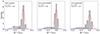 |
Fig. 4. Double Gaussian fits applied to the normalized color distribution of each cluster. From left to right panels, Abell 3827 (relaxed cluster), Abell 3739 (intermediate cluster), and Abell 2744 (disturbed cluster) are presented as examples. The colors of the Gaussians are associated with the red and blue components of the galaxy clusters. The black dashed line indicated the red_limit in each panel. The specific value of this parameter is located in the upper left corner of each panel along with the χ2 statistic for each fit performed with LMFIT. |
Afterward, we select the red galaxies from each galaxy cluster as those where (g − r)norm> red_limit and apply a robust linear regression using the HuberRegressor (Huber & Ronchetti 2011) to fit the red sequence (Fig. 5). This regression model has the advantage of being less influenced by the presence of outliers. To achieve this, the sample is divided into two groups, with inliers having an absolute error smaller than a certain threshold. Those that do not meet this condition are considered outliers and given less weight. Specifically, the HuberRegressor optimizes the squared loss for the sub-sample where |(y − Xw − c)/σ|< ϵ (inliers) and the absolute loss for the sub-sample, where |(y − Xw − c)/σ|> ϵ (outliers), where the model coefficient w, intercept c and scale σ are the parameters to optimize. To achieve a statistical efficiency of 95%, this threshold ϵ was set to 1.35. The brightest galaxies within 1σ of the best RS fit of each cluster are selected as BCG candidates.
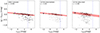 |
Fig. 5. Normalized color-magnitude diagrams for the same clusters mentioned in Fig. 4. Black dots correspond to galaxies selected as members using the probabilistic method with photometric redshifts. Green triangles represent galaxies pre-selected as BCGs using the automated method, while purple inverted triangles denote visually confirmed BCGs. The solid red lines represent the best fits of the red sequences calculated with HuberRegressor and the red shaded areas are the 1σ regions of them. The vertical blue dashed lines indicate the magnitude limit for studying physical and structural properties, namely, m* + 3, where m* is the characteristic magnitude at each cluster redshift modeled with CPS. |
Finally, we visually inspect the BCGs to confirm that the selection was correct. To do this, we followed the approach of Zenteno et al. (2020), considering several properties, including size, colors, number of neighboring galaxies, and their proximity to X-ray peaks.
It is important to note that the method that we ultimately used to discern the BCG of each system is visual inspection, which is particularly useful for measuring the accuracy of the automatic process. However, it is crucial to ensure with spectroscopic information that the galaxy selected as the BCG truly belongs to the cluster. More details on the accuracy of both methods are given in Section 7.1.
5. Proxies of dynamical states
In this subsection, we define the six dynamical state proxies that we utilize. The first two correspond to the offset between the BCG and the X-ray peak and centroid and are calculated directly by us. The next four were calculated by Yuan & Han (2020) and Yuan et al. (2022), and we extracted the values from their catalogs. The reason behind the choice of using six parameters together is that each has its limitations, as we describe below, and their combination can provide us with more robust results.
5.1. BCG-X-ray centroid/peak offset
Considering the highly hydrodynamically collisional nature of the hot gas composing the ICM of galaxy clusters and the typical positioning of the BCG within the deepest region of its gravitational potential well, the BCG can be effectively used as a proxy for the non-collisional dark matter component. Thus, the offset between the position of the X-ray emission peak and centroid and the BCG provides a good approximation of the dynamical state of clusters, at least in the projected sky plane. This is because the components would be noticeably displaced in a merger process between these structures. Following Mann & Ebeling (2012), we used a threshold to distinguish between relaxed and disturbed clusters, with a value of DBCG-X = 42(71) kpc for the X-ray peak (centroid) offset.
5.2. Morphological parameter δ
This parameter is a morphological indicator of the X-ray surface brightness distribution. The definition of Yuan & Han (2020) mentions that the great advantage of this dynamical parameter is its adaptability to the properties of each cluster, allowing for a direct comparison to be made between them. The first step in calculating the value of δ is to fit a 2D elliptical β model to the X-ray surface brightness distribution. Then, a new parameter of the X-ray distribution profile can be calculated as
 (3)
(3)
where β and ϵ are the power-law index and ellipticity of the fitted β-model, respectively.
Based on the observation that disturbed clusters tend to have a more asymmetric geometry than relaxed clusters (e.g., Okabe et al. 2010; Zhang et al. 2010), the asymmetry factor α is used as an auxiliary variable.
![Mathematical equation: $$ \begin{aligned} \alpha = \frac{\sum _{x_i, y_i} [f_{\text{ obs}} (x_i, y_i) - f_{\text{ obs}} (x\prime _{i}, y\prime _{i})]^2}{\sum _{x_i, y_i} f^2_{\text{ obs}} (x_i, y_i)} \times 100 \text{ per} \text{ cent}, \end{aligned} $$](/articles/aa/full_html/2025/01/aa51679-24/aa51679-24-eq4.gif) (4)
(4)
where, fobs(x′i, y′i) is the flux observed in the pixel symmetric to fobs(xi, yi) with respect to the center of the cluster (x0, y0), obtained from the fit of the β-model.
With a combination of these parameters that quantify the properties of the profiles and the asymmetry of the X-ray surface brightness distribution, the morphological index δ is defined as:
 (5)
(5)
To find appropriate values for the free parameters, Yuan & Han (2020) used a homogeneous calibration sample of 125 clusters qualitatively classified by Mann & Ebeling (2012), finding that the values of A = 0.68, B = 0.73, and C = 0.21 can separate the sample into relaxed systems (δ < 0) and disturbed systems (δ ≥ 0), with a success rate of 88%.
5.3. Concentration index: c
Galaxy clusters in a non-virialized state may exhibit various substructures or extended geometries. However, when these systems are very close to virialization, most of the matter is concentrated in their center, with some even having very luminous cool cores (e.g., Fabian et al. 1994; McDonald et al. 2012, 2013). The concentration index, c, quantifies this characteristic by being calculated as the ratio of the integrated X-ray flux within an inner aperture to that within an outer aperture. We followed the definition of Cassano et al. (2010, 2013), which uses apertures of 100 kpc and 500 kpc:
 (6)
(6)
where fobs(xi, yi) is the flux observed in the pixel (xi, yi).
Cassano et al. (2010) found that the median distribution of the concentration parameter log(c) = − 0.7 is a reasonable threshold to distinguish galaxy clusters in different dynamical states. These states were classified based on their features observed in radio images.
5.4. Centroid shift: ω
In relaxed clusters, there is an almost negligible deviation between the positions of the X-ray peak and the X-ray centroid. However, these two positions can exhibit a considerable shift in clusters that undergo mergers. Poole et al. (2006) quantified the deviation between the X-ray peak and the center of a model fit within 20 apertures of different sizes centered on the X-ray peak. The aim was to obtain a value that helps determine the dynamical state of the cluster. This is an iterative process that starts from 0.05 Rap and increases to Rap in increments of 0.05 Rap. In other words,
![Mathematical equation: $$ \begin{aligned} \omega = \left[ \frac{1}{n-1} \sum _i (\Delta _i - \langle \Delta \rangle )^2 \right]^{\frac{1}{2}} \times \frac{1}{R_{\text{ ap}}}\cdot \end{aligned} $$](/articles/aa/full_html/2025/01/aa51679-24/aa51679-24-eq7.gif) (7)
(7)
Here, Rap = 500 kpc, n = 20, Δi is the distance between the peak of the X-ray surface brightness and the center of the fitted model in the i-th aperture, and ⟨Δ⟩ is the mean value of all Δi. Similarly to concentration c, Cassano et al. (2010) found that log(ω) = − 1.92 is a good threshold for separating relaxed and disturbed systems.
5.5. Power ratio P3/P0
Based on the observation that systems undergoing mergers or with substructures exhibit more fluctuations in X-ray surface brightness, Buote & Tsai (1995) derived dimensionless powers from the 2D multipole expansion of the projected gravitational potential of clusters within Rap = 500 kpc.
![Mathematical equation: $$ \begin{aligned} P_0 = [a_0 \ln (R_{\text{ ap}})]^2, \end{aligned} $$](/articles/aa/full_html/2025/01/aa51679-24/aa51679-24-eq8.gif) (8)
(8)
for m = 0, and
 (9)
(9)
for m > 0.
Here, the moments am and bm are given by
 (10)
(10)
 (11)
(11)
where r is the distance to the pixel (xi, yi) from the center of the cluster (x0, y0), and fobs(xi, yi) is the flux observed in that pixel.
It has been empirically found that the power ratio P3/P0 is a good parameter to separate clusters according to their dynamical states. In this work, we use log(P3/P0) = − 6.92 as a threshold, considering clusters with a value lower (higher) than this threshold as relaxed (disturbed) systems. This choice, like the parameters c and ω, is based on the article by Cassano et al. (2010), where the thresholds are defined as the medians of the distributions.
6. Dynamical states of galaxy clusters
As mentioned earlier, dynamical parameters alone do not robustly separate galaxy cluster samples. This is due to various factors appropriately discussed in the articles in which they were developed (i.e., Buote & Tsai 1995; Poole et al. 2006; Cassano et al. 2010; Mann & Ebeling 2012; Yuan & Han 2020). For example, parameters such as c, ω, and P3/P0 are calculated on fixed apertures. However, clusters have different sizes, so the values derived from these apertures may not be entirely comparable. That is why Yuan & Han (2020) decided to develop a new parameter (δ), which is adaptable to the size of these systems. Nonetheless, the parameter alone still has a considerable overlapping region.
If we add the offsets of the BCG with the X-ray peak and centroid to the parameters, as mentioned earlier (which are pretty robust proxies due to their multiwavelength nature and the components they approximate in each structure), then we propose that we can more robustly approximate the dynamical state of galaxy clusters.
A method that might initially seem effective is to create a Boolean sum of disturbance conditions. Then, one could observe the distribution of this Boolean sum and categorize the sample into relaxed and disturbed clusters, perhaps with an intermediate region. However, as seen in Fig. 6, several parameters are correlated with each other, either positively or negatively. Therefore, this method could potentially give more statistical weight to one parameter over another, leading to biased results.
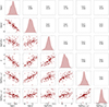 |
Fig. 6. Correlation matrix of the six dynamical state proxies used in this work. The diagonal displays the kernel density estimation (KDE) of each variable. Below the diagonal, scatter plots with linear fits and their corresponding confidence intervals are presented for all combinations of these parameters. Above the diagonal, the Pearson correlation coefficients associated with each parameter space are shown. |
To address this situation, we took advantage of the fact that some clusters in our study sample have dynamical states determined using other methods, such as visual inspection of features in radio and a combination of optical and X-ray observations. We searched for those clusters in the literature, creating a subset that consists of 26 systems with well-defined dynamical states (Table 2), which we used to calibrate our method.
Galaxy clusters with known dynamical states from literature used to calibrate our method.
Subsequently, we applied a principal component analysis (PCA) to this subsample. This is a statistical tool that uses a linear transformation to reduce the dimensionality of a dataset by identifying (linearly) correlated variables and eliminating noise and redundancy in the data. The advantage of this technique is that it can transform a set of possibly related variables into another set of more fundamental independent variables (Hotelling 1933). Additionally, if the redundancy is significant and, hence, there is a correlation between the variables, it might be possible to reproduce the original values of the variables with fewer principal components than the original number of variables in the dataset without losing their features.
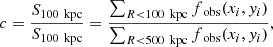
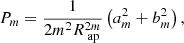
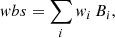
Thus, we applied a PCA to our set of variables {DBCG-XP, DBCG-XP,δ, c, ω, P3/P0}. In Fig. 7, we show that the first principal component (PC 1) can roughly separate the sample into relaxed and disturbed clusters. With this observation, we extract the statistical weights of each dynamical parameter associated with PC 1 (see Table 3). Subsequently, we performed a weighted Boolean sum to determine the dynamical state of the clusters as:
 (12)
(12)
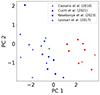 |
Fig. 7. Parameter space of the first two principal components (PC 1 and PC 2) obtained from the six dynamic parameters described in Section 5 for the 26 clusters in the sample that have a well-defined dynamical state in the literature. Blue, red, and green symbols represent relaxed, disturbed, and intermediate clusters, respectively. Crosses, dots, squares and triangles correspond to the data extracted from Cassano et al. (2010), Cuciti et al. (2021), Kesebonye et al. (2023), and Lovisari et al. (2017), respectively. |
Normalized statistical weight of the dynamical parameters associated with the first principal component.
where wi is the statistical weight extracted from PCA and Bi is the Boolean value.
As observed in the distribution of the weighted Boolean sum (wbs) in Fig. 8, it is helpful to divide the sample into three categories: relaxed clusters (wbs < 0), intermediate clusters (0 ≤ wbs ≤ 1), and disturbed clusters (wbs > 1). This is the criterion that we use throughout this work. Furthermore, using the wbs criterion to estimate the dynamical state of galaxy clusters, we identified 32 relaxed clusters, 30 systems in an intermediate dynamical state, and 25 disturbed galaxy clusters.
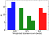 |
Fig. 8. Distribution of the wbs parameter for all the galaxy clusters in the sample. We classify relaxed clusters as systems with wbs < 0 (blue bars), disturbed clusters with wbs > 0 (red bars), and the remaining clusters in between as an intermediate population of galaxy clusters (green bars). |
In Fig. B.1, the scaled values for each proxy are shown, with the dynamical states of each system represented by the colors blue, green, and red for the relaxed, intermediate, and disturbed clusters, respectively. The values of each parameter were scaled using the STANDARDSCALER class from the SCIKIT-LEARN Python package. We note that except for the concentration parameter, the relaxed clusters generally have values lower than the disturbed clusters for the dynamical state proxies, leaving the intermediate clusters with values precisely in between the two. Furthermore, in Fig. 9 we see the median values of each dynamical parameter with their respective standard errors for each dynamical state. We observe a significant difference between relaxed and disturbed clusters, placing the intermediate clusters in a transition zone between them, which gives us confidence in the methodology employed (i.e., PCA). It is essential to mention that the sign of the concentration values has been inverted in Fig. 9. This was done to facilitate visualization, as this is the only proxy where higher values indicate relaxation, and this can lead to misinterpretations when observing an overlapping zone between relaxed and disturbed clusters that do not exist.
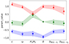 |
Fig. 9. Median values of the six dynamical state proxies for the subsamples of relaxed clusters (blue stars), intermediate clusters (green dots), and disturbed clusters (red triangles). The parameters are standardized using the STANDARDSCALER class from SCIKIT-LEARN. This scale corresponds to −3.30 ≤ param_value ≤ 2.60, where param_value is the dimensionless scaled value of any dynamical parameter. The concentration parameter c is inverted for visualization purposes only. The shaded areas and error bars represent the 1σ regions. |
7. Discussion and conclusions
7.1. Brightest cluster galaxy selection accuracy
As we mention in Section 4, we employed an automatic method to select the BCG candidates of all the galaxy clusters in the sample. However, we used visual inspection to ensure that the selection was correct; namely, to confirm or reject the BCG candidates selected with the automatic method. In 70% of the cases, the BCG selected by both methods coincides. For the remaining cases, we attribute the error of the automatic method to three main reasons; the cluster membership method used, the specific physical processes that can occur, and special cases. Specifically, the first is that the method of assigning members using photometric redshifts has a contamination rate that can reach 25%, and this can cause a redder galaxy than the BCG to be found within the 1σ region of the best fit of the red sequence, which does not actually belong to the cluster. The second reason is due to the presence of cooling flows in relaxed clusters, where the cold gas directly reaches the BCG, triggering significant star formation and/or nuclear activity (e.g., Rawle et al. 2012). This causes the BCG to be bluer and, therefore, might not be selected by the automatic method. Regarding special cases, it is possible for a spectroscopic confirmed member galaxy within R200 to be brighter than the BCG. An example of this is the galaxy cluster Abell 3827, where four galaxies in the central region are likely to merge into a dominant central galaxy (cD) in the future (Carrasco et al. 2010). However, at the time of observation, this has not yet occurred, and another galaxy that is brighter than any of the four central ones does exist, but it does not meet the other criteria for classification as the BCG (Carrasco et al., in prep.).
Even more importantly, since we are measuring the accuracy of the automatic method with respect to visual inspection, we must ensure that the selection of the BCG using the latter method is indeed correct. To this end, we have spectroscopic information from the literature (Table 1). In Fig. 10, we present as an example the peculiar velocities of six galaxy clusters from the sample within the range of ±6000 km s−1, and we observe that all the BCGs selected visually indeed belong to the cluster. This occurs for the 30 systems for which we have spectroscopic information for the BCG selected by visual inspection, which gives us confidence in the method.
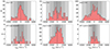 |
Fig. 10. Peculiar velocity distributions of galaxies within 6000 km s−1 of six example galaxy clusters. The members are marked with red bars. The black dashed lines indicate the positions of the BCGs selected by visual inspection. The shaded areas represent the 1σ, 2σ, and 3σ regions from darkest to lightest. The cluster names are indicated in the upper left corners of each panel. The bin sizes are 250 km s−1. |
It is important to clarify that the accuracy of the automatic method does not have any effect on the results of this work, because, as we previously said, the candidates for the BCG were then confirmed or rejected by visual inspection and spectroscopic redshifts when available. We provide the accuracy of the method only as a reference to take into account what can be improved in future works.
7.2. Dynamical parameters
Although classifying dynamical states based on a single parameter can help to distinguish the most extreme cases, a proper combination of these indices can be more robust. To quantify this aspect, we compared our results with those obtained by Yuan & Han (2020) and Yuan et al. (2022). For disturbed clusters, we find consistent results between our classification system and that used by Yuan & Han (2020) and Yuan et al. (2022) (δ > 0). However, we note a discrepancy for the relaxed clusters. Of the 32 relaxed galaxy clusters in our sample, 13 do not fall into this category according to the Yuan & Han (2020) and Yuan et al. (2022) criteria (δ < 0)7. This fraction corresponds to 40%, and since this is a rather high value, we have individually analyzed these 13 systems. They all have a wbs value of −0.0057, which is almost at the threshold of our separation between relaxed and intermediate clusters. However, upon inspection, only Abell 3322, Abell 3783, and MCXCJ0528.9-3927 exhibit interaction features typical of an unrelaxed cluster (see the figures on Zenodo8). This indicates the need for an intermediate systems category rather than opting for a binary classification between relaxed and disturbed clusters and our combined use of dynamical state proxies allows us to do this robustly.
The binary separation between relaxed and disturbed clusters arises from the bimodalities found in the distributions of these dynamical parameters. However, in some cases, the bimodalities may be absent, making the classification task more challenging (e.g., Campitiello et al. 2022). The use of two dynamical state proxies together in a two-dimensional (2D) parameter space has been shown to aid in this classification task (e.g., Cassano et al. 2010, 2013). However, even more robust results can be obtained by combining multiple dynamical parameters, such as with the M statistic (e.g., Rasia et al. 2013; Lovisari et al. 2017). In our case, we have chosen to use PCA with our set of six proxies, finding that the first principal component can effectively separate the dynamical states of the clusters, which is consistent with Campitiello et al. (2022).
7.3. Classification of dynamical states
From our total sample of 87 galaxy clusters, we classified 32 (∼36%) as relaxed clusters, 30 (∼34%) as systems with an intermediate dynamical state, and 25 (∼29%) as disturbed clusters of galaxies. Thus, we identified a fraction of ∼63% of galaxy clusters in an unrelaxed state (intermediate and disturbed), which is consistent with the expected range of 30 − 80% according to previous studies (e.g., Dressler & Shectman 1988; Santos et al. 2008; Fakhouri et al. 2010; Wen & Han 2013; Yuan & Han 2020; Yuan et al. 2022). This sample will then be our starting point in Paper II to study the effect of the dynamical state of galaxy clusters on their populations, focusing on the physical and structural properties of member galaxies.
Data availability
We provide three figures via Zenodo at https://zenodo.org/records/14241676, showing the contours of the X-ray surface brightness distribution, the distribution of red sequence galaxies, and the positions of the BGGs, X-ray peaks, and X-ray centroids.
Completeness and contamination are calculated by selecting a membership probability threshold based on photometric data, and these values are obtained by comparison with spectroscopic data and assumed for the entire sample.
The K-corrections are applied to the CSP that models the evolution of m*. As a result, the same m*, specific to each cluster and already incorporating the K-correction, is used for all galaxies within that cluster, regardless of their morphology.
This subsample of clusters corresponds to Abell 122, Abell 223, Abell 3322, Abell 3364, Abell 3718, Abell 3783, MCXC J0528.9-3927, PLCKESZG256.4-65, PLCKG334.8-38.0A, RXC J0439.2-4600, RXC J0528.2-2942, SPT-CLJ0106-5943, and SPT-CLJ2130-6458.
Acknowledgments
JLNC & SVA acknowledges the financial support of DIDULS/ULS, through the Proyecto Apoyo de Tesis de Postgrado N° PTE2353858. ERC acknowledges the support of the International Gemini Observatory, a program of NSF NOIRLab, which is managed by the Association of Universities for Research in Astronomy (AURA) under a cooperative agreement with the U.S. National Science Foundation, on behalf of the Gemini partnership of Argentina, Brazil, Canada, Chile, the Republic of Korea, and the United States of America. We wish to thank the anonymous referee for a constructive report that helped us improve our manuscript.
References
- Abbott, T. M. C., Adamów, M., Aguena, M., et al. 2021, ApJS, 255, 20 [NASA ADS] [CrossRef] [Google Scholar]
- Aldás, F., Zenteno, A., Gómez, F. A., et al. 2023, MNRAS, 525, 1769 [CrossRef] [Google Scholar]
- Andreon, S. 2006, A&A, 448, 447 [NASA ADS] [CrossRef] [EDP Sciences] [Google Scholar]
- Baldry, I. K., Glazebrook, K., Brinkmann, J., et al. 2004, ApJ, 600, 681 [Google Scholar]
- Balogh, M. L., Baldry, I. K., Nichol, R., et al. 2004, ApJ, 615, L101 [Google Scholar]
- Bayliss, M. B., Hennawi, J. F., Gladders, M. D., et al. 2011, ApJS, 193, 8 [Google Scholar]
- Bayliss, M. B., Ruel, J., Stubbs, C. W., et al. 2016, ApJS, 227, 3 [NASA ADS] [CrossRef] [Google Scholar]
- Beers, T. C., Flynn, K., & Gebhardt, K. 1990, AJ, 100, 32 [Google Scholar]
- Blum, R. D., Burleigh, K., Dey, A., et al. 2016, Am. Astron. Soc. Meet. Abstr., 228, 317.01 [Google Scholar]
- Boschin, W., Girardi, M., & Barrena, R. 2013, MNRAS, 434, 772 [NASA ADS] [CrossRef] [Google Scholar]
- Bouwens, R. J., Bradley, L., Zitrin, A., et al. 2014, ApJ, 795, 126 [Google Scholar]
- Braglia, F. G., Pierini, D., Biviano, A., & Böhringer, H. 2009, A&A, 500, 947 [NASA ADS] [CrossRef] [EDP Sciences] [Google Scholar]
- Brunner, R. J., & Lubin, L. M. 2000, AJ, 120, 2851 [NASA ADS] [CrossRef] [Google Scholar]
- Bruzual, A. G. 1983, ApJ, 273, 105 [CrossRef] [Google Scholar]
- Bruzual, G., & Charlot, S. 2003, MNRAS, 344, 1000 [NASA ADS] [CrossRef] [Google Scholar]
- Buote, D. A., & Tsai, J. C. 1995, ApJ, 452, 522 [Google Scholar]
- Campitiello, M. G., Ettori, S., Lovisari, L., et al. 2022, A&A, 665, A117 [NASA ADS] [CrossRef] [EDP Sciences] [Google Scholar]
- Carrasco, E. R., Gomez, P. L., Verdugo, T., et al. 2010, ApJ, 715, L160 [NASA ADS] [CrossRef] [Google Scholar]
- Carrasco, E. R., Verdugo, T., Motta, V., et al. 2021, ApJ, 918, 61 [NASA ADS] [CrossRef] [Google Scholar]
- Cassano, R., Ettori, S., Giacintucci, S., et al. 2010, ApJ, 721, L82 [Google Scholar]
- Cassano, R., Ettori, S., Brunetti, G., et al. 2013, ApJ, 777, 141 [Google Scholar]
- Clowe, D., Bradač, M., Gonzalez, A. H., et al. 2006, ApJ, 648, L109 [NASA ADS] [CrossRef] [Google Scholar]
- Cuciti, V., Cassano, R., Brunetti, G., et al. 2021, A&A, 647, A50 [NASA ADS] [CrossRef] [EDP Sciences] [Google Scholar]
- de Albernaz Ferreira, L., & Ferrari, F. 2018, MNRAS, 473, 2701 [CrossRef] [Google Scholar]
- de Los Rios, M., Domínguez R., M. J., Paz, D., & Merchán, M. 2016, MNRAS, 458, 226 [NASA ADS] [CrossRef] [Google Scholar]
- De Lucia, G., Poggianti, B. M., Aragón-Salamanca, A., et al. 2004, ApJ, 610, L77 [NASA ADS] [CrossRef] [Google Scholar]
- de Propris, R., Stanford, S. A., Eisenhardt, P. R., Dickinson, M., & Elston, R. 1999, AJ, 118, 719 [NASA ADS] [CrossRef] [Google Scholar]
- Dey, A., Schlegel, D. J., Lang, D., et al. 2019, AJ, 157, 168 [Google Scholar]
- Dressler, A., & Shectman, S. A. 1988, AJ, 95, 985 [Google Scholar]
- Drlica-Wagner, A., Ferguson, P. S., Adamów, M., et al. 2022, ApJS, 261, 38 [NASA ADS] [CrossRef] [Google Scholar]
- Duncan, K. J. 2022, MNRAS, 512, 3662 [NASA ADS] [CrossRef] [Google Scholar]
- Fabian, A. C., Johnstone, R. M., & Daines, S. J. 1994, MNRAS, 271, 737 [NASA ADS] [CrossRef] [Google Scholar]
- Fakhouri, O., Ma, C.-P., & Boylan-Kolchin, M. 2010, MNRAS, 406, 2267 [Google Scholar]
- Foëx, G., Chon, G., & Böhringer, H. 2017, A&A, 601, A145 [NASA ADS] [CrossRef] [EDP Sciences] [Google Scholar]
- Geller, M. J., Hwang, H. S., Diaferio, A., et al. 2014, ApJ, 783, 52 [NASA ADS] [CrossRef] [Google Scholar]
- Golovich, N., Dawson, W. A., Wittman, D. M., et al. 2019, ApJS, 240, 39 [NASA ADS] [CrossRef] [Google Scholar]
- Guzzo, L., Schuecker, P., Böhringer, H., et al. 2009, A&A, 499, 357 [NASA ADS] [CrossRef] [EDP Sciences] [Google Scholar]
- Harvey, D., Massey, R., Kitching, T., Taylor, A., & Tittley, E. 2015, Science, 347, 1462 [Google Scholar]
- Hinshaw, G., Larson, D., Komatsu, E., et al. 2013, ApJS, 208, 19 [Google Scholar]
- Hotelling, H. 1933, J. Educ. Psychol., 24, 417 [CrossRef] [Google Scholar]
- Huber, P., & Ronchetti, E. 2011, Robust Statistics, WileySeries in Probability and Statistics (Wiley) [Google Scholar]
- Jee, M. J., Hoekstra, H., Mahdavi, A., & Babul, A. 2014, ApJ, 783, 78 [NASA ADS] [CrossRef] [Google Scholar]
- Jeltema, T. E., Canizares, C. R., Bautz, M. W., & Buote, D. A. 2005, ApJ, 624, 606 [Google Scholar]
- Kesebonye, K. C., Hilton, M., Knowles, K., et al. 2023, MNRAS, 518, 3004 [Google Scholar]
- Kravtsov, A. V., & Borgani, S. 2012, ARA&A, 50, 353 [Google Scholar]
- Lang, D., Hogg, D. W., & Mykytyn, D. 2016, Astrophysics Source Code Library [record ascl:1604.008] [Google Scholar]
- Lovisari, L., Forman, W. R., Jones, C., et al. 2017, ApJ, 846, 51 [Google Scholar]
- Mancone, C. L., & Gonzalez, A. H. 2012, PASP, 124, 606 [NASA ADS] [CrossRef] [Google Scholar]
- Mann, A. W., & Ebeling, H. 2012, MNRAS, 420, 2120 [NASA ADS] [CrossRef] [Google Scholar]
- Markevitch, M., Gonzalez, A. H., David, L., et al. 2002, ApJ, 567, L27 [Google Scholar]
- McDonald, M., Bayliss, M., Benson, B. A., et al. 2012, Nature, 488, 349 [Google Scholar]
- McDonald, M., Benson, B. A., Vikhlinin, A., et al. 2013, ApJ, 774, 23 [NASA ADS] [CrossRef] [Google Scholar]
- Menci, N., Fontana, A., Giallongo, E., & Salimbeni, S. 2005, ApJ, 632, 49 [NASA ADS] [CrossRef] [Google Scholar]
- Mercurio, A., Rosati, P., Biviano, A., et al. 2021, A&A, 656, A147 [NASA ADS] [CrossRef] [EDP Sciences] [Google Scholar]
- Molnar, S. M. 2016, Front. Astron. Space Sci., 2, 7 [NASA ADS] [CrossRef] [Google Scholar]
- Nilo Castellón, J. L., Alonso, M. V., García Lambas, D., et al. 2014, MNRAS, 437, 2607 [CrossRef] [Google Scholar]
- Nurgaliev, D., McDonald, M., Benson, B. A., et al. 2013, ApJ, 779, 112 [NASA ADS] [CrossRef] [Google Scholar]
- Okabe, N., Takada, M., Umetsu, K., Futamase, T., & Smith, G. P. 2010, PASJ, 62, 811 [NASA ADS] [Google Scholar]
- Owers, M. S., Randall, S. W., Nulsen, P. E. J., et al. 2011, ApJ, 728, 27 [Google Scholar]
- Owers, M. S., Nulsen, P. E. J., Couch, W. J., et al. 2014, ApJ, 780, 163 [Google Scholar]
- Pelló, R., Rudnick, G., De Lucia, G., et al. 2009, A&A, 508, 1173 [NASA ADS] [CrossRef] [EDP Sciences] [Google Scholar]
- Poole, G. B., Fardal, M. A., Babul, A., et al. 2006, MNRAS, 373, 881 [Google Scholar]
- Proust, D., Cuevas, H., Capelato, H. V., et al. 2000, A&A, 355, 443 [NASA ADS] [Google Scholar]
- Rasia, E., Meneghetti, M., & Ettori, S. 2013, Astron. Rev., 8, 40 [Google Scholar]
- Rawle, T. D., Edge, A. C., Egami, E., et al. 2012, ApJ, 747, 29 [NASA ADS] [CrossRef] [Google Scholar]
- Ribeiro, A. L. B., Lopes, P. A. A., & Rembold, S. B. 2013, A&A, 556, A74 [NASA ADS] [CrossRef] [EDP Sciences] [Google Scholar]
- Richard, J., Claeyssens, A., Lagattuta, D., et al. 2021, A&A, 646, A83 [EDP Sciences] [Google Scholar]
- Rines, K., Geller, M. J., Diaferio, A., & Kurtz, M. J. 2013, ApJ, 767, 15 [NASA ADS] [CrossRef] [Google Scholar]
- Ruel, J., Bazin, G., Bayliss, M., et al. 2014, ApJ, 792, 45 [NASA ADS] [CrossRef] [Google Scholar]
- Santos, J. S., Rosati, P., Tozzi, P., et al. 2008, A&A, 483, 35 [NASA ADS] [CrossRef] [EDP Sciences] [Google Scholar]
- Sifón, C., Battaglia, N., Hasselfield, M., et al. 2016, MNRAS, 461, 248 [CrossRef] [Google Scholar]
- Silva, D. R., Blum, R. D., Allen, L., et al. 2016, Am. Astron. Soc. Meet. Abstr., 228, 317.02 [NASA ADS] [Google Scholar]
- Skillman, S. W., Xu, H., Hallman, E. J., et al. 2013, ApJ, 765, 21 [Google Scholar]
- Stalder, B., Ruel, J., Šuhada, R., et al. 2013, ApJ, 763, 93 [NASA ADS] [CrossRef] [Google Scholar]
- The Dark Energy Survey Collaboration 2005, ArXiv e-prints [arXiv:astro-ph/0510346] [Google Scholar]
- Thompson, R., Davé, R., & Nagamine, K. 2015, MNRAS, 452, 3030 [NASA ADS] [CrossRef] [Google Scholar]
- Tucker, E., Walker, M. G., Mateo, M., et al. 2017, AJ, 154, 113 [NASA ADS] [CrossRef] [Google Scholar]
- Umetsu, K., Medezinski, E., Nonino, M., et al. 2014, ApJ, 795, 163 [NASA ADS] [CrossRef] [Google Scholar]
- Vikhlinin, A., Kravtsov, A., Forman, W., et al. 2006, ApJ, 640, 691 [Google Scholar]
- Voit, G. M. 2005, Rev. Mod. Phys., 77, 207 [Google Scholar]
- Vulcani, B., Poggianti, B. M., Fasano, G., et al. 2012, MNRAS, 420, 1481 [NASA ADS] [CrossRef] [Google Scholar]
- Wen, Z. L., & Han, J. L. 2013, MNRAS, 436, 275 [Google Scholar]
- Wen, Z. L., & Han, J. L. 2015, ApJ, 807, 178 [Google Scholar]
- Wen, Z. L., & Han, J. L. 2021, MNRAS, 500, 1003 [Google Scholar]
- Wen, Z. L., & Han, J. L. 2022, MNRAS, 513, 3946 [NASA ADS] [CrossRef] [Google Scholar]
- Wright, E. L., Eisenhardt, P. R. M., Mainzer, A. K., et al. 2010, AJ, 140, 1868 [Google Scholar]
- Yuan, Z. S., & Han, J. L. 2020, MNRAS, 497, 5485 [Google Scholar]
- Yuan, Z. S., Han, J. L., & Wen, Z. L. 2022, MNRAS, 513, 3013 [NASA ADS] [CrossRef] [Google Scholar]
- Zenteno, A., Mohr, J. J., Desai, S., et al. 2016, MNRAS, 462, 830 [NASA ADS] [CrossRef] [Google Scholar]
- Zenteno, A., Hernández-Lang, D., Klein, M., et al. 2020, MNRAS, 495, 705 [Google Scholar]
- Zhang, Y.-Y., Okabe, N., Finoguenov, A., et al. 2010, ApJ, 711, 1033 [NASA ADS] [CrossRef] [Google Scholar]
- Zou, H., Zhou, X., Fan, X., et al. 2017, PASP, 129, 064101 [CrossRef] [Google Scholar]
Appendix A: Full cluster catalog
Relevant information about the full sample of galaxy clusters. Columns: (1) galaxy cluster name; (2-3) right ascension and declination in J2000; (4) redshift; (5) characteristic magnitude in the r-band; (6) R200 in Mpc; (7) M200 in 1044M/M⊙ units; (8) cluster member galaxies using photometric redshifts; (9) concentration; (10) centroid shift; (11) power ratio; (12) morphological parameter; (13) BCG/X-ray peak offset in kpc; (14) BCG/X-ray centroid offset in kpc; (15) dynamical state.
Appendix B: Radar charts of the dynamical state proxies
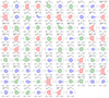 |
Fig. B.1. Radar charts with the six dynamical parameters used in this work for all clusters in the sample. The colors blue, green, and red indicate the relaxed, intermediate, and disturbed dynamical states, respectively. The parameter values are scaled in the same way as in Fig. 9. |
All Tables
Galaxy clusters with known dynamical states from literature used to calibrate our method.
Normalized statistical weight of the dynamical parameters associated with the first principal component.
Relevant information about the full sample of galaxy clusters. Columns: (1) galaxy cluster name; (2-3) right ascension and declination in J2000; (4) redshift; (5) characteristic magnitude in the r-band; (6) R200 in Mpc; (7) M200 in 1044M/M⊙ units; (8) cluster member galaxies using photometric redshifts; (9) concentration; (10) centroid shift; (11) power ratio; (12) morphological parameter; (13) BCG/X-ray peak offset in kpc; (14) BCG/X-ray centroid offset in kpc; (15) dynamical state.
All Figures
|
Fig. 1. Comparison of spectroscopic and photometric redshifts (zspec and zphot) and the normalized redshift deviation (Δznorm). Left: Comparison between zspec and zphot. The solid black line represents the identity line (zspec = zphot). Middle: Δznorm as function of zspec. Right: Δznorm as function of zspec. In the latter two cases, the solid black line corresponds to the constant function where Δznorm = 0. |
| In the text | |
|
Fig. 2. Fraction of retained members (completeness, black dots) and non-members (contamination, gray crosses) as a function of the probability threshold Pthreshold. This figure was created using only galaxies with secure zspec measurements in clusters with enough spectroscopic data for members and the field. |
| In the text | |
|
Fig. 3. Fraction of galaxies as function of the clustercentric distance for the stacked sample of galaxy clusters. Dark red points correspond to the median values in each bin, while the lower and upper error bars are the first and third quartile in each bin, respectively. |
| In the text | |
|
Fig. 4. Double Gaussian fits applied to the normalized color distribution of each cluster. From left to right panels, Abell 3827 (relaxed cluster), Abell 3739 (intermediate cluster), and Abell 2744 (disturbed cluster) are presented as examples. The colors of the Gaussians are associated with the red and blue components of the galaxy clusters. The black dashed line indicated the red_limit in each panel. The specific value of this parameter is located in the upper left corner of each panel along with the χ2 statistic for each fit performed with LMFIT. |
| In the text | |
|
Fig. 5. Normalized color-magnitude diagrams for the same clusters mentioned in Fig. 4. Black dots correspond to galaxies selected as members using the probabilistic method with photometric redshifts. Green triangles represent galaxies pre-selected as BCGs using the automated method, while purple inverted triangles denote visually confirmed BCGs. The solid red lines represent the best fits of the red sequences calculated with HuberRegressor and the red shaded areas are the 1σ regions of them. The vertical blue dashed lines indicate the magnitude limit for studying physical and structural properties, namely, m* + 3, where m* is the characteristic magnitude at each cluster redshift modeled with CPS. |
| In the text | |
|
Fig. 6. Correlation matrix of the six dynamical state proxies used in this work. The diagonal displays the kernel density estimation (KDE) of each variable. Below the diagonal, scatter plots with linear fits and their corresponding confidence intervals are presented for all combinations of these parameters. Above the diagonal, the Pearson correlation coefficients associated with each parameter space are shown. |
| In the text | |
|
Fig. 7. Parameter space of the first two principal components (PC 1 and PC 2) obtained from the six dynamic parameters described in Section 5 for the 26 clusters in the sample that have a well-defined dynamical state in the literature. Blue, red, and green symbols represent relaxed, disturbed, and intermediate clusters, respectively. Crosses, dots, squares and triangles correspond to the data extracted from Cassano et al. (2010), Cuciti et al. (2021), Kesebonye et al. (2023), and Lovisari et al. (2017), respectively. |
| In the text | |
|
Fig. 8. Distribution of the wbs parameter for all the galaxy clusters in the sample. We classify relaxed clusters as systems with wbs < 0 (blue bars), disturbed clusters with wbs > 0 (red bars), and the remaining clusters in between as an intermediate population of galaxy clusters (green bars). |
| In the text | |
|
Fig. 9. Median values of the six dynamical state proxies for the subsamples of relaxed clusters (blue stars), intermediate clusters (green dots), and disturbed clusters (red triangles). The parameters are standardized using the STANDARDSCALER class from SCIKIT-LEARN. This scale corresponds to −3.30 ≤ param_value ≤ 2.60, where param_value is the dimensionless scaled value of any dynamical parameter. The concentration parameter c is inverted for visualization purposes only. The shaded areas and error bars represent the 1σ regions. |
| In the text | |
|
Fig. 10. Peculiar velocity distributions of galaxies within 6000 km s−1 of six example galaxy clusters. The members are marked with red bars. The black dashed lines indicate the positions of the BCGs selected by visual inspection. The shaded areas represent the 1σ, 2σ, and 3σ regions from darkest to lightest. The cluster names are indicated in the upper left corners of each panel. The bin sizes are 250 km s−1. |
| In the text | |
|
Fig. B.1. Radar charts with the six dynamical parameters used in this work for all clusters in the sample. The colors blue, green, and red indicate the relaxed, intermediate, and disturbed dynamical states, respectively. The parameter values are scaled in the same way as in Fig. 9. |
| In the text | |
Current usage metrics show cumulative count of Article Views (full-text article views including HTML views, PDF and ePub downloads, according to the available data) and Abstracts Views on Vision4Press platform.
Data correspond to usage on the plateform after 2015. The current usage metrics is available 48-96 hours after online publication and is updated daily on week days.
Initial download of the metrics may take a while.