| Issue |
A&A
Volume 698, May 2025
|
|
|---|---|---|
| Article Number | A171 | |
| Number of page(s) | 10 | |
| Section | Extragalactic astronomy | |
| DOI | https://doi.org/10.1051/0004-6361/202452440 | |
| Published online | 11 June 2025 | |
The dynamical state of eROSITA clusters and its impact on the brightest cluster galaxy luminosity
1
Cerro Tololo Inter-American Observatory, NSF’s National Optical-Infrared Astronomy Research Laboratory, Casilla 603, La Serena, Chile
2
Max Planck Institute for Extraterrestrial Physics, Giessenbachstrasse 1, 85748 Garching, Germany
3
Université Paris-Saclay, CNRS, Institut d’Astrophysique Spatiale, 91405 Orsay, France
4
Max Planck Institute for Extraterrestrial Physics, Giessenbachstrasse 1, 85748 Garching, Germany
5
Faculty of Physics, Ludwig-Maximilians-Universität München, Scheinerstr. 1, 81679 Munich, Germany
6
INAF – Osservatorio Astronomico di Trieste, via G. B. Tiepolo 11, 34143 Trieste, Italy
7
IFPU – Institute for Fundamental Physics of the Universe, Via Beirut 2, 34014 Trieste, Italy
8
Astronomy Unit, Department of Physics, University of Trieste, via Tiepolo 11, 34131 Trieste, Italy
9
INFN – National Institute for Nuclear Physics, Via Valerio 2, I-34127 Trieste, Italy
10
ICSC – Italian Research Center on High Performance Computing, Big Data and Quantum Computing, Bologna, Italy
11
Institute of Astronomy and Astrophysics, Academia Sinica, Taipei 10617, Taiwan
12
International Gemini Observatory/NSF NOIRLab, Casilla 603, La Serena, Chile
13
Instituto de Física y Astronomía, Universidad de Valparaíso, Gran Bretaña 1111, Valparaíso, Chile
14
Millennium Nucleus on Transversal Research and Technology to Explore Supermassive Black Holes (TITANS), Valparaíso, Chile
15
Departamento de Astronomía, Universidad de La Serena, Av. Raúl Bitrán 1305, La Serena, Chile
16
Lawrence Berkeley National Laboratory, 1 Cyclotron Road, Berkeley, CA 94720, USA
17
Department of Physics and Astronomy, University of Wyoming, 1000 E. University, Dept. 3905, Laramie, WY 82071, USA
18
Space Telescope Science Institute, 3700 San Martin Drive, Baltimore, MD 21218, USA
19
NSF’s National Optical/Infrared Research Laboratory (NOIRLab), 950 N. Cherry Ave, Tucson AZ 85732, USA
20
Universität Innsbruck, Institut für Astro-und Teilchenphysik, Technikerstr. 25/8, 6020 Innsbruck, Austria
⋆ Corresponding author: alfredo.zenteno@noirlab.edu
Received:
1
October
2024
Accepted:
26
March
2025
Context. The first Spectrum-Roentgen-Gamma (SRG) eROSITA public release contains 12 247 clusters and groups from its first 6 months of operation. We used the offset between the brightest cluster galaxy (BCG) and the X-ray peak (DBCG − X) to classify the cluster dynamical state of 3946 galaxy clusters and groups.
Aims. We aim to investigate the evolution of the merger and relaxed cluster distributions with redshift and mass, and the distributions’ impact on the BCG.
Methods. We used the X-ray peak from the eROSITA survey and the BCG position from the LS DR10 optical data, which includes the DECam eROSITA Survey optical data, to measure the DBCG − X offset. We modelled the distribution of DBCG − X, in units of R500, as the sum of two Rayleigh distributions representing the cluster’s relaxed and disturbed populations, and explored their evolution with redshift and mass. To explore the impact of the cluster’s dynamical state on the BCG luminosity, we separated the main sample according to the dynamical state. We defined clusters as relaxed if DBCG − X < 0.25R500, disturbed if DBCG − X > 0.5R500, and ‘diverse’ if 0.25R500 < DBCG − X < 0.5R500.
Results. We find no evolution of the merging fraction with redshift or mass. The width of the relaxed distribution increases with redshift, while the width of the two Rayleigh distributions decreases with mass. The analysis reveals that BCGs in relaxed clusters are brighter than BCGs in both the disturbed and diverse cluster populations. The most significant differences are found for high-mass clusters at higher redshifts.
Conclusions. The results suggest that BCGs in low-mass clusters are less centrally bound than those in high-mass systems, irrespective of the dynamical state. Over time, BCGs in relaxed clusters progressively align with the potential centre. This alignment correlates with their luminosity growth relative to BCGs in dynamically disturbed clusters, underscoring the critical role of the cluster’s dynamical state in regulating BCG evolution.
Key words: galaxies: clusters: general
© The Authors 2025
 Open Access article, published by EDP Sciences, under the terms of the Creative Commons Attribution License (https://creativecommons.org/licenses/by/4.0), which permits unrestricted use, distribution, and reproduction in any medium, provided the original work is properly cited.
This article is published in open access under the Subscribe to Open model. Subscribe to A&A to support open access publication.
1. Introduction
The process governing the buildup of the Universe’s large-scale structure is hierarchical, with larger formations emerging from successive mergers of smaller entities (Nelson et al. 2024). Given the continuous nature of this process, galaxy clusters exist in various dynamical states, ranging from those already virialized to highly disturbed clusters still undergoing formation (e.g. Pandge et al. 2019; Lourenço et al. 2020; Yoon et al. 2020; Monteiro-Oliveira 2022; Abriola et al. 2024). Each evolutionary stage provides us with a different aspect of cluster science. For example, (almost) relaxed clusters are the most suitable targets for investigations of intracluster gas cooling and heating processes (e.g. Soja et al. 2018; Ueda et al. 2020, 2021; Hlavacek-Larrondo et al. 2022; Ruszkowski & Pfrommer 2023). They are also optimal for establishing scaling relations between different observables (e.g. Monteiro-Oliveira et al. 2021; Lovisari & Maughan 2022; Bahar et al. 2022; Chiu et al. 2023; Doubrawa et al. 2023), determining cluster counts for cosmology probes (Costanzi et al. 2021; Bocquet et al. 2024; Fumagalli et al. 2024; Ghirardini et al. 2024; Artis et al. 2024), and testing the validity of the Λ cold dark matter (CDM) model (Chan & Del Popolo 2020; Brouwer et al. 2021; Tam et al. 2023). Research topics that can be explored using disturbed clusters include how each cluster’s constituents (gas, galaxies, and dark matter) behave under extreme circumstances (e.g. Molnar 2016; Monteiro-Oliveira et al. 2022; Doubrawa et al. 2020; Moura et al. 2021; Albuquerque et al. 2024; Véliz Astudillo et al. 2025), the determination of the conditions for particle acceleration (e.g. Botteon et al. 2019), and tests of exotic forms of dark matter (e.g. Bulbul et al. 2014; Harvey et al. 2015; Fischer et al. 2023; Sirks et al. 2024).
While the impact of galaxy mass and/or environmental factors on galaxy properties is relatively well understood (e.g. Dressler 1980; Peng et al. 2010), the influence of processes at larger scales on the evolution of galaxies, such as highly energetic cluster mergers (up to 1064 erg; Sarazin 2004), remains unclear. Given that the most pronounced effects of cluster collisions (e.g. gas heating and shock propagation) occur within a few million years after the pericentric passage (e.g. Markevitch & Vikhlinin 2007; ZuHone 2011), during a period of significant dynamical disruption (e.g. Machado et al. 2015; Ruggiero et al. 2019), observations of young post-collision systems can offer ‘real-time’ insights into the potential effects on the stellar activity of the galaxies.
Pilot studies on individual mergers have found that the impact of mergers on the galaxy population can vary. For example, Hernández-Lang et al. (2022) analysed the merging cluster SPT-CL J0307-6225 using the Multi Unit Spectroscopic Explorer (MUSE) data. At redshift z = 0.58, they find that most of the emission-line galaxies lie close to the X-ray peak position; however, when separating by galaxy population, they find that a third of the emission-line galaxies correspond to red-sequence cluster galaxies. Moreover, these emission-line red-sequence galaxies were classified as short-starburst galaxies, which, based on the peculiar velocities, must have been accreted before the merger between the two clusters occurred. On the other hand, 75% of the blue emission-line galaxies have peculiar velocities, which suggests they are in the process of being accreted. The young (0.5 Gyr; Machado & Lima Neto 2013) binary merging cluster A3376 (z = 0.046; Monteiro-Oliveira et al. 2017) displays a pair of radio relics (Akamatsu et al. 2012) as a result of the shock propagating through the intracluster medium. Kelkar et al. (2020) conclude that this shock had distinct effects on high- and low-mass spiral galaxies. While the high-mass spirals were not significantly affected, and thus maintained stellar activity similar to that of the relaxed clusters, the stellar formation of the low-mass ones was suppressed due to the interaction between the clusters. A plausible scenario is that the impact of the merger is temporary and, therefore, more evident in extremely young systems. Wittman et al. (2024), in a recent analysis of the distribution of Hα emitters in 12 merging clusters, note a slight trend indicating that the density of star-forming galaxies in the central region is lower compared to other galaxies in systems observed within 0.2 Gyr of the pericentric passage. However, this inference relies on only three systems and therefore lacks sufficient statistical significance for validation.
In the quest to find compelling evidence, researchers have started to build larger samples and explore different dynamical state proxies. In the X-ray regime, Lourenço et al. (2023) analysed 52 X-ray-selected clusters in the redshift range 0.04–0.07 with different dynamical states to explore the effect of extreme ram pressure on the merging cluster’s galaxy population. In particular, they looked at the prevalence of jellyfish galaxies as a function of the cluster dynamical state but were unable to find a correlation between them. Wen & Han (2015) used an optical proxy to classify the cluster dynamical state of 2092 optically selected rich galaxy clusters within the redshift range 0.05 < z < 0.42. Their study explored the impact of a cluster’s dynamical state on the bright end of the luminosity function. They found the knee of the Schechter function (m*) to be fainter in relaxed clusters with respect to disturbed clusters and the brightest cluster galaxy (BCG) to be brighter. Zenteno et al. (2020, Z20 henceforth) used Sunyaev-Zeldovich (SZ), X-ray, and optical information to classify the dynamical state of clusters and to study its impact on the cluster’s luminosity function. Z20 used the offsets between the BCG and the SZ centroid and between the BCG and the X-ray peak to classify the dynamical state of 288 massive South Pole Telescope-SZ selected clusters (Bleem et al. 2015). Z20 find that, when studying galaxies of all colours, (i) the faint end of the luminosity function is steeper, (ii) m* is brighter, and (iii) the BCG is fainter for merging clusters than for relaxed clusters at z ≳ 0.5, most significantly at 0.5 × R200. Aldás et al. (2023) expanded this work by exploring the impact of mergers on the red sequence, finding that merging clusters have a broader red sequence in the same z ≳ 0.5 redshift range and no difference at lower redshifts. Both works show that at the top of the cluster mass function, at z ≳ 0.5, quenching happens in situ, while at lower redshifts quenching happens ex situ.
As the impact of the cluster dynamical state on galaxy populations starts to become clearer, efforts to both improve dynamical state proxies and enlarge cluster samples with dynamical state classification have been carried out. This includes theoretical (e.g. Cui et al. 2017; Capalbo et al. 2021; De Luca et al. 2021) as well as observational work (e.g. Yuan & Han 2020). In particular, Yuan & Han (2020) used archival Chandra data of 964 clusters to explore new dynamical state proxies. They used the concentration index (c), the centroid shift (w), and the power ratio to create two of their own proxies: a profile parameter and an asymmetry factor. They find that these new proxies are excellent indicators for classifying a cluster’s dynamical state. In a follow-up study, Yuan et al. (2022) expanded the sample using 1308 XMM and 22 new Chandra X-ray data clusters, increasing the sample size to 1844 clusters; they find an agreement between the XMM and Chandra data. Other studies on X-ray-selected samples utilized data from the extended ROentgen Survey with an Imaging Telescope Array (eROSITA) aboard the Spectrum-Roentgen-Gamma (SRG) spacecraft (Merloni et al. 2012; Predehl et al. 2021; Merloni et al. 2024). Ghirardini et al. (2022) analysed X-ray data from eROSITA to measure eight morphological parameters for 325 galaxy clusters and groups (Liu et al. 2022). This dataset, covering approximately 140 deg2 from the eROSITA Final Equatorial-Depth Survey (eFEDS), shows that the fraction of relaxed objects is around 30–35%; no evidence of redshift evolution was found.
Another commonly used proxy for classifying the dynamical state of a large number of galaxy clusters is the BCG-X-ray peak–centroid offset (DBCG − X). This metric has been widely adopted as a reliable indicator of a cluster’s dynamical state (e.g. Mann & Ebeling 2012; Song et al. 2012; Lopes et al. 2018; Zenteno et al. 2020). The DBCG − X reflects the expectation that the collisionless BCG aligns with the bottom of the dark matter potential, while the collisional gas is displaced relative to the dark matter and galaxy components. Moreover, since this method relies on shallow optical and X-ray imaging, it enables measurements to be conducted without a substantial investment of telescope time per cluster.
In this work we go further and provide a dynamical state classification for 3946 uniformly X-ray-selected clusters. We used a sample of clusters and groups from the first eROSITA All-Sky Survey (eRASS1; Bulbul et al. 2024; Kluge et al. 2024) and combined that information with optical data from the Legacy Survey Data Release (DR) 10 (Dey et al. 2019), which includes the DECam eROSITA Survey (DeROSITAS). We used the dynamical state information to understand its impact on the BCG.
In Sect. 2.1 we introduce the X-ray data and cluster sample. In Sect. 2.2 we describe the optical data and the BCG selection we used paired with the X-ray data. In Sect. 2.4 we explore the BCG–X-ray offset distribution (DBCG − X). In Sect. 2.5 we use the DBCG − X to classify the cluster dynamical state, provide examples, and analyse the luminosity offset between the BCG luminosity and m* at the cluster redshift. Finally, in Sect. 3 we present our conclusions. Throughout this work we assume a flat ΛCDM cosmology with H0 = 68.3 km s−1 Mpc−1 and ΩM = 0.299 (Bocquet et al. 2015).
2. Data
2.1. eRASS1 X-ray data
The data from eRASS1 (Merloni et al. 2024) were collected between December 2019 and June 2020, and cover the western Galactic hemisphere (Galactic longitude 359.9442° > l > 179.9442°) with variable exposure time. In equatorial coordinates, this primarily corresponds to the southern sky. With a moderate angular resolution of ∼30″, galaxy clusters are resolved as extended sources, though 8347 clusters of galaxies have been identified in the point-sources catalogue (Balzer et al. 2025). The X-ray positional uncertainty is described by RADEC_ERR. RADEC_ERR corresponds to the sum of the errors in RA and Declination in quadrature, which for point sources 99% are within 10″ (Merloni et al. 2024).
The eRASS1-identified galaxy cluster catalogue (Bulbul et al. 2024; Kluge et al. 2024) contains 12 247 clusters and groups that were first selected in the X-ray and then identified at optical and near-infrared wavelengths. The latter step made use of the source catalogues from legacy surveys DR9 and DR10, which exclude the Galactic plane (Galactic latitude |b|≲20°) and thereby reduce the usable eRASS1 survey area to 13 116 deg2.
Cluster candidates are optically identified when at least two galaxies are found at any given redshift and the richness of the cluster candidate is λ > 3. For this procedure, the tool eROMaPPer (Ider Chitham et al. 2020) is used, which is based on the redMaPPer algorithm (Rykoff et al. 2012, 2014, 2016).
The X-ray properties of the eRASS1 galaxy clusters are published in Bulbul et al. (2024) and the optical properties in Kluge et al. (2024, K24 henceforth). The catalogue has a known statistical contamination of  . Most of these contaminants have a low richness and either a low or high redshift. We limited our analysis to a higher-quality subsample by applying further constraints:
-
The redshift of the cluster is greater than z = 0.05 (BEST_Z > 0.05),
-
The photometric redshift is smaller than the local limiting redshift (IN_ZVLIM=True),
-
The normalized richness is greater than 16 (LAMBDA_NORM > 16), corresponding to clusters with mass M200m ≳ 1014 M⊙,
-
The probability of the cluster being a contaminant is less than 10% (PCONT < 0.1),
-
The fraction of the cluster area masked is under 10% (MASKFRAC < 0.1),
-
The cluster mass is measured M500 > 1014 M⊙, and
-
R500 > 0.
These selection criteria reduce the number of clusters in our sample to 4303. We apply a further criterion on the quality of the BCG choice in Sect. 2.3. The final sample has a purity of 98% (1-PCONT = 0.98). As the X-ray centre, we used the refined measurement RA_XFIT and DEC_XFIT in Bulbul et al. (2024).
2.2. Optical data: LS DR10 and DeROSITAS
For the BCG position and brightness, K24 used the Legacy Survey (LS) DR9 and DR10 public release1 (Dey et al. 2019). DR10 was compiled using data from several programmes, large and small, to fill the extragalactic sky, covering a large fraction of the western galactic hemisphere. Among those programmes, most notably are the Legacy Survey DR9, the Dark Energy Survey (DES; Abbott et al. 2018), The DECam Local Volume Exploration Survey (DELVE; Drlica-Wagner et al. 2022)2, and the DECam eROSITA Survey (DeROSITAS; PI: Zenteno)34. In particular, our team designed DeROSITAS to fill the German eROSITA extragalactic sky to a griz minimum depth of 22.7 (23.5), 23.2 (24.0), 23.3 (24.0), and 22.5 (23.2) AB magnitudes at 10(5)σ, respectively. The goal was to reach a depth of m* + 1 at z ∼ 0.9 to obtain precise cluster photometric redshifts (see, for example, Song et al. 2012; Klein et al. 2017, 2019), a key ingredient to realize eROSITA cluster cosmology (Ghirardini et al. 2024). DeROSITAS dedicated about 100 nights using the Dark Energy Camera (DECam; Flaugher et al. 2015) on the Cerro Tololo Inter-American Observatory Blanco 4m telescope, between the 2017A and 2022A semesters, to ‘fill’ over 13 411 deg2 of extragalactic eROSITA-DE sky. DeROSITAS defined extragalactic eROSITA-DE sky as the sky excluding areas at decl. ≳ +30, with high Galactic hydrogen column density (NH > 1021 cm−2), a high density of stars (> 30 000 stars/deg2), or strong Galactic dust reddening (E(B − V) > 0.3 mag). Observations were carried out using the Legacy Survey tiling scheme with the 4 dithering pattern used by the DELVE-WIDE survey (Drlica-Wagner et al. 2021). DeROSITAS used the effective exposure timescale factor, teff (Neilsen et al. 2016) to repeat any observations with a teff of less than 0.20 (meaning the observation was equivalent to a 20% exposure time of the sky at the zenith on a dark night under ideal conditions). The use of teff also allowed DeROSITAS to adjust the required exposure time in a night by night basis; the total exposure time needed to reach full depth per pointing was estimated ( ) and distributed among the remaining dithered observing scripts, just before a DeROSITAS observing night. To reach a homogeneous depth, DeROSITAS observed no more than one dither per night. As at the time multiple surveys and programmes were covering the southern sky, DeROSITAS worked in coordination with other principle investigators to avoid duplication of efforts (e.g. DELVE). Information about the proposals and the data obtained can be found in Table 1.
DeROSITAS observations.
LS uses the community pipeline reduced data (Valdes et al. 2014), and The Tractor (Lang et al. 2016)5 to perform the source photometry. The Tractor used forward-modelling to perform source extraction on pixel-level data, modelling observed images as intrinsic profiles convolved with the point-spread function of each image. DR10 intrinsic profiles include six morphological types: point sources (PSF), round exponential galaxies with a variable radius (REX), de Vaucouleurs (DEV) profiles for elliptical galaxies, exponential (EXP) profiles for spiral galaxies, Sérsic (SER) profiles, and DUP for Gaia sources coincident with extended sources (no flux is reported for this type). Those models are fitted to the data at the pixel level, simultaneously modelling all individual images overlapping a source. For photometry we used magg, magr, magi, and magz while filtering out objects with type PSF, DUP, and negative flux in any band. Source morphological parameters are held fixed between the different filters, while source fluxes are allowed to vary between filters but are held constant in time. LS astrometry is fully aligned with Gaia DR 2 (Gaia Collaboration 2016; Lindegren et al. 2018), achieving astrometric residuals that are typically within ±0.03″.
2.3. BCG selection
Each K24 BCG was selected as the brightest cluster member based on its z-band magnitude. We verified that this selection is independent of the choice of filter. Shifting the selection wave band to the filter redwards of the 4000 Å break would result in consistent BCG choices in 98% of the cases.
The search radius around the X-ray detection is the cluster radius, Rλ (Rykoff et al. 2014, K24):

Nine-parameter model for the DBCG − X and DOPT − X offsets.
K24 expect that the BCG choice is consistent in only 80 ∼ 85% of the cases with other selection criteria based on the presence of diffuse intracluster light or visual inspection. To further clean our cluster sample, we visually inspected all 4303 clusters and, assuming a conservative approach, excluded the ∼8% of BCGs that are evidently wrong. ‘Evidently wrong’ BCGs includes, for example, cases where we find a larger and brighter galaxy, clearly visible close to the X-ray peak. Reasons for this selection error may include star-formation, dust absorption, or erroneous photometric measurements due to the BCG’s extended outer component. Those features could move the BCG off the red sequence. There are a couple cases where one entry had information from two overlapping clusters with the BCG of one cluster and the R500 from the other one, rendering an erroneous large DBCG − X offset (for example, 1eRASSJ033101.2-522843). Those rare cases are described in Appendix A.3 in K24 where the best redshift type was changed to a literature redshift, becoming unreliable. This reduces the BCG sample to 3946, which we used for our analysis. As an alternative proxy for the cluster centre, we also used the optical centre RA_OPT and DEC_OPT in K24 to compare to previous results found in Seppi et al. (2023). RA_OPT and DEC_OPT correspond to the most probable cluster centre found by a Bayesian classification algorithm (Rykoff et al. 2014; Seppi et al. 2023).
2.4. BCG-X-ray offset distribution
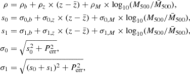
Following previous works (Saro et al. 2015, Z20), we characterized the offset distribution as the sum of two contributions, one describing the cluster population with small DBCG − X and the other with large DBCG − X. In particular, we fitted a model that assumes that both the well-centred and disturbed populations are described by a Rayleigh distribution:
where x = r/R500, and ρ (1 − ρ) is the fraction of well-centred (disturbed) clusters with a variance of σ02 (σ12).
The large number of clusters allows us to explore the mass and redshift evolution. We thus divided the cluster sample into 35 mass and redshift bins (to obtain about 100 clusters per bin) using a K-means algorithm. In each individual bin, we thus fitted the previously described miscentring model. As an example, we show in Fig. 1 the mass and redshift distribution of the analysed cluster catalogue, where each of the analysed bins has been colour-coded according to the resulting best-fit parameters derived within our model.
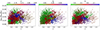 |
Fig. 1. Best-fit ρ, σ0, and σ1 parameters in bins of mass and redshift derived from Eq. (2). For σ, trends with both redshift and mass are observed. |
15 of the most relaxed eRASS1 clusters and groups.
15 of the most disturbed eRASS1 clusters and groups.
Figure 2 shows the marginalized posterior for each parameter as a function of the redshift and mean mass of the parent bin6. The fraction of well-centred clusters (described by the parameter ρ), does not appear to be significantly evolving with either mass or redshift. The trends highlighted by this figure are a correlation of σ0 with redshift and an anti-correlation with cluster mass, and an anti-correlation of σ1 with cluster mass. In other words, well-centred clusters have a tendency of being more disturbed at higher redshift, while smaller mass clusters (groups) have a tendency of having poorly centred BCGs (possibly due to their shallower potential well).
 |
Fig. 2. Marginalized distribution for ρ, σ0, and σ1 as a function of the mean redshift and mean mass of each analysed bin derived with Eq. (2). The fraction of (un)relaxed clusters (1 − ρ) ρ remains constant across redshifts, while we find a positive correlation of σ0 with redshift and a negative correlation of σ1 with mass. |
To more closely examine these results, which are characterized by the apparent linear dependence of σ0 and σ1 on redshift and (log) mass highlighted by Fig. 2, we expanded our model to allow mass and redshift dependence, including the X-ray peak positional error Perr (RADEC_ERR; Merloni et al. 2024), as follows:
where  and
and  are the median redshift and M500, use flat priors for 0 ≤ ρ ≤ 1, σ0 > 0, and s1 > 0 and Perr in R500 units. Perr evolves with redshift as it becomes a larger fraction of R500 at higher redshift. Figure 3 shows the resulting posterior distribution for our expanded model (Bocquet & Carter 2016), confirming what is seen in Fig. 2 (a positive redshift slope for σ0, z and a negative mass slope for σ0, M and ΔσM). This confirms that well-centred clusters seem to have a broader DBCG − X distribution at higher redshifts, while lower-mass clusters tend to have a broader DBCG − X distribution than their higher-mass counterparts.
 |
Fig. 3. Marginalized distribution of the miscentring model described by Eqs. (2) and (3). σ0 has a positive correlation with redshift ( |


Finally, a histogram of the observed miscentring distribution is shown in Fig. 4: the distribution expected from the fit of Eq. (2) in each bin, marginalized over the entire sample, and the results obtained using the nine-parameter expansion (Table 2) from Eq. (3).
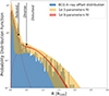 |
Fig. 4. Observed X-ray/optical miscentring distribution (blue) for the analysed total cluster sample. The plot shows the results obtained using Eq. (2). The yellow and red regions show the marginalized distribution for the 35 analysed bins without and with evolutionary terms, respectively (Eq. (3)). The red curves are the best fits for the relaxed and disturbed distribution components. |
2.5. eROSITA cluster dynamical state and BCG luminosity
To compare the BCGs luminosity as a function of the cluster’s dynamical state, we separated the DBCG − X offsets distribution into three samples. We re-defined relaxed clusters as clusters with DBCG − X < 0.25R500, disturbed clusters as clusters with DBCG − X > 0.5R500, and left everything in the middle as a diverse cluster population, as shown in Fig. 4. With this classification we find 75.4% of the sample is classified as relaxed, while 13.6% as disturbed. If, on the other side, we follow the Mann & Ebeling (2012) classification, then 28.1% are defined as relaxed, with a DBCG − X offset of less than 42 kpc, with 41 clusters with DBCG − X offset of less than 5kpc. This result is very similar when Seppi et al. (2023) criteria (DBCG − X = ΔX − O < 0.05× R500c) is used, finding a 29.1% of clusters relaxed. If we use the optical centre (DOPT − X) instead of the BCG position, as used by Seppi et al. (2023), then the number of relaxed clusters increases to 30.8%, similar to the 31% Seppi et al. (2023) found for the eFEDS sample. Ghirardini et al. (2022) also characterized the dynamical state of clusters in the eFEDS sample. They separated the sample into relaxed and disturbed clusters, using 7 X-ray morphological parameters, finding 30 to 35% of them relaxed. This is consistent with Seppi et al. (2023) and our findings.
Examples of relaxed clusters are shown in the bottom panels of Fig. 5 while examples of disturbed clusters are shown in the top panels of Fig. 5. We provide data for 15 of the most relaxed and disturbed clusters in Tables 3 and 4, respectively.
For the BCG luminosity, we obtained the griz BCG magnitudes (see Sect. 2.2) by querying BCG positions, obtained from K24, from the NOIRLab DR10 DB. We matched 95% of the sample within 1″ radius, while for the remaining 5% we used 0.5″ in the case of multiple entries and 2″ for the cases in which we find no match. For 197 BCGs, one of the bands that straddles the 4000 Å break is missing, reducing the number of clusters with colours to 3749.
To compare the BCGs brightness at different redshifts, we modelled the m* evolution and subtracted it from the cluster BCG luminosity (we used the magnitude corresponding to the band redwards of the 4000 Å break7). We modelled the m* evolution using a passively evolving composite stellar population (see e.g. Song et al. 2012; Zenteno et al. 2016; Hennig et al. 2017), with the help of EZGAL (Mancone et al. 2010). We used the Bruzual & Charlot (2003) synthesis models, with a Chabrier initial mass function (Chabrier 2003), assuming a formation redshift at z = 3 with an exponentially decaying star formation history with τ = 0.4 Gyrs. We used six distinct metallicities to match the tilt of the colour-magnitude relation at low redshifts. The metallicities correspond to the 3L*, 2L*, L*, 0.5L*, 0.4L*, and 0.3L* luminosities (we used metallicity-luminosity relation parameters from Poggianti et al. 2001). Finally, we used the m* of the Coma cluster (Iglesias-Páramo et al. 2003) to set the absolute normalization of the m* evolution.
We find all BCGs are fainter than m* − 3.2, while the average luminosity is m* − 1.64 ± 0.02, −1.73 ± 0.02, and −1.90 ± 0.01 for the disturbed, diverse, and relaxed samples, respectively. Following Z20, we explored the BCG luminosity evolution with redshift and, thanks to the large mass range in our eRASS1 subsample (1014 ≲ M500/M⊙ ≲ 1015), we included a cluster mass dimension. We separated the cluster sample by dynamical state (following Sect. 2.5) into two mass bins (separated at M500 = 1014.4 M⊙) and two redshift bins (separated at z = 0.5). The cumulative eRASS1 clusters’ BCG luminosity distributions, for the three cluster samples in four bins, are shown in Fig. 6. For the whole mass and redshift range the BCGs in relaxed clusters are brighter than in disturbed clusters and the diverse population. Similar findings have been reported in the literature for low-redshift clusters (e.g. Wen & Han 2013; Lauer et al. 2014; Wen & Han 2015).
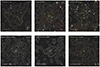 |
Fig. 5. Top: Example of three unrelaxed clusters as seen in LS composite red-green-blue images. Bottom: Example of three relaxed clusters as seen in LS composite red-green-blue images. Each image is centred at the peak of X-ray emission, shown by the red cross. White contours correspond to eROSITA X-ray contours. The cyan marker encircles the respective BCG of the cluster. The cluster redshift and cluster mass are indicated in the upper-right and lower-left corners of each panel, respectively, while the white bar shows the angular scale on the sky. North is up and east is to the left in all the images. The size of each image is 2.25R500 per side. |
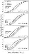 |
Fig. 6. Example of a cumulative distribution of the BCG luminosity. We used the BCG r band for z < 0.35, the i band for z < 0.7, and the z band for z > 0.7. The lines correspond to relaxed clusters (solid; DBCG − X < 0.25R500), disturbed clusters (dotted; DBCG − X > 0.5R500), and the remaining cluster sample (dashed; 0.25R500 < DBCG − X < 0.5R500). In the bottom-left corner of each panel, the number of clusters used and the KS p-value comparing the relaxed and disturbed samples are displayed. Top panel: BCGs at z ≤ 0.5 and cluster mass ≤1014.4 M⊙. Middle-top panel: BCGs at z > 0.5 and cluster mass ≤1014.4 M⊙. Middle-bottom panel: BCGs at z ≤ 0.5 and cluster mass > 1014.4 M⊙. Bottom panel: BCGs at z > 0.5 and cluster mass > 1014.4 M⊙. The shaded area corresponds to the area covered by the BCG distributions in the top panel. BCGs from the relaxed cluster sample tend to be brighter than BCGs in both the disturbed and the general population samples, most significantly at higher redshifts. |
3. Conclusions
We used the first eROSITA public data release to classify the dynamical state of 12 247 clusters and groups in order to study their DBCG − X offset distribution and its impact on the BCG luminosity. Using several quality cuts and visual inspection, we reduced the sample to 3946 clusters.
We modelled the DBCG − X offset distribution using two Rayleigh distributions, representing the relaxed and disturbed sample, as a function of redshift. From the model’s parameters (Eqs. (2) and (3)), we find that the ρ remains constant with redshift (meaning that the fraction of relaxed clusters seems to not evolve with time, which is consistent with Ghirardini et al. 2022’s findings) and mass. We find that σ0 evolves with redshift and mass, while σ1 seems to primarily evolve with mass. In other words, the offset between the BCG and the X-ray peak, in relaxed clusters, widens with redshift and for lower-mass clusters, showing how central galaxies (CGs) sink to the bottom of the potential well as the cluster grows in mass over time.
In the case of disturbed clusters, the BCGs tend to have the largest offset with their X-ray peaks in low-mass clusters, most likely due to the shallow potential well. If we use the optical centre instead of the BCG, we find similar results; Table 2 shows the same evolutionary trends for σ0 and σ1 independent of the centre used. Nevertheless, the trends are weaker when the optical centre is used. Differences could arise from the CG selection; the redMaPPer CG is determined based on more parameters (in addition to brightness and colour), including photometric redshift and the local cluster galaxy density around the CG. Selecting the CG using information about the local galaxy density may be problematic for merging clusters of similar richness (see, for example, SPT-CL J0307-6225; Hernández-Lang et al. 2022), which could dilute the signal of merging cluster rates.
To explore the impact of the dynamical state on the BCG, we separated the parent sample into relaxed (DBCG − X < 0.25R500), disturbed (DBCG − X > 0.5R500), and mixed (diverse; 0.25 < R500DBCG − X < 0.5R500) populations. We further separated the subsamples into cluster mass and cluster redshift bins. The BCG luminosity distribution can be seen in Fig. 6.
We find BCGs in relaxed clusters to be brighter than BCGs in the other two samples at all redshifts. The Kolmogorov-Smirnov (KS) p-value between the relaxed and disturbed samples is under 0.003 for all mass and redshift bins. This implies that losing access to the cluster gas affects BCG growth. This offset is most evident for the most massive clusters. Furthermore, comparing the relaxed bins to each other produces small KS p-values, while comparing the disturbed bins produces larger values. This indicates that little evolution is observed for BCGs in disturbed clusters as a function of mass and redshift, while the opposite is true for BCGs in the relaxed sample bins. This in turn indicates that the connection to the cluster gas reservoir appears to be key for BCG growth.
We used the emcee algorithm (Foreman-Mackey et al. 2013) to obtain the parameter space of the posterior distribution.
Acknowledgments
The Legacy Surveys consist of three individual and complementary projects: the Dark Energy Camera Legacy Survey (DECaLS; Proposal ID # 2014B-0404; PIs: David Schlegel and Arjun Dey), the Beijing-Arizona Sky Survey (BASS; NOAO Prop. ID #2015A-0801; PIs: Zhou Xu and Xiaohui Fan), and the Mayall z-band Legacy Survey (MzLS; Prop. ID #2016A-0453; PI: Arjun Dey). DECaLS, BASS and MzLS together include data obtained, respectively, at the Blanco telescope, Cerro Tololo Inter-American Observatory, NSF’s NOIRLab; the Bok telescope, Steward Observatory, University of Arizona; and the Mayall telescope, Kitt Peak National Observatory, NOIRLab. Pipeline processing and analyses of the data were supported by NOIRLab and the Lawrence Berkeley National Laboratory (LBNL). The Legacy Surveys project is honored to be permitted to conduct astronomical research on Iolkam Du’ag (Kitt Peak), a mountain with particular significance to the Tohono O’odham Nation. NOIRLab is operated by the Association of Universities for Research in Astronomy (AURA) under a cooperative agreement with the National Science Foundation. LBNL is managed by the Regents of the University of California under contract to the U.S. Department of Energy. This project used data obtained with the Dark Energy Camera (DECam), which was constructed by the Dark Energy Survey (DES) collaboration. Funding for the DES Projects has been provided by the US Department of Energy, the U.S. National Science Foundation, the Ministry of Science and Education of Spain, the Science and Technology Facilities Council of the United Kingdom, the Higher Education Funding Council for England, the National Center for Supercomputing Applications at the University of Illinois at Urbana-Champaign, the Kavli Institute for Cosmological Physics at the University of Chicago, Center for Cosmology and Astro-Particle Physics at the Ohio State University, the Mitchell Institute for Fundamental Physics and Astronomy at Texas A&M University, Financiadora de Estudos e Projetos, Fundação Carlos Chagas Filho de Amparo à Pesquisa do Estado do Rio de Janeiro, Conselho Nacional de Desenvolvimento Científico e Tecnológico and the Ministério da Ciência, Tecnologia e Inovação, the Deutsche Forschungsgemeinschaft and the Collaborating Institutions in the Dark Energy Survey. The Collaborating Institutions are Argonne National Laboratory, the University of California at Santa Cruz, the University of Cambridge, Centro de Investigaciones Energéticas, Medioambientales y Tecnológicas-Madrid, the University of Chicago, University College London, the DES-Brazil Consortium, the University of Edinburgh, the Eidgenössische Technische Hochschule (ETH) Zürich, Fermi National Accelerator Laboratory, the University of Illinois at Urbana-Champaign, the Institut de Ciéncies de l’Espai (IEEC/CSIC), the Institut de Física d’Altes Energies, Lawrence Berkeley National Laboratory, the Ludwig-Maximilians Universität München and the associated Excellence Cluster Universe, the University of Michigan, NSF NOIRLab, the University of Nottingham, the Ohio State University, the OzDES Membership Consortium, the University of Pennsylvania, the University of Portsmouth, SLAC National Accelerator Laboratory, Stanford University, the University of Sussex, and Texas A&M University. BASS is a key project of the Telescope Access Program (TAP), which has been funded by the National Astronomical Observatories of China, the Chinese Academy of Sciences (the Strategic Priority Research Program “The Emergence of Cosmological Structures” Grant # XDB09000000), and the Special Fund for Astronomy from the Ministry of Finance. The BASS is also supported by the External Cooperation Program of Chinese Academy of Sciences (Grant # 114A11KYSB20160057), and Chinese National Natural Science Foundation (Grant # 12120101003, # 11433005). The Legacy Survey team makes use of data products from the Near-Earth Object Wide-field Infrared Survey Explorer (NEOWISE), which is a project of the Jet Propulsion Laboratory/California Institute of Technology. NEOWISE is funded by the National Aeronautics and Space Administration. The Legacy Surveys imaging of the DESI footprint is supported by the Director, Office of Science, Office of High Energy Physics of the U.S. Department of Energy under Contract No. DE-AC02-05CH1123, by the National Energy Research Scientific Computing Center, a DOE Office of Science User Facility under the same contract; and by the U.S. National Science Foundation, Division of Astronomical Sciences under Contract No. AST-0950945 to NOAO. Based on observations made at NSF Cerro Tololo Inter-American Observatory, NSF NOIRLab (NOIRLab Prop. ID 2017A-0388; PI: A. Zenteno, ID 2018A-0386; PI: A. Zenteno, ID 2019A-0272; PI: A. Zenteno, ID 2019B-0323; PI: A. Zenteno, ID 2020A-0399; PI: A. Zenteno, ID 2020A-0909; PI: P. Arevalo, ID 2020B-0241; PI: A. Zenteno, ID 2021A-0149; PI: A. Zenteno, ID 2021A-0922; PI: J. L. Nilo-Castellón, 2022A-597406; PI: A. Zenteno), which is managed by the Association of Universities for Research in Astronomy (AURA) under a cooperative agreement with the U.S. National Science Foundation. This work is based on data from eROSITA, the soft X-ray instrument aboard SRG, a joint Russian-German science mission supported by the Russian Space Agency (Roskosmos), in the interests of the Russian Academy of Sciences represented by its Space Research Institute (IKI), and the Deutsches Zentrum für Luft und Raumfahrt (DLR). The SRG spacecraft was built by Lavochkin Association (NPOL) and its subcontractors and is operated by NPOL with support from the Max Planck Institute for Extraterrestrial Physics (MPE). The development and construction of the eROSITA X-ray instrument were led by MPE, with contributions from the Dr. Karl Remeis Observatory Bamberg & ECAP (FAU Erlangen-Nuernberg), the University of Hamburg Observatory, the Leibniz Institute for Astrophysics Potsdam (AIP), and the Institute for Astronomy and Astrophysics of the University of Tübingen, with the support of DLR and the Max Planck Society. The Argelander Institute for Astronomy of the University of Bonn and the Ludwig Maximilians Universität Munich also participated in the science preparation for eROSITA. E. Bulbul, A. Liu, V. Ghirardini, X. Zhang acknowledge financial support from the European Research Council (ERC) Consolidator Grant under the European Union’s Horizon 2020 research and innovation program (grant agreement CoG DarkQuest No 101002585). German eROSITA consortium.
References
- Abbott, T. M. C., Abdalla, F. B., Allam, S., et al. 2018, ApJS, 239, 18 [Google Scholar]
- Abriola, D., Della Pergola, D., Lombardi, M., et al. 2024, A&A, 684, A193 [NASA ADS] [CrossRef] [EDP Sciences] [Google Scholar]
- Akamatsu, H., Takizawa, M., Nakazawa, K., et al. 2012, PASJ, 64, 67 [NASA ADS] [Google Scholar]
- Albuquerque, R. P., Machado, R. E. G., & Monteiro-Oliveira, R. 2024, MNRAS, 530, 2146 [Google Scholar]
- Aldás, F., Zenteno, A., Gómez, F. A., et al. 2023, MNRAS, 525, 1769 [CrossRef] [Google Scholar]
- Artis, E., Ghirardini, V., Bulbul, E., et al. 2024, The SRG-eROSITA All-Sky Survey : Constraints on f(R) Gravity from Cluster Abundance [Google Scholar]
- Bahar, Y. E., Bulbul, E., Clerc, N., et al. 2022, A&A, 661, A7 [NASA ADS] [CrossRef] [EDP Sciences] [Google Scholar]
- Balzer, F., Bulbul, E., Kluge, M., et al. 2025, A&A, submitted [arXiv:2501.17238] [Google Scholar]
- Bleem, L. E., Stalder, B., de Haan, T., et al. 2015, ApJS, 216, 27 [Google Scholar]
- Bocquet, S., & Carter, F. W. 2016, J. Open Source Software, 1, 46 [NASA ADS] [CrossRef] [Google Scholar]
- Bocquet, S., Saro, A., Mohr, J. J., et al. 2015, ApJ, 799, 214 [NASA ADS] [CrossRef] [Google Scholar]
- Bocquet, S., Grandis, S., Bleem, L. E., et al. 2024, Phys. Rev. D, 110, 083510 [NASA ADS] [CrossRef] [Google Scholar]
- Botteon, A., Cassano, R., Eckert, D., et al. 2019, A&A, 630, A77 [NASA ADS] [CrossRef] [EDP Sciences] [Google Scholar]
- Brouwer, M. M., Oman, K. A., Valentijn, E. A., et al. 2021, A&A, 650, A113 [NASA ADS] [CrossRef] [EDP Sciences] [Google Scholar]
- Bruzual, G., & Charlot, S. 2003, MNRAS, 344, 1000 [NASA ADS] [CrossRef] [Google Scholar]
- Bulbul, E., Markevitch, M., Foster, A., et al. 2014, ApJ, 789, 13 [NASA ADS] [CrossRef] [Google Scholar]
- Bulbul, E., Liu, A., Kluge, M., et al. 2024, A&A, 685, A106 [NASA ADS] [CrossRef] [EDP Sciences] [Google Scholar]
- Capalbo, V., De Petris, M., De Luca, F., et al. 2021, MNRAS, 503, 6155 [Google Scholar]
- Chabrier, G. 2003, PASP, 115, 763 [Google Scholar]
- Chan, M. H., & Del Popolo, A. 2020, MNRAS, 492, 5865 [NASA ADS] [CrossRef] [Google Scholar]
- Chiu, I. N., Klein, M., Mohr, J., & Bocquet, S. 2023, MNRAS, 522, 1601 [NASA ADS] [CrossRef] [Google Scholar]
- Costanzi, M., Saro, A., Bocquet, S., et al. 2021, Phys. Rev. D, 103, 043522 [Google Scholar]
- Cui, W., Power, C., Borgani, S., et al. 2017, MNRAS, 464, 2502 [NASA ADS] [CrossRef] [Google Scholar]
- De Luca, F., De Petris, M., Yepes, G., et al. 2021, MNRAS, 504, 5383 [NASA ADS] [CrossRef] [Google Scholar]
- Dey, A., Schlegel, D. J., Lang, D., et al. 2019, AJ, 157, 168 [Google Scholar]
- Doubrawa, L., Machado, R. E. G., Laganá, T. F., et al. 2020, MNRAS, 495, 2022 [Google Scholar]
- Doubrawa, L., Cypriano, E. S., Finoguenov, A., et al. 2023, MNRAS, 526, 4285 [NASA ADS] [CrossRef] [Google Scholar]
- Dressler, A. 1980, ApJ, 236, 351 [Google Scholar]
- Drlica-Wagner, A., Carlin, J. L., Nidever, D. L., et al. 2021, ApJS, 256, 2 [NASA ADS] [CrossRef] [Google Scholar]
- Drlica-Wagner, A., Ferguson, P. S., Adamów, M., et al. 2022, ApJS, 261, 38 [NASA ADS] [CrossRef] [Google Scholar]
- Duffy, A. R., Schaye, J., Kay, S. T., & Dalla Vecchia, C. 2008, MNRAS, 390, L64 [Google Scholar]
- Fischer, M. S., Durke, N.-H., Hollingshausen, K., et al. 2023, MNRAS, 523, 5915 [CrossRef] [Google Scholar]
- Flaugher, B., Diehl, H. T., Honscheid, K., et al. 2015, AJ, 150, 150 [Google Scholar]
- Foreman-Mackey, D., Hogg, D. W., Lang, D., & Goodman, J. 2013, PASP, 125, 306 [Google Scholar]
- Fumagalli, A., Costanzi, M., Saro, A., Castro, T., & Borgani, S. 2024, A&A, 682, A148 [NASA ADS] [CrossRef] [EDP Sciences] [Google Scholar]
- Gaia Collaboration (Prusti, T., et al.) 2016, A&A, 595, A1 [NASA ADS] [CrossRef] [EDP Sciences] [Google Scholar]
- Ghirardini, V., Bahar, Y. E., Bulbul, E., et al. 2022, A&A, 661, A12 [NASA ADS] [CrossRef] [EDP Sciences] [Google Scholar]
- Ghirardini, V., Bulbul, E., Artis, E., et al. 2024, A&A, 689, A298 [NASA ADS] [CrossRef] [EDP Sciences] [Google Scholar]
- Harvey, D., Massey, R., Kitching, T., Taylor, A., & Tittley, E. 2015, Science, 347, 1462 [Google Scholar]
- Hennig, C., Mohr, J. J., Zenteno, A., et al. 2017, MNRAS, 467, 4015 [NASA ADS] [Google Scholar]
- Hernández-Lang, D., Zenteno, A., Diaz-Ocampo, A., et al. 2022, MNRAS, 517, 4355 [Google Scholar]
- Hlavacek-Larrondo, J., Li, Y., & Churazov, E. 2022, in Handbook of X-ray and Gamma-ray Astrophysics, 5 [Google Scholar]
- Ider Chitham, J., Comparat, J., Finoguenov, A., et al. 2020, MNRAS, 499, 4768 [NASA ADS] [CrossRef] [Google Scholar]
- Iglesias-Páramo, J., Boselli, A., Gavazzi, G., Cortese, L., & Vílchez, J. M. 2003, A&A, 397, 421 [NASA ADS] [CrossRef] [EDP Sciences] [Google Scholar]
- Kelkar, K., Dwarakanath, K. S., Poggianti, B. M., et al. 2020, MNRAS, 496, 442 [NASA ADS] [CrossRef] [Google Scholar]
- Klein, M., Mohr, J. J., Desai, S., et al. 2017, MNRAS, 474, 3324 [Google Scholar]
- Klein, M., Grandis, S., Mohr, J. J., et al. 2019, MNRAS, 488, 739 [Google Scholar]
- Kluge, M., Comparat, J., Liu, A., et al. 2024, A&A, 688, A210 [NASA ADS] [CrossRef] [EDP Sciences] [Google Scholar]
- Lang, D., Hogg, D. W., & Mykytyn, D. 2016, The Tractor: Probabilistic astronomical source detection and measurement, Astrophysics Source Code Library [record ascl:1604.008] [Google Scholar]
- Lauer, T. R., Postman, M., Strauss, M. A., Graves, G. J., & Chisari, N. E. 2014, ApJ, 797, 82 [Google Scholar]
- Lindegren, L., Hernández, J., Bombrun, A., et al. 2018, A&A, 616, A2 [NASA ADS] [CrossRef] [EDP Sciences] [Google Scholar]
- Liu, A., Bulbul, E., Ghirardini, V., et al. 2022, A&A, 661, A2 [NASA ADS] [CrossRef] [EDP Sciences] [Google Scholar]
- Lopes, P. A. A., Trevisan, M., Laganá, T. F., et al. 2018, MNRAS, 478, 5473 [Google Scholar]
- Lourenço, A. C. C., Lopes, P. A. A., Laganá, T. F., et al. 2020, MNRAS, 498, 835 [CrossRef] [Google Scholar]
- Lourenço, A. C. C., Jaffé, Y. L., Vulcani, B., et al. 2023, MNRAS, 526, 4831 [CrossRef] [Google Scholar]
- Lovisari, L., & Maughan, B. J. 2022, in Handbook of X-ray and Gamma-ray Astrophysics, 65 [Google Scholar]
- Machado, R. E. G., & Lima Neto, G. B. 2013, MNRAS, 430, 3249 [NASA ADS] [CrossRef] [Google Scholar]
- Machado, R. E. G., Monteiro-Oliveira, R., Lima Neto, G. B., & Cypriano, E. S. 2015, MNRAS, 451, 3309 [NASA ADS] [CrossRef] [Google Scholar]
- Mancone, C. L., Gonzalez, A. H., Brodwin, M., et al. 2010, ApJ, 720, 284 [NASA ADS] [CrossRef] [Google Scholar]
- Mann, A. W., & Ebeling, H. 2012, MNRAS, 420, 2120 [NASA ADS] [CrossRef] [Google Scholar]
- Markevitch, M., & Vikhlinin, A. 2007, Phys. Rep., 443, 1 [Google Scholar]
- Merloni, A., Predehl, P., Becker, W., et al. 2012, arXiv e-prints [arXiv:1209.3114] [Google Scholar]
- Merloni, A., Lamer, G., Liu, T., et al. 2024, A&A, 682, A34 [NASA ADS] [CrossRef] [EDP Sciences] [Google Scholar]
- Molnar, S. 2016, Front. Astron. Space Sci., 2, 7 [NASA ADS] [CrossRef] [Google Scholar]
- Monteiro-Oliveira, R. 2022, MNRAS, 515, 3674 [CrossRef] [Google Scholar]
- Monteiro-Oliveira, R., Lima Neto, G. B., Cypriano, E. S., et al. 2017, MNRAS, 468, 4566 [NASA ADS] [CrossRef] [Google Scholar]
- Monteiro-Oliveira, R., Soja, A. C., Ribeiro, A. L. B., et al. 2021, MNRAS, 501, 756 [Google Scholar]
- Monteiro-Oliveira, R., Morell, D. F., Sampaio, V. M., Ribeiro, A. L. B., & de Carvalho, R. R. 2022, MNRAS, 509, 3470 [Google Scholar]
- Moura, M. T., Machado, R. E. G., & Monteiro-Oliveira, R. 2021, MNRAS, 500, 1858 [Google Scholar]
- Neilsen, H., Bernstein, G., Gruendl, R., & Kent, S. 2016 [Google Scholar]
- Nelson, D., Pillepich, A., Ayromlou, M., et al. 2024, A&A, 686, A157 [NASA ADS] [CrossRef] [EDP Sciences] [Google Scholar]
- Pandge, M. B., Monteiro-Oliveira, R., Bagchi, J., et al. 2019, MNRAS, 482, 5093 [NASA ADS] [CrossRef] [Google Scholar]
- Peng, Y.-J., Lilly, S. J., Kovač, K., et al. 2010, ApJ, 721, 193 [Google Scholar]
- Poggianti, B. M., Bridges, T. J., Mobasher, B., et al. 2001, ApJ, 562, 689 [NASA ADS] [CrossRef] [Google Scholar]
- Predehl, P., Andritschke, R., Arefiev, V., et al. 2021, A&A, 647, A1 [EDP Sciences] [Google Scholar]
- Ruggiero, R., Machado, R. E. G., Roman-Oliveira, F. V., et al. 2019, MNRAS, 484, 906 [Google Scholar]
- Ruszkowski, M., & Pfrommer, C. 2023, A&A Rev., 31, 4 [NASA ADS] [CrossRef] [Google Scholar]
- Rykoff, E. S., Koester, B. P., Rozo, E., et al. 2012, ApJ, 746, 178 [NASA ADS] [CrossRef] [Google Scholar]
- Rykoff, E. S., Rozo, E., Busha, M. T., et al. 2014, ApJ, 785, 104 [Google Scholar]
- Rykoff, E. S., Rozo, E., Hollowood, D., et al. 2016, ApJS, 224, 1 [NASA ADS] [CrossRef] [Google Scholar]
- Sarazin, C. L. 2004, J. Korean Astron. Soc., 37, 433 [Google Scholar]
- Saro, A., Bocquet, S., Rozo, E., et al. 2015, MNRAS, 454, 2305 [Google Scholar]
- Seppi, R., Comparat, J., Nandra, K., et al. 2023, A&A, 671, A57 [NASA ADS] [CrossRef] [EDP Sciences] [Google Scholar]
- Sirks, E. L., Harvey, D., Massey, R., et al. 2024, MNRAS, 530, 3160 [Google Scholar]
- Soja, A. C., Sodré, L., Monteiro-Oliveira, R., Cypriano, E. S., & Lima Neto, G. B. 2018, MNRAS, 477, 3279 [Google Scholar]
- Song, J., Zenteno, A., Stalder, B., et al. 2012, ApJ, 761, 22 [NASA ADS] [CrossRef] [Google Scholar]
- Tam, S.-I., Umetsu, K., Robertson, A., & McCarthy, I. G. 2023, ApJ, 953, 169 [CrossRef] [Google Scholar]
- Ueda, S., Ichinohe, Y., Molnar, S. M., Umetsu, K., & Kitayama, T. 2020, ApJ, 892, 100 [NASA ADS] [CrossRef] [Google Scholar]
- Ueda, S., Umetsu, K., Ng, F., et al. 2021, ApJ, 922, 81 [Google Scholar]
- Valdes, F., Gruendl, R., & DES Project, 2014, in Astronomical Data Analysis Software and Systems XXIII, eds. N. Manset, & P. Forshay, ASP Conf. Ser., 485, 379. [Google Scholar]
- Véliz Astudillo, S., Carrasco, E. R., Nilo Castellón, J. L., Zenteno, A., & Cuevas, H. 2025, A&A, 693, A106 [NASA ADS] [CrossRef] [EDP Sciences] [Google Scholar]
- Wen, Z. L., & Han, J. L. 2013, MNRAS, 436, 275 [Google Scholar]
- Wen, Z. L., & Han, J. L. 2015, MNRAS, 448, 2 [Google Scholar]
- Wittman, D., Imani, D., Olden, R. H., & Golovich, N. 2024, AJ, 167, 49 [Google Scholar]
- Yoon, M., Lee, W., Jee, M. J., et al. 2020, ApJ, 903, 151 [CrossRef] [Google Scholar]
- Yuan, Z. S., & Han, J. L. 2020, MNRAS, 497, 5485 [Google Scholar]
- Yuan, Z. S., Han, J. L., & Wen, Z. L. 2022, MNRAS, 513, 3013 [NASA ADS] [CrossRef] [Google Scholar]
- Zenteno, A., Mohr, J. J., Desai, S., et al. 2016, MNRAS, 462, 830 [NASA ADS] [CrossRef] [Google Scholar]
- Zenteno, A., Hernández-Lang, D., Klein, M., et al. 2020, MNRAS, 495, 705 [Google Scholar]
- ZuHone, J. A. 2011, ApJ, 728, 54 [Google Scholar]
All Tables
All Figures
|
Fig. 1. Best-fit ρ, σ0, and σ1 parameters in bins of mass and redshift derived from Eq. (2). For σ, trends with both redshift and mass are observed. |
| In the text | |
|
Fig. 2. Marginalized distribution for ρ, σ0, and σ1 as a function of the mean redshift and mean mass of each analysed bin derived with Eq. (2). The fraction of (un)relaxed clusters (1 − ρ) ρ remains constant across redshifts, while we find a positive correlation of σ0 with redshift and a negative correlation of σ1 with mass. |
| In the text | |
|
Fig. 3. Marginalized distribution of the miscentring model described by Eqs. (2) and (3). σ0 has a positive correlation with redshift ( |
| In the text | |
|
Fig. 4. Observed X-ray/optical miscentring distribution (blue) for the analysed total cluster sample. The plot shows the results obtained using Eq. (2). The yellow and red regions show the marginalized distribution for the 35 analysed bins without and with evolutionary terms, respectively (Eq. (3)). The red curves are the best fits for the relaxed and disturbed distribution components. |
| In the text | |
|
Fig. 5. Top: Example of three unrelaxed clusters as seen in LS composite red-green-blue images. Bottom: Example of three relaxed clusters as seen in LS composite red-green-blue images. Each image is centred at the peak of X-ray emission, shown by the red cross. White contours correspond to eROSITA X-ray contours. The cyan marker encircles the respective BCG of the cluster. The cluster redshift and cluster mass are indicated in the upper-right and lower-left corners of each panel, respectively, while the white bar shows the angular scale on the sky. North is up and east is to the left in all the images. The size of each image is 2.25R500 per side. |
| In the text | |
|
Fig. 6. Example of a cumulative distribution of the BCG luminosity. We used the BCG r band for z < 0.35, the i band for z < 0.7, and the z band for z > 0.7. The lines correspond to relaxed clusters (solid; DBCG − X < 0.25R500), disturbed clusters (dotted; DBCG − X > 0.5R500), and the remaining cluster sample (dashed; 0.25R500 < DBCG − X < 0.5R500). In the bottom-left corner of each panel, the number of clusters used and the KS p-value comparing the relaxed and disturbed samples are displayed. Top panel: BCGs at z ≤ 0.5 and cluster mass ≤1014.4 M⊙. Middle-top panel: BCGs at z > 0.5 and cluster mass ≤1014.4 M⊙. Middle-bottom panel: BCGs at z ≤ 0.5 and cluster mass > 1014.4 M⊙. Bottom panel: BCGs at z > 0.5 and cluster mass > 1014.4 M⊙. The shaded area corresponds to the area covered by the BCG distributions in the top panel. BCGs from the relaxed cluster sample tend to be brighter than BCGs in both the disturbed and the general population samples, most significantly at higher redshifts. |
| In the text | |
Current usage metrics show cumulative count of Article Views (full-text article views including HTML views, PDF and ePub downloads, according to the available data) and Abstracts Views on Vision4Press platform.
Data correspond to usage on the plateform after 2015. The current usage metrics is available 48-96 hours after online publication and is updated daily on week days.
Initial download of the metrics may take a while.