| Issue |
A&A
Volume 693, January 2025
|
|
|---|---|---|
| Article Number | A9 | |
| Number of page(s) | 19 | |
| Section | Extragalactic astronomy | |
| DOI | https://doi.org/10.1051/0004-6361/202449636 | |
| Published online | 23 December 2024 | |
Kilogauss magnetic field and jet dynamics in the quasar NRAO 530
1
Instituto de Física, Pontificia Universidad Católica de Valparaíso, Casilla, 4059 Valparaíso, Chile
2
Max-Planck-Institut für Radioastronomie, Auf dem Hügel 69, D-53121 Bonn, Germany
3
Astro Space Center, Lebedev Physical Institute, Profsouznaya 84/32, Moscow 117997, Russia
4
Institute for Astrophysical Research, Boston University, 725 Commonwealth Ave., Boston, MA 02215, USA
5
Saint Petersburg State University, Universitetskaya Nab. 7-9, St. Petersburg 199034, Russia
6
Instituto de Astrofísica de Andalucía-CSIC, Glorieta de la Astronomía s/n, E-18008 Granada, Spain
7
Moscow Institute of Physics and Technology, Institutsky Per. 9, Moscow Region, Dolgoprudny 141700, Russia
8
Korea Astronomy and Space Science Institute, Daedeok-daero 776, Yuseong-gu, Daejeon 34055, Republic of Korea
9
Department of Astronomy, Yonsei University, Yonsei-ro 50, Seodaemun-gu, Seoul 03722, Republic of Korea
10
Center for Astrophysics | Harvard & Smithsonian, 60 Garden Street, Cambridge, MA 02138, USA
11
Department of Physics, Faculty of Science, University of Malaya, 50603 Kuala Lumpur, Malaysia
12
IRAM (Instituto de Radioastronomía Milimétrica), Avda. Divina Pastora 7, Local 20, 18012 Granada, Spain
⋆ Corresponding author; mikhail@lisakov.com
Received:
16
February
2024
Accepted:
30
October
2024
Context. The advancement of the Event Horizon Telescope has enabled the study of relativistic jets in active galactic nuclei down to sub-parsec linear scales even at high redshift. Quasi-simultaneous multifrequency observations provide insights into the physical conditions in compact regions and allow accretion theories to be tested.
Aims. Initially, we aimed to measure the magnetic field strength close to the central supermassive black hole in NRAO 530 (1730−130) by studying the frequency-dependent opacity of the jet matter, Faraday rotation, and the spectral index in the millimeter-radio bands.
Methods. NRAO 530 was observed quasi-simultaneously at 15, 22, 43, 86, and 227 GHz at four different very long baseline interferometer (VLBI) networks. By means of imaging and model-fitting, we aligned the images, taken at different frequencies. We explored opacity along the jet and the distribution of the linearly polarized emission in it.
Results. Our findings reveal that the jet of NRAO 530 at 86 and 227 GHz is transparent down to its origin, with 70 mJy emission detected at 227 GHz potentially originating from the accretion disk. The magnetic field strength near the black hole, estimated at 5rg, is 3 × 10³ − 3 × 10⁴ G (depending on the central black hole mass). These values represent some of the highest magnetic field strengths reported for active galaxies. We also report the first ever VLBI measurement of the Faraday rotation at 43−227 GHz, which reveals rotation measure values as high as −48 000 rad/m2, consistent with higher particle density and stronger magnetic fields at the jet’s outset. The complex shape of the jet in NRAO 530 is in line with the expected behavior of a precessing jet, with a period estimated to be around 6 ± 4 years.
Key words: accretion / accretion disks / techniques: interferometric / galaxies: jets / galaxies: magnetic fields / quasars: supermassive black holes / quasars: individual: NRAO 530
© The Authors 2024
 Open Access article, published by EDP Sciences, under the terms of the Creative Commons Attribution License (https://creativecommons.org/licenses/by/4.0), which permits unrestricted use, distribution, and reproduction in any medium, provided the original work is properly cited.
This article is published in open access under the Subscribe to Open model. Subscribe to A&A to support open access publication.
1. Introduction
The quasar NRAO 530 (1730−130, J1733−1304) is a radio-loud compact source that belongs to the sub-class of blazars, which exhibit highly variable nonthermal emission. It possesses a highly relativistic jet with an apparent speed exceeding 30c (Weaver et al. 2022), bright γ-ray emission (Abdollahi et al. 2020), and prominent variability of the optical linear polarization1. On parsec scales, the jet is directed to the north (e.g., Lister et al. 2019), while the kilo-parsec scale jet is perpendicular to this direction, extending from east to west over 3″ (Kharb et al. 2010). Although quasars are generally associated with the Fanaroff-Riley II (FRII) type of extragalactic radio sources, the NRAO 530 kilo-parsec scale jet has a hybrid morphology, with a diffuse eastern portion displaying FRI-type features, but compact emission on the western side agrees better with the FRII properties. This complex structure of the jet can be explored by multifrequency radio observations. Such a probe of the properties of the radio jet was presented in Lu (2010) using quasi-simultaneous observations obtained in 2007 at 86, 43, 22 GHz, and 15 GHz. That author identified the southernmost component of the jet as the apparent “core” based on its flat spectral index, while components farther down the jet have optically thin spectral indices that evolve with distance from the core in a quasi-sinusoidal pattern with an increasing characteristic scale. The data also indicate a frequency-dependent core shift not only along the jet but also transverse to the jet. Hovatta et al. (2012, 2014) have analyzed the spectral characteristics and Faraday rotation measure (RM) in the parsec-scale jet of NRAO 530 at four lower frequencies between 8.1 and 15.4 GHz within the MOJAVE (Monitoring of Jets in Active Galactic Nuclei with VLBA Experiments) sample. They have also found a flat spectral index of the core (α = −0.10, Sν ∝ να) and a steep spectral index of the extended jet (α = −1.14), as well as relatively low values of RM both around the core region (371 rad m−2) and in the jet (0.9 rad m−2). An et al. (2013) investigated periodicity in the radio light curves of NRAO 530 at 14.5, 8, and 4.5 GHz using UMRAO (University of Michigan Radio Astronomy Observatory) data (Aller et al. 1985) from 1967 to 2012. They detected two strong and persistent periods of ∼10 yr and ∼6 yr and several weaker shorter-timescale periodicities of ∼3.5, ∼3, and ∼2 yr. The authors found that the characteristic frequencies of these periodicities have a harmonic relationship. An et al. (2013) suggested that the multiplicity and apparent harmonic relation of the periodicity can be interpreted by the global p-mode oscillation of the accretion disk, implying a disk-jet connection. However, it can be explained also by magnetohydrodynamic (MHD) instabilities (Istomin & Pariev 1996; Narayan et al. 2009; Mizuno et al. 2012) or Lense–Thirring precession (Thirring 1918) observed by Britzen et al. (2023), von Fellenberg et al. (2023), Cui et al. (2023).
Owing to its brightness, compact nature, and position on the sky, NRAO 530 is often used as a calibrator for Very Long Baseline Interferometric (VLBI) observations of the radio source Sagittarius A* (Sgr A*) located at the center of our Galaxy (e.g., Lu et al. 2011). This was also the case for the Event Horizon Telescope (EHT) observations of Sgr A* in April 2017 (EHT Collaboration 2022a). Jorstad et al. (2023) have presented total and polarized intensity images of NRAO 530 obtained during the EHT campaign at 227 GHz. The source has a multicomponent structure extended to the northwest, with linear polarization detected in the core and jet. For the purpose of this research, we have collected VLBI data of the quasar at 86, 43, 22, and 15 GHz contemporaneous to the EHT observation. With an EHT resolution of ∼20 micro-arcseconds (μas) and the extension of the jet at 15 GHz out to 25 mas from the core, the combined dataset covers a wide range of spatial scales, from sub-parsec (∼0.15 pc) to ∼200 pc projected distances, based on the quasar redshift of z = 0.902 (Junkkarinen 1984). This corresponds to the linear scale of 7.9 pc mas−1 with the cosmological parameters H0 = 67.7 km s−1 Mpc−1, ΩM = 0.307, and ΩΛ = 0.693 (Wright 2006; Planck Collaboration XIII 2016). In accord with Jorstad et al. (2023), we adopted the following parameters for the source: Doppler factor at mas-scales of δ = 9, a viewing angle of α = 3°, and a bulk Lorentz factor of Γ = 8 (Weaver et al. 2022).
The multifrequency VLBI data allow us to study the structure, spectral characteristics, and polarization properties of the jet of NRAO 530 on multiple scales, from the vicinity of the black hole (BH) to hundreds of parsecs down the jet. The outline of the paper is as follows: data sources, their issues, and data reduction methods are discussed in Sect. 2; the magnetic field is estimated in Sect. 3; the spatial structure of NRAO 530 at multiple frequencies is covered in Sect. 4; the brightness temperature is discussed in Sect. 5; source structure in linear polarization and Faraday RM are presented in Sect. 6; and, finally, a coherent model of the source is discussed in Sect. 7.
2. Data and methods
2.1. 227 GHz
NRAO 530 was observed by the EHT on April 5−7, 2017, as a calibrator of Sagittarius A* (EHT Collaboration 2022a,b). The source was observed with the full EHT array composed of eight stations at six geographical sites: the Atacama Large Millimeter/submillimeter Array (ALMA, operating as a phased array; Goddi et al. 2019) and the Atacama Pathfinder Experiment (APEX) telescope in Chile; the Large Millimeter Telescope Alfonso Serrano (LMT) in Mexico; the IRAM (Instituto de Radioastronomía Milimétrica) 30 m telescope (PV) in Spain; the Submillimeter Telescope (SMT) in Arizona; the James Clerk Maxwell Telescope (JCMT) and the Submillimeter Array (SMA) in Hawai’i; and the South Pole Telescope (SPT) in Antarctica. Two 2 GHz-wide frequency bands, centered at 227.1 GHz and 229.1 GHz, were recorded with full polarization, with the exception of a single-polarization JCMT. Subsequent data reduction, calibration, and validation were described in Blackburn et al. (2019), Janssen et al. (2019), EHT Collaboration (2019), with minor updates of the data reduction pipeline described in EHT Collaboration (2022b), and the detailed polarimetric leakage calibration follows EHT Collaboration (2021a) and Issaoun et al. (2022). The absolute calibration of the electric vector position angle (EVPA) follows the highly accurate polarimetric calibration of ALMA (Goddi et al. 2019; EHT Collaboration 2021a). A detailed analysis of the NRAO 530 EHT dataset and resulting total intensity and linear polarization images was performed by Jorstad et al. (2023). In this study, we have used the fiducial total and polarized intensity images presented in Jorstad et al. (2023), which were obtained by combining data over all days and both frequencies, since no unambiguous temporal of spectral variability has been detected during the 3 consecutive days of the EHT observations.
2.2. 86 GHz
The source was observed with the Global Millimeter VLBI Array (GMVA), consisting of the eight Very Long Baseline Array (VLBA) stations equipped with 86 GHz receivers, the Green Bank Telescope (GB), the Yebes 40-m telescope (YS), the IRAM 30-m telescope (PV), the Effelsberg 100-m telescope (EB), and the ALMA phased array. The observations were conducted on April 3, 2017, over 7.5 h, as a part of a Sgr A* observing campaign (GMVA project MB007), for which NRAO 530 served as a calibrator (Issaoun et al. 2019). The data were recorded at four intermediate-frequency bands (IFs) centered at 86.06, 86.12, 86.18, and 86.24 GHz, with a total bandwidth of 256 MHz per polarization. Corresponding total intensity images of NRAO 530, obtained through the closure-only imaging method (Chael et al. 2018), were published by Issaoun et al. (2019). For consistency with other images obtained at low frequencies (see below), we have performed both total and polarized intensity imaging of the 86 GHz data using the traditional VLBI CLEAN method implemented in the DIFMAP (Shepherd 1997) software package, with the approach to high-frequency VLBI data described in Casadio et al. (2019). Due to uncertain amplitude calibration of some GMVA stations in this observation, the total VLBI-flux at 86 GHz was scaled to 2.74 Jy, measured by ALMA on April 3, 2017 (Goddi et al. 2019). The data were corrected for the polarimetric leakage D-terms following the prescription defined in Leppänen et al. (1995) using the LPCAL task in the Astronomical Imaging Processing System (AIPS) supplied by the National Radio Astronomy Observatory (NRAO). We performed several analyses to search for D-terms: (1) using NRAO 530 for determining D-terms for each IF; (2) using NRAO 530 with data combined over all IFs; and (3) averaging D-term solutions derived for NRAO 530 and OJ 287 observed in the same run (Zhao et al. 2022) with data combined over all IFs. We have found that the lowest level of the noise (rms) for Stokes Q and U maps is achieved in the case of data corrected with D-terms obtained for the NRAO 530 solutions with data combined over IFs. The EVPA calibration was obtained by comparing the polarization position angle integrated over the NRAO 530 image with the one measured by ALMA (Goddi et al. 2019), which provides an EVPA measurement accuracy of ±6°.
2.3. 43 GHz
The dataset at 43 GHz (λ = 7 mm) was obtained as part of the VLBA-BU-BLAZAR program2, which includes monthly observations of a sample of 38 radio and γ-ray bright active galactic nuclei (AGNs) over 24 h at each epoch. The data and calibration details description are given in Jorstad et al. (2017). NRAO 530 was observed on March 19 and April 16, 2017, with a 50 and 45 min integration time per source (9 and 10 scans of 5-min duration), respectively, at a recording rate of 2048 Mb per second (Mbps). Observations were performed in full polarization mode in the 256 MHz bandwidth, which is split into four IFs centered at 43.0075, 43.0875, 43.1515, and 43.2155 GHz. A final set of D-terms used at each epoch was obtained by averaging solutions over 15 sources in the sample for which there was the best agreement between the D-terms. The EVPA calibration was obtained by different methods: a comparison of the Very Large Array (VLA) and VLBA integrated EVPAs at quasi-simultaneous epochs, the D-term method (Gómez 2002), and using EVPA-stable features (for a period of several months) in the images of the jets of 3C 279, OJ 287, 3C 446, and 3C 454.3, which allowed us to reach an accuracy of ±5°.
2.4. 22 GHz
The 22 GHz (λ = 1.3 cm) data were obtained from the East Asian VLBI Network (EAVN), which consists of the KaVA (KVN3 and VERA4 Array; e.g., Niinuma et al. 2015; Hada et al. 2017; Park et al. 2019) and additional East Asian telescopes (e.g., Tianma-65m, Nanshan-26m, and Hitachi-32m telescopes; Cui et al. 2021). In this study, we have analyzed the EAVN observation from April 3, which is part of the KaVA/EAVN Large Program toward Sgr A* (Cho et al. 2022). The NRAO 530 has been observed as one of the calibrators with an on-source time of ∼30 minutes. The data were recorded with a total bandwidth of 256 MHz (32 MHz × 8 channels) and single RCP polarization. A total of ten telescopes have participated (seven telescopes of KaVA, Tianma-65m, Nanshan-26m, and Hitachi-32m), but the Nanshan-26m and Hitachi-32m were withdrawn due to a severe problem with their antenna gains.
2.5. 15 GHz
NRAO 530 is included in the regular monitoring of the 2 cm VLBA survey (Kellermann et al. 1998), which nowadays is followed by the MOJAVE5 program (Lister et al. 2021). The closest observations to the 2017 EHT session were performed on January 3 and May 25. The data were taken in the dual polarization mode at a central frequency of 15.369 GHz. The data were recorded at 2048 Mbps with 2-bit sampling in a bandwidth of 256 MHz per polarization. The EVPA and flux density accuracy are estimated to be ∼5° and ∼5%, respectively (Lister et al. 2018).
2.6. Modeling and cross-frequency alignment of images
The first essential step that allows us to extract physical information from the images and UV data is fitting the structure of the jet with a small number of 2D Gaussians, hereafter named components. This fitting was performed in the UV domain using the MODELFIT procedure in DIFMAP. The parameters of all of the model components are listed in Table C.1. Optically thin components at different frequencies were used to determine the shift between images at these frequencies, a crucial step for all subsequent analysis. This step is required since the information about the absolute coordinates of the source is lost during the data reduction and imaging processes.
To obtain the most accurate image alignment, we performed it in two steps. First, for each pair of adjacent frequencies, we fit the models using only a common range of UV distances in order to equalize resolution. This was possible for all frequency pairs except for 86−227 GHz, which have only 5% of their visibilities in the common UV range. This approach allowed us to get a similar structure of the jet at both frequencies in the pair and provided a robust estimate of the alignment shift between the maps. For most of the frequency pairs, there were several pairs of cross-identified components. The final shift was calculated as an average of all pairs of cross-identified components weighted with the ratio of their flux density and size, as follows:
where Riνx is the component’s position at frequency νx. The weights were calculated as
where Fiνx and Siνx are the component’s flux density and size at frequency νx. Normalizing weights to the average at a given frequency accounts for different angular resolution and total flux at different frequencies. With this approach, the brightest and the most compact components contributed most to the derived shift. Since we have used distinct, bright, and compact components for this analysis, the uncertainty of the derived shift is less than 10 μas in all cases. Examples of the alignment are collected in Appendix A.
Second, at each frequency, we fit the best model to the data using the full available range of UV distances. At all frequencies, these MODELFIT models are of comparable quality to the CLEAN models. The shifts derived in the first step were used to align these models and reveal the multifrequency structure of the jet, as is presented in Fig. 1.
 |
Fig. 1. 2D Gaussian best-fit models of NRAO 530 at five frequencies, after alignment. Each resolved Gaussian component is shown as a circle with a diameter of the FWHM of the component. Unresolved components are shown as crosses. Different colors correspond to different frequencies in the dataset, as is shown in the legend. Gray contours represent the source structure at 43 GHz convolved with a circular beam. Horizontal arrows indicate the position of the apparent jet beginning at 227 and 86 GHz, 43 GHz, and 15 and 22 GHz (bottom to top). |
Since 15 and 43 GHz observations were not coordinated with the EHT campaign in April 2017, we had to account for possible changes in the source structure between the EHT epoch (around April 5, 2017) and corresponding observations. From the kinematics of the source (e.g., Weaver et al. 2022), the rate of structural changes is expected to be approximately 1 μas per day. The source structure did not change significantly between these observations; that is, the number of components was the same for both observations, and their position, size, and flux changed moderately. Hence, we have interpolated the source models between two adjacent observations at 15 GHz and 43 GHz separately (see Table 1 for the exact dates). Possible uncertainties of the model parameters are typically small, as we show in Appendix B. The uncertainty of the component position introduced by interpolation does not exceed the typical uncertainty of the model component position determination. The best-fit model components at each frequency are collected in Appendix C.
EHT and complementary VLBI observations of NRAO 530 in March–May 2017.
After applying image shifts, we plotted all model components from all five frequencies together in Fig. 1. It is immediately visible that the jet of NRAO 530 shows overall consistent and complex structure across frequencies. Most importantly, shifted models at all frequencies allow one to study spatial scales from sub-parsecs to tens of parsecs.
3. Magnetic field
Multifrequency analysis of total intensity data allows us to estimate the magnetic field in the jet based on the frequency-dependent shift of the apparent jet beginning (VLBI core) due to synchrotron opacity (Lobanov 1998). After aligning models at different frequencies, we immediately measured the distance between apparent VLBI cores at different frequencies, which we refer to later on as the core-shift. It was calculated separately in Right Ascension (RA) and Declination (Dec). We then converted the core-shifts into the map shifts using MS = Δr − Rν1 + Rν2 (Lisakov et al. 2017), where MS is the shift between the map phase centers, Δr is the measured core shift, and R is the position of the core at each frequency. The values of the map shift were used to align single-frequency images for the subsequent spectral index or Faraday RM analysis. All of the measured values for each pair of frequencies are collected in Table 2.
Map shifts and core shifts.
3.1. Detection of the core shift and de-projected distance scale
A frequency-dependent shift of the apparent core of a jet naturally arises in the case of a frequency-dependent opacity acting in the jet. For a simple case of a conical jet with synchrotron opacity and equipartition between the magnetic field and particle energy density (Konigl 1981; Lobanov 1998), the position of the VLBI core is inversely proportional to the frequency, r = aν−1/kr + b, where typically kr ≈ 1; that is, at higher frequencies, the jet’s apparent beginning is closer to the BH. This dependency for NRAO 530 is shown in Fig. 2. We note that the assumption of the conical jet shape likely holds (see Appendix D). Moreover, within the uncertainties of our measurements, even such a simple model described the data well.
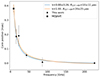 |
Fig. 2. Apparent core position as a function of frequency. Circles represent data from this research. The measurement at 8 GHz (square) was taken from Pushkarev et al. (2012) and was not used in the fit. The blue curve indicates the best fit of the form r = aν−1/kr + b using 227 GHz as the reference frequency. The orange curve represents the fit adopting the power law index kr = 1. The error bars include component position uncertainty as well as interpolation uncertainty at 15 and 43 GHz. R227 → BH is the angular distance between the 227 GHz core and the central BH. |
For the best fit, the coefficient is kr = 0.88 ± 0.26. Within the errors, it is indistinguishable from the kr = 1 expected in the case of a conical jet. The value of kr is consistent with the results of Lu et al. (2011), who obtained kr = 0.78 ± 0.29 between 15 and 86 GHz, using the latter as a reference frequency. Within an assumption that for infinite frequency the matter of the jet is totally transparent, we were able to locate the BH and establish the distance scale in the jet. For kr = 1, the BH is located 20 μas from the 227 GHz core, while for kr = 0.88 this angular distance is 10 μas. This value corresponds to 0.08 pc in the image plane, or 1.6 pc of distance along the jet. According to Kutkin et al. (2014) (Eq. 4), we calculated the magnetic field strength at a distance of 1 pc from the jet apex, B1 = 1.5 G, given the opening angle of the jet, ϕ = 0.5° (Pushkarev et al. 2009). We adopted the range of electron energies between γmin = 10 and γmax = 104. Since the magnetic field in the jet is likely toroidal and scales as B ∝ B1 r−1, we can calculate it at any distance along the jet. The distances to VLBI cores and magnetic field values at all frequencies are listed in Table 3. The uncertainty of the magnetic field is mainly propagated from the uncertainty of kr and is quite large. Improving the accuracy of component position measurements and extending frequency coverage in future experiments will help to improve these uncertainties and search for non-power-law dependence of the core position on frequency.
Magnetic field estimates from the core-shift measurements.
The distance between the apparent jet beginning at 86 GHz and 227 GHz falls below the level of uncertainty of the core position at these frequencies. This distance might be nonzero but too small to be firmly detected. On the other hand, at these high frequencies the apparent core might not be the surface of a unit optical depth, but rather a bright recollimation shock, which is discussed in Sects. 3.2 and 7. In this case, no core shift due to synchrotron opacity is expected at all.
The EHT array is currently undergoing developments to enable VLBI observations at 345 GHz (Doeleman et al. 2023; Raymond et al. 2024). It should be noted that within the model, if core-shift is nonzero between 227 GHz and 345 GHz, its amplitude would be Δr227 − 345 ≈ 4 μas and would likely not be measurable with the current EHT setup. However, spectral information in this frequency range would help us to deduce the real nature of the bright origin of the jet of NRAO 530 at 227 GHz and beyond.
3.2. Spectral properties
With multifrequency models aligned, we have access to the spectral information of individual components. We have identified which components describe the same spatial regions of the jet at different frequencies. Special regions of interest are: the apparent core at 86 and 227 GHz (components G1, W0); the apparent core at 43 GHz (G3, W1, Q0); and the apparent core at 15 GHz (W3, Q1, U0). All parameters of fit components are presented in Appendix C. In all of these regions, there are components at higher frequencies, coinciding with the apparent core at the lower one. The spectra for these regions are plotted in Fig. 3. We have checked for two sources of systematic effects that can affect derived spectral indices. Firstly, the sizes of model-fit components are not strictly equal at different frequencies. However, the difference in sizes is usually within the uncertainty of the measurements. Hence, we assume that at all frequencies corresponding components describe the same physical volume. Secondly, there might be a systematic uncertainty associated with flux scaling at 86 GHz, since zero-baseline VLBI flux density was scaled to that measured at ALMA. However, if ALMA catches some flux that is resolved at VLBI scales, then the flux of each component in the 86 GHz model should be lower. Hence, the spectral index of the 227 GHz core will remain that of the optically thin region regardless of the flux scaling uncertainties.
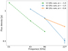 |
Fig. 3. Spectra of the core regions at 15, 43 GHz, and 86 GHz. |
Since we do not detect a significant core-shift between 86 and 227 GHz and the spectral index is negative (Sν ∝ να), we conclude that the jet matter is optically thin at these frequencies throughout the whole observed jet. In this case, the apparent core at 86 GHz and 227 GHz could be a standing shock feature, which makes it stand out in its brightness in comparison to the rest of the jet. If the apparent core at 345 GHz is co-spatial with that at 227 GHz, its flux density is estimated on the level of 0.2 Jy.
Since we use fit Gaussian components, we compare emission of the same volume in the jet at different frequencies. Hence, the measured spectral index is a proper proxy to the underlying power-law spectrum of the electron energy distribution. In both the 15 and 43 GHz core regions, the measured optically thin spectral index is α ≈ −1.4, which yields a steep electron energy spectrum, N(E) = N0E−p, with p = 1 − 2α = 3.8. The same argument yields p = 2.2 in the apparent core at 227 GHz, which requires rapid energy losses for the higher-energy electrons in the region between 1 and 10 pc from the BH.
4. Helical structure of the jet
The internal structure of the source, within a 1 mas radius, exhibits a curved jet with a downstream spiral structure. This pattern is likely due to either a precessing jet nozzle (e.g., Caproni et al. 2004; Fendt & Yardimci 2022) or instabilities within the jet itself, such as the Kelvin-Helmholtz (KH) instability (e.g., Ferrari et al. 1978; Perucho et al. 2004). To investigate these structures further, we utilized a three-dimensional helix model, denoted as H(A, λ, ϕ), which was fit to the measured positions of jet components. The parametric equation describing the helix model is given as follows:
where A is an amplitude, λ is a wavelength of the helix, ϕ is a phase, and d is the distance from the origin along the jet direction.
In order to account for distortion effects caused by the small viewing angle, θ = 3° (Jorstad et al. 2017; Weaver et al. 2022), of the jet, the helix model was projected onto the sky plane prior to fitting, incorporating an additional parameter, the jet position angle, Ψ, to account for the average position angle of the jet. The complete model is defined as

where R(Ψ) and R(θ) are rotational matrices. We employed bootstrapping to obtain probability distributions and confidence intervals for the parameters.
It is important to note that although the helix structure appears to be similar in both the instability and precession cases, these patterns arise from distinct phenomena. Consequently, different assumptions were made for each case, requiring modification of Eq. (3). In the case of a precession-based pattern, we assume that all jet matter trajectories were ballistic. Therefore, in snapshot images one sees a narrow curved jet, contained within a wider cone. The fit precession-helix should increase its amplitude with distance with a linear law, A ∝ d, and have constant wavelength, λ.
In the other case, the amplitude of the helix grows proportionally to the jet radius, Rjet. Thus, the amplitude and the wavelength of the helix should mirror the jet geometry profile. Consequently, A ∝ dk, λ ∝ dk, where k is determined by the jet expansion profile, Rjet ∝ dk (Hardee 2000; Lobanov et al. 2003). Since we used combined data from all five frequencies together for fitting, we assigned a weight for each data point, W, which depends on the flux density, F, size, S, and observed frequency of the component. Thus, W = F(ν/ν0)−αS−1, where we chose the spectral index α = −0.75, which is a common value in AGN jets. In this case, the spectral index value does not correspond to a steeper one estimated from the VLBI cores of the current observations where α ≈ −1.5 (Fig. 3). However, since steeper spectra do not change weights significantly, we decided to take a more conservative value, which is supported by MOJAVE observations Hovatta et al. (2014) at 8 and 15 GHz. The final fitting results are shown in Table 4 and Fig. 4.
Parameters of helices in precession and KH instability cases.
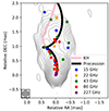 |
Fig. 4. NRAO 530 jet stack intensity CLEAN image at 43 GHz, with positions of the Gaussian modelfit components overlaid by the precession model (black curve) and the KH instability model (pink curve). All image model components are displayed here as same-size circles for clarity. The colors correspond to frequencies 15, 22, 43, 86, and 227 GHz, as in Fig. 1. The stacked 43 GHz intensity map is presented here with contours at increasing powers of 2, starting from 3 mJy/beam. The map peak is 1.6 Jy/beam. The CLEAN beam is shown in the lower left corner as a 0.25 mas circle. The stacked map was made using component-based method alignment within 14 years (60 epochs) of observations by the BU Blazar program. |
5. Brightness temperature
After decomposing the source structure into distinct Gaussian components, we can directly calculate the observed brightness temperature for each of them using Eq. (5),
where kB is the Boltzmann’s constant, S the component flux density, λ the wavelength, δ the Doppler-factor, z the redshift, and θ the angular size of the component, defined as the maximum of the full width at half maximum (FWHM) of the fit Gaussian and the resolution limit (Lobanov 2005). Since we have aligned all single-frequency models of the source, we can study how the brightness temperature changes along the jet, as is shown in Fig. 5.
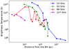 |
Fig. 5. Observed brightness temperature of model components as a function of the position along the jet, de-projected. Colors represent different frequencies. |
Equation (5) implies that the brightness temperature at a given distance from the central engine depends on the spectral index as Tb ∝ ν−2 + α, if optically thin synchrotron emission is assumed. A two-order difference between the brightness temperatures values at 43 and 227 GHz at 10 pc implies that α ≈ −1.2. This is consistent with the optically thin part of the spectrum of the 43 GHz core region, α = −1.5 (blue line in Fig. 3).
15 and 43 GHz analysis of the brightness-temperature gradients in a sample of 28 AGNs show that they generally are well described by a single power law Burd et al. (2022, Kravchenko et al., in prep.). This is applicable in the assumption of a straight constant-speed jet with a power-law distribution of the magnetic field and the particle density along the outflow. Regular deviation of the decline in Tb from a pure power-law dependency seen in NRAO 530 in Fig. 5 indicates a departure from this scenario. We suggest that a change in the local orientation of the jet, resulting in variations in the viewing angle of 2° < θ < 4° due to precession, leads to a change in the Doppler factor, and hence causes a nonlinear gradient of the brightness temperature with the distance along the jet.
6. Linear polarization and rotation measure structure
Polarimetric images of NRAO 530 at 15, 43, and 86 GHz are shown in Fig. 6, along with the 227 GHz EHT image. The structure is dominated by the core and the jet that is visible at low frequencies. At 15 GHz, the jet polarization is characterized by a two-sided structure, which is also marginally detected at 43 GHz. The fractional polarization in the jet center is of a few percent and increases up to 50 percent toward the jet edges. The latter fractional polarization is partially caused by systematic errors of the CLEAN procedure that can be corrected for from the results of simulations (Pushkarev et al. 2023). Linearly polarized emission in the inner ∼0.2 mas is represented by an extended region at 86 GHz, which is resolved into two separate components at 227 GHz. At all frequencies, fractional polarization is weak in the core region (about 2%) and increases up to 30% downstream and toward the jet edges.
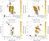 |
Fig. 6. Total intensity and linear polarization 15, 43, 86, and 227 GHz CLEAN images. Color denotes the distribution of the fractional linear polarization overlaid with the sticks indicating the electric polarization vector directions, not corrected for Faraday rotation. A synthesized beam is shown by a shaded ellipse in the lower left corner and its size is given. The Stokes I contours are plotted at increasing powers of 4, starting from the corresponding 3 rms level. The P contours are drawn at a 4 rms level. Here, we plot interpolated 15 and 43 GHz images (see Sect. 2.6 for details). The original MOJAVE and BU-BLAZAR images are given in Appendix B. |
Multiwavelength observations can be combined to obtain a Faraday RM image of NRAO 530. The RM was determined by χ = χ0 + RM × λ2, where λ is the observed wavelength, and χ0 and χ are the intrinsic and observed EVPA of the emitting region, respectively. Broad frequency coverage enables us to construct RM maps over a range of scales. Due to a progressively larger difference in the wavelengths that leads to the significant smearing of polarized structure when restoring with the large beam size, in the RM analysis we considered separately two frequency ranges: 15−43 GHz and 43−227 GHz. For the 43−86−227 GHz range, the images were tapered and convolved with a common circular beam size of 0.1 mas, which slightly over-resolves the 43 GHz image, while still preserving a fraction of the higher resolution achieved at 86 GHz and 227 GHz. Images at different frequencies were aligned using map shifts quoted in Table 2.
In the RM analysis, we considered only pixels in the images for which linearly polarized intensity at all frequencies was more than three times the rms. The RM map was computed by performing a linear fit to the dependence of the EVPA(λ2) at each pixel, blanking pixels with a poor fit based on a χ2 criterion. The χ2 of the fit was calculated using the formula
where N is the number of data points, Oi are the observed data, Ei are the expected data based on the model, and σi is the measurement error of the individual data point.
Since 22 GHz data is single polarization and cannot be used in this analysis, the χ − λ2 alignment between two frequencies of 15 and 43 GHz is subject to ±nπ-ambiguity. Considering the value of the 86 GHz EVPA integrated over an image, we see a robust linear dependence over 15−86 GHz, which implies that there is no ±nπ EVPA rotation to be made.
The resultant RM map in the 15−43 GHz range with λ2-fits at four locations in the jet are given in Fig. 7. The RM values in the core (associated with the self-synchrotron absorbed region) amount to ∼ − 3000 rad m−2, which decreases to a few hundred rad m−2 downstream, in both the eastern and western parts of the jet.
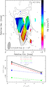 |
Fig. 7. Faraday RM at low frequencies. (Top panel) 15−43 GHz RM map with 43 GHz total intensity contours at increasing powers of 2, lowest contour 1.40 mJy beam−1. Sticks denote linear polarization orientation at 43 GHz corrected for Faraday rotation. Numbers indicate locations where the EVPA(λ2)-fits (bottom panel) are taken. Faraday rotation regression is shown by lines, and estimated values are given in rad m−1. |
The RM value in the jet is comparable with 371 rad m−2 estimated by Hovatta et al. (2012) in the frequency range of 8−15 GHz. There is an indication on the RM map of Hovatta et al. (2012) for RM of about −700 rad m−2 toward the core region. This value is consistent with our measurements; however, we probed this region in more detail. Our RM values are in good agreement with the multiwavelength polarimetric observations of NRAO 530 by Chen et al. (2010), who estimated RM of −1062 ± 0.2 rad m−2 between 15 and 43 GHz.
The 43−227 GHz RM map with λ2-fits at four locations in the jet are shown in Fig. 8. We estimate an RM value in the inner region of ∼ − 4 × 10⁴ rad m−2. Goddi et al. (2021) provide RM estimates of ( − 2.1 ± 0.6)×104 rad m−2 at 3 mm, which is comparable to the inter-band RM between 1 and 3 mm (−3.3 × 10⁴ rad m−2). These and our RM estimates are also in agreement with the values RM = ( − 3.1 ± 1.3)×104 rad m−2 at 1.3 mm reported by Bower et al. (2018).
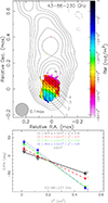 |
Fig. 8. Faraday RM at high frequencies. (Top panel) 43−227 GHz rotation measure map with 86 GHz total intensity contours at increasing powers of 2, lowest contour 3.34 mJy beam−1. Sticks denote linear polarization orientation at 86 GHz corrected for Faraday rotation. Numbers indicate locations where the EVPA(λ2) fits (bottom panel) are taken. Faraday rotation regression is shown by lines, and estimated values are given in rad m−1. |
In Fig. 9, we plot the map of χ2 values obtained from the EVPA-λ2 fit. We fit a two-parameter model to three data points, and therefore we have 1 degree of freedom. From the χ2 distribution, the corresponding 95% confidence limit is χ2 < 3.841. Linear fits of χ versus λ2 are found in all pixels for which linearly polarized intensity in all bands was higher than three times its rms. The observed large value of RM is consistent with the rotating medium being external to the emitting region. To our knowledge, this is the first RM map of NRAO 530 obtained at such high frequencies in VLBI observations.
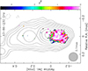 |
Fig. 9. Map of χ2 values of the EVPA-λ2 fit for the frequency range 43−227 GHz. Gray contours are the same as in Fig. 8. |
Jorstad et al. (2007) derived the following relation of RM as a function of frequency for a conical jet under equipartition |RM|∝νa, where the value of a depends on the power-law change in the electron density, ne, as a function of distance, r, from the BH, ne ∝ r−a. Typical values obtained in the literature vary in the range a = 1 − 4 (Jorstad et al. 2007; Algaba 2013; Kravchenko et al. 2017), while the value a = 2 would imply that the Faraday rotation is occurring in a sheath around a conically expanding jet. For NRAO 530, the linear fit between our 15−43 GHz and 43−227 GHz RM estimates in the core region results in a ∼ 1.7, consistent with the model of a sheath surrounding a conically expanding flow. In the source frame, RMint = (1 + z)2RM. Given that z = 0.902, RMint ∼ 105 rad m−2.
Intrinsic orientation of polarization (corrected for the RM) is shown in Figs. 7 and 8. The EVPAs at centimeter wavelengths point toward the external region of the jet in a fountain-like pattern. Zero polarization along the jet spine, visible in Fig. 6 and in the stack 15 GHz images of NRAO 530 (Pushkarev et al. 2023), is accompanied by a high variability of EVPAs observed on a time interval of two decades (Zobnina et al. 2023). Jorstad et al. (2017) estimate an intrinsic viewing angle of δ0 > 60°, which suggests a helical magnetic field pitch angle for this source of γ0 ∼ 40 − 70°.
As we point out in Sect. 4, the jet appears wide at 1 mas from the core, most likely due to the intrinsic changes in the jet direction amplified by the projection effects (see Fig. 4). In this case, an intrinsically narrow relativistic jet is precessing inside a wider cone cleared by the jet itself. The RM, taken transverse the outflow direction at 1.1 mas down from the core, changes its value (Fig. 10). Although transverse RM values do not cross zero, almost monotonic behavior of RM transverse to the jet hints at the presence of the helical magnetic field in the plasma outside of the wide cone, similar to that discovered in 3C 273 by Lisakov et al. (2021). The scenario of a precessing jet threaded by the helical magnetic field can also explain the observed polarization structure with the EVPAs pointing toward jet edges, accompanied by a low polarization and high variability of EVPAs along the jet spine (Todorov et al. 2024). In this scenario, due to the limited resolution of the VLBI observations, the initially strong polarization along the jet spine is smeared in the projection to the sky due to the overlap of regions with the different EVPA orientations.
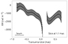 |
Fig. 10. Transverse slice taken across the RM map (Fig. 7) at 1.1 mas. The black dots show the RM fit at every pixel across the slice, with the gray area indicating the error in the fit for each point. |
7. Discussion
7.1. Support for the presence of component C2
Data at 227 GHz provide a hint of the dim C2 component, the most downstream one (see Fig. 5 of Jorstad et al. 2023). However, it was detected with DIFMAP, EHT-IMAGING, and DMC, but not with SMILI or THEMIS. We have found a counterpart of this component at other frequencies; namely, at 86 GHz and 43 GHz. A zoom-in map of the region is presented in Fig. 11. Here, for 227 GHz we adopted naming from Jorstad et al. (2023). It is apparent that the component C2 at 227 GHz spatially coincides with the core of the 43 GHz jet and component W1 from the 86 GHz jet. It corroborates the detection of C2 that was made with 227 GHz data only.
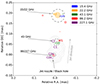 |
Fig. 11. Central region of NRAO 530. Contours represent total intensity at 227 GHz. Model components at 227 GHz are named according to Jorstad et al. (2023), at other frequencies – according to Table C.1. The size of Gaussian components is reduced by a factor of five with respect to Fig. 1 for visual clarity. Dashed circles show the location of the apparent VLBI core at different frequencies according to the labels. Component C2 spatially coincides with the apparent core of the 43 GHz model Q0 and an 86 GHz component W1. A weak component, C0b, spatially coincides with the true jet origin calculated using core shift. |
7.2. Jet structure and its evolution in two possible scenarios
The jet structure analysis can reveal intrinsic physical parameters. In the first scenario of precession, one can evaluate the period and the opening angle, α, of the precession cone. The opening angle was obtained directly from the fit helix, and thus α = 3° ±1°. In the assumption of ballistic trajectories of plasma in a jet, we can estimate the distance of a one-period turn of a precessing jet, dperiod ≈ λproj = 1.6 ± 0.5 mas (Table 4). Using a weighted average Lorenz factor of Γ = 8.9 ± 2.5 (Jorstad et al. 2017), we found an apparent speed of βapp ≈ 7, which corresponds to an angular speed of μ ≈ 0.3 mas/yr. We estimated the period of precession, P = dperiod/βapp = 6 ± 4 yr, which does not contradict the case in which the precession is initiated by a double supermassive BH system like in OJ 287 (Sillanpaa et al. 1988; Valtonen et al. 2009; Britzen et al. 2018; Gómez et al. 2022) or M 81 (Martí-Vidal et al. 2011; von Fellenberg et al. 2023). The result corresponds to the period found in the radio light curve (An et al. 2013). An additional support for the obtained period can be demonstrated by the 14-year stack image of the jet at 43 GHz (Fig. 4). The image shows a symmetrical jet experiencing a dramatic expansion until 1 mas, which is the result of a smearing effect produced by the time-variable jet position angle. Since the stack time is more than twice the length of the obtained period, the precession is a feasible interpretation of the observed phenomena. The parameters were derived assuming ballistic trajectories, implying the conical geometry of the jet’s precession cone. However, if the expansion parameter of the fit model (Eq. 4) is free, the fitting yields k = 0.8 ± 0.1 (Table 4), which deviates from the conical shape but provides the best fit to the data. Nevertheless, it does not change the obtained precession period significantly. On the one hand, deviation from the conical shape can be induced by limited and localized data points with high accuracy, providing measurements of less than one wavelength. Additionally, real physical phenomena like jet nutation or nonuniform local hydrodynamic conditions can provide an apparent or real distortion of the jet shape.
In the second scenario, we assume that the KH instability plays a leading role in forming the helical pattern. From the fitting results, the expansion index, k = 0.5 ± 0.2 (Table 4), does not correspond to the local visible hyperbolic expansion, but agrees with the global parabolic geometry of the jet at 15 GHz (Pushkarev et al. 2017). We used linear analysis (Hardee 2000; Lobanov et al. 2003; Vega-García et al. 2020) to identify and obtain the basic physical parameters of the jet. The measurements made in Sect. 4 show a single wiggling ridge line that can be identified as a helical surface instability mode with a wavelength of λ/Rjet = 13 ± 10. Using the apparent speed, the viewing angle listed in the previous paragraph, and a pattern speed of βwapp, we estimated the Mach number, Mj, and the ratio of the jet to the ambient density, η (Vega-García et al. 2020). However, the pattern speed, βwapp, is complicated to obtain using existing observations, since a much greater sensitivity to a faint extended structure and resolution is needed. In the case of M87, the pattern speed was found using wavelet-based analysis and βwapp ≈ 0.3 (Mertens et al. 2016). In the case of NRAO 530, the same type of analysis is unfeasible; thus, the best estimation for the pattern speed will be sub-relativistic speeds of ∼0.5c (Hardee & Norman 1988; Norman & Hardee 1988; Hardee 2000). Using this set of parameters, the unrealistically large η ≈ 0.8 was found. That means that the βwapp estimation is too large. For example, in relativistic jet simulations, Mjet ∼ 3, η ∼ 0.01 − 0.1 (Norman & Hardee 1988; Perucho et al. 2005; Perucho & Martí 2007). To achieve physical η ∼ 0.01 − 0.1, βwapp ≈ 0.1 − 0.2 is needed. Finally, using βwapp = 0.1 we obtained the Mach number Mj = 4 ± 3 and the density ratio η = 0.03 ± 0.07.
To show how the KH pattern corresponds to the observed stacked image, we calculated the apparent pattern speed of βwapp ≈ 0.006. Using the same dproj from the precession case, we obtained an observed period of instability pattern of Pobs ∼ 5000 years. The analysis shows that KH instability cannot provide such a rapid pattern change as precession. Even if βwapp = 0.5 were considered, Pobs ∼ 600 years. In any case, the instability pattern will not create a smeared picture within 14 years.
It should be noted that even though the precession scenario is better supported by our observations, it has its own shortcomings. For instance, if precession is the only mechanism driving the jet wobbling, then all model components should follow ballistic trajectories. As is shown by Weaver et al. (2022), in the innermost 1 mas from the core, components move along straight trajectories (see Fig. F1). However, farther from the core trajectories of some components are clearly non-ballistic, which is also supported by Lister et al. (2019) at 15 GHz. This discrepancy should be investigated further. We shall dedicate a future publication to a detailed analysis of temporal variations in the jet structure and its direction.
7.3. Magnetic field in and around the jet
Polarimetric images, Fig. 6 in this paper and those presented by Jorstad et al. (2023), show that at 15 GHz EVPA is perpendicular to the jet direction in the core region, while at higher frequencies EVPA are approximately parallel to the jet. This could be interpreted within the assumption that the toroidal component of magnetic field dominates in the innermost portion of the jet in NRAO 530 and 90° rotation of the electric vector is solely ascribed to different opacities of the jet matter at different frequencies. Namely, at 86 GHz and 227 GHz, the core is shown to be optically thin (see Sect. 3). This is well supported by findings of Gómez et al. (2016), who also found the magnetic field to remain toroidal in the inner jet of BL Lac. In this case, we assume that the toroidal configuration of the magnetic field could persist even close to the central BH, and hence one can extrapolate the magnetic field strength toward the BH using the B ∝ r−1 relation.
Within this assumption, magnetic field strength at 5 Rg is B = 3000 − 30 000 G, depending on the BH mass in the range 2 − 0.2 × 10⁹ M⊙ (Liang & Liu 2003; Keck 2019). This range of BH masses corresponds to 5 Rg = 100 − 10 AU. The magnetic field values are at least two orders of magnitude higher than those reported by EHT Collaboration (2021b) in M87 at the same distance. If we compare the jet luminosity, Lν = 4πDLνFν, at some frequency where synchrotron emission of the jet dominates and Doppler boosting can be measured, say at 15 GHz, NRAO 530 appears 1000 times brighter than M87. This difference could largely be attributed to the difference in magnetic field strength.
On the other hand, Kino et al. (2022) estimated a magnetic field of 200 − 5000 G at the horizon of the BH in M87. Magnetic fields on the order of 1000 G are also required in the arguments provided by Blandford et al. (2019). Future polarimetric observations of M87 and NRAO 530 at both 227 GHz and 345 GHz will help to better account for the magnetic field difference in the models of jet launching (Johnson et al. 2023).
Linear polarization structure of NRAO 530 downstream of the jet at 15 and 43 GHz shows limb brightening structure, with the electric vectors pointing toward the jet’s edges. The fractional polarization along the jet spine is almost zero, which is accompanied by a high variability of the EVPAs along the jet center that is observed over a two-decade time interval (Zobnina et al. 2023). Such behavior can be explained well by the model of a jet threaded by the helical magnetic field precessing at a time interval of ten years (Todorov et al. 2024). Due to the small viewing angle, the averaging of jet images that captured a different jet direction will lead to the overlapping of polarization with different orientations. As a result, the observed polarized intensity in the center of the jet will be smeared and will be accompanied by an increased variability of EVPA in this area.
Substantial variations in the position angle of the jet components observed in the significant number of AGN jets (Lister et al. 2021) and large apparent jet opening angles (Pushkarev et al. 2017) serve as the basis for this scenario. Moreover, there is an increasing number of sources for which a possible connection between the variation in the intensity or jet position angle with precession has been shown (e.g., Britzen et al. 2018; Cui et al. 2023; Britzen et al. 2023; Algaba et al. 2019).
We also note that the values of the Faraday RM at 43−227 GHz increase in absolute values downstream of the jet (see Fig. 8). This behavior is in contrast with an expected gradual decrease in the RM magnitude due to decreasing magnetic field strength and particle density of the rotating medium surrounding the jet. However, according to the precession model, in the region of interest the jet viewing angle increases approximately from 2.3° to 3.1°. Therefore, the path length in the rotating medium is increased, increasing RM values. Alternatively, we might be able to resolve small scale inhomogeneities in the Faraday screen that likely occur at the probed distance of only 1 pc from the central engine. Multifrequency observations of NRAO 530 at other precession phases are required to test these hypotheses.
7.4. Jet beginning
According to our multifrequency model of the jet in NRAO 530, we can associate its real starting point with the component C0b at 227 GHz (see Fig. 11). As we show in Sect. 3.2, the jet is transparent at 227 GHz (460 GHz in the source frame) and we can indeed detect emission down to the BH. The flux density of this component, FC0b = 67 mJy, can be compared with the total flux of the M87 ring from ETH observations EHT Collaboration (2019), Fring ≈ 1 Jy. According to Lu et al. (2023), the ring is indeed the brightest feature in the innermost jet. Taking into account the difference in distance, frequency shift, and spectrum, the intrinsic luminosity of the C0b feature of NRAO 530 is 104 times higher than the total flux of the M87 ring. Given the difference of the same order in the magnetic field strength near the BHs of M87 and NRAO 530, we might indeed probe the same region around the BH with our observations at 227 GHz. Future observations of NRAO 530 at 227 and 345 GHz will be required to answer this question.
8. Conclusions
We have analyzed quasi-simultaneous observations of the blazar NRAO 530 at frequencies 15, 22, 43, 86, and 227 GHz performed around April 2017.
-
The relatively dim component C2 identified at 227 GHz by Jorstad et al. (2023) spatially coincides with the apparent core at 43 GHz and optically thin component at 86 GHz.
-
We found that the jet exhibits a spiral pattern, which is most likely attributed to the precession of the jet nozzle with a period of 6 ± 4 years.
-
With core-shift analysis, we have shown that the matter of the jet might be completely transparent at frequencies above 86 GHz. However, further EHT observations at 345 GHz are required to test this result. The apparent core at 345 GHz should have a flux density of S345 ≈ 200 mJy and should be located no farther than 4 μas from the core at 227 GHz.
-
We estimate the strength of the magnetic field close to the central BH to be 3 × (103 − 104) G, much stronger than that derived by direct observations of the M87* BH shadow at the same distance.
-
For the first time, we have revealed the structure of Faraday RM and obtained its amplitude using VLBI polarimetric observations between 43, 86, and 227 GHz. The largest value we detected is −48 000 rad/m2.
-
With fine resolution at 227 GHz, core shift analysis, and estimates of the magnetic field strength, we conclude that the component C0b with the flux density of 67 mJy could represent the disk around the BH or a bright feature in the innermost jet; for instance, a recollimation shock wave.
Acknowledgments
The authors thank Andrei Lobanov and two anonymous referees for reviewing the manuscript. M2FINDERS project has received funding from the European Research Council (ERC) under the European Union’s Horizon 2020 research and innovation programme (grant agreement No. 101018682). This research has made use of data obtained with the Global Millimeter VLBI Array (GMVA), coordinated by the VLBI group at the Max-Planck-Institut für Radioastronomie (MPIfR). The GMVA consists of telescopes operated by the MPIfR, IRAM, Onsala, Metsähovi, Yebes, the Korean VLBI Network, the Green Bank Observatory and the Very Long Baseline Array (VLBA). The VLBA and the GBT are a facility of the National Science Foundation operated under cooperative agreement by Associated Universities, Inc. The data were correlated at the VLBI correlator of the MPIfR in Bonn, Germany. This paper uses data obtained with the 100 m radiotelescope of the MPIfR at Effelsberg. This research has made use of data from the MOJAVE database that is maintained by the MOJAVE team (Lister et al. 2018). This study makes use of VLBA data from the VLBA-BU Blazar Monitoring Program (BEAM-ME and VLBA-BU-BLAZAR http://www.bu.edu/blazars/VLBA_GLAST/1730.html), funded by NASA through the Fermi Guest Investigator Program. The VLBA is an instrument of the National Radio Astronomy Observatory. The National Radio Astronomy Observatory is a facility of the National Science Foundation operated by Associated Universities, Inc. ALMA is a partnership of the European Southern Observatory (ESO; Europe, representing its member states), NSF, and National Institutes of Natural Sciences of Japan, together with National Research Council (Canada), Ministry of Science and Technology (MOST; Taiwan), Academia Sinica Institute of Astronomy and Astrophysics (ASIAA; Taiwan), and Korea Astronomy and Space Science Institute (KASI; Republic of Korea), in cooperation with the Republic of Chile. The Joint ALMA Observatory is operated by ESO, Associated Universities, Inc. (AUI)/NRAO, and the National Astronomical Observatory of Japan (NAOJ). We also gratefully acknowledge the support provided by the extended staff of the ALMA, both from the inception of the ALMA Phasing Project through the observational campaigns since 2017.
References
- Abdollahi, S., Acero, F., Ackermann, M., et al. 2020, ApJS, 247, 33 [Google Scholar]
- Algaba, J. C. 2013, MNRAS, 429, 3551 [Google Scholar]
- Algaba, J. C., Rani, B., Lee, S. S., et al. 2019, ApJ, 886, 85 [NASA ADS] [CrossRef] [Google Scholar]
- Aller, H. D., Aller, M. F., Latimer, G. E., et al. 1985, ApJS, 59, 533 [Google Scholar]
- An, T., Baan, W. A., Wang, J.-Y., et al. 2013, MNRAS, 434, 3487 [Google Scholar]
- Blackburn, L., Chan, C.-K., Crew, G. B., et al. 2019, ApJ, 882, 23 [Google Scholar]
- Blandford, R., Meier, D., & Readhead, A. 2019, ARA&A, 57, 467 [NASA ADS] [CrossRef] [Google Scholar]
- Bower, G. C., Broderick, A., Dexter, J., et al. 2018, ApJ, 868, 101 [NASA ADS] [CrossRef] [Google Scholar]
- Britzen, S., Fendt, C., Witzel, G., et al. 2018, MNRAS, 478, 3199 [NASA ADS] [Google Scholar]
- Britzen, S., Zajaček, M., Gopal-Krishna, et al. 2023, ApJ, 951, 106 [CrossRef] [Google Scholar]
- Burd, P. R., Kadler, M., Mannheim, K., et al. 2022, A&A, 660, A1 [NASA ADS] [CrossRef] [EDP Sciences] [Google Scholar]
- Caproni, A., Mosquera Cuesta, H. J., & Abraham, Z. 2004, ApJ, 616, L99 [Google Scholar]
- Casadio, C., Marscher, A., Jorstad, S., et al. 2019, A&A, 622, A158 [NASA ADS] [CrossRef] [EDP Sciences] [Google Scholar]
- Chael, A. A., Johnson, M. D., Bouman, K. L., et al. 2018, ApJ, 857, 23 [Google Scholar]
- Chen, Y. J., Shen, Z. Q., & Feng, S. W. 2010, MNRAS, 408, 841 [Google Scholar]
- Cho, I., Zhao, G.-Y., Kawashima, T., et al. 2022, ApJ, 926, 108 [NASA ADS] [CrossRef] [Google Scholar]
- Cui, Y.-Z., Hada, K., Kino, M., et al. 2021, RAA, 21, 205 [Google Scholar]
- Cui, Y., Hada, K., Kawashima, T., et al. 2023, Nature, 621, 711 [NASA ADS] [CrossRef] [Google Scholar]
- Doeleman, S. S., Barrett, J., Blackburn, L., et al. 2023, Galaxies, 11, 107 [NASA ADS] [CrossRef] [Google Scholar]
- EHT Collaboration (Akiyama, K., et al.) 2019, ApJ, 875, L3 [Google Scholar]
- EHT Collaboration (Akiyama, K., et al.) 2021a, ApJ, 910, L12 [Google Scholar]
- EHT Collaboration (Akiyama, K., et al.) 2021b, ApJ, 910, L13 [Google Scholar]
- EHT Collaboration (Akiyama, K., et al.) 2022a, ApJ, 930, L12 [NASA ADS] [CrossRef] [Google Scholar]
- EHT Collaboration (Akiyama, K., et al.) 2022b, ApJ, 930, L13 [NASA ADS] [CrossRef] [Google Scholar]
- Fendt, C., & Yardimci, M. 2022, ApJ, 933, 71 [NASA ADS] [CrossRef] [Google Scholar]
- Ferrari, A., Trussoni, E., & Zaninetti, L. 1978, A&A, 64, 43 [NASA ADS] [Google Scholar]
- Fomalont, E. B. 1999, ASP Conf. Ser., 180, 301 [NASA ADS] [Google Scholar]
- Goddi, C., Martí-Vidal, I., Messias, H., et al. 2019, PASP, 131, 075003 [Google Scholar]
- Goddi, C., Martí-Vidal, I., Messias, H., et al. 2021, ApJ, 910, L14 [NASA ADS] [CrossRef] [Google Scholar]
- Gómez, J. L. 2002, VLBA Scientific MEMO (Socorro: NRAO) [Google Scholar]
- Gómez, J. L., Lobanov, A. P., Bruni, G., et al. 2016, ApJ, 817, 96 [Google Scholar]
- Gómez, J. L., Traianou, E., Krichbaum, T. P., et al. 2022, ApJ, 924, 122 [Google Scholar]
- Hada, K., Park, J. H., Kino, M., et al. 2017, PASJ, 69, 71 [NASA ADS] [CrossRef] [Google Scholar]
- Hardee, P. E. 2000, ApJ, 533, 176 [Google Scholar]
- Hardee, P. E., & Norman, M. L. 1988, ApJ, 334, 70 [Google Scholar]
- Hovatta, T., Lister, M. L., Aller, M. F., et al. 2012, AJ, 144, 105 [Google Scholar]
- Hovatta, T., Lister, M. L., Aller, H. D., et al. 2014, AJ, 147, 143 [NASA ADS] [CrossRef] [Google Scholar]
- Issaoun, S., Johnson, M. D., Blackburn, L., et al. 2019, ApJ, 871, 30 [Google Scholar]
- Issaoun, S., Wielgus, M., Jorstad, S., et al. 2022, ApJ, 934, 145 [NASA ADS] [CrossRef] [Google Scholar]
- Istomin, Y. N., & Pariev, V. 1996, MNRAS, 281, 1 [Google Scholar]
- Janssen, M., Goddi, C., van Bemmel, I. M., et al. 2019, A&A, 626, A75 [NASA ADS] [CrossRef] [EDP Sciences] [Google Scholar]
- Johnson, M. D., Akiyama, K., Blackburn, L., et al. 2023, Galaxies, 11, 61 [NASA ADS] [CrossRef] [Google Scholar]
- Jorstad, S. G., Marscher, A. P., Stevens, J. A., et al. 2007, AJ, 134, 799 [NASA ADS] [CrossRef] [Google Scholar]
- Jorstad, S. G., Marscher, A. P., Morozova, D. A., et al. 2017, ApJ, 846, 98 [Google Scholar]
- Jorstad, S., Wielgus, M., Lico, R., et al. 2023, ApJ, 943, 170 [NASA ADS] [CrossRef] [Google Scholar]
- Junkkarinen, V. 1984, PASP, 96, 539 [NASA ADS] [CrossRef] [Google Scholar]
- Keck, M. 2019, Ph.D. Thesis, Boston University [Google Scholar]
- Kellermann, K. I., Vermeulen, R. C., Zensus, J. A., & Cohen, M. H. 1998, AJ, 115, 1295 [NASA ADS] [CrossRef] [Google Scholar]
- Kharb, P., Lister, M. L., & Cooper, N. J. 2010, ApJ, 710, 764 [NASA ADS] [CrossRef] [Google Scholar]
- Kino, M., Takahashi, M., Kawashima, T., et al. 2022, ApJ, 939, 83 [NASA ADS] [CrossRef] [Google Scholar]
- Konigl, A. 1981, ApJ, 243, 700 [Google Scholar]
- Kravchenko, E. V., Kovalev, Y. Y., & Sokolovsky, K. V. 2017, MNRAS, 467, 83 [NASA ADS] [Google Scholar]
- Kutkin, A. M., Sokolovsky, K. V., Lisakov, M. M., et al. 2014, MNRAS, 437, 3396 [Google Scholar]
- Leppänen, K., Zensus, J., & Diamond, P. 1995, AJ, 110, 2479 [CrossRef] [Google Scholar]
- Liang, E. W., & Liu, H. T. 2003, MNRAS, 340, 632 [NASA ADS] [CrossRef] [Google Scholar]
- Lisakov, M. M., Kovalev, Y. Y., Savolainen, T., Hovatta, T., & Kutkin, A. M. 2017, MNRAS, 468, 4478 [Google Scholar]
- Lisakov, M. M., Kravchenko, E. V., Pushkarev, A. B., et al. 2021, ApJ, 910, 35 [NASA ADS] [CrossRef] [Google Scholar]
- Lister, M. L., Aller, M. F., Aller, H. D., et al. 2018, ApJS, 234, 12 [CrossRef] [Google Scholar]
- Lister, M. L., Homan, D. C., Hovatta, T., et al. 2019, ApJ, 874, 43 [NASA ADS] [CrossRef] [Google Scholar]
- Lister, M. L., Homan, D. C., Kellermann, K. I., et al. 2021, ApJ, 923, 30 [NASA ADS] [CrossRef] [Google Scholar]
- Lobanov, A. P. 1998, A&A, 330, 79 [NASA ADS] [Google Scholar]
- Lobanov, A. P. 2005, ArXiv e-prints [arXiv:astro-ph/0503225] [Google Scholar]
- Lobanov, A., Hardee, P., & Eilek, J. 2003, New Astron. Rev., 47, 629 [CrossRef] [Google Scholar]
- Lu, R. S. 2010, Ph.D. Thesis, der Mathematisch-Naturwissenschaftlichen Fakultät der Universität zu Köln [Google Scholar]
- Lu, R. S., Krichbaum, T. P., & Zensus, J. A. 2011, MNRAS, 418, 2260 [NASA ADS] [CrossRef] [Google Scholar]
- Lu, R.-S., Asada, K., Krichbaum, T. P., et al. 2023, Nature, 616, 686 [CrossRef] [Google Scholar]
- Martí-Vidal, I., Marcaide, J. M., Alberdi, A., et al. 2011, A&A, 533, A111 [NASA ADS] [CrossRef] [EDP Sciences] [Google Scholar]
- Mertens, F., Lobanov, A., Walker, R., & Hardee, P. 2016, A&A, 595, A54 [NASA ADS] [CrossRef] [EDP Sciences] [Google Scholar]
- Mizuno, Y., Lyubarsky, Y., Nishikawa, K.-I., & Hardee, P. E. 2012, ApJ, 757, 16 [Google Scholar]
- Narayan, R., Li, J., & Tchekhovskoy, A. 2009, ApJ, 697, 1681 [NASA ADS] [CrossRef] [Google Scholar]
- Niinuma, K., Lee, S.-S., Kino, M., & Sohn, B. W. 2015, Publ. Korean Astron. Soc., 30, 637 [Google Scholar]
- Norman, M. L., & Hardee, P. E. 1988, ApJ, 334, 80 [NASA ADS] [CrossRef] [Google Scholar]
- Park, J., Hada, K., Kino, M., et al. 2019, ApJ, 887, 147 [Google Scholar]
- Perucho, M., & Martí, J. M. 2007, MNRAS, 382, 526 [NASA ADS] [CrossRef] [Google Scholar]
- Perucho, M., Hanasz, M., Martí, J. M., & Sol, H. 2004, A&A, 427, 415 [NASA ADS] [CrossRef] [EDP Sciences] [Google Scholar]
- Perucho, M., Lobanov, A. P., & Martí, J. M. 2005, Mem. Soc. Astron. Ital., 76, 110 [Google Scholar]
- Planck Collaboration XIII. 2016, A&A, 594, A13 [NASA ADS] [CrossRef] [EDP Sciences] [Google Scholar]
- Pushkarev, A. B., Kovalev, Y. Y., Lister, M. L., & Savolainen, T. 2009, A&A, 507, L33 [NASA ADS] [CrossRef] [EDP Sciences] [Google Scholar]
- Pushkarev, A. B., Hovatta, T., Kovalev, Y. Y., et al. 2012, A&A, 545, A113 [NASA ADS] [CrossRef] [EDP Sciences] [Google Scholar]
- Pushkarev, A. B., Kovalev, Y. Y., Lister, M. L., & Savolainen, T. 2017, MNRAS, 468, 4992 [Google Scholar]
- Pushkarev, A. B., Aller, H. D., Aller, M. F., et al. 2023, MNRAS, 520, 6053 [NASA ADS] [CrossRef] [Google Scholar]
- Raymond, A. W., Doeleman, S. S., Asada, K., et al. 2024, AJ, 168, 130 [NASA ADS] [CrossRef] [Google Scholar]
- Shepherd, M. C. 1997, ASP Conf. Ser., 125, 77 [Google Scholar]
- Sillanpaa, A., Haarala, S., Valtonen, M. J., Sundelius, B., & Byrd, G. G. 1988, ApJ, 325, 628 [NASA ADS] [CrossRef] [Google Scholar]
- Thirring, H. 1918, Phys. Z., 19, 33 [Google Scholar]
- Todorov, R. V., Kravchenko, E. V., Pashchenko, I. N., & Pushkarev, A. B. 2024, Astron. Rep., 100, 1132 [Google Scholar]
- Valtonen, M. J., Nilsson, K., Villforth, C., et al. 2009, ApJ, 698, 781 [NASA ADS] [CrossRef] [Google Scholar]
- Vega-García, L., Lobanov, A., Perucho, M., et al. 2020, A&A, 641, A40 [NASA ADS] [CrossRef] [EDP Sciences] [Google Scholar]
- von Fellenberg, S. D., Janssen, M., Davelaar, J., et al. 2023, A&A, 672, L5 [NASA ADS] [CrossRef] [EDP Sciences] [Google Scholar]
- Weaver, Z. R., Jorstad, S. G., Marscher, A. P., et al. 2022, ApJS, 260, 12 [NASA ADS] [CrossRef] [Google Scholar]
- Wright, E. L. 2006, PASP, 118, 1711 [NASA ADS] [CrossRef] [Google Scholar]
- Zhao, G.-Y., Gómez, J., Fuentes, A., et al. 2022, ApJ, 932, 72 [NASA ADS] [CrossRef] [Google Scholar]
- Zobnina, D. I., Aller, H. D., Aller, M. F., et al. 2023, MNRAS, 523, 3615 [Google Scholar]
Appendix A: Pairwise model alignment
Pairwise image alignment based on modelfit models is presented in Fig. A1. For each frequency there were several model components that had counterparts in the model at another frequency, indicated by dash-line circles. All these pairs of components contributed to the derived shift proportionally to their flux -to-size ratio. 15-43 GHz and 43-86 GHz shifts are based on several pairs of cross-identified components and are robust. Moreover, at 15-43 GHz and 43-86 GHz, UV data were cropped to the same range of projected baselines before modelfitting. This approach allowed us to obtain very similar models at both frequencies in each pair. 86-227 GHz shift is measured based on the only one component pair. However, with this alignment shift the core at 86 GHz coincides with the core at 227 GHz, which is the case if both are optically thin as discussed in the main text.
After deriving the shift between images, we have used the best models at each frequency, without cropping UV range, to derive the core shift. These models are shown in Fig. A2. The two-step approach allowed us to obtain the best possible accuracy of the core-shift measurement with this dataset.
To test the correctness of derived shifts, we have produced pairwise spectral index maps for frequency pairs 15–43, 43–86, 86–227 GHz. Spectral index maps are presented in Fig. A3. It is clearly visible that the 15–43 GHz spectral index distribution looks as expected, with optically thick core and optically thin jet. At higher frequencies, however, spectral index maps, especially that at 43–86 GHz, are more complex, reflecting intrinsically complex distribution of plasma opacity and parameters. At 86–227 GHz, spectral index varies across the map but always stays α ≤ 0, hinting at the optically thin emission. However, it should be taken with caution since the total flux at 86 GHz was manually scaled, as stated in Sect. 2.
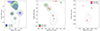 |
Fig. A.1. Pairwise image alignment based on same-UV-range modelfit models. Dash-line circles indicate the pairs of cross-identified components that were used to derive the image shift. Left to right: 15-43 GHz. 43-86 GHz, and 86-227 GHz. In each image, contours represent total intensity at the higher frequency. |
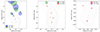 |
Fig. A.2. Best modelfit models after aligning the images. Left to right: 15-43 GHz. 43-86 GHz, and 86-227 GHz. The last pair represents the same model, as that shown in Fig. A1, but with intensity contours from the lower frequency. |
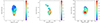 |
Fig. A.3. Pairwise spectral index maps. Left to right: 15-43 GHz. 43-86 GHz, and 86-227 GHz. Contours indicate total intensity at the higher frequency while colors represent spectral index α, defined as Sν ∝ να. |
Appendix B: Data interpolation using modelfit models
When going to higher and higher frequencies, it is more important to work with simultaneous multifrequency data since structural changes in the source might be significant even on a timescale of a week. For NRAO 530, the typical apparent velocity of its moving features is ≈1μas per day. 15 GHz and 43 GHz data were taken during MOJAVE and BU campaigns two months and two weeks apart from the EHT 2017 observations respectively. Structural changes are detectable but modelfit model taken before and after the EHT campaign look similar, see Fig. B1. Therefore, we have taken the components identified in both observations and, for each pair of components, linearly interpolated their parameters to a given date, Apr 4, 2017 in this case. Since we were using only circular Gaussian components and δ-functions, we have only interpolated flux density, position, and size of components.
We have conducted a test to estimate the level of uncertainty introduced by the interpolation procedure. Namely, we have compared the difference between the observed parameters of model components for a given observation with those obtained by interpolation between adjacent epochs. Specifically, we have taken all published models for NRAO 530 at 43 GHz (Weaver et al. 2022) for many epochs. All data were organized into triplets of consecutive models. The first and the last models were used to make an interpolated model for the middle epoch which was compared to the real observed one.
For the comparison we have cross-identified model components between the real and the interpolated models and used only close pairs of components, lying within 20% of their size from each other. The core components were used to align models and hence were excluded from this analysis. Resulting distributions in Fig. B2 show that the mean interpolated values for component positions are close to zero and standard deviation is on the order of 35 μas. This value is comparable to the uncertainty in component position for most of model components in each observation. We also have not found any strong degradation of the interpolation accuracy with the time difference between the epochs used for interpolation.
As noted in Sect. 2, reduced χ2 of these modelfit models is close to that of the CLEAN models. Therefore we self-calibrated the data for epoch 2017 Mar 19 to the interpolated model. This approach allowed us to use image-specific analysis, like producing spectral index maps, using interpolated simultaneous data and keeping data errors taken from real a observation. The same procedure was applied to both 15 GHz and 43 GHz data.
According to the kinematic studies (Lister et al. 2021; Weaver et al. 2022), no new jet component was ejected in 2017. Assuming the structural changes are small at 15 and 43 GHz in the time span of a few months, the interpolation is justified and resultant RM maps are reliable. In Fig. B3 we plot the original 15 and 43 GHz images at available epochs (See Table 1) together with the interpolated images.
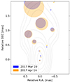 |
Fig. B.1. NRAO 530 43 GHz models for observations taken on 19 Mar and 16 Apr, 2017. The structure consists of the same number of components and these components are easy to cross-identify. |
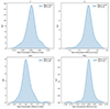 |
Fig. B.2. Probability density function for the difference between the real parameters of the model components and the interpolated values. Top row: component position in R.A.(x) and DEC(y) directions. Bottom row: size and flux density differences. X, Y, and size difference is measured in mas, while flux density difference is measured in Jy. |
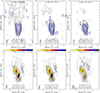 |
Fig. B.3. (top row) 15 GHz polarimetric images obtained on 2017-01-03 (left) and 2017-05-25 (right), and the interpolated one for the epoch of the EHT observations (middle). (bottom row) 43 GHz polarimetric images obtained on 2017-03-19 (left) and 2017-04-16 (right), and the interpolated one for the epoch of the EHT observations (middle). Natural weighting. Total and polarized intensity contours and EVPAs are plotted. Synthesized beams (shaded ellipse) and image parameters (in mJy/beam) are given. |
Appendix C: Model components
In Table C.1 we list all model components at all frequencies used in the paper: 15, 22, 43, 86, and 227 GHz. These models provide a good fit to the data with χ2 comparable to that of CLEAN. At 227 GHz the naming of components is adopted from Jorstad et al. (2023). The component-specific errors were determined in the image plane following eq. 14-5 from Fomalont (1999).
Components of the models at all frequencies
Appendix D: Jet shape based on component sizes
To ensure that the assumptions that we made to use the core-shift method hold, we have checked the shape of the one-epoch jet (the one shown in Fig. 1). We analyzed how the size of individual components depends on their separation from the jet beginning. In Fig. D1, we show the measurements and a linear fit. Before fitting, some outliers were removed, namely, unresolved components and those located beyond 10 mas. Linear fit describes the data in the innermost 2 mas quite well, which means that a conical shape of the jet is a valid assumption. The fit yields the jet apparent opening angle  . The value ϕapp = 10° (ϕint = 0.5°) measured by Pushkarev et al. (2009) falls within our uncertainties and we used it in our calculations.
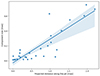 |
Fig. D.1. Size of components at all frequencies depending on their angular separation from the apparent jet beginning at 227 GHz. The line and the shaded area show the best linear fit to the data and the estimate of uncertainty. This dependency reflects the shape of the one-epoch jet. |
Appendix E: Geometry-induced Doppler factor variations
With the model of a precessing jet that we built in Sec.4, we can estimate the impact of the varying viewing angle on the Doppler-boosting factor in the region rdeproj < 5 pc, where apparent cores at different frequencies are located. Fig. E1 shows how the viewing angle θ changes along the jet, as predicted by the fit precession model. It is clear, that for the region of interest, the jet is turning farther away from the observer. While it can increase the path length through the thermal plasma surrounding the jet and hence increase the absolute value of the Faraday RM, the impact on the Doppler factor is negligible for the jet bulk Lorenz factors Γ < 15. We note, that Γ = 15 might be required to explain the rise of the brightness temperature along the jet in this region, but further downstream Γ = 9 is estimated.
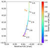 |
Fig. E.1. Zoom into the central region of the NRAO 530. Orange dots show position of the apparent cores at different frequencies. The line shows the precession model and is colored according to the local viewing angle. Several values are marked for convenience. |
Appendix F: Component trajectories
Figure F1 shows trajectories of all model components in NRAO 530 at 43 GHz. The measurements were taken between 2007 and 2018 by Weaver et al. (2022). Trajectories of components in the innermost 1 mas from the core show straight trajectories which is consistent with the precession model for the jet position angle variations.
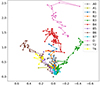 |
Fig. F.1. Trajectories of all model components at 43 GHz covering a period from 2007 to 2018. Plotted based on the data from Weaver et al. (2022). |
All Tables
All Figures
|
Fig. 1. 2D Gaussian best-fit models of NRAO 530 at five frequencies, after alignment. Each resolved Gaussian component is shown as a circle with a diameter of the FWHM of the component. Unresolved components are shown as crosses. Different colors correspond to different frequencies in the dataset, as is shown in the legend. Gray contours represent the source structure at 43 GHz convolved with a circular beam. Horizontal arrows indicate the position of the apparent jet beginning at 227 and 86 GHz, 43 GHz, and 15 and 22 GHz (bottom to top). |
| In the text | |
|
Fig. 2. Apparent core position as a function of frequency. Circles represent data from this research. The measurement at 8 GHz (square) was taken from Pushkarev et al. (2012) and was not used in the fit. The blue curve indicates the best fit of the form r = aν−1/kr + b using 227 GHz as the reference frequency. The orange curve represents the fit adopting the power law index kr = 1. The error bars include component position uncertainty as well as interpolation uncertainty at 15 and 43 GHz. R227 → BH is the angular distance between the 227 GHz core and the central BH. |
| In the text | |
|
Fig. 3. Spectra of the core regions at 15, 43 GHz, and 86 GHz. |
| In the text | |
|
Fig. 4. NRAO 530 jet stack intensity CLEAN image at 43 GHz, with positions of the Gaussian modelfit components overlaid by the precession model (black curve) and the KH instability model (pink curve). All image model components are displayed here as same-size circles for clarity. The colors correspond to frequencies 15, 22, 43, 86, and 227 GHz, as in Fig. 1. The stacked 43 GHz intensity map is presented here with contours at increasing powers of 2, starting from 3 mJy/beam. The map peak is 1.6 Jy/beam. The CLEAN beam is shown in the lower left corner as a 0.25 mas circle. The stacked map was made using component-based method alignment within 14 years (60 epochs) of observations by the BU Blazar program. |
| In the text | |
|
Fig. 5. Observed brightness temperature of model components as a function of the position along the jet, de-projected. Colors represent different frequencies. |
| In the text | |
|
Fig. 6. Total intensity and linear polarization 15, 43, 86, and 227 GHz CLEAN images. Color denotes the distribution of the fractional linear polarization overlaid with the sticks indicating the electric polarization vector directions, not corrected for Faraday rotation. A synthesized beam is shown by a shaded ellipse in the lower left corner and its size is given. The Stokes I contours are plotted at increasing powers of 4, starting from the corresponding 3 rms level. The P contours are drawn at a 4 rms level. Here, we plot interpolated 15 and 43 GHz images (see Sect. 2.6 for details). The original MOJAVE and BU-BLAZAR images are given in Appendix B. |
| In the text | |
|
Fig. 7. Faraday RM at low frequencies. (Top panel) 15−43 GHz RM map with 43 GHz total intensity contours at increasing powers of 2, lowest contour 1.40 mJy beam−1. Sticks denote linear polarization orientation at 43 GHz corrected for Faraday rotation. Numbers indicate locations where the EVPA(λ2)-fits (bottom panel) are taken. Faraday rotation regression is shown by lines, and estimated values are given in rad m−1. |
| In the text | |
|
Fig. 8. Faraday RM at high frequencies. (Top panel) 43−227 GHz rotation measure map with 86 GHz total intensity contours at increasing powers of 2, lowest contour 3.34 mJy beam−1. Sticks denote linear polarization orientation at 86 GHz corrected for Faraday rotation. Numbers indicate locations where the EVPA(λ2) fits (bottom panel) are taken. Faraday rotation regression is shown by lines, and estimated values are given in rad m−1. |
| In the text | |
|
Fig. 9. Map of χ2 values of the EVPA-λ2 fit for the frequency range 43−227 GHz. Gray contours are the same as in Fig. 8. |
| In the text | |
|
Fig. 10. Transverse slice taken across the RM map (Fig. 7) at 1.1 mas. The black dots show the RM fit at every pixel across the slice, with the gray area indicating the error in the fit for each point. |
| In the text | |
|
Fig. 11. Central region of NRAO 530. Contours represent total intensity at 227 GHz. Model components at 227 GHz are named according to Jorstad et al. (2023), at other frequencies – according to Table C.1. The size of Gaussian components is reduced by a factor of five with respect to Fig. 1 for visual clarity. Dashed circles show the location of the apparent VLBI core at different frequencies according to the labels. Component C2 spatially coincides with the apparent core of the 43 GHz model Q0 and an 86 GHz component W1. A weak component, C0b, spatially coincides with the true jet origin calculated using core shift. |
| In the text | |
|
Fig. A.1. Pairwise image alignment based on same-UV-range modelfit models. Dash-line circles indicate the pairs of cross-identified components that were used to derive the image shift. Left to right: 15-43 GHz. 43-86 GHz, and 86-227 GHz. In each image, contours represent total intensity at the higher frequency. |
| In the text | |
|
Fig. A.2. Best modelfit models after aligning the images. Left to right: 15-43 GHz. 43-86 GHz, and 86-227 GHz. The last pair represents the same model, as that shown in Fig. A1, but with intensity contours from the lower frequency. |
| In the text | |
|
Fig. A.3. Pairwise spectral index maps. Left to right: 15-43 GHz. 43-86 GHz, and 86-227 GHz. Contours indicate total intensity at the higher frequency while colors represent spectral index α, defined as Sν ∝ να. |
| In the text | |
|
Fig. B.1. NRAO 530 43 GHz models for observations taken on 19 Mar and 16 Apr, 2017. The structure consists of the same number of components and these components are easy to cross-identify. |
| In the text | |
|
Fig. B.2. Probability density function for the difference between the real parameters of the model components and the interpolated values. Top row: component position in R.A.(x) and DEC(y) directions. Bottom row: size and flux density differences. X, Y, and size difference is measured in mas, while flux density difference is measured in Jy. |
| In the text | |
|
Fig. B.3. (top row) 15 GHz polarimetric images obtained on 2017-01-03 (left) and 2017-05-25 (right), and the interpolated one for the epoch of the EHT observations (middle). (bottom row) 43 GHz polarimetric images obtained on 2017-03-19 (left) and 2017-04-16 (right), and the interpolated one for the epoch of the EHT observations (middle). Natural weighting. Total and polarized intensity contours and EVPAs are plotted. Synthesized beams (shaded ellipse) and image parameters (in mJy/beam) are given. |
| In the text | |
|
Fig. D.1. Size of components at all frequencies depending on their angular separation from the apparent jet beginning at 227 GHz. The line and the shaded area show the best linear fit to the data and the estimate of uncertainty. This dependency reflects the shape of the one-epoch jet. |
| In the text | |
|
Fig. E.1. Zoom into the central region of the NRAO 530. Orange dots show position of the apparent cores at different frequencies. The line shows the precession model and is colored according to the local viewing angle. Several values are marked for convenience. |
| In the text | |
|
Fig. F.1. Trajectories of all model components at 43 GHz covering a period from 2007 to 2018. Plotted based on the data from Weaver et al. (2022). |
| In the text | |
Current usage metrics show cumulative count of Article Views (full-text article views including HTML views, PDF and ePub downloads, according to the available data) and Abstracts Views on Vision4Press platform.
Data correspond to usage on the plateform after 2015. The current usage metrics is available 48-96 hours after online publication and is updated daily on week days.
Initial download of the metrics may take a while.