| Issue |
A&A
Volume 695, March 2025
|
|
|---|---|---|
| Article Number | A260 | |
| Number of page(s) | 10 | |
| Section | Extragalactic astronomy | |
| DOI | https://doi.org/10.1051/0004-6361/202453056 | |
| Published online | 25 March 2025 | |
A helical magnetic field in quasar NRAO 150 revealed by Faraday rotation
1
Max Planck Institute for Radio Astronomy (MPIfR), Auf dem Hügel 69, 53121 Bonn, Germany
2
Lebedev Physical Institute of the Russian Academy of Sciences, Leninsky prospekt 53, 119991 Moscow, Russia
3
Instituto de Física, Pontificia Universidad Católica de Valparaíso, Casilla, 4059 Valparaíso, Chile
4
The University of Mississippi, Department of Physics and Astronomy, Oxford, USA
5
Instituto de Astrofísica de Andalucía-CSIC, Glorieta de la Astronomía s/n, E-18008 Granada, Spain
⋆ Corresponding author; jack.david.livingston+This email address is being protected from spambots. You need JavaScript enabled to view it.
Received:
18
November
2024
Accepted:
18
February
2025
Abstract
Context. Active galactic nuclei (AGN) are some of the most luminous and extreme environments in the Universe. The central engines of AGN are believed to be super-massive black-holes (SMBHs) are fed by accretion discs threaded by magnetic fields within a dense magneto-ionic medium.
Aims. We report our findings from polarimetric very-long-baseline interferometry (VLBI) observations of quasar NRAO 150 taken in October 2022 using a combined network of the Very Long Baseline Array (VLBA) and Effelsberg 100-m Radio Telescope. These observations comprise the first co-temporal multi-frequency polarimetric VLBI observations of NRAO 150 at frequencies above 15 GHz.
Methods. We used the new VLBI polarization calibration procedure, GPCAL, with polarization observations of frequencies of 12 GHz, 15 GHz, 24 GHz, and 43 GHz of NRAO 150. From these observations, we were able to measure the Faraday rotation and use it to derive the intrinsic electric vector position angle (EVPA0) for the source. As a complementary measurement, we determined the behavior of polarization as a function of observed frequency.
Results. The polarization from NRAO 150 only comes from the core region, with a peak polarization intensity occurring at 24 GHz. Across the core region of NRAO 150, we see clear gradients in Faraday rotation and EVPA0 values that are aligned with the direction of the jet curving around the core region. We find that for the majority of the polarized region the polarization fraction is greater at higher frequencies, with intrinsic polarization fractions in the core ≈3%.
Conclusions. The Faraday rotation gradients and circular patterns in EVPA0 offer strong evidence to support the presence of a helical+toroidal magnetic field. Furthermore, the presence of low intrinsic polarization fractions indicate that the polarized emission and, hence, the helical+toroidal magnetic field, is present within the innermost jet.
Key words: polarization / galaxies: magnetic fields / quasars: individual: NRAO 150
© The Authors 2025
 Open Access article, published by EDP Sciences, under the terms of the Creative Commons Attribution License (https://creativecommons.org/licenses/by/4.0), which permits unrestricted use, distribution, and reproduction in any medium, provided the original work is properly cited.
This article is published in open access under the Subscribe to Open model.
Open Access funding provided by Max Planck Society.
1. Introduction
NRAO 150 is a highly variable radio loud quasar with a redshift of z = 1.52 (Acosta-Pulido et al. 2010) and reported viewing angles of θ ≈ 8° (Agudo et al. 2007) and θ ≈ 0.28° (Homan et al. 2021). The source has an apparent jet opening angle of 19.4° (Pushkarev et al. 2017), along with a maximum recorded jet speed of β = 8.65 (Homan et al. 2021) based on the maximum measured jet speed over 42 epochs at 15 GHz, and a variability Doppler factor of δvar = 13.1 (Hovatta et al. 2009). Agudo et al. (2007) found that the inner jet of NRAO 150 swings at ≈6° −11° on a timescale of one year using five epochs at 43 and 86 GHz.
The polarization properties of NRAO 150 were studied by Molina et al. (2014) using observations at 8, 15, 22, 43, and 86 GHz with the Very Long Baseline Array (VLBA) and Global Millimeter VLBI Array (GMVA) from 2006 to 2009. A follow-up study was conducted using additional 2008–2009 observations at 22, 43, and 86 GHz with the VLBA and GMVA (Molina et al. 2016). These studies found that the electric vector polarization angle (EVPA) of the source showed a circular pattern, which they concluded was evidence of a magnetic field with helical+toroidal geometry.
Paraschos et al. (2024) used European VLBI Network (EVN) polarimetric data of NRAO 150 at 22 GHz to calibrate their 3C 84 data. These NRAO 150 data will be presented in Debbrecht et al. in prep. The EVPA they found shows a circular pattern in the core (similar to that found by Molina et al. 2016) and EVPA values aligned with the direction of the bulk jet flow further downstream. Within the core they measured polarization intensities peaking at ∼23 mJy/beam.
When polarized emission passes through a magneto-ionic medium, the EVPA is expected to rotate via birefringence. This effect is called “Faraday rotation” and it is proportional to the square of the observed wavelength. Typically, we assume that this medium or “screen” is external to the polarized emission region. We quantify the amount of Faraday rotation as the observed rotation measure, RMobs, which is characterized as EVPA = EVPA0 + RMobsλ2. Here, EVPA0 is the Faraday corrected or “intrinsic” EVPA at the source.
Next, RM relates to the electron number density, ne, in units of cm−3, and the line-of-sight (LoS) magnetic field, B|| as,
 (1)
(1)
Here, d is the distance to the Faraday rotating medium in pc, dr is the incremental displacement along the LoS measured in pc from the observer to the source, and 𝒞 is a conversion constant, 𝒞 = 0.812 rad m−2 pc−1 cm3 μG−1 (Ferrière et al. 2021). We adopted the vector orientation and sign convention for Faraday rotation according to the procedure outlined by Ferrière et al. (2021).
The Faraday rotation of NRAO 150 was previously measured by Zavala & Taylor (2004), observed in 2001, and as part of a follow-up analysis of the data by Gabuzda et al. (2015). First, Zavala & Taylor (2004) found the majority of Faraday rotation to occur near the optically thick core region and found hints of Faraday rotation that appeared to break the λ2 relation. Gabuzda et al. (2015) re-examined the data from Zavala & Taylor (2004) and found a prominent gradient in Faraday rotation across the core region with a significance of 4.2σ; they concluded such a significant gradient was evidence for a helical+toroidal magnetic field. NRAO 150 is a highly variable source; however, since the 2001 observation from Zavala & Taylor (2004), there has been no new work on the Faraday rotation of NRAO 150. Our work presents the first new Faraday rotation analysis for NRAO 150 in two decades and also offers a higher frequency range than previously covered, allowing us to better understand the magnetic fields of the source closer to the central engine.
For this work, we assume H0 = 71 km s−1 Mpc−1, Ωm = 0.27, and ΩΛ = 0.73 (Komatsu et al. 2009). This corresponds to a luminosity distance for NRAO 150 of 11 193.4 Mpc, with a projected angular scale of 8.55 pc mas−1. Due to the variation in the viewing angles for this source (0.28° or 8°)1 we have kept all physical distances as projected distances.
2. Observations and methods
NRAO 150 was observed on October 1, 2022, using the VLBA and the Effelsberg 100m Radio Telescope (EF) as a joint VLBI network, at central frequencies of 12.168, 15.368, 23.568, and 43.169 GHz, each split into eight intermediate frequencies or IF windows. This observation also included the sources 3C 111, 3C 120, and NGC 1052, as well as a complementary observation of 2023+335, 3C 371, 3C 418, BL Lac, and Cygnus-A on October 2, 2022. Eight out of ten VLBA antennas were available for this observation (BR, FD, LA, NL, OV, SC, MK, and HN).
2.1. A priori and self-calibration
As NRAO 150 is a very bright and compact AGN with typical VLBI peak flux densities exceeding 5 Jy beam−1, it was used as a calibrator source in a priori calibration using the standard procedures described in the AIPS cookbook2 to test for this flux density loss.
After a priori calibration, we found a lower overall flux density for all sources within our observations compared to MOJAVE at 15 GHz (Lister et al. 2018) and Boston BEAM-ME 43 GHz (Jorstad & Marscher 2016) measurements of shared sources. We also performed a-priori calibration following using the rPicard/CASA v7.8.13 pipeline (Janssen et al. 2019). We found that the AIPS a-priori calibrated data shows an overall higher amplitude by 9% than the data processed with rPicard/CASA. A flux density difference of ∼10% has been seen in preliminary analysis conducted by the MOJAVE team comparing rPicard/CASA and AIPS; this is currently being investigated. It is worth noting that according to the NRAO, flux density calibration with the VLBA is only valid to an allowance of ± ∼ 10%4, and we note that the difference of 9% we see is within that margin. Technical issues as well as weather present challenges for an accurate VLBI amplitude calibration. Overall amplitude depends on how bandpass solutions are re-normalized affecting the final values (VLBA Scientific Memo 405). For this reason, MOJAVE uses OVRO (Richards et al. 2011) and BEAM-ME uses Metsahovi single dish data6 to calibrate the flux density scale.
Even accounting for this flux density uncertainty we find additional losses in both the AIPS and rPicard/CASA calibrated data as compared to MOJAVE and BEAM-ME data. This flux density loss comes from erroneous correlation of the VLBA+EF network which is independent of the flux density difference seen between AIPS and rPicard/CASA pipelines. This error occurred due to a mismatch between the EF and VLBA frequency setups which was not accounted for in the correlation. This has been confirmed with the operator of EF. This effect remains if we completely flag EF, as such we require a correction to our absolute amplitude based on external data.
We elected to correct our AIPS calibrated data, to access an overall better dynamic range. We also discovered an issue with rPicard/CASA polarization calibration, which produces a 45° EVPA offset in our observation due to flipping Stokes Q and U. To correct for the overall reduction in flux density due to erroneous correlation of the VLBA+EF network, we used TPOL0003 VLA observations of NRAO 150 using the Very Large Array (VLA) conducted on October 10, 2022, across similar frequency bands as our data. We calibrated these observations using the standard VLA CASA calibration pipeline. We then generated images of the calibrated data of NRAO 150 and compared the derived flux density of the VLA images with the flux density of our VLBA+EF images, finding the multiplicative gain factor that needed correcting. These gain corrections are shown in Table 1.
Observed bands, values used throughout the data calibration, and peak Stokes I and linear polarization intensities.
We performed an amplitude and phase self-calibration on NRAO 150 for all frequencies down to 30 s solution intervals. The gains of EF were considerably lower than expected for the 15 and 24 GHz bands, which was seen for all sources within our observation. As such, we used the VLBA antennas to anchor the gains of EF before proceeding with amplitude self-calibration to preserve the absolute amplitude of the source.
2.2. Polarization calibration
Between a priori and absolute EVPA calibration, we used GPCAL7 (Park et al. 2021) to solve for polarization leakage or “D-terms”. For the leakage calibration we selected NRAO 150, 3C 111, and 3C 120 as calibrators, using an iterative self-calibration approach for ten repeated iterations.
Absolute EVPA calibration was done by “anchoring” to an external observation. We used the TPOL0003 VLA observations of NRAO 150. Polarization calibration was done following the methods outlined in the VLA CASA polarization calibration tutorial8. We created a point source model of EVPA for the source from 12 to 43 GHz and calculated the EVPA offset between the VLA and the integrated EVPA from our D-term corrected VLBA+EF data of NRAO 150 data for each IF window of each band.
2.3. Imaging and error estimation
The images of Stokes I, Q, and U were generated using the entropy stopping criteria imaging script as outlined by Homan et al. (2024). The script is based on the VLBI imaging software Difmap (Shepherd 1997), and images the data using a variety of visibility weightings – specifically, 10 (ultra-uniform), 2 (uniform), and 0 (natural), to catch any residual structure left in the data. To generate the images shown in this work, we used a common resolving element (“restoring beam”) across all frequencies with a major axis of 0.53 mas, a minor axis of 0.35 mas, and a position angle of −22.4°. In Figure 1 we present the generated linear polarization images and Stokes I contours for each observed frequency.
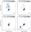 |
Fig. 1. Panels (1) to (4) show the Stokes I contours and linear polarization intensity (shown in gray-scale) of NRAO 150 for 12 (1), 15 (2), 24 (3), and 43 GHz (4). The purple ellipse in panel (4) shows the restoring beam used for all four frequencies. The contours start at 5σI up to the peak increasing by a factor of 2. The blue ticks in panels (1) to (4) show the average EVPA across a 5 × 5 pixel region for each frequency. |
We estimated the Stokes I uncertainty, σI, by finding the root-mean-squared (rms) noise of a 300 × 300 pixel region sufficiently far away from Stokes I emission of the source. We further estimated the error introduced from residual D-terms (σdterm) to the polarized visibilities after calibration using the same approach as shown in Eq. (B4) in Hovatta et al. (2012), finding the median scatter of D-terms for each frequency band, and accounting for six scans of NRAO 150, eight spectral windows, and between seven9 to eight antennas. The scatter of D-terms are shown in Table 1.
The uncertainty of the polarized signal was determined by finding the rms of a 300 × 300 square pixel area away from the source of the Stokes Q and U images (σrms) and combining this uncertainty estimate with that from the σdterm, following equation B5 of Hovatta et al. (2012). The uncertainty of the polarization data (σp) is the combination of the uncertainties from Stokes Q and U, such that  .
.
To estimate the uncertainty of our EVPA measurements, we take the uncertainty assumed from σP, which is σEVPA = σP/(2P), and add an additional error based on the scatter of the VLA data around the model of EVPA used for absolute EVPA calibration. This scatter of the EVPA values are shown in Table 1.
For image alignment between observed frequencies, we implemented a 2D cross-correlation approach on optically thin Stokes I emission similar to that outlined by Molina et al. (2014). We used the Python package phase_cross_correlation from skimage.registration10, but we found that the overall displacement is consistent with zero across all frequencies. As Hovatta et al. (2012) showed that RM is robust against a small misalignment between frequencies up to 0.15 mas for the VLBA at 15 GHz, we do not expect image alignment errors to affect our work.
2.4. Faraday rotation
Following Sarala & Jain (2001), we used a circular statistics approach to fitting RMobs with a fit minimization parameter, χcirc2, defined as:
![Mathematical equation: $$ \begin{aligned} \chi ^2_{\mathrm{circ}} = \sum ^{n_{\nu }}_{i} \frac{1-\cos \left(2 \left[\mathrm{EVPA} - \mathrm{RM}_{\rm obs} \lambda ^2 - \mathrm{EVPA}_{0}\right]\right)}{1-\cos \left(2 \sigma _{\mathrm{EVPA}}\right)}. \end{aligned} $$](/articles/aa/full_html/2025/03/aa53056-24/aa53056-24-eq7.gif) (2)
(2)
Here, nν is the number of frequencies we have polarization information for. By minimizing Eq. (2) we are able to solve for EVPA0 (Sarala & Jain 2001),
![Mathematical equation: $$ \begin{aligned} \mathrm{EVPA}_{0} = \frac{1}{2} \arctan \left(\frac{\sum _i^n (\sin (E)/[1-\cos (2\sigma _{\mathrm{EVPA}})])}{\sum _i^n (\cos (E)/[1-\cos (2\sigma _{\mathrm{EVPA}})])}\right), \end{aligned} $$](/articles/aa/full_html/2025/03/aa53056-24/aa53056-24-eq8.gif) (3)
(3)
where E = 2(EVPA − RMobsλ2). In this formulation, we only require RMobs to model EVPA, without needing to fit the EVPA0 directly, reducing the number of fitted parameters.
We model RMobs for all pixels with a polarized signal greater than 3σP and 5σI for at least two frequencies. For pixels with polarization information for more than two frequencies we reject any fits for which the χcirc2 of the fit exceeds the 95% confidence limit. For these pixels, they may have non-λ2 dependent Faraday rotation, which occurs when there are complex Faraday rotation effects present (Hovatta et al. 2012).
When we measure RMobs in the direction of an extra-galactic source, we are measuring a combination of different contributions to the overall Faraday rotation, such that
 (4)
(4)
Here, RMint is the intrinsic Faraday rotation of the source which needs to be corrected for the redshift, z; RMIGM and RMMW are the intergalactic medium (IGM) and the Milky Way (MW) contributions to RMobs. The magnitude of RMIGM is typically between 1 and 10 rad m−2 (O’Sullivan et al. 2017) and, as such, we ignore the contribution of RMIGM. We estimate RMMW using the RM catalog of Van Eck et al. (2023) taking the median RM of a 2° area around the phase center of NRAO 150, which is RMMW = 52 rad m−2 with a standard deviation of 65 rad m−2.
2.5. Depolarization
Measuring depolarization as a function of frequency can help determine where the RMint originates within the source. We modeled the depolarization following the method outlined by Hovatta et al. (2012),
 (5)
(5)
Here m is the measured polarization degree (as a percentage), m0 is the intrinsic degree of polarization at λ = 0, and b is the depolarization in units of m−4.
There are two main causes of depolarization we consider here: external and internal Faraday dispersion. If there is magneto-ionic turbulence within an external medium, this causes an EVPA de-coherence across the size of the beam, which results in a reduction in the overall linear polarization fraction. This depolarization increases with the observed wavelength, as the size of the resolving beam increases and the variation in RMint is more prominent for greater values of λ2.
For internal Faraday dispersion, we assume that the polarized emission is co-spatial with the Faraday rotating medium. Emission from the source undergoes differential Faraday rotation, depending on where in the medium the emission is generated, which can cause a de-coherence of EVPA and subsequent depolarization.
Depending on the morphology of the emission region, it is also possible to re-align EVPA values, causing “inverse” depolarization (Homan 2012). If we see positive values of b, this indicates the presence of inverse depolarization, which is suggestive of internal Faraday dispersion. The internal Faraday dispersion effect is dependent on the magnitude of RM, such that b ∼ 2RM2. If |b|/(2 RM2) ≤ 1, especially when the magnitude of RM is large, we expect the depolarization observed to be attributed to co-spatial polarized emission and Faraday rotation (Hovatta et al. 2012). If we see large negative values of b that are larger in magnitude than 2 × RM2, this suggests that the depolarization comes from external Faraday dispersion resulting from random fluctuations in RM causing EVPA de-coherence.
3. Results and discussion
In this section, we discuss the linear polarization, Faraday rotation, EVPA0, and depolarization properties of NRAO 150, with an aim to understand the geometry of its magnetic field.
3.1. Linear polarization
In panels (1) to (4) of Fig. 1, we show the linear polarization intensity maps for the four frequency bands in conjunction with Stokes I contours. From these maps we can see that the linear polarization is present near the VLBI “core” position of the source, with a some log magnitude polarized emission extending outwards towards the jet for the 12 and 15 GHz maps. The peak polarization is greatest at 24 GHz, decreasing from 225 mJy beam−1 to 181 mJy beam−1 at 43 GHz, shown in Table 1. Molina et al. (2014) found, for a number of epochs of 22 and 43 GHz, similar linear polarization intensity, as shown in panels (3) and (4). Paraschos et al. (2024), shows considerably lower peak polarization intensity at ∼22 GHz than in our findings (∼23 mJy beam−1 compared to 225 mJy beam−1). This discrepancy may come from the fact that the source is intrinsically variable (also supported by the finding that the peak Stokes I reported in Paraschos et al. 2024 is 2.5 Jy beam−1).
In panels (1) to (4) of Fig. 2, we show the fractional linear polarization for each frequency. We can see that the fractional linear polarization is greater throughout the 12 GHz map, with sections of the jet exceeding 20%, while the fraction near the core is around ∼5%. For panels (2) to (4) we can see that the fractional polarization does not exceed ∼10% in the core. We expect polarization of optically thick regions to not exceed 10–15% and within these regions EVPA runs parallel to the projection of the magnetic field on the plane-of-sky, B⊥ (Pacholczyk 1970). Molina et al. (2014) found fractional polarization of ≈5%,10%,15% for 15, 22, and 43 GHz observations, respectively. Furthermore, Molina et al. (2016) found a fractional polarization of ≈14% around the northern edge of the central region of the source for both frequencies.
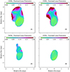 |
Fig. 2. Panels (1) to (4) show the fractional linear polarization for each frequency. The contours are the lowest Stokes I contour levels for all frequencies from Fig. 1. |
3.2. Rotation measure
In Fig. 3, we show the RMint map (corrected for the z of NRAO 150) with ticks showing EVPA0. Most of the RMint of NRAO 150 is negative with the positive peak of RMint = (3.0 ± 0.7)×104 rad m−2 and a negative peak of RMint = ( − 2.0 ± 0.7)×104 rad m−2. Towards the jet, there is a gradient in RMint. In Fig. 4, we show the observed EVPA against λ2 for the three pixels marked by numbers 1, 2, and 3 in Fig. 3. For the pixels, the observed EVPA values fit well to the model for RMobs.
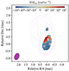 |
Fig. 3. Map of RMint and EVPA0. The tick markers show the average EVPA0 across a 3 × 3 pixel region. The contours are the lowest Stokes I contour levels for all frequencies from Fig. 1. The observed EVPA against λ2 for the three pixels marked by numbers 1,2 and 3 are plotted in Fig. 4. The purple ellipse in panel shows the restoring beam used for all four frequencies. |
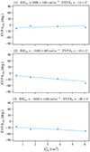 |
Fig. 4. Observed EVPA against λ2 for the three pixels marked by numbers 1, 2, and 3 in Fig. 3. Above each plot is the RMint (corrected for redshift and foreground contribution as discussed in Sect. 2.4) and EVPA0 for that pixel. |
The EVPA0 values shown in Fig. 3 run towards the direction of the jet, gradually bending around the core. We also note that the EVPA0 values run perpendicular to the gradient in RMint in the north of the core. In the optically thick regions of a source, we expect EVPA0 to be aligned with B⊥; the alignment of EVPA0 is suggestive of a B⊥ pointing in the direction of the jet curving around the core region. Both Molina et al. (2014) and Molina et al. (2016) found a similar circular geometry of EVPA for NRAO 150; however, this was not Faraday rotation-corrected.
3.3. Depolarization and maximum polarization
In Fig. 5, we show the map of redshift-corrected bint. Here, bint is the depolarization constant b (discussed in Sect. 2.5) scaled by (1 + z)2 to account for the redshift of NRAO 150. Most of the core region has highly negative values of bint, which reflects depolarization that increases as a function of increasing observed λ.
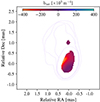 |
Fig. 5. Map of intrinsic depolarization (bint). The contours are the lowest Stokes I contour levels for all frequencies from Fig. 1. |
In Fig. 6, we show the intrinsic polarization degree, m0. Across the entire region, m0 is around 3%, with an increase to 6% on the northern side of the core region. In the small emission we see further down the jet the m0 increases to ≥10%. This preferential increase in polarization degree is similar to that seen in the fractional linear polarization maps (Fig. 2), and the findings of Molina et al. (2014) and Molina et al. (2016). Values of m0 around a few percent hint that the emission we are probing is likely to be optically thick, for which we would expect a lower fractional polarization (Pacholczyk 1970).
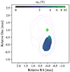 |
Fig. 6. Map of intrinsic polarization degree (m0). The contours are the lowest Stokes I contour levels for all frequencies from Fig. 1. |
In the map of ratios of bint/(2 RMint2) shown in Fig. 7, we see that 31% of pixels have ratios greater than –1, indicating that the majority of pixels show bint/(2 RMint2) < −1. The pixels with negative ratio values are spatially close to the point at which the gradient seen in Fig. 3 passes through zero. We can see that the ratio of bint/(2 RMint2) decreases in magnitude away from this transition going towards bint/(2 RMint2) > −1. Ratios ≥ − 1 indicate that the depolarization we see is explainable by the magnitude of RM causing internal Faraday rotation, without needing to invoke magneto-ionic turbulence as is required in the external Faraday dispersion case.
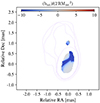 |
Fig. 7. Map of the ratio of bint/(2 RMint2). Grey pixels show rejected fits of RM. The contours are the lowest Stokes I contour levels for all frequencies from Fig. 1. |
3.4. Faraday rotation gradients
In Fig. 8 we show the longest north-south (N-S) (panel (1)) shown in panel (2). Taylor & Zavala (2010) first proposed a list of criteria for Faraday rotation gradients to be considered significant. This was followed up by Hovatta et al. (2012), who extensively tested the validity of RMint gradients, finding that if a gradient has a δRM with ≥3σ confidence and is ≥1.4× the beam full-width half-maximum (FWHM) in the direction of the gradient it is significant. The gradient shown in Fig. 8 has a confidence in δRMint of 5.7σ and is 2× the beam FWHM in the direction of the slice at 0.9 mas in length, corresponding to a projected size of ∼7.7 pc.
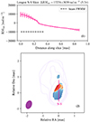 |
Fig. 8. Slice of RMint of NRAO 150 of the longest north-south (N-S) slice (1). Panel (2) is an illustration of slice locations on RM map from Fig. 3. The black dashed line shows the beam full-width half maximum (FWHM) in the direction of the slice. |
Broderick & McKinney (2010) conducted parsec-scale general relativistic magnetohydrodynamic simulations of AGN jets aimed at testing the expected morphology of Faraday rotation. One of their primary findings was that the presence of a significant Faraday rotation gradient indicates the presence of a helical+toroidal magnetic field located within the jet or core of the AGN. This is because foreground clouds, while contributing the overall Faraday rotation of some AGN, should not show Faraday rotation gradients that are correlated with jet structures (Broderick & McKinney 2010).
In their study of Faraday rotation gradients, Gabuzda et al. (2015) found a gradient across the core region of NRAO 150 (observed in 2001 between 8.1 − 15.2 GHz) with a significance of 4.2σ (ΔRMint = 3944 ± 934 rad m−2) and with a length of 1.5 mas. Following the findings of Broderick & McKinney (2010), Gabuzda et al. (2015) concluded that the presence of a significant gradient in the core of NRAO 150 is indicative of the presence of a helical+toroidal magnetic field within the innermost jet of the AGN, even if the region is not optically thin, given the significance and continuity of the RM gradients seen for NRAO 150. We see similar significant and continuous gradients across the core region of NRAO 150. We conclude that the Faraday rotation gradients we see, especially our longest Faraday rotation gradient with ΔRMint = (15 954 ± 2661) rad m−2 across a angular distance of 0.9 mas (∼7.7 pc), indicate a helical+toroidal magnetic field is present within the innermost jet of NRAO 150.
3.5. The magnetic field strength in NRAO 150
In Fig. 8, we see that RMint varies across the source, with a gradient in RMint of ΔRMint = (17 274 ± 3039) rad m−2 with a maximum magnitude value of |RMint|=(9453 ± 2737) rad m−2. This occurs over an apparent size scale of ∼7.7 pc. Assuming an apparent opening angle of 19.4° (Pushkarev et al. 2017) this results in an apparent distance from the jet base of ∼23 pc across the gradient. If we further assume that at 1 pc from the core the free electron number density is between 102 and 104 cm−3 (Lobanov 1998), the magnetic field strength and electron number density both follow as ∼r−1 (Lobanov 1998; Pushkarev et al. 2012; Nokhrina & Pushkarev 2024). Integrating along a path-length of 22 pc, the relationship between RMint and B|| from Eq. (1) becomes
 (6)
(6)
where nr = 1 is the electron density at 1 pc from the core. Setting RMint = (9453 ± 2737) rad m−2 we get a lower limit of B||,0 ∼ 1.2 μG (assuming n0 = 104 cm−3) and an upper limit of B||,0 ∼ 122 μG (n0 = 102 cm−3). This is similar to the LoS magnetic field strength estimate from Hovatta et al. (2019) for 3C 273 of 62 μG, assuming an electron number density of 1000 cm−3 coming from the narrow line region (Zavala & Taylor 2004).
Nokhrina & Pushkarev (2024) used the relationship between core-shift (Lobanov 1998) and the energy equipartition assumption to find that the typical total magnetic field strength at 1 pc from the core of AGN is ∼84 mG. If we instead assume that the LOS magnetic field strength and the plane-of-sky magnetic field strength are the same (i.e. B||,r = 1 ∼ 59 mG), this results in an electron number density of nr = 1 ∼ 2 × 10⁻¹ cm−3. To differentiate between the scenarios of a weak magnetic field (1.2 − 122 μG) and a small electron number density, we plan to conduct simulations in a future publication, similar to those performed by MacDonald & Nishikawa (2021).
4. Summary and conclusions
In this work, we present multi-frequency polarimetric observations of quasar NRAO 150 taken using the VLBA+EF telescopes at 12, 15, 24, and 43 GHz. This work builds on previous studies of the source, with the unique quality of having high-frequency (between 12–43 GHz) polarimetric observations that are quasi-simultaneous. From the linearly polarized emission, we calculated the Faraday rotation, intrinsic electric vector position angle (EVPA0), and depolarization properties of the source.
We find a circular pattern of EVPA0 and the presence of Faraday rotation gradients across the core region of NRAO 150, both of which are consistent with a helical+toroidal magnetic field. The predicted maximum polarization fraction, m0, for this region is ≈3%, consistent with emission from optically thick regions in AGN. Together with the magnitude of Faraday rotation in this region, we conclude that the observed polarized emission is produced within the jet (as opposed to an external medium).
The results of this study, in conjunction with previous findings from Molina et al. (2014), Gabuzda et al. (2015), and Molina et al. (2016), show there is a helical+toroidal magnetic field within the innermost jet region of NRAO 150.
Data availability
The maps of RMobs and EVPA0 shown in Fig. 3 and associated uncertainties are available at the CDS via anonymous ftp to cdsarc.cds.unistra.fr (130.79.128.5) or via https://cdsarc.cds.unistra.fr/viz-bin/cat/J/A+A/695/A260
For θ ≈ 0.28° the de-projected scale is 1749 pc mas−1, whereas θ ≈ 8° results in a scale of 61 pc mas−1.
The FD antenna was not present for the 43 GHz observation.
Acknowledgments
We thank Sebastiano D. von Fellenberg for his helpful comments on the manuscript draft and we thank the anonymized reviewer for their constructive feedback during the review process. M2FINDERS project has received funding from the European Research Council (ERC) under the European Union’s Horizon 2020 research and innovation programme (grant agreement No 101018682). MW is supported by a Ramón y Cajal grant RYC2023-042988-I from the Spanish Ministry of Science and Innovation. The VLBA is an instrument of the National Radio Astronomy Observatory. The National Radio Astronomy Observatory is a facility of the National Science Foundation operated by Associated Universities, Inc. This work made use of the Swinburne University of Technology software correlator (Deller et al. 2011), developed as part of the Australian Major National Research Facilities Programme and operated under licence. This research has made use of data from the MOJAVE database that is maintained by the MOJAVE team (Lister et al. 2018). This study makes use of VLBA data from the VLBA-BU Blazar Monitoring Program (BEAM-ME and VLBA-BU-BLAZAR; http://www.bu.edu/blazars/BEAM-ME.html), funded by NASA through the Fermi Guest Investigator Program. YYK was supported by the MuSES project which has received funding from the European Research Council (ERC) under the European Union’s Horizon 2020 Research and Innovation Programme (grant agreement No 101142396).
References
- Acosta-Pulido, J. A., Agudo, I., Barrena, R., et al. 2010, A&A, 519, A5 [NASA ADS] [CrossRef] [EDP Sciences] [Google Scholar]
- Agudo, I., Bach, U., Krichbaum, T. P., et al. 2007, A&A, 476, L17 [NASA ADS] [CrossRef] [EDP Sciences] [Google Scholar]
- Broderick, A. E., & McKinney, J. C. 2010, ApJ, 725, 750 [Google Scholar]
- Deller, A. T., Brisken, W. F., Phillips, C. J., et al. 2011, PASP, 123, 275 [Google Scholar]
- Ferrière, K., West, J. L., & Jaffe, T. R. 2021, MNRAS, 507, 4968 [Google Scholar]
- Gabuzda, D. C., Knuettel, S., & Reardon, B. 2015, MNRAS, 450, 2441 [CrossRef] [Google Scholar]
- Homan, D. C. 2012, ApJ, 747, L24 [Google Scholar]
- Homan, D. C., Cohen, M. H., Hovatta, T., et al. 2021, ApJ, 923, 67 [NASA ADS] [CrossRef] [Google Scholar]
- Homan, D. C., Roth, J. S., & Pushkarev, A. B. 2024, AJ, 167, 11 [Google Scholar]
- Hovatta, T., Valtaoja, E., Tornikoski, M., & Lähteenmäki, A. 2009, A&A, 494, 527 [CrossRef] [EDP Sciences] [Google Scholar]
- Hovatta, T., Lister, M. L., Aller, M. F., et al. 2012, AJ, 144, 105 [Google Scholar]
- Hovatta, T., O’Sullivan, S., Martí-Vidal, I., Savolainen, T., & Tchekhovskoy, A. 2019, A&A, 623, A111 [NASA ADS] [CrossRef] [EDP Sciences] [Google Scholar]
- Janssen, M., Goddi, C., van Bemmel, I. M., et al. 2019, A&A, 626, A75 [NASA ADS] [CrossRef] [EDP Sciences] [Google Scholar]
- Jorstad, S., & Marscher, A. 2016, Galaxies, 4, 47 [Google Scholar]
- Komatsu, E., Dunkley, J., Nolta, M. R., et al. 2009, ApJS, 180, 330 [NASA ADS] [CrossRef] [Google Scholar]
- Lister, M. L., Aller, M. F., Aller, H. D., et al. 2018, ApJS, 234, 12 [CrossRef] [Google Scholar]
- Lobanov, A. P. 1998, A&A, 330, 79 [NASA ADS] [Google Scholar]
- MacDonald, N. R., & Nishikawa, K. I. 2021, A&A, 653, A10 [Google Scholar]
- Martí-Vidal, I., Mus, A., Janssen, M., de Vicente, P., & González, J. 2021, A&A, 646, A52 [NASA ADS] [CrossRef] [EDP Sciences] [Google Scholar]
- Molina, S. N., Agudo, I., Gómez, J. L., et al. 2014, A&A, 566, A26 [NASA ADS] [CrossRef] [EDP Sciences] [Google Scholar]
- Molina, S. N., Agudo, I., Gómez, J. L., et al. 2016, Galaxies, 4, 70 [NASA ADS] [CrossRef] [Google Scholar]
- Nokhrina, E. E., & Pushkarev, A. B. 2024, MNRAS, 528, 2523 [NASA ADS] [CrossRef] [Google Scholar]
- O’Sullivan, S. P., Purcell, C. R., Anderson, C. S., et al. 2017, MNRAS, 469, 4034 [CrossRef] [Google Scholar]
- Pacholczyk, A. 1970, Radio Astrophysics: Nonthermal Processes in Galactic and Extragalactic Sources, Astronomy and Astrophysics Series (W. H. Freeman) [Google Scholar]
- Paraschos, G. F., Debbrecht, L. C., Kramer, J. A., et al. 2024, A&A, 686, L5 [NASA ADS] [CrossRef] [EDP Sciences] [Google Scholar]
- Park, J., Byun, D.-Y., Asada, K., & Yun, Y. 2021, ApJ, 906, 85 [NASA ADS] [CrossRef] [Google Scholar]
- Pushkarev, A. B., Hovatta, T., Kovalev, Y. Y., et al. 2012, A&A, 545, A113 [NASA ADS] [CrossRef] [EDP Sciences] [Google Scholar]
- Pushkarev, A. B., Kovalev, Y. Y., Lister, M. L., & Savolainen, T. 2017, MNRAS, 468, 4992 [Google Scholar]
- Richards, J. L., Max-Moerbeck, W., Pavlidou, V., et al. 2011, ApJS, 194, 29 [Google Scholar]
- Sarala, S., & Jain, P. 2001, MNRAS, 328, 623 [NASA ADS] [CrossRef] [Google Scholar]
- Shepherd, M. C. 1997, in Astronomical Data Analysis Software and Systems VI, eds. G. Hunt, & H. Payne, ASP Conf. Ser., 125, 77 [Google Scholar]
- Taylor, G. B., & Zavala, R. 2010, ApJ, 722, L183 [NASA ADS] [CrossRef] [Google Scholar]
- Van Eck, C. L., Gaensler, B. M., Hutschenreuter, S., et al. 2023, ApJS, 267, 28 [NASA ADS] [CrossRef] [Google Scholar]
- Zavala, R. T., & Taylor, G. B. 2004, ApJ, 612, 749 [NASA ADS] [CrossRef] [Google Scholar]
Appendix A: Alternative polarization calibration using CASA/PolSolve
As part of this work, the rPicard/CASA calibrated data (discussed in Sect. 2.1) were also polarization leakage-calibrated using PolSolve v211 (Martí-Vidal et al. 2021) and absolute EVPA corrected using CASA function polcal. After D-term and absolute EVPA correction the 15 GHz, 24 GHz, and 43 GHz linear polarization and EVPA maps were similar to those seen in Fig. 1, however we saw significant differences for the 12 GHz band. In Fig. A.1, we show the 12 GHz linear polarization and EVPA distribution using these alternative methods. Compared to the 12 GHz band in Fig. 1, we can see a flip in EVPA values of ∼90° in the core region and a significant difference in overall linear polarization morphology. We also see a much larger polarized intensity with a peak of 520 mJy beam−1.
The D-terms derived by PolSolve took 16 iterations to converge for the 12 GHz band, whereas it took 2, 5, and 4 iterations for the 15 GHz, 24 GHz, and 43 GHz bands, indicating that the polarization leakage was not well characterized for the 12 GHz band. The significant differences in linear polarization of the 12 GHz band using these CASA based methods may be due to a bug we found in the rPicard/CASA pipeline, which flips Stokes Q and U, resulting in a rotation of the EVPA distribution by 45°, an issue with D-term characterization using PolSolve, or the application of CASA function polcal in absolute EVPA calibration for VLBI data. Due to this reason we elected to use GPCAL and AIPS function CLCOR to correct for polarization leakage and perform absolute EVPA correction.
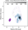 |
Fig. A.1. Stokes I contours and linear polarization intensity (shown in gray-scale) of NRAO 150 for the 12 GHz band derived using a priori calibration from rPicard/CASA, polarization leakage calibration from PolSolve, and absolute EVPA correction using CASA. The purple ellipse shows the restoring beam used. The contours start at 5σI up to the peak of Stokes I increasing by a factor of 2. The blue ticks show the average EVPA across a 5 × 5 pixel region. |
All Tables
Observed bands, values used throughout the data calibration, and peak Stokes I and linear polarization intensities.
All Figures
|
Fig. 1. Panels (1) to (4) show the Stokes I contours and linear polarization intensity (shown in gray-scale) of NRAO 150 for 12 (1), 15 (2), 24 (3), and 43 GHz (4). The purple ellipse in panel (4) shows the restoring beam used for all four frequencies. The contours start at 5σI up to the peak increasing by a factor of 2. The blue ticks in panels (1) to (4) show the average EVPA across a 5 × 5 pixel region for each frequency. |
| In the text | |
|
Fig. 2. Panels (1) to (4) show the fractional linear polarization for each frequency. The contours are the lowest Stokes I contour levels for all frequencies from Fig. 1. |
| In the text | |
|
Fig. 3. Map of RMint and EVPA0. The tick markers show the average EVPA0 across a 3 × 3 pixel region. The contours are the lowest Stokes I contour levels for all frequencies from Fig. 1. The observed EVPA against λ2 for the three pixels marked by numbers 1,2 and 3 are plotted in Fig. 4. The purple ellipse in panel shows the restoring beam used for all four frequencies. |
| In the text | |
|
Fig. 4. Observed EVPA against λ2 for the three pixels marked by numbers 1, 2, and 3 in Fig. 3. Above each plot is the RMint (corrected for redshift and foreground contribution as discussed in Sect. 2.4) and EVPA0 for that pixel. |
| In the text | |
|
Fig. 5. Map of intrinsic depolarization (bint). The contours are the lowest Stokes I contour levels for all frequencies from Fig. 1. |
| In the text | |
|
Fig. 6. Map of intrinsic polarization degree (m0). The contours are the lowest Stokes I contour levels for all frequencies from Fig. 1. |
| In the text | |
|
Fig. 7. Map of the ratio of bint/(2 RMint2). Grey pixels show rejected fits of RM. The contours are the lowest Stokes I contour levels for all frequencies from Fig. 1. |
| In the text | |
|
Fig. 8. Slice of RMint of NRAO 150 of the longest north-south (N-S) slice (1). Panel (2) is an illustration of slice locations on RM map from Fig. 3. The black dashed line shows the beam full-width half maximum (FWHM) in the direction of the slice. |
| In the text | |
|
Fig. A.1. Stokes I contours and linear polarization intensity (shown in gray-scale) of NRAO 150 for the 12 GHz band derived using a priori calibration from rPicard/CASA, polarization leakage calibration from PolSolve, and absolute EVPA correction using CASA. The purple ellipse shows the restoring beam used. The contours start at 5σI up to the peak of Stokes I increasing by a factor of 2. The blue ticks show the average EVPA across a 5 × 5 pixel region. |
| In the text | |
Current usage metrics show cumulative count of Article Views (full-text article views including HTML views, PDF and ePub downloads, according to the available data) and Abstracts Views on Vision4Press platform.
Data correspond to usage on the plateform after 2015. The current usage metrics is available 48-96 hours after online publication and is updated daily on week days.
Initial download of the metrics may take a while.