| Issue |
A&A
Volume 698, June 2025
|
|
|---|---|---|
| Article Number | A210 | |
| Number of page(s) | 10 | |
| Section | Extragalactic astronomy | |
| DOI | https://doi.org/10.1051/0004-6361/202453542 | |
| Published online | 17 June 2025 | |
Helical magnetic field structure in 3C 273
A Faraday rotation analysis using multi-frequency polarimetric VLBA data
1
Instituto de Astrofísica de Andalucía-CSIC, Glorieta de la Astronomía s/n, E-18008 Granada, Spain
2
Korea Astronomy and Space Science Institute, Daedeok-daero 776, Yuseong-gu, Daejeon 34055, Republic of Korea
3
Department of Astronomy, Yonsei University, Yonsei-ro 50, Seodaemun-gu Seoul 03722, Republic of Korea
4
Institut de Radioastronomie Millimétrique, Avenida Divina Pastora, 7m Loca 20, E-18012 Granada, Spain
5
Max-Planck-Institut für Radioastronomie, Auf dem Hügel 69, D-53121 Bonn, Germany
6
Orchideenweg 8, D-53123 Bonn, Germany
⋆ Corresponding author: This email address is being protected from spambots. You need JavaScript enabled to view it.
Received:
20
December
2024
Accepted:
15
April
2025
Abstract
We present a study on rotation measure (RM) of the quasar 3C 273. This analysis aims to discern the magnetic field structure and its temporal evolution. The quasar 3C 273 is one of the most studied active galactic nuclei due to its high brightness, strong polarisation, and proximity, which enables the resolving of the transverse structure of its jet in detail. We used polarised data from 2014, collected at six frequencies (5, 8, 15, 22, 43, 86 GHz) with the Very Long Baseline Array, to produce total and linear polarisation-intensity images, as well as RM maps. Our analysis reveals a well-defined transverse RM gradient across the jet, indicating a helical, ordered magnetic field that threads the jet and likely contributes to its collimation. Furthermore, we identified temporal variations in the RM magnitude when compared with prior observations. These temporal variations show that the environment around the jet is dynamic, with changes in the density and magnetic field strength of the sheath that are possibly caused by interactions with the surrounding medium.
Key words: methods: observational / techniques: interferometric / techniques: polarimetric / galaxies: jets / galaxies: magnetic fields / quasars: general
© The Authors 2025
 Open Access article, published by EDP Sciences, under the terms of the Creative Commons Attribution License (https://creativecommons.org/licenses/by/4.0), which permits unrestricted use, distribution, and reproduction in any medium, provided the original work is properly cited.
This article is published in open access under the Subscribe to Open model. This email address is being protected from spambots. You need JavaScript enabled to view it. to support open access publication.
1. Introduction
Magnetic fields are considered a dominant factor in the launching, acceleration, and collimation of relativistic jets in active galactic nuclei (AGNs) (Blandford et al. 2019). Theoretical models suggest that jet formation is driven either by the extraction of energy from a rotating black hole (the Blandford-Znajek mechanism; Blandford & Znajek 1977) or by magnetic forces acting on material in the accretion disc (the Blandford-Payne mechanism; Blandford & Payne 1982). Both processes require the presence of a structured magnetic field with poloidal (along the jet axis) and toroidal (wrapped around the jet) components. Simulations using general relativistic magnetohydrodynamics (GRMHD) and relativistic magnetohydrodynamics (RMHD) (e.g., Fuentes et al. 2018) have shown that the accretion flow around the black hole naturally develops a “spine-sheath” configuration, which may act as a magnetized boundary layer for the jet (Asada et al. 2008; Gómez et al. 2008, 2012).
Moreover, the Event Horizon Telescope collaboration (EHTC) performed a detailed theoretical study of a jet-producing AGN system based on GRMHD simulations for M 87 (EHTC 2019, 2021), highlighting the role of the Faraday rotation effect in the interpretation of the polarimetric observations of AGNs.
Despite the success of numerical simulations in supporting these models, observational evidence for the detailed structure of the magnetic field, particularly its toroidal component, remains scarce (Zamaninasab et al. 2013; Molina et al. 2014; Pasetto et al. 2021). Observations of linearly polarised synchrotron radiation provide insight into the magnetic field orientation projected on the plane of the sky. The highest resolution linear polarisation maps were obtained from Very Long Baseline Interferometry (VLBI) observations (e.g., Boccardi et al. 2017; Hada 2019; Wielgus et al. 2022; Jorstad et al. 2023), which probe the innermost regions of AGN jets. However, on their own, these polarisation maps cannot fully constrain the three-dimensional (3D) structure of the magnetic field.
To infer the magnetic field component along the line of sight (perpendicular to the plane of the sky), we took Faraday rotation into account. This effect consists of a rotation (dependent on the wavelength) of the polarisation angle of the emission going through a magnetised medium. That is to say, the electric vector position angle (EVPA) is rotated by the (line-of-sight) magnetic field. Thus, the strength and direction of this magnetic field can be inferred through the rotation measure (RM), quantifying this rotation and providing information on the magnetised environment of the jet.
Theoretically, the RM is directly proportional to the line-of-sight magnetic field strength (B||) and the electron density (ne) in the medium, integrated along the path length (dy) (Burn 1966):
 (1)
(1)
where the RM is measured in radians per square metre (rad/m2), B|| is in Gauss, ne is in cm−3, and dy is in parsecs (pc). Thus, by mapping the RM across a jet, we can investigate the magnetic field structure using different features such as gradients. For example, a smooth transverse gradient in a jet, given that the RM is sensitive to the magnetic field direction, would indicate a continuous change in the magnetic field direction, which would evidence the existence of a helical magnetic field (Blandford 1988, 1993; Asada et al. 2002; Gómez et al. 2012, 2016; Pasetto et al. 2021).
In the simplest case, assuming a uniform magnetic field external to the jet (Hovatta et al. 2012), the observed EVPA χobs is related to the intrinsic EVPA χ0 and the square of the observing wavelength (λ2) through the RM as
 (2)
(2)
The quasar 3C 273, at redshift z = 0.158 (Schmidt 1963), is an ideal candidate for RM studies due to its brightness and high polarisation, also showing in many cases a well-resolved jet structure (e.g., Davis et al. 1985; Conway et al. 1993; Jester et al. 2005; Perley & Meisenheimer 2017). Over the years, it has been the subject of numerous VLBI monitoring campaigns aimed at understanding its jet morphology and magnetic field structure (e.g., Krichbaum et al. 1990; Lobanov & Zensus 2001; Savolainen et al. 2006; Kovalev et al. 2016; Bruni et al. 2017; Lister et al. 2019, 2021).
The first detection of a transverse RM gradient in 3C 273 was reported by Asada et al. (2002), suggesting the presence of a toroidal magnetic field. Later studies confirmed this finding (Zavala & Taylor 2005; Asada et al. 2005; Attridge et al. 2005), with similar RM gradients observed in other AGNs (e.g., Gómez et al. 2012; Gabuzda et al. 2017; Kravchenko et al. 2017), further supporting the notion that jets are threaded by helical magnetic fields (e.g., Gómez et al. 2016).
In this paper, we present new multi-frequency VLBI observations of 3C 273, focusing on the study of RM maps to better understand the geometry of the magnetic field structure in this source. We compare our results with previous works, offering new insights into the jet’s magnetic field structure and evolution. The paper is organised as follows. Section 2 describes the observations, data reduction, and calibration procedures. Section 3 presents our results, which are then discussed in detail in Section 4. We also include an appendix featuring the goodness of the fit of the RM maps. Throughout this work, we assumed a cosmology with H0 = 71 km s−1 Mpc−1, Ωm = 0.27, and ΩΛ = 0.73 (Komatsu et al. 2009), where 1 milliarcsecond corresponds to 2.71 pc in projected distance.
2. Observation and data analysis
The observations presented in this work were conducted on 2014, November 21 using the Very Long Baseline Array (VLBA) as part of an astrometric multi-frequency programme (with reference BG216). This programme targeted a sample of BL Lacs, flat-spectrum radio quasars, and radio galaxies. Due to the astrometric nature of the programme, the observing strategy involved alternating scans between the target sources and nearby calibrators at different frequencies. As a result, the scans on the target source were relatively short – typically less than 30 s – a standard approach in astrometric experiments used to maintain high positional accuracy while minimising systematic errors introduced by atmospheric or instrumental effects. This strategy, combined with interleaving scans at multiple frequencies, provided comprehensive uv coverage for the sources.
All ten VLBA antennas were present during the observation, which spanned six frequencies: 4.98, 8.42, 15.25, 21.89, 43.79, and 87.55 GHz. The data were recorded in eight IFs of 32 MHz, amounting to 256 MHz total bandwidth per frequency.
The on-source time ranged from 10 minutes at the lower three frequencies, to 4 h 46 m at 22 GHz, and 47 m at the highest two frequencies. The integration time at 22 GHz is significantly longer because the proposal was originally intended for astrometry, and 22 GHz was used as the reference frequency for regular phase reference and frequency-phase-transfer referencing. A summary of the Fourier coverages can be found in Appendix B.
2.1. Data reduction
The calibration and processing of the data were performed using the National Radio Astronomy Observatory (NRAO) Astronomical Image Processing System (AIPS; Greisen 2003). Standard procedures for polarimetric VLBI observations were followed for phase and amplitude calibration, as described in the AIPS Cookbook1. We applied a priori calibration to the correlated visibility amplitudes using system temperature measurements and gain curves specific to each station. Phase calibration was carried out by performing a fringe-fitting procedure on the data, after correcting for the parallactic angle. Additionally, we corrected for phase bandpass, delay, and rate offsets, which resulted in strong fringe detections across all baselines. The calibrator 4C 39.25 was used as a fringe finder and bandpass calibrator for all frequencies except 86 GHz, for which 3C 273 was used instead.
Subsequent data editing was performed interactively using Difmap software (Shepherd et al. 1994; Shepherd 2011) to remove outliers and poor-quality data, which could introduce noise or artefacts into the imaging process. The final images were produced through iterative CLEAN deconvolution, ensuring that the imaging process accurately reconstructed the brightness distribution of the source while minimising noise.
2.2. Polarisation and rotation measure calculation
The instrumental polarisation calibration (commonly referred to as D-term calibration) was performed using the task LPCAL in AIPS on 3C 273 itself, following the correction for cross-hand delays using the RLDLY task. Once the data are fully calibrated both in intensity and polarisation, to calculate the rotation measure it is necessary to first calibrate the absolute electric vector position angle at each frequency by using single-dish measurements or close-in-time observations from monitoring programmes on our target source, 3C 273.
For 5 and 8 GHz, we used single-dish data from the Monitoring the Stokes Q, U, I and V Emission of AGN jets in Radio (QUIVER) project, obtained with the Effelsberg radio telescope (Myserlis et al. 2018; Angelakis et al. 2019) in the frame of the F-GAMMA monitoring programme. These observations, conducted at 4.85 and 8.35 GHz, were taken ten days after our VLBA session and yielded EVPA values of −28 ± 2° and −36 ± 2°, respectively. For 15 and 43 GHz, we obtained the EVPA correction using archival data from the MOJAVE (Lister et al. 2009) and BEAM-ME (Jorstad et al. 2017) monitoring programmes. We applied the appropriate rotation by comparing our observed EVPAs with these archival values. For 22 GHz, no single-dish measurements were available; hence, to find the appropriate rotation used for the RM map we first corrected 15 and 43 GHz polarisation images, calculated the average EVPA of each map, and then, assuming the linear relation mentioned in Sect. 1, we interpolated the average for the 22 GHz map in order to apply the corresponding rotation. In this way, we provide a reasonable approximation in the absence of direct data.
The RM maps were generated using data from three frequencies at a time, ensuring consistent uv coverage, pixel size, and image resolution across the different frequencies. For an appropriate comparison between frequencies, higher frequency images were convolved with the restoring beam of the lowest frequency. Only regions of polarised intensity with a signal-to-noise ratio greater than 4σ (where sigma is the rms value from Difmap) were used in the analysis. If no polarisation was detected simultaneously at all three frequencies, the corresponding RM pixel was blanked out on the map.
Image alignment across different frequencies was necessary due to the core shift caused by synchrotron self-absorption (Blandford & Königl 1979). We aligned the images using 2D cross-correlation, following the method described by Walker et al. (2000) and Croke & Gabuzda (2008). After cross-correlation, the cumulative shifts for each frequency relative to the reference (highest frequency) were determined and corrected for, finding that they followed an inverse proportionality to the frequency, consistently with the expected trend of a conical Blandford & Königl jet model (Blandford & Königl 1979). Finally, due to the inherent π ambiguity in the EVPAs, π rotations were manually applied to ensure the best fit to the λ2 law in the RM analysis.
The VLBA antennas are not optimised for observations at 86 GHz, resulting in poor sensitivity at this frequency, both in total intensity and polarised flux. Because of this limited sensitivity, the lack of significant polarisation, and the absence of simultaneous single-dish measurements available for calibrating the absolute EVPA, the 86 GHz image was not included in the Faraday rotation analysis.
3. Results
In this section, we present VLBA polarimetric images of 3C 273 at 5, 8, 15, 22, 43, and 86 GHz (Figure 1). The total intensity images are shown with contour lines above the 5σ level, while the EVPAs are overlaid as white ticks. The total polarised intensity is displayed in colour, with only pixels above 4σ included in the polarization map; any pixels below this threshold are blanked out.
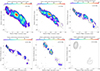 |
Fig. 1. VLBA total and linear polarisation images at different frequencies. Contours show total intensity above a threshold of 5σ; colour scale represents the linearly polarised intensity above 4σ; white ticks indicate the observed electric vector position angle. The peak value of total flux density is 2.83, 2.67, 1.55, 2.08, 3.89, 2.42 Jy/beam for 5, 8, 15, 22, 43, and 86 GHz, respectively. The corresponding rms is 12.55, 4.01, 1.96, 1.23, 2.64, and 5.49 mJy/beam. |
We provide two RM maps derived from observations at 5–8–15 GHz and 15–22–43 GHz, which allowed us to investigate the magnetic field structure across different regions of the jet (Figure 2). Finally, we present images showing transverse sections across the jet at several locations that we used to analyse the asymmetry of the jet in different aspects: the total intensity, the linear polarisation intensity and the degree of polarisation at 5 GHz (Figure 3) and the RM distribution in both RM maps (Figure 4).
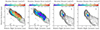 |
Fig. 2. Rotation measure maps of 3C 273 using 5–8–15 GHz (left column, top) and 15–22–43 GHz (left column, bottom) and its respective errors (right column). Corrected (intrinsic) EVPAs are plotted as dark blue ticks. |
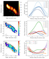 |
Fig. 3. Transversal sections for total intensity image at 5 GHz (top row), linear polarisation at 5 GHz (central row), and degree of polarisation (bottom row). Units are displayed in the left column. The order of the sections along the jet is numbered in the total intensity image. |
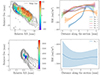 |
Fig. 4. Transversal sections for RM map using 5–8–15 GHz (top row) and 15–22–43 GHz (bottom row). The order and values of the sections are displayed from left to right, as shown in Figure 3. |
3.1. Maps of linear polarization
The total intensity and the polarisation structure in Figure 1 of 3C 273 at different frequencies are consistent with previous observations of 3C 273 (Asada et al. 2002; Zavala & Taylor 2005; Hovatta et al. 2012). As discussed in Section 3.2 (see also Figure 2), the EVPAs are significantly influenced by Faraday rotation, and once corrected, the magnetic field appears to be predominantly toroidal.
The core is located at the northeastern, upstream end of the jet, where linear polarisation is significantly reduced, primarily due to opacity and beam depolarisation effects. At 5 and 8 GHz, a bright, highly polarised component is visible around 10 mas from the core. This feature fades at higher frequencies, although the overall jet structure remains consistent with archival images from the MOJAVE and BEAM-ME programmes. As the core becomes progressively optically thin at 15 and 22 GHz, a new component emerges around 1 mas from the core. Close-in-time MOJAVE observations at 15 GHz and BEAM-ME observations at 43 GHz indicate that this component is moving outward. A comparison with Hada et al. (2016), which used 43 GHz data from February 2014, shows the presence of this component at 1 mas, consisting of two subcomponents referred to as P2 and P3. In our polarisation images taken nine months later, these P2 and P3 components appear to evolve and move further downstream from the core.
We also present one of the few images of 3C 273 at 86 GHz, which is consistent with previous observations by Attridge et al. (2005), Hada et al. (2016), and Hovatta & Lindfors (2019), and more recently by Okino et al. (2022), which incorporated ALMA data for the first time. Although the sensitivity at this high frequency is limited, the total intensity image plotted in contours reveals the core and the brightness structure (component) around 1 mas, which are consistent with lower frequency images. Unfortunately, no significant polarisation is detected at this frequency.
3.2. Rotation measure maps
In this section, we present RM maps in Figure 2 that are derived from two frequency sets, 5–8–15 GHz and 15–22–43 GHz, along with their corresponding error maps. Previous RM studies (Zavala & Taylor 2001; Wardle 2018; Hovatta & Lindfors 2019) typically utilised only two frequencies for a linear fit. By incorporating three frequencies in our analysis, we achieve a more robust and statistically significant estimate of RM. The goodness of the fit of the linear relation is presented in Appendix A, where we use the reduced χ2 as a metric, as in Lisakov et al. (2021), blanking pixels that had χ2 > 5.99 (with 3 data points and 2 degrees of freedom indicates a 95% confidence level). The maps, shown in Figure 2, are overlaid with total intensity contours and the RM-corrected EVPAs. The RM error maps were constructed using the square root of the variance of the parameter estimates from the linear fitting.
For the first RM map, derived from 5–8–15 GHz observations, the values range from approximately −400 rad m−2 to 400 rad m−2, which are consistent in terms of order of magnitude with those reported in previous studies at similar frequencies (Asada et al. 2002, 2008; Hovatta et al. 2012; Lisakov et al. 2021). A clear transverse RM gradient is evident, also presenting a sign change across the jet. That is to say, the different signs at both ends of the gradient are attributed to differences in the line-of-sight magnetic field direction. Thus, it reflects a systematic variation in the magnetized plasma’s properties across the jet, consistent with the geometry and structure expected for a persistent helical magnetic field.
As a byproduct of obtaining the RM maps from a linear approximation, we estimate the intrinsic EVPA of the source (i.e. after correcting for Faraday rotation), which corresponds to the y-intercept of the linear regression. Plotted as dark blue ticks, they follow the jet direction, signalling that the Faraday rotation effect is significant (see Figure 1 for comparison) and indicating a predominant toroidal component of the magnetic field structure.
In contrast, the second RM map, based on 15–22–43 GHz observations, is limited to the innermost 2 mas of the jet. At these higher frequencies, the core region is closer to the base of the jet, where the line of sight passes through a denser, more strongly magnetised plasma. Consequently, the RM values increase significantly (around one order of magnitude), with absolute values exceeding 5 × 10³ rad m−2. Such high RM values are common at higher frequencies, with values exceeding 2 × 10⁴ rad m−2 reported at 3 and 7 mm (Attridge et al. 2005; Hada et al. 2016), and even reaching 5 × 10⁵ rad m−2 in some cases (Hovatta & Lindfors 2019); this suggests a dense Faraday screen or stronger magnetic fields (Savolainen et al. 2008). The larger negative values of the RM seen in the higher frequency RM are consistent with the lower frequency RM map, which also shows negative RM values for this region. The clear RM gradient seen in the lower frequency RM is not present in the 15–22–43 GHz map. Furthermore, as observed also in the lower frequency RM map, the intrinsic EVPAs in the 15–22–43 GHz RM map appear almost perpendicular to the jet direction, becoming more aligned with the jet at around 2 mas. We note that this is based on the assumption already discussed in Sect. 2.2.
3.3. Asymmetry across the jet and the existence of a helical magnetic field
To analyse the transverse jet asymmetry, we traced a ridge line (curve that traces the total intensity along the jet axis) following the method of Fuentes et al. (2023). We applied six evenly spaced transverse sections along this ridge line to examine variations in total intensity, linear polarisation, and degree of polarisation along the length of the jet. Figure 3 shows the jet sections (units of the colour bars are displayed in the y-axis of the right column plots). In addition, we display a second study for rotation measure maps in Figure 4, using the same six sections mentioned above for the 5–8–15 GHz RM map, and only one section in the 15–22–43 GHz RM map, which is coincident with the one closest to the core in the lower frequency RM map.
In Figure 3, the intensity image in the first row reveals a clear drop in emission from the first section near the core to the subsequent sections downstream, reflecting the expected decrease in brightness as we move away from the core region. In most of the sections, the northern part of the jet appears consistently brighter than the southern part, suggesting a slight asymmetry in the intensity distribution. This asymmetry aligns with predictions from relativistic magnetohydrodynamic simulations of jets threaded by a helical magnetic field (Fuentes et al. 2018, 2021).
The linear-polarisation map at 5 GHz displayed in the second row panels displays that overall, the jet shows more linearly polarised emission close to the spine, which decreases towards the borders. This behaviour is especially relevant in the third section, where a highly polarised component is found 10 mas away from the core, creating a spike reaching almost 140 mJy/beam.
In the degree-of-polarisation map, we observe a stratification across the jet width, with systematically higher values towards the jet edges, as expected for the case in which the jet is threaded by a helical magnetic field (e.g., Gómez et al. 2008). Only the third section in the degree of polarisation shows higher values near the jet axis, most likely due to the presence of a strong shock leading to enhanced polarisation, as seen in Figure 1.
Moving on to the asymmetry of RM maps in Figure 4, the first map (5–8–15 GHz, top row) shows a consistent transverse gradient in all sections, extending up to around 18 mas or a projected distance of 45 pc. The gradient is steeper near the core, where the stronger magnetic fields result in higher RM values. As we move further downstream, the asymmetry in RM persists, with higher positive values on the northern side and negative values on the southern side. The gradient weakens gradually as we move down the jet but remains detectable. These results agree with previous studies that report stronger RM magnitudes in the nuclear regions of active jets (Asada et al. 2002; Hovatta et al. 2012). The persistent RM gradient suggests a systematic change in the magnetic field along the line of sight. For the second RM map at higher frequencies, the core region shows that the asymmetry is clearly less obvious transversely, although it seems to change alongside the jet. The lack of further detection in this region prevents us from carrying out a more thorough analysis.
4. Discussion
Our observations reveal a clear transverse RM gradient across the jet of 3C 273 (see Figure 2) using 5, 8, and 15 GHz, confirming that this feature persists both in time and along the jet. To contextualise our results, we compared them with previous RM measurements of 3C 273, highlighting both consistencies and differences to map the jet evolution.
Asada et al. (2002, 2008) first reported an RM gradient using observations from 1995 and 2002 at 4.6–8.6 GHz. They exclusively measured positive RM values ranging from approximately 130 to 480 rad m−2. Zavala & Taylor (2005) observed higher RM values using data from 2000 at 12–22 GHz, with RM values ranging from about –50 to 350 rad m−2; that is, they were predominantly positive. Wardle (2018) compiled these RM measurements and added those by Chen (2005), based on observations from 1999–2000, which were positive and within a range of 200 to 800 rad m−2.
A significant finding by Hovatta et al. (2012) was the detection of a sign change across the transverse RM gradient in 3C 273 using data from 2006 at four frequencies between 8 and 15 GHz. They suggested that this change was due to a different part of the jet being illuminated compared to earlier observations, similarly to what was observed in 3C 120 (Gómez et al. 2011). Unlike Zavala & Taylor (2005), which observed mostly constant and predominantly positive RM values, Hovatta et al. (2012) detected rapid RM variations within a three-month time span. The maximum gradient they observed ranged from about –600 to 500 rad m−2 at approximately 3–7 mas from the core. This sign change was corroborated in a subsequent study by Lisakov et al. (2021), using data from 2009 at frequencies of 8.1–15.4 GHz. Their RM values, ranging from –500 to 400 rad m−2, were consistent with those of Hovatta et al. (2012).
A possible explanation for the shift from exclusively positive RM values in earlier observations to a gradient with both negative and positive values in more recent measurements could be the variability in the jet’s magnetic field configuration and/or the magnetised medium producing the Faraday rotation. Changes in the illuminated regions of the jet due to evolving emission patterns may cause different cross-sections to be observed, which in turn would be dominated by varying magnetic field orientations and polarization, and perhaps thus leading lead to the detection of both positive and negative RM values across the jet width.
Additionally, variations in the internal conditions of the jet, such as the electron density or magnetic field strength, could modify the effect of Faraday rotation. Also, interactions with the surrounding medium or even changes in the viewing angle due to the jet’s curvature may also affect the observed RM values, whether modifying the external Faraday screen or altering the line-of-sight magnetic field. Moreover, new and more refined observational techniques or increased sensitivity could further reveal finer RM structures. Therefore, the observed shift likely results from a combination of intrinsic changes in the jet’s properties, environmental interactions, and changes in observational capabilities.
With our 2014 observations at six different frequencies, we examined both the structure and evolution of the polarisation of 3C 273, contributing to a more comprehensive understanding of its RM variations. As described in Section 3.2, our RM values range from –400 to 400 rad m−2, consistently demonstrating that the transverse gradient and the sign change are still present.
Contrasting our results with those closest in time, from five years earlier (Lisakov et al. 2021), we observe minor fluctuations in the RM values, although it is complicated to establish an accurate comparison given that in this previous study the RM maps used only two sets of frequencies (4.5–8.4 GHz and 8.1–15.4 GHz) in the analysis.
Both negative and positive values seem to remain within the same area of the jet, showing no significant variation. We observe that negative RM values have since then slightly decreased in number even if their position has not noticeably changed, staying in the southern side of the jet up to ∼10 mas. The positive values, on the other hand, have, interestingly, increased in number, occupying a broader region of the jet and a bigger fraction of the jet width.
The slight increase in the number of positive RM values and their positioning suggest a few possibilities. First, an evolving asymmetry in the density of the magnetised plasma surrounding the jet. This might indicate that either the electron density or the magnetic field strength has increased on the upper side of the jet over time. Second, the change could signal a structural variation in the jet, such as precession, slight bends, or changes in viewing angle, altering how the magnetic field is perceived. This last option may be less probable due to the observed stability of the source structure over the years.
The origin of the RM gradient in 3C 273 remains a topic of investigation. Several models have been proposed to explain this phenomenon, broadly categorised into external and internal Faraday rotation scenarios. Asada et al. (2002) suggested that the RM gradient arises from a helical magnetic field external to the jet, serving as an external Faraday screen. Zavala & Taylor (2005) also argued for an external origin: likely a sheath surrounding the jet. They stated that if the high RM values were due to a uniform magnetic field in the sheath, severe depolarisation would be expected, which was not observed. Later studies proposed that RM variations are due to changes in the external, slow-moving sheath, explaining RM changes on a timescale of several years (Asada et al. 2008). On the other hand, other suggested scenarios include internal Faraday rotation Hovatta et al. (2012) based on observed rapid RM changes. Similarly to Asada et al. (2008), Lisakov et al. (2021) proposed that the Faraday rotating medium is an extensive sheath enveloping the jet, possibly consisting of slow-moving plasma that accounts for the observed RM stability and gradual variations over time. Our results are fully consistent with this model, suggesting that the screen has not changed significantly, especially between 2009 and 2014, and therefore supporting the idea of a relatively stable external Faraday screen. In addition, Lisakov et al. (2021) predicted that if the jet direction changes farther to the south, mostly negative values will be observed, and since we observe that the positive values have increased, it seems that this is not the case. According to our observations, the jet direction is going towards the north, and it might go back to having only positive values should it continue that trend.
The observed EVPAs (see Figure 1) change from parallel to to almost perpendicular to the jet’s general direction as the frequency changes, while after correcting for the Faraday rotation effect (see Figure 2) they appear to be mostly parallel to the jet (at lower frequencies). Not only does this manifest the important effect of the Faraday rotation, it also indicates that the intrinsic magnetic field is predominantly perpendicular to the jet direction. That is, it has a strong toroidal component. The presence of a predominantly toroidal magnetic field may contribute to the stabilising of the jet flow - as evidenced by the relatively constant structure of this jet over the years - and play a crucial role in collimating the jet and maintaining its stability over large distances from the central engine. The innermost region, though, shows that close to the core the rotation measure values are quite high and negative, and the EVPAs appear to be rotated almost 90 degrees. This change in direction could be explained by optical thickness, which prevents us from fully visualising the magnetic field structure in the core region.
Polarisation images from our observations show a component at around 10 mas that displays an increase in polarisation degree with increasing wavelength, probably due to a shock occurring in this region. Additionally, we observe a gradient in the degree of polarisation across the jet, with polarisation values increasing towards the jet edges (Figure 3, third row). In such a configuration, the magnetic field lines wrap around the jet axis, causing the magnetic field vectors to have different orientations across the jet width. Towards the jet edges, the magnetic field becomes more ordered and aligned perpendicularly to the line of sight, resulting in a higher observed degree of polarisation. In contrast, at the jet centre, the magnetic field may be more tangled or aligned along the line of sight, leading to lower polarisation degrees. Nevertheless, in the third section of the jet we observe that instead of a decrease, there is an increase in the polarisation degree. This is in agreement with the presence of a shock component, which would order or align the magnetic field in that region, therefore resulting in higher values.
Recent advancements made possible by highly sensitive radio telescopes, such as the Atacama Large Millimeter/submillimeter Array (ALMA) and global collaborations such as the Event Horizon Telescope (EHT), have yielded significant new results at higher frequencies. These advancements provide high-resolution images that illuminate the collimation processes of the jet and its transition from a parabolic to a conical shape (Casadio et al. 2017; Okino et al. 2022). For instance, following Okino et al. (2022), the semi-parabolic regime extends up to ∼20 mas downstream of the core, within the acceleration and collimation zone (ACZ), roughly coinciding with the region where the transverse RM gradient is detected. This therefore points to the existence of a helical magnetic field in this region (e.g., Marscher et al. 2008; Gómez et al. 2016). Future work involving new multi-frequency polarisation, as well as rotation measure studies of 3C 273, will surely widen our understanding of the behaviour and evolution of this source.
Considering all the evidence, our results support the existence of a predominantly helical magnetic field in 3C 273, which is consistent with previous studies (Asada et al. 2002; Zavala & Taylor 2005; Asada et al. 2008; Attridge et al. 2005; Hovatta et al. 2012; Hovatta & Lindfors 2019). The persistent and mostly stable transverse RM gradient, EVPA direction, and an exhaustive comparison with the literature provide evidence that the Faraday rotation is most likely external in nature, probably involving an external sheath enveloping the jet. Our findings strengthen the notion that large-scale, ordered magnetic fields play a crucial role in the collimation and stability of AGN jets (e.g., Hovatta et al. 2012; Gómez et al. 2012).
By conducting further observations with improved sensitivity and resolution, we will be able to better characterise the magnetic field structure and the roles of internal and external Faraday rotation in AGN jets. This will in turn contribute to a more comprehensive picture of the jet’s magnetic field configuration and evolution, as well as the mechanisms underlying jet formation and stability in AGNs.
Data availability
The polarimetric images are available at the CDS via anonymous ftp to cdsarc.cds.unistra.fr (130.79.128.5) or via https://cdsarc.cds.unistra.fr/viz-bin/cat/J/A+A/698/A210
Acknowledgments
Author contributions: T. Toscano performed the analysis of total intensity, polarization, and Faraday rotation, and wrote most of the manuscript. J. L. Gómez wrote the observing proposal, prepared the schedule, calibrated the data with Sol M. Molina, contributed to the manuscript, and supervised the analysis. A. Zeng contributed to the rotation measure analysis and manuscript revision. R. Dahale provided scripts for plotting polarization images and commented on the final manuscript. I. Cho, K. Moriyama, M. Wielgus, A. Fuentes, M. Foschi, T. Traianou and J. Röder contributed to the discussion of results and revised the manuscript. I. Myserlis, E. Angelakis, and J. A. Zensus provided EVPA single-dish measurements at 5 and 8 GHz. The work at the IAA-CSIC is supported in part by the Spanish Ministerio de Economía y Competitividad (grants AYA2016-80889-P, PID2019-108995GB-C21, PID2022-140888NB-C21), the Ramón y Cajal grant RYC2023-042988-I from the Spanish Ministry of Science and Innovation, the Consejería de Economía, Conocimiento, Empresas y Universidad of the Junta de Andalucía (grant P18-FR-1769), the Consejo Superior de Investigaciones Científicas (grant 2019AEP112), and the State Agency for Research of the Spanish MCIU through the “Center of Excellence Severo Ochoa” grant CEX2021-001131-S funded by MCIN/AEI/ 10.13039/501100011033 awarded to the Instituto de Astrofísica de Andalucía.
References
- Angelakis, E., Fuhrmann, L., Myserlis, I., et al. 2019, A&A, 626, A60 [NASA ADS] [CrossRef] [EDP Sciences] [Google Scholar]
- Asada, K., Inoue, M., Uchida, Y., et al. 2002, PASJ, 54, L39 [NASA ADS] [Google Scholar]
- Asada, K., Inoue, M., Kameno, S., & Nagai, H. 2005, ASP Conf. Ser., 340, 168 [Google Scholar]
- Asada, K., Inoue, M., Kameno, S., & Nagai, H. 2008, ApJ, 675, 79 [Google Scholar]
- Attridge, J. M., Wardle, J. F. C., Homan, D. C., & Phillips, R. B. 2005, ASP Conf. Ser., 340, 171 [Google Scholar]
- Blandford, R. D. 1988, in Perspectives in Fluid Mechanics, ed. D. Coles (Springer Nature), 320, 14 [Google Scholar]
- Blandford, R. 1993, in Texas/PASCOS 1992: Relativistic Astrophysics and Particle Cosmology, eds. C. W. Akerlof, & M. A. Srednicki, 688, 311 [Google Scholar]
- Blandford, R. D., & Königl, A. 1979, ApJ, 232, 34 [Google Scholar]
- Blandford, R. D., & Payne, D. G. 1982, MNRAS, 199, 883 [CrossRef] [Google Scholar]
- Blandford, R. D., & Znajek, R. L. 1977, MNRAS, 179, 433 [NASA ADS] [CrossRef] [Google Scholar]
- Blandford, R., Meier, D., & Readhead, A. 2019, ARA&A, 57, 467 [NASA ADS] [CrossRef] [Google Scholar]
- Boccardi, B., Krichbaum, T. P., Ros, E., & Zensus, J. A. 2017, A&ARv, 25, 4 [NASA ADS] [CrossRef] [Google Scholar]
- Bruni, G., Gómez, J. L., Casadio, C., et al. 2017, A&A, 604, A111 [NASA ADS] [CrossRef] [EDP Sciences] [Google Scholar]
- Burn, B. J. 1966, MNRAS, 133, 67 [Google Scholar]
- Casadio, C., Krichbaum, T. P., Marscher, A. P., et al. 2017, Galaxies, 5, 67 [NASA ADS] [CrossRef] [Google Scholar]
- Chen, T. 2005, Ph.D. Thesis, Brandeis University, Massachusetts, USA [Google Scholar]
- Conway, R. G., Garrington, S. T., Perley, R. A., & Biretta, J. A. 1993, A&A, 267, 347 [Google Scholar]
- Croke, S. M., & Gabuzda, D. C. 2008, MNRAS, 386, 619 [CrossRef] [Google Scholar]
- Davis, R. J., Muxlow, T. W. B., & Conway, R. G. 1985, Nature, 318, 343 [NASA ADS] [CrossRef] [Google Scholar]
- EHTC (Akiyama, K., et al.) 2019, ApJ, 875, L5 [Google Scholar]
- EHTC (Akiyama, K., et al.) 2021, ApJ, 910, L13 [Google Scholar]
- Fuentes, A., Gómez, J. L., Martí, J. M., & Perucho, M. 2018, ApJ, 860, 121 [Google Scholar]
- Fuentes, A., Torregrosa, I., Martí, J. M., Gómez, J. L., & Perucho, M. 2021, A&A, 650, A61 [NASA ADS] [CrossRef] [EDP Sciences] [Google Scholar]
- Fuentes, A., Gómez, J. L., Martí, J. M., et al. 2023, Nat. Astron., 7, 1359 [NASA ADS] [CrossRef] [Google Scholar]
- Gabuzda, D. C., Roche, N., Kirwan, A., et al. 2017, MNRAS, 472, 1792 [Google Scholar]
- Gómez, J. L., Marscher, A. P., Jorstad, S. G., Agudo, I., & Roca-Sogorb, M. 2008, ApJ, 681, L69 [Google Scholar]
- Gómez, J. L., Roca-Sogorb, M., Agudo, I., Marscher, A. P., & Jorstad, S. G. 2011, ApJ, 733, 11 [Google Scholar]
- Gómez, J. L., Casadio, C., Roca-Sogorb, M., et al. 2012, Int. J. Mod. Phys. Conf. Ser., 8, 265 [Google Scholar]
- Gómez, J. L., Lobanov, A. P., Bruni, G., et al. 2016, ApJ, 817, 96 [Google Scholar]
- Greisen, E. W. 2003, Astrophys. Space Sci. Libr., 285, 109 [NASA ADS] [Google Scholar]
- Hada, K. 2019, Galaxies, 8, 1 [NASA ADS] [CrossRef] [Google Scholar]
- Hada, K., Kino, M., Doi, A., et al. 2016, ApJ, 817, 131 [Google Scholar]
- Hovatta, T., & Lindfors, E. 2019, New Astron. Rev., 87, 101541 [CrossRef] [Google Scholar]
- Hovatta, T., Lister, M. L., Aller, M. F., et al. 2012, AJ, 144, 105 [Google Scholar]
- Jester, S., Röser, H. J., Meisenheimer, K., & Perley, R. 2005, A&A, 431, 477 [NASA ADS] [CrossRef] [EDP Sciences] [Google Scholar]
- Jorstad, S. G., Marscher, A. P., Morozova, D. A., et al. 2017, ApJ, 846, 98 [Google Scholar]
- Jorstad, S., Wielgus, M., Lico, R., et al. 2023, ApJ, 943, 170 [NASA ADS] [CrossRef] [Google Scholar]
- Komatsu, E., Dunkley, J., Nolta, M. R., et al. 2009, ApJS, 180, 330 [NASA ADS] [CrossRef] [Google Scholar]
- Kovalev, Y. Y., Kardashev, N. S., Kellermann, K. I., et al. 2016, ApJ, 820, L9 [Google Scholar]
- Kravchenko, E. V., Kovalev, Y. Y., & Sokolovsky, K. V. 2017, MNRAS, 467, 83 [NASA ADS] [Google Scholar]
- Krichbaum, T. P., Witzel, A., Booth, R. S., et al. 1990, A&A, 237, 3 [NASA ADS] [Google Scholar]
- Lisakov, M. M., Kravchenko, E. V., Pushkarev, A. B., et al. 2021, ApJ, 910, 35 [NASA ADS] [CrossRef] [Google Scholar]
- Lister, M. L., Aller, H. D., Aller, M. F., et al. 2009, AJ, 137, 3718 [Google Scholar]
- Lister, M. L., Homan, D. C., Hovatta, T., et al. 2019, ApJ, 874, 43 [NASA ADS] [CrossRef] [Google Scholar]
- Lister, M. L., Homan, D. C., Kellermann, K. I., et al. 2021, ApJ, 923, 30 [NASA ADS] [CrossRef] [Google Scholar]
- Lobanov, A. P., & Zensus, J. A. 2001, Science, 294, 128 [Google Scholar]
- Marscher, A. P., Jorstad, S. G., D’Arcangelo, F. D., et al. 2008, Nature, 452, 966 [Google Scholar]
- Molina, S. N., Agudo, I., Gómez, J. L., et al. 2014, A&A, 566, A26 [NASA ADS] [CrossRef] [EDP Sciences] [Google Scholar]
- Myserlis, I., Angelakis, E., Kraus, A., et al. 2018, A&A, 609, A68 [NASA ADS] [CrossRef] [EDP Sciences] [Google Scholar]
- Okino, H., Akiyama, K., Asada, K., et al. 2022, ApJ, 940, 65 [NASA ADS] [CrossRef] [Google Scholar]
- Pasetto, A., Carrasco-González, C., Gómez, J. L., et al. 2021, ApJ, 923, L5 [NASA ADS] [CrossRef] [Google Scholar]
- Perley, R. A., & Meisenheimer, K. 2017, A&A, 601, A35 [NASA ADS] [CrossRef] [EDP Sciences] [Google Scholar]
- Savolainen, T., Wiik, K., Valtaoja, E., & Tornikoski, M. 2006, A&A, 446, 71 [CrossRef] [EDP Sciences] [Google Scholar]
- Savolainen, T., Wiik, K., Valtaoja, E., & Tornikoski, M. 2008, ASP Conf. Ser., 386, 451 [Google Scholar]
- Schmidt, M. 1963, Nature, 197, 1040 [Google Scholar]
- Shepherd, M. 2011, Astrophysics Source Code Library [record ascl:1103.001] [Google Scholar]
- Shepherd, M. C., Pearson, T. J., & Taylor, G. B. 1994, BAAS, 26, 987 [NASA ADS] [Google Scholar]
- Walker, R. C., Dhawan, V., Romney, J. D., Kellermann, K. I., & Vermeulen, R. C. 2000, ApJ, 530, 233 [Google Scholar]
- Wardle, J. 2018, Galaxies, 6, 5 [Google Scholar]
- Wielgus, M., Marchili, N., Martí-Vidal, I., et al. 2022, ApJ, 930, L19 [NASA ADS] [CrossRef] [Google Scholar]
- Zamaninasab, M., Savolainen, T., Clausen-Brown, E., et al. 2013, MNRAS, 436, 3341 [Google Scholar]
- Zavala, R. T., & Taylor, G. B. 2001, ApJ, 550, L147 [Google Scholar]
- Zavala, R. T., & Taylor, G. B. 2005, ApJ, 626, L73 [Google Scholar]
Appendix A: Goodness of the linear fit for RM maps
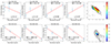 |
Fig. A.1. Linear fit of 4 pixels in the RM maps, from left to right. |
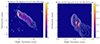 |
Fig. A.2. Goodness of fit using reduced chi squared values of both RM maps. |
Appendix B: Observational information summary
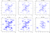 |
Fig. B.1. Fourier coverages of all frequencies. |
All Figures
|
Fig. 1. VLBA total and linear polarisation images at different frequencies. Contours show total intensity above a threshold of 5σ; colour scale represents the linearly polarised intensity above 4σ; white ticks indicate the observed electric vector position angle. The peak value of total flux density is 2.83, 2.67, 1.55, 2.08, 3.89, 2.42 Jy/beam for 5, 8, 15, 22, 43, and 86 GHz, respectively. The corresponding rms is 12.55, 4.01, 1.96, 1.23, 2.64, and 5.49 mJy/beam. |
| In the text | |
|
Fig. 2. Rotation measure maps of 3C 273 using 5–8–15 GHz (left column, top) and 15–22–43 GHz (left column, bottom) and its respective errors (right column). Corrected (intrinsic) EVPAs are plotted as dark blue ticks. |
| In the text | |
|
Fig. 3. Transversal sections for total intensity image at 5 GHz (top row), linear polarisation at 5 GHz (central row), and degree of polarisation (bottom row). Units are displayed in the left column. The order of the sections along the jet is numbered in the total intensity image. |
| In the text | |
|
Fig. 4. Transversal sections for RM map using 5–8–15 GHz (top row) and 15–22–43 GHz (bottom row). The order and values of the sections are displayed from left to right, as shown in Figure 3. |
| In the text | |
|
Fig. A.1. Linear fit of 4 pixels in the RM maps, from left to right. |
| In the text | |
|
Fig. A.2. Goodness of fit using reduced chi squared values of both RM maps. |
| In the text | |
|
Fig. B.1. Fourier coverages of all frequencies. |
| In the text | |
Current usage metrics show cumulative count of Article Views (full-text article views including HTML views, PDF and ePub downloads, according to the available data) and Abstracts Views on Vision4Press platform.
Data correspond to usage on the plateform after 2015. The current usage metrics is available 48-96 hours after online publication and is updated daily on week days.
Initial download of the metrics may take a while.