| Issue |
A&A
Volume 692, December 2024
|
|
|---|---|---|
| Article Number | A148 | |
| Number of page(s) | 11 | |
| Section | Interstellar and circumstellar matter | |
| DOI | https://doi.org/10.1051/0004-6361/202451981 | |
| Published online | 10 December 2024 | |
Dust mass in protoplanetary disks with porous dust opacities
1
School of Physical Science and Technology, Southwest Jiaotong University,
Chengdu
610031,
China
2
Purple Mountain Observatory, Chinese Academy of Sciences,
10 Yuanhua Road,
Nanjing
210023,
China
3
Institut d’Astrophysique de Paris, Sorbonne Université, CNRS (UMR7095),
75014
Paris,
France
4
Max-Planck-Institut für Astronomie,
Königstuhl 17,
69117
Heidelberg,
Germany
5
Institut für Theoretische Physik und Astrophysik, Christian-Albrechts-Universität zu Kiel,
Leibnizstr. 15,
24118
Kiel,
Germany
6
Sterrenkundig Observatorium, Ghent University,
Krijgslaan 281-S9,
9000
Gent,
Belgium
7
Institute for Astronomy, School of Physics, Zhejiang University,
866 Yu Hang Tang Road, Hangzhou,
Zhejiang
310027,
China
★ Corresponding author; This email address is being protected from spambots. You need JavaScript enabled to view it.
Received:
25
August
2024
Accepted:
30
October
2024
Abstract
Atacama Large Millimeter/submillimeter Array surveys have suggested that protoplanetary disks are not massive enough to form the known exoplanet population, based on the assumption that the millimeter continuum emission is optically thin. In this work, we investigate how the mass determination is influenced when the porosity of dust grains is considered in radiative transfer models. The results show that disks with porous dust opacities yield similar dust temperatures, but systematically lower millimeter fluxes, as compared to disks that incorporate compact dust grains. Moreover, we have recalibrated the relation between dust temperature and stellar luminosity for a wide range of stellar parameters. We also calculated the dust masses of a large sample of disks using the traditionally analytic approach. The median dust mass from our calculation is about six times higher than the literature result, and this is mostly driven by the different opacities of porous and compact grains. A comparison of the cumulative distribution function between disk dust masses and exoplanet masses shows that the median exoplanet mass is about two times lower than the median dust mass when grains are assumed to be porous and there are no exoplanetary systems with masses higher than the most massive disks. Our analysis suggests that adopting porous dust opacities may alleviate the mass budget problem for planet formation. As an example illustrating the combined effects of optical depth and porous dust opacities on the mass estimation, we conducted new IRAM/NIKA-2 observations toward the IRAS 04370+2559 disk and performed a detailed radiative transfer modeling of the spectral energy distribution (SED). The best-fit dust mass is roughly 100 times higher than the value given by a traditionally analytic calculation. Future spatially resolved observations at various wavelengths are required to better constrain the dust mass.
Key words: radiative transfer / protoplanetary disks / circumstellar matter
© The Authors 2024
 Open Access article, published by EDP Sciences, under the terms of the Creative Commons Attribution License (https://creativecommons.org/licenses/by/4.0), which permits unrestricted use, distribution, and reproduction in any medium, provided the original work is properly cited.
This article is published in open access under the Subscribe to Open model. This email address is being protected from spambots. You need JavaScript enabled to view it. to support open access publication.
1 Introduction
Despite the fact that dust grains occupy only about 1% of the total disk mass, they stand as crucial ingredients that influence multiple aspects of disk evolution and planet formation (e.g., Natta et al. 2007; Birnstiel 2023). First, dust opacity dominate over gas opacity; therefore, dust grains play an important role in setting the thermal and geometrical structure of disks. Second, dust particles provide the surface area upon which complex chemical reactions take place (e.g., Garrod & Herbst 2006; Henning & Semenov 2013; Öberg et al. 2023). Dust particles also act as carriers to redistribute volatile species within the disk via dust diffusion, settling, and radial drift (e.g., Krijt et al. 2016; Stammler et al. 2017; Eistrup & Henning 2022). Finally, dust grains are the building blocks for the formation of planetesimals, terrestrial planets, and the cores of giant planets. Consequently, the total amount of dust content is among the key properties that characterize the potential for planet formation.
Estimating dust mass is commonly accomplished by millimeter continuum observations. Thanks to the high sensitivity of the Atacama Large Millimeter/submillimeter Array (ALMA), a large sample of about 1000 disks located in nearby star-forming regions have been observed at millimeter wavelengths, (e.g., Ansdell et al. 2016; Barenfeld et al. 2016; Pascucci et al. 2016; Cazzoletti et al. 2019; Tazzari et al. 2021; Grant et al. 2021). Assuming the emitting dust is optically thin and isothermal, the measured flux density, Fν, can be converted into dust masses via the analytic formula:
![Mathematical equation: $\[M_{\text {dust }}=\frac{F_{\nu} D^{2}}{\kappa_{\nu} B_{\nu}\left(T_{\text {dust }}\right)},\]$](/articles/aa/full_html/2024/12/aa51981-24/aa51981-24-eq1.png) (1)
(1)
where Bν(Tdust) stands for the Planck function given at the observed frequency ν and dust temperature Tdust, D refers to the distance to the object, and κν is the mass absorption coefficient. Based on Eq. (1), Andrews (2020) built the cumulative distribution function (CDF) of Mdust for 887 disks, finding that less than ~10% disks have enough material to produce our solar system or its analogs in the exoplanet population. Similarly, Manara et al. (2018) find that exoplanetary system masses are comparable or even higher than the most massive disks with ages of ~1–3 Myr. Although the discrepancy between the disk and exoplanets mass distributions is mitigated by accounting for observational selection and detection biases (Mulders et al. 2021), the findings by Andrews (2020) and Manara et al. (2018) naturally raise a conundrum that protoplanetary disks do not have enough mass to make planetary systems. This puzzle is referred as the “mass budget problem” of planet formation in the literature.
Several proposed solutions have been considered across three plausible scenarios. The first suggests that planet formation might begin at earlier stages of disk evolution than previously thought. The prevalence of substructures in protostellar disks is the supporting evidence (Segura-Cox et al. 2020; Sheehan et al. 2020; Ohashi et al. 2023; Hsieh et al. 2024), since disk substructures can be created by planets (Kley & Nelson 2012; Paardekooper et al. 2023). Moreover, young disks in the Class 0/I phases are generally more massive than Class II disks (Tychoniec et al. 2018, 2020), providing more material for planet formation. The second scenario assumes that the disk acts as a conveyor belt that transports material from the environment to the central star (Manara et al. 2018; Gupta et al. 2023, 2024). Thus, the total amount of material available for planet formation actually exceeds the observed value. The third proposal argues that Mdust estimated using Eq. (1) is merely a lower limit (e.g., Ballering & Eisner 2019) because protoplanetary disks are not necessarily optically thin at millimeter wavelengths (e.g., Liu et al. 2017; Rilinger et al. 2023; Xin et al. 2023). Recently, Savvidou & Bitsch (2024) showed that the early formation of giant planets is expected to create pressure bumps exterior to the planetary orbit, which will trap the inward drifting dust. The trapped dust will be largely unaccounted for by the approximation of optically thin emission. Assuming dust grains are compact spheres, Liu et al. (2022) demonstrate that the disk outer radius, inclination, and true dust mass are most important to create optically thick regions, resulting in mass underestimations from a few to hundreds times.
Theoretical studies show that dust grains in protoplanetary disks might be porous in the process of coagulation and growth (e.g., Dominik & Tielens 1997; Wurm & Blum 1998) and grain growth via porous aggregates can overcome the radial drift barrier to form planetesimals (Okuzumi et al. 2012; Kataoka et al. 2013; Michoulier et al. 2024). The existence of porous dust grains is observationally supported. Near-infrared (NIR) scattered light observations show that the polarization phase functions are consistent with model predictions incorporating micron-sized porous dust grains (e.g., Stolker et al. 2016; Ginski et al. 2023; Tazaki et al. 2023). A detailed analysis of multiwavelength continuum and millimeter polarization observations of the HL Tau disk indicates that dust grains are porous, and the porosity ranges from 70% to 97% depending on the best-fit grain size (Zhang et al. 2023).
The absorption and scattering coefficients of porous dust grains are different from those of compact spherical particles (e.g., Kirchschlager & Wolf 2014; Ysard et al. 2018; Kirchschlager et al. 2019), which have a direct impact on the radiative transfer process in protoplanetary disks. In this work, using self-consistent radiative transfer models, we investigate how porous dust opacities influence the dust temperature, emergent millimeter flux, and therefore the estimation of Mdust. The setup of the radiative transfer models and the resulting trends are presented in Sect. 2. In Sect. 3, we apply porous dust opacities to the calculation of Mdust for a large number of disks and we compare the CDF between the disk sample and the exoplanet population investigated by Mulders et al. (2021). As an application, we model the spectral energy distribution (SED) of the IRAS 04370+2559 disk in Sect. 4. The paper concludes with a summary in Sect. 5.
2 Radiative transfer models
In this section, we first give an introduction about the setup of the radiative transfer model and we then built a grid of models by sampling a few key parameters that have prominent effects on the dust temperature and millimeter flux.
2.1 Dust density structure
We considered a flared disk that includes two distinct dust grain populations, namely, a small grain population (SGP) and a large grain population (LGP). We fixed the disk inner radius Rin to 0.1 AU, which is close to the dust sublimation radius of a typical T Tauri star. The SGP occupies a small fraction of the dust mass, (1 − f) Mdust, and its scale height follows a power law of
![Mathematical equation: $\[h=h_{100} \times\left(\frac{R}{100 ~\mathrm{AU}}\right)^{\Psi}.\]$](/articles/aa/full_html/2024/12/aa51981-24/aa51981-24-eq2.png) (2)
(2)
The flaring index is denoted with Ψ, while h100 refers to the scale height at a radial distance of R = 100 AU. On the contrary, the LGP has a mass of f Mdust and so, it dominates the dust mass and is concentrated close to the midplane with a scale height of Λ h. The degree of dust settling is characterized by setting Λ = 0.2 (Andrews et al. 2011). To distribute the mass for the SGP and LGP, we adopted f = 0.85, which is a typical value found from multiwavelength modeling of protoplanetary disks (e.g., Andrews et al. 2011; van der Marel et al. 2018; Schwarz et al. 2021; Zhang et al. 2021). The dust surface density is assumed to be a power law with an exponential taper
![Mathematical equation: $\[\Sigma(R)=\Sigma_{c}\left(\frac{R}{R_{c}}\right)^{-\gamma} \exp \left[-\left(\frac{R}{R_{c}}\right)^{2-\gamma}\right],\]$](/articles/aa/full_html/2024/12/aa51981-24/aa51981-24-eq3.png) (3)
(3)
where γ is the gradient parameter, and Rc is a characteristic radius. This is the similarity solution for disk evolution, which assume that the viscosity has a power-law radial dependence and is independent of time (Lynden-Bell & Pringle 1974). The proportionality factor, Σc, is determined by normalizing the total dust mass Mdust. We truncated the disk at an outer radius of 8 Rc. The dust volume density is parameterized as:
![Mathematical equation: $\[\rho_{\mathrm{SGP}}(R, z)=\frac{(1-f) \Sigma(R)}{\sqrt{2 \pi} h} ~\exp \left[-\frac{1}{2}\left(\frac{z}{h}\right)^{2}\right],\]$](/articles/aa/full_html/2024/12/aa51981-24/aa51981-24-eq4.png) (4)
(4)
![Mathematical equation: $\[\rho_{\mathrm{LGP}}(R, z)=\frac{f \Sigma(R)}{\sqrt{2 \pi} \Lambda h} \exp \left[-\frac{1}{2}\left(\frac{z}{\Lambda h}\right)^{2}\right].\]$](/articles/aa/full_html/2024/12/aa51981-24/aa51981-24-eq5.png) (5)
(5)
Table 1 summarizes the parameters of the model.
2.2 Dust properties
The dust ensemble is composed of water ice (Warren & Brandt 2008), astronomical silicates (Draine 2003), troilite (Henning & Stognienko 1996), and refractory organic material (Henning & Stognienko 1996), with volume fractions being 36%, 17%, 3%, and 44%, respectively. The optical constants of each individual are mixed using the Bruggeman mixing rule (Bruggeman 1935). The resulting optical constants are referred as the DSHARP dust model (Birnstiel et al. 2018). The bulk density of the mix is ρs.compact = 1.675 g/cm3. To have porous grains, we adopted the effective medium theory (EMT) and mixed the DSHARP dust composition with vacuum using the Bruggeman mixing rule. The mixed complex refractive indices are used to calculate dust absorption and scattering properties with the Mie theory and OpTool (Dominik et al. 2021). The porosity, 𝒫, controls the volume fraction of vacuum. We chose 𝒫 = 0.8, a value consistent with current observations of protoplanetary disks (e.g., Zhang et al. 2023) and the cometary nucleus 67P/Churyumov–Gerasimenko (Kofman et al. 2015; Jorda et al. 2016). The bulk density of the porous dust grains is ρs.porous = (1 − 𝒫) ρs.compact = 0.335 g/cm3. We note that compact dust particles can be considered as a limiting case of 𝒫 = 0.
We defined an effective radius that is the radius of a volume-equivalent solid sphere, aeff = a (1 − 𝒫)1/3, where a is the grain size. In this work, we compare compact dust opacities with porous dust opacities, while assuming that both types of dust grains have the same effective radius, aeff. In the literature, the characteristic radius, ac = a (1 − 𝒫), has been proposed as another choice for describing the size-dependent dust opacities (Tazaki et al. 2019a; Zhang et al. 2023). For 𝒫 = 0.8, aeff and ac differ by a factor of ~3. The effective grain size distribution follows the power law ![Mathematical equation: $\[\mathrm{d} n(a_{\text {eff }}) \propto a_{\text {eff }}^{-3.5} \mathrm{~d} a_{\text {eff }}\]$](/articles/aa/full_html/2024/12/aa51981-24/aa51981-24-eq9.png) with a minimum effective grain size fixed to
with a minimum effective grain size fixed to ![Mathematical equation: $\[a_{\min }^{\text {eff }}\]$](/articles/aa/full_html/2024/12/aa51981-24/aa51981-24-eq10.png) = 0.01 μm. For the SGP, the maximum effective grain size is set to
= 0.01 μm. For the SGP, the maximum effective grain size is set to ![Mathematical equation: $\[a_{\max }^{\text {eff }}\]$](/articles/aa/full_html/2024/12/aa51981-24/aa51981-24-eq11.png) = 1 μm. For the LGP, we adopt
= 1 μm. For the LGP, we adopt ![Mathematical equation: $\[a_{\max }^{\text {eff }}\]$](/articles/aa/full_html/2024/12/aa51981-24/aa51981-24-eq12.png) = 1 mm accounting for grain growth commonly identified in protoplanetary disks. The porosity may not be uniform due to the dust coagulation of the SGP into the LGP. However, we focus only on the simplest scenario where the SGP and LGP are assumed to have the same porosity of 𝒫 = 0.8.
= 1 mm accounting for grain growth commonly identified in protoplanetary disks. The porosity may not be uniform due to the dust coagulation of the SGP into the LGP. However, we focus only on the simplest scenario where the SGP and LGP are assumed to have the same porosity of 𝒫 = 0.8.
Panel a of Fig. 1 shows the mass absorption coefficient at 1.3 mm (κ1.3 mm) as a function of ![Mathematical equation: $\[a_{\max }^{\text {eff }}\]$](/articles/aa/full_html/2024/12/aa51981-24/aa51981-24-eq13.png) . As can be seen, κ1.3mm of porous grains is lower than that of compact grains1. For
. As can be seen, κ1.3mm of porous grains is lower than that of compact grains1. For ![Mathematical equation: $\[a_{\max }^{\text {eff }}\]$](/articles/aa/full_html/2024/12/aa51981-24/aa51981-24-eq14.png) = 1 mm, porous grains feature κ1.3mm = 0.37 cm2/g that is five times lower than compact grains with κ1.3mm = 1.86 cm2/g, which will have a direct impact on the mass estimation, see Eq. (1). The differences in κν between porous grains and compact grains are less pronounced in the optical regime, see panel c of Fig. 1. This implies that Tdust obtained from the radiative transfer simulation will not differ too much between the two types of grains because most of the stellar energy emits at optical wavelengths. The opacity slope, for instance, β1.3–3 mm measured between 1.3 mm and 3 mm, behaves differently between compact grains and porous grains. For compact grains, there is a peak around
= 1 mm, porous grains feature κ1.3mm = 0.37 cm2/g that is five times lower than compact grains with κ1.3mm = 1.86 cm2/g, which will have a direct impact on the mass estimation, see Eq. (1). The differences in κν between porous grains and compact grains are less pronounced in the optical regime, see panel c of Fig. 1. This implies that Tdust obtained from the radiative transfer simulation will not differ too much between the two types of grains because most of the stellar energy emits at optical wavelengths. The opacity slope, for instance, β1.3–3 mm measured between 1.3 mm and 3 mm, behaves differently between compact grains and porous grains. For compact grains, there is a peak around ![Mathematical equation: $\[a_{\max }^{\text {eff }}\]$](/articles/aa/full_html/2024/12/aa51981-24/aa51981-24-eq15.png) ~ λ/2π due to the unique feature of Mie interference. For larger grain sizes, the opacity slope monotonically decreases with
~ λ/2π due to the unique feature of Mie interference. For larger grain sizes, the opacity slope monotonically decreases with ![Mathematical equation: $\[a_{\max }^{\text {eff }}\]$](/articles/aa/full_html/2024/12/aa51981-24/aa51981-24-eq16.png) . If the dust emission is optically thin and in the Rayleigh-Jeans tail, the opacity slope is linked to millimeter spectral indices (α) via β = α − 2. This is the reason why dust grain sizes can be probed by multiwavelength millimeter observations (e.g., Ricci et al. 2010; Williams & Cieza 2011). However, if the dust particles are porous, the grain size becomes difficult to be constrained because the opacity slope is less sensitive to
. If the dust emission is optically thin and in the Rayleigh-Jeans tail, the opacity slope is linked to millimeter spectral indices (α) via β = α − 2. This is the reason why dust grain sizes can be probed by multiwavelength millimeter observations (e.g., Ricci et al. 2010; Williams & Cieza 2011). However, if the dust particles are porous, the grain size becomes difficult to be constrained because the opacity slope is less sensitive to ![Mathematical equation: $\[a_{\max }^{\text {eff }}\]$](/articles/aa/full_html/2024/12/aa51981-24/aa51981-24-eq17.png) , as described in panel b of our Fig. 1 or Fig. 3 of Miotello et al. (2023).
, as described in panel b of our Fig. 1 or Fig. 3 of Miotello et al. (2023).
As described above, we modeled the porosity as a certain percentage of vacuum inclusion in dust grains by using the EMT, and calculated the dust properties with the Mie theory. A more sophisticated approach is to define the porosity by a size of void inclusion and a volume-filling factor (e.g., Kirchschlager & Wolf 2014; Kirchschlager et al. 2019). In this way, dust properties of porous grains can be calculated with the DDSCAT code (Draine & Flatau 1994, 2010) by applying the discrete dipole approximation (Purcell & Pennypacker 1973). Kirchschlager & Wolf (2013) showed that absorption cross-sections of micron-sized grains calculated with the Mie theory and DDSCAT code differ for λ < 0.2 μm and λ > 20 μm. Comparisons for millimeter-sized grains are difficult, because running the DDSCAT code for grains with large size parameters (2πa/λ) is time-consuming, and the reliability of results needs to be validated as well. Hence, we left it as a future direction to investigate the difference in the dust temperature between the two approaches and how it would impact the estimation of dust mass.
Fixed and varied parameters of the model grid.
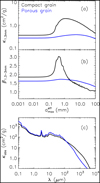 |
Fig. 1 Dust properties considered in this work. Panel a: mass absorption coefficient at λ = 1.3 mm as a function of |
![Mathematical equation: $\[a_{\max }^{\text {eff }}\]$](/articles/aa/full_html/2024/12/aa51981-24/aa51981-24-eq18.png)
![Mathematical equation: $\[\mathrm{d} n(a_{\text {eff }}) \propto a_{\text {eff }}^{-3.5} \mathrm{~d} a_{\text {eff }}\]$](/articles/aa/full_html/2024/12/aa51981-24/aa51981-24-eq19.png)
![Mathematical equation: $\[a_{\min }^{\text {eff }}\]$](/articles/aa/full_html/2024/12/aa51981-24/aa51981-24-eq20.png)
![Mathematical equation: $\[a_{\max }^{\text {eff }}\]$](/articles/aa/full_html/2024/12/aa51981-24/aa51981-24-eq21.png)
2.3 Heating mechanisms
Stellar irradiation and viscous accretion are major heating sources for protoplanetary disks. Viscous heating mainly affects the temperature distribution in the interior portion of the inner disk, for instance, R ≲ 2 AU (Hartmann 2009; Harsono et al. 2015). However, the main disk mass reservoir is in the cold outer disk. Therefore, we only considered stellar irradiation in the simulation.
In Sect. 4, we describe our detailed fitting to the SED of IRAS 04370+2559, which is a T Tauri star located in the Taurus star formation region. For convenience, we adopted its stellar luminosity and effective temperature (L⋆ = 0.86 L⊙, Teff = 3778 K, see Sect. 4.1) in creating the model grid. We take the distance of D = 140 pc to scale the simulated observable. We note that using different stellar properties will not have a significant impact on the trends of Tdust and millimeter Fν with parameters explored in this work. The stellar spectrum is taken from the BT-Settl database (Allard et al. 2011), assuming a surface gravity of log g = 3.5 and solar metallicity.
2.4 Establishment of the model grid
To build a grid of models, we explored a few key parameters that are expected to have the most significant impact on Tdust and the millimeter flux, Fν. The flaring index, Ψ, and scale height, h100, work together to determine the disk geometry, thereby altering the total amount of stellar energy absorbed by the disk; this, in turn, goes on to affect Tdust and Fν. As shown by Liu et al. (2022), the true Mdust, disk size, and disk inclination (i) are most important parameters for creating optically thick regions. Accordingly, Mdust and Rc have an impact on the mass estimation. The disk inclination affects the optical depth along the line of sight, therefore altering the millimeter Fν. We refer to Liu et al. (2022) for details about the role of this parameter in determining the dust mass. For simplicity, we fixed i = 30° throughout this work.
We sampled the above-mentioned four parameters (Ψ, h100, Mdust and Rc) within reasonable ranges that are consistent with results derived from multiwavelength observations and modeling of protoplanetary disks (e.g., Andrews et al. 2011; Kirchschlager et al. 2016; Andrews et al. 2013; Liu et al. 2019). For parameters with a broad dynamical range, the sampling is performed in a logarithmic manner, whereas parameters with a narrow dynamical range are sampled in the linear space. The grid points in each dimension are tabulated in Table 1. There are 9360 models in total. We ran the simulations separately using the compact dust opacities and porous dust opacities.
The well-tested RADMC-3D2 package is invoked to solve the problem of continuum radiative transfer (Dullemond et al. 2012). Dust scattering is taken into account since literature works have demonstrated that it is able to reduce the emission from optically thick regions (Zhu et al. 2019; Sierra & Lizano 2020) and influence the millimeter spectral index (Liu 2019). We first ran the thermal Monte-Carlo simulation, from which the mass-averaged dust temperature, Tdust, was obtained. Then, we simulated the flux densities from optical to millimeter wavelengths and the 0.88 mm images. The 0.88 mm images are used to derive an effective disk radius that is the radius at which a given fraction of the cumulative flux is contained. Following Tripathi et al. (2017), we computed the radius encircling 68% of the total flux. Finally, we compared our results with those measured on observed millimeter images of Taurus disks (Hendler et al. 2020).
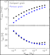 |
Fig. 2 Comparison of F1.3mm (upper panel) and Tdust (bottom panel) between models that use compact dust opacities (black) and porous dust opacities (blue), respectively. In the models, all of other parameters are fixed: Rc = 30 AU, Ψ = 1.15, H100 = 10 AU. |
2.5 Results
Figure 2 shows the mass-averaged dust temperature (Tdust) and flux density at 1.3 mm (F1.3mm) as a function of Mdust. The difference in Tdust between compact dust opacities and porous dust opacities is less than ~1 K. In self-consistent radiative transfer modeling, only upper disk layers are directly illuminated by the central star, resulting in hot and warm upper disk layers. Generally, such hot-warm disk regions lie above the disk photosphere, where the radial optical depth at 0.55 μm is equal to unity (i.e., τradial.0.55 μm = 1), which is indicated with the grey lines in Fig. 3. The interior disk regions are indirectly heated by both the radiation that is scattered from above towards the midplane and the reemission of the hot and warm layers. The former heating mechanism is mainly relevant to the optical cross-section, while the IR cross-section is important for the latter heating process. As shown in panel c of Fig. 1, porous dust grains feature higher optical cross-sections, leading to a lower Tdust. However, porous dust grains also have larger IR cross-sections. Hot and warm layers will re-emit more IR emission and therefore compensate for the reduced Tdust. These facts explain the small difference in Tdust between both types of dust grains. Models with porous dust opacities produce systematically lower F1.3mm than those with compact dust opacities. This is driven by the difference in the dust opacity, see panel a of Fig. 1. For each of the 9360 models in the grid, we can calculate the ratio of F1.3mm with porous grains to that with compact grains. We derived a median value of 0.4. We observed a less than linear scaling relation between F1.3mm and Mdust. This outcome can be explained in two plausible ways. First, the higher optical depth with larger Mdust value results in a stronger shielding of the inner disk regions and a lower mass-averaged dust temperature as a result. For more details, we refer to the comparison of the τradial.0.55 μm = 1 surface between two models with different Mdust in Fig. 3. Second, with the increasing Mdust, the millimeter optical depth increases as well, which will hide more disk interior regions and thus their reemitted flux (see the vertical optical depth at a wavelength of 1.3 mm in Fig. 3). When the disk becomes optically thick, the millimeter emission gradually saturates. Therefore, the difference in F1.3mm decreases as we approach a higher Mdust.
The disk’s inner radius is fixed in the model grid. In this case, the disk outer radius defines the radial range in which dust grains are confined and it significantly affects the optical depth and, consequently, the mass estimation. From the observational point of view, the disk outer radius is commonly characterized by the effective disk radius from spatially resolved images. Previous studies have found a strong correlation between the effective disk radius and millimeter flux density (e.g., Tripathi et al. 2017; Andrews et al. 2018; Hendler et al. 2020). Using the 0.88 mm images, we computed the effective disk radius R68 (i.e., the radius enclosing 68% of the total flux) to connect the statistics of our models to those obtained from observations in the literature. The results are presented in Fig. 4. The effective disk radius depends mainly on the radial optical depth that is determined by the dust opacity and surface density (see Eq. (3)). As can be seen in the upper panel, R68 increases with the characteristic radius, Rc. Moreover, the range of R68 for each sampled Rc, indicated by the vertical length of the bars, is similar for models with the two types of grains. In the bottom panel of the figure, the blue curve and grey curve depict the boundaries within which the 7920 models with porous dust opacities and compact dust opacities occupy in the R68 − F0.88mm diagram, respectively. Broadly, the blue curve is a shift of the grey curve towards the lower flux direction. Hendler et al. (2020) found that R68 correlates with F0.88mm via log R68 = 2.16 + 0.53 log F0.88mm for Taurus disks. Such a correlation, shown with the dashed line, is consistent with the trend revealed by our models.
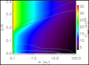 |
Fig. 3 Dust temperature of a representative model with parameters of Mdust = 10−4 M⊙, Rc = 30 AU, Ψ = 1.15, and H100 = 10 AU. For a better representation, we show the quantity |
![Mathematical equation: $\[\sqrt{T_{\text {dust }}}\]$](/articles/aa/full_html/2024/12/aa51981-24/aa51981-24-eq22.png)
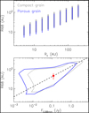 |
Fig. 4 Statistics of the effective disk radius R68 from the model grid. Upper panel: ranges of R68 for each of the sampled Rc. The blue lines refer to the result when porous dust grains are considered, whereas the grey lines represent the case by using compact dust opacities. The thickness of lines is only for a better illustration. Bottom panel: relation between R68 and F0.88mm. The blue curve and grey curves enclose the regions occupied by the 9360 models with porous grains and compact grains, respectively. The dashed line shows the relation log R68 = 2.16 + 0.53 log F0.88mm (Hendler et al. 2020). The red dot indicates the expected position of IRAS 04370+2559 in the diagram; for details, see Sect. 4.2. |
3 Solid mass budget for planet formation
Based on self-consistent radiative transfer modeling, we have demonstrated that models with porous dust grains are systematically fainter in the millimeter domain, but the dust temperature is similar to the case of compact grains. These facts have an impact on the solid mass budget for planet formation. In this section, we calculate Mdust for a large sample of disks using Eq. (1) and we compare the CDF of Mdust with that of exoplanet masses.
Manara et al. (2023) collected 0.88 mm and/or 1.3 mm flux densities for a large number of nearby disks. Assuming κν = 2.3(ν/230 GHz) cm2/g and a constant Tdust = 20 K, they investigated the statistics of Mdust calculated with Eq. (1). In this work, we focus on the 718 disks with a similar age (i.e., 1–3 Myr) in their sample, which are located in the Taurus, Lupus, Chamaeleon, and Ophiuchus molecular clouds. The stellar luminosity of these sources spans a broad range, from 10−3 L⊙ ≲ L⋆ ≲ 100 L⊙; therefore, taking a constant Tdust value is not appropriate. Andrews et al. (2013) showed that Tdust mainly depends on L⋆, and derived a relation Tdust = 25 (L⋆/L⊙)0.25 K. Nevertheless, their results are based on radiative transfer models with a limited range of 0.1 L⊙ ≲ L⋆ ≲ 100 L⊙. The scaling of Tdust with L⋆ in the lower stellar mass regime was further investigated by van der Plas et al. (2016) and Hendler et al. (2017). The relation is found to be flatter Tdust = 22 (L⋆/L⊙)0.16 K (van der Plas et al. 2016).
To homogenize our analysis, we re-calibrated the Tdust − L⋆ relation from massive young stars all the way down to the brown dwarf regime by creating a grid of radiative transfer models. The modeling framework is identical to that described in Sect. 2 and porous dust opacities were used in the simulation. We first sampled 34 values of L⋆ that are logarithmically distributed in the range of [10−3 L⊙, 100 L⊙]. Then, we interpolated the 2.5 Myr isochrone of pre-main-sequence evolutionary tracks to obtain Teff and M⋆. For L⋆ < 0.4 L⊙ (at approximately Teff < 3900 K), we adopted the models presented by Baraffe et al. (2015); whereas we took the nonmagnetic evolutionary models by Feiden (2016) for L⋆ ≥ 0.4 L⊙. This procedure is motivated by the fact that the two sets of isochrones overlap well around Teff ~ 3900 K. Once the stellar parameters are given, we can use the corresponding BT-Settl models to represent the atmospheric spectra (Allard et al. 2011). In the grid, there are three points for Ψ: 1.05, 1.15, and 1.25. We considered three values for h100: 5 AU, 10 AU, and 15 AU. For Rc, we also sampled three values: 10 AU, 30 AU, and 100 AU. We considered three disk-to-stellar mass ratios, namely, 0.001, 0.01, and 0.1. Then, Mdust for each model is determined by assuming a gas-to-dust mass ratio of 100.
Figure 5 shows the mass-averaged dust temperature Tdust as a function of L⋆. Although there is a large dispersion in Tdust for each L⋆ bin, an obvious trend is observed, with cooler disks around fainter stars. Moreover, the decreasing tendency of Tdust with L⋆ appears steeper for stars with L⋆ ≳ 0.2 L⊙ than that for systems with lower luminosities. The same phenomenon is also seen in Fig. 17 of Andrews et al. (2013), in which the dust temperature decrease seems to flatten out toward the low luminosity regime. We fit a polynomial (at second order) to the correlation between Tdust and L⋆. The best fit is represented by
![Mathematical equation: $\[\log T_{\text {dust }}=1.445+0.224 ~\log~ L_{\star}+0.013\left(\log L_{\star}\right)^{2}.\]$](/articles/aa/full_html/2024/12/aa51981-24/aa51981-24-eq23.png) (6)
(6)
Our relation for L⋆l < 0.2 L⊙ predicts a similar dust temperature to the result given by van der Plas et al. (2016), whereas for L⋆ ≳ 0.2 L⊙, we obtained similar dust temperature to the prescription of Andrews et al. (2013). The small difference between our and literature results is understood because of the difference in the choice of dust density distribution, disk parameters, and dust opacities. For instance, we used porous dust opacities in the modeling, while other studies adopted compact dust opacities. Moreover, whether or not taking into account the stellar-mass dependent disk outer radius (Andrews et al. 2018; Andrews 2020) and interstellar radiation will also influence the heating of disks as a function of spectral type and, therefore, affect the Tdust − L⋆ relation (e.g., van der Plas et al. 2016; Hendler et al. 2017).
To calculate Mdust, we directly took L⋆, Fν and D of each target provided by Manara et al. (2023). When L⋆ is not available, we set Tdust = 20 K. The measured flux density at 1.3 mm is used with a higher priority since the optical depth is lower at longer wavelengths. The mass absorption coefficients of porous grains for the LGP were adopted in the calculation, namely: κ1.3mm = 0.37 cm2/g and κ0.88mm = 0.84 cm2/g. As can be seen in the upper panel of Fig. 6, adopting porous dust opacities results in a systematically higher Mdust values than those calculated by assuming κν = 2.3 (ν/230 GHz) cm2/g and a constant Tdust = 20 K. Moreover, we used the Kaplan–Meier estimator from the ASURV package to estimate the CDFs and median dust masses while properly accounting for the upper limits (Feigelson & Nelson 1985; Isobe et al. 1986). The median values are 1.6 M⊕ and 9.3 M⊕ for Mdust calculated by Manara et al. (2023) and in this study, respectively, which means that dust masses in protoplanetary disks may be underestimated by a factor of ~6 if the grains are in fact porous and not compact. For comparison, the grey curve in the bottom panel of Fig. 6 shows the CDF of Mdust calculated with the porous dust opacities and a constant dust temperature Tdust = 20 K. The distribution is similar to that derived by scaling Tdust with L⋆. This is understood because the disks have a wide range of stellar luminosity, 10−3 L⊙ ≲ L⋆ ≲ 100 L⊙, and the effect of dust temperature on the distribution smooths out when the analysis is performed in a large sample scale. Mulders et al. (2021) analyzed the mass distribution of the exoplanet population detected from the Kepler transit survey (e.g., Borucki et al. 2010; Thompson et al. 2018) and radial velocity surveys from Mayor et al. (2011) since both surveys have a well-characterized detection bias. The red curve in the bottom panel of Fig. 6 refers to the CDF of the exoplanet mass when accounting for observational selection and detection biases. The median mass of the exoplanets is 4.2 M⊕, which is about two times lower than the median dust mass calculated in this work. Moreover, we do not see any exoplanetary systems with masses higher than the most massive disks. Our study shows that if dust grains in disks are porous, the problem of insufficient mass for planet formation raised in the ALMA era may be resolved.
In the above analysis, we adopted an effective maximum grain size of 1 mm. The grain size has a direct impact on the dust opacity, and is commonly investigated via the millimeter spectral index (e.g., Andrews & Williams 2005; Ricci et al. 2010). Future observations at multiple (sub)millimeter wave-lengths are needed to constrain the grain size that is essential for a better characterization of the dust mass distribution. To observationally prove that dust grains are porous and constrain the porosity, 𝒫, multiwavelength observations and analyses are mandatory.
Grain porosity alters the absorption, scattering and polarization behavior of dust grains (e.g., Semenov et al. 2003; Ysard et al. 2018) and, therefore, influences the observable appearance of protoplanetary disks. The position, strengths, width, and shape of dust emission features in the mid-infrared (MIR) domain depend on the grain structure (e.g., Voshchinnikov & Henning 2008; Vaidya & Gupta 2011). The detailed decomposition of spectra obtained with the Infrared Spectrograph (IRS) on board Spitzer has demonstrated that the emission bands of forsterite and enstatite are best matched with porous grains, rather than compact spherical grains (e.g., Bouwman et al. 2008; Juhász et al. 2010). Analyzing the spectra from the Mid-Infrared Instrument (MIRI) equipped on JWST offers the same conclusion (e.g., Jang et al. 2024). The accumulating MIRI spectra will shed more insights into the dust properties particularly in faint disks that were not accessible by Spitzer.
Kirchschlager & Wolf (2014) found that grain porosity strongly influences the scattered-light maps of protoplanetary disks. For highly tilted disks (e.g., i ≳ 75°), the flux of the scattered light at optical wavelengths is significantly enlarged when porous dust opacities are included. Once the disk deviates from a face-on orientation (e.g., i ≳ 5°), the scattered light maps show a dark lane that is characteristic for inclined disks. The dark lane appears more pronounced assuming compact dust opacities. By analyzing scattered-light maps from radiative transfer simulations, Tazaki et al. (2019b) found that porous dust aggregates large compared to NIR wavelengths show marginally grey or slightly blue in total or polarized intensity, while large compact dust grains give rise to reddish scattered-light colours in total intensity. High-resolution NIR observations can be used to verify the model predictions (e.g., Fukagawa et al. 2010; Avenhaus et al. 2018).
Significant differences exist between polarimetric images of disks composed of porous particles and compact spheres (Min et al. 2012). Simulated polarization maps at optical wavelengths reveal an increase in the polarization degree by a factor of about four when porous grains are considered (Kirchschlager & Wolf 2014). The wavelength dependent polarization reversal (i.e., 90° flip of the polarization direction at visible light) depends strongly on the grain porosity; thus, it has diagnostic potential for dust properties. Tazaki et al. (2019a) investigated how the grain structure and porosity alter polarimetric images at millimeter wavelengths. The polarization pattern of disks containing moderately porous particles show near- and far-side asymmetries at (sub-)millimeter wavelengths. Porous grains exhibit a weaker wavelength dependence of scattering polarization than solid spherical grains. Brunngräber & Wolf (2021) investigated the effect of grain porosity on the polarization degree due to self-scattering in the (sub-)millimeter wavelength range. They found that porous dust grains with moderate filling factors of about 10% increase the degree of polarization by up to a factor of four compared to compact grains. However, the degree of polarization drops rapidly when the porosity is very high, with a filling factor of 1% or lower, because of the low opacity and optical depth. These theoretical studies show that multi-wavelength polarimetric observations are crucial to constrain the structure and porosity of dust grains in protoplanetary disks (e.g., Zhang et al. 2023; Ueda et al. 2024).
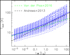 |
Fig. 5 Mass-averaged dust temperature as a function of stellar luminosity. The blue solid curve, expressed as log Tdust = 1.445 + 0.224 log L⋆ + 0.013 (log L⋆)2 is the best-fit relation to our models. The black dashed line refers to the relation Tdust = 25 (L⋆/L⊙)0.25 K presented by Andrews et al. (2013). The green dashed line shows the relation Tdust = 22 (L⋆/L⊙)0.16 K suggested by van der Plas et al. (2016). |
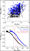 |
Fig. 6 Dust masses in protoplanetary disks and their statistics. Upper panel: Mdust as a function of M⋆. Black symbols show the results derived by Manara et al. (2023), while blue symbols represent our calculations considering porous dust opacities and a Tdust − L⋆ scaling given by Eq. (6), see Sect. 3. Millimeter detections are indicated with dots, whereas triangles mean upper limits of the millimeter flux are reported. The dashed line depicts the value of 100·Mdust = 0.01·M⋆. Bottom panel: CDF of Mdust. The grey curve shows the result calculated with porous dust opacities and a constant dust temperature Tdust = 20 K. The red curve refers to the distribution of exoplanet masses obtained by Mulders et al. (2021). The vertical dashed lines mark the median values of each distribution. |
4 Modeling the SED of IRAS 04370+2559
Protoplanetary disks, especially in the inner region and dense midplane, are likely to be optically thick at millimeter wavelengths (e.g., Wolf et al. 2008; Pinte et al. 2016; Liu et al. 2019; Ueda et al. 2020), which means that Mdust values calculated using Eq. (1) are underestimated. Therefore, in reality, the CDF of Mdust should shift towards the higher abscissa value in Fig. 6. Self-consistent radiative transfer modeling is an appropriate way to treat the optical depth effect and, therefore, to better constrain the dust mass. In this section, we describe how we conducted a detailed modeling of the SED of the IRAS 04370+2559 disk. We also showcase the difference in Mdust derived using different approaches and dust opacities.
4.1 Build the observed SED with new IRAM/NIKA-2 observations
IRAS 04370+2559 is a T Tauri star located in the Taurus star formation region at a distance of D = 137.4 pc (Gaia Collaboration 2023). Besides the fact that the stellar properties of IRAS 04370+2559 is representative for T Tauri stars (Gullbring et al. 1998), there are two reasons we selected it for the test. First, a large number of photometric data points from optical to millimeter regimes are available either in the archive or from our new IRAM/NIKA-2 observations. Second, the observed SED of IRAS 04370+2559, shown with red dots in panel a of Fig. 7, displays a flux drop at λ ~ 70 μm. This is a strong indication of dust settling (Liu et al. 2012; Dullemond & Dominik 2004; D’Alessio et al. 2006), which implies that a huge amount of material is very likely concentrated close to the disk midplane, creating high optical depths. In this case, a detailed modeling of the SED is necessary to constrain the dust mass, and it is expected to have a large difference in Mdust derived with different approaches. To compile the SED, we collect photometry from the Sloan Digital Sky Survey (Adelman-McCarthy & et al. 2011), 2MASS catalog (Skrutskie et al. 2006), Spitzer/IRAC, and MIPS measurements (Luhman et al. 2010; Rebull et al. 2010) as well as Herschel/PACS data (Ribas et al. 2017). In the millimeter, there are data points at 1.3 mm and 3 mm obtained with the Submillimeter Array (Andrews et al. 2013) and Combined Array for Research in Millimeter-wave Astronomy (Babaian 2020), respectively.
We conducted new IRAM/NIKA-2 observations towards the IRAS 04370+2559 disk. Details about the observation, data reduction and flux extraction are described in Appendix A. The measured flux densities at 1.1 mm and 2 mm are 58.2 ± 2.4 mJy and 23.9 ± 0.6 mJy, respectively. These efforts allow us to build the SED with an excellent wavelength coverage (see panel a of Fig. 7). Andrews et al. (2013) fit the optical part of the SED and derived Teff = 3778 K and L⋆ = 0.9 L⊙, assuming a distance of 140 pc. We rescaled their stellar luminosity by adopting the Gaia distance of D = 137.4 pc (Gaia Collaboration 2023), yielding L⋆ = 0.86 L⊙. Moreover, an extinction of AV = 10.65 mag is required to reproduce the optical photometry. We used the extinction law of Cardelli et al. (1989) with RV = 3.1.
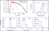 |
Fig. 7 Fitting results of the IRAS 04370+2559 disk. Panel a: SEDs of IRAS 04370+2559. The best-fit radiative transfer models with compact dust opacities and porous dust opacities are shown with black lines and blue lines, respectively. The grey curve refers to the input BT-Settl spectrum, and photometric data points are overlaid with red dots. Panels b–e: Bayesian probability distributions for Log10(Mdust/M⊙), Log10(Rc/AU), H100, and Ψ. The triangles indicate the best-fit parameter values. The vertical dashed line in panel b marks the analytic dust mass calculated with Eq. (1) by assuming Tdust = 20 K and κ1.3mm = 2.3 cm2/g. |
4.2 Results
Using the model grid generated in Sect. 2, we evaluated the quality of fit to the SED by using the ![Mathematical equation: $\[\chi_{\text {SED }}^{2}\]$](/articles/aa/full_html/2024/12/aa51981-24/aa51981-24-eq24.png) metric. We also compare the expected effective disk radius R68exp of IRAS 04370+2559 with the R68 value of each model, because the disk size has an important influence on the derived dust mass (Ballering & Eisner 2019; Liu et al. 2022). First, an expected 0.88 mm flux was derived by extrapolating the millimeter part of the observed SED. Then, we calculated R68exp using the Hendler et al. (2020) relation as follows:
metric. We also compare the expected effective disk radius R68exp of IRAS 04370+2559 with the R68 value of each model, because the disk size has an important influence on the derived dust mass (Ballering & Eisner 2019; Liu et al. 2022). First, an expected 0.88 mm flux was derived by extrapolating the millimeter part of the observed SED. Then, we calculated R68exp using the Hendler et al. (2020) relation as follows:
![Mathematical equation: $\[\text{log}R 68=(2.16 \pm 0.11)+(0.53 \pm 0.12) ~\log F_{0.88 \mathrm{mm}}.\]$](/articles/aa/full_html/2024/12/aa51981-24/aa51981-24-eq25.png) (7)
(7)
The derived R68exp = 46.6 ± 16.7 AU is shown with the red dot in the bottom panel of Fig. 4. A comparison of R68 between the observation and model predictions gives an extra term to the total fit metric,
![Mathematical equation: $\[\chi^{2}=\chi_{\text {SED }}^{2}+g \chi_{R 68}^{2}.\]$](/articles/aa/full_html/2024/12/aa51981-24/aa51981-24-eq26.png) (8)
(8)
The g factor is used to balance the weighting between both observables, and it is determined by comparing the median ![Mathematical equation: $\[\chi_{\text {SED }}^{2}\]$](/articles/aa/full_html/2024/12/aa51981-24/aa51981-24-eq27.png) with median
with median ![Mathematical equation: $\[\chi_{R 68}^{2}\]$](/articles/aa/full_html/2024/12/aa51981-24/aa51981-24-eq28.png) of all the models.
of all the models.
We conducted a Bayesian analysis by assuming flat priors for each parameter. The relative probability of a model in the parameter space is given by exp(−χ2/2) (e.g., Lay et al. 1997; Pinte et al. 2008). Then, the marginalized probability distribution for each parameter can be obtained by first adding the individual probabilities of all the models with a common value of the parameter and then normalizing it to the total probability for that parameter. The resulting marginalized probability distributions are presented in panels b–e of Fig. 7. The triangles indicate the parameter values of the best-fit model, most of which are identical to the most probable values.
The best-fit model with porous dust opacities have a dust mass of 0.01 M⊙, which is about three times higher than the best-fit value of 3.2 × 10⁻³ M⊙ (when including compact dust opacities). To calculate the analytic dust mass using Eq. (1), we adopted κ1.3mm = 2.3 cm2/g and Tdust = 20 K for consistency with the literature. We take F1.3mm = 51.7 mJy (Andrews et al. 2013) and derive Mdust.ana = 8.6 × 10⁻⁵ M⊙, which is indicated with the vertical dashed line in panel b of Fig. 7. The dust masses from radiative transfer modeling with porous grains and compact grains are 116 and 37 times higher than the analytic dust mass, respectively. In order to disentangle the effects of dust porosity and running radiative transfer modeling on the difference in the mass determination, we further calculated the analytic dust mass using κ1.3mm = 0.37 cm2/g of porous grains for the LGP. The derived mass 5.4 × 10⁻⁴ M⊙ is about six times higher than that calculated with κ1.3mm = 2.3 cm2/g. Comparing this factor with 116 indicates that running radiative transfer models is mostly responsible for this sizable difference. We note that whether dust porosity or radiative tranfer modeling contributes more to the difference in the mass determination varies from source to source, as previous studies have shown that the factor of mass underestimation induced by radiative transfer modeling ranges from a few to several hundred, depending on the optical depth of the disk (Ballering & Eisner 2019; Liu et al. 2022).
The significant difference in Mdust between the traditionally analytic calculation and radiative transfer modeling is due to two main reasons. First, the best-fit model features a low flaring index (Ψ = 1.05) and scale height (h100 = 6 AU), leading to a low mass-averaged dust temperature Tdust ~ 14 K. Second, a small characteristic radius Rc = 25.8 AU is required to reproduce the expected effective radius of R68exp. The narrow radial density distribution creates highly optically thick regions, resulting in a large underestimation of Mdust. We further used the 3 mm flux F3 mm = 8.3 mJy (Babaian 2020) and κν = 2.3(ν/230 GHz) cm2/g to calculate the analytic dust mass. The result is Mdust.ana = 1.4 × 10⁻⁴ M⊙, roughly two times larger than that derived with the 1.3 mm data. This implies that the IRAS 04370+2559 disk is likely optically thick at 1.3 mm. Future spatially resolved observations at longer wavelengths are required to constrain the disk size and dust density distribution that allow a better measurement of the dust mass (e.g., Macías et al. 2021; Guidi et al. 2022; Guerra-Alvarado et al. 2024).
5 Summary
The total dust mass in protoplanetary disks is an important parameter that evaluates the potential for planet formation. The determination of dust mass is dependent on the choice of dust properties. There is growing evidence that dust grains in protoplanetary disks might be porous. In this work, using selfconsistent radiative transfer models, we compared the dust temperature Tdust and emergent millimeter fluxes between models incorporating compact dust opacities and porous dust opacities.
The results show that Tdust is similar between models with the two types of dust opacities, but porous dust grains yield systematically lower millimeter fluxes than compact dust grains because of the lower emissivity. This fact has a pronounced impact on the solid mass budget for planet formation. We re-calibrated the Tdust − L⋆ relation for a wide range of stellar mass and obtained a second-order polynomial in the explored stellar mass regime. We calculated the analytic dust masses of a large sample of disks with our Tdust − L⋆ relation and porous dust opacities. The median dust mass 9.3 M⊕ is about six times higher than the literature result 1.6 M⊕, and it is about two times higher than the median mass of exoplanets investigated by Mulders et al. (2021). A comparison of the CDF between disk dust masses and exoplanet masses shows that there are no exoplanetary systems with masses higher than the most massive disks, if dust grains in disks are in fact porous. Our study suggests that adopting porous dust opacities may alleviate the problem of insufficient dust solids for planet formation.
Mass calculations using the traditionally analytic approach always underestimates the true value due to the optical depth effect. We took the IRAS 04370+2559 disk as an example to show a combined effect of optical depth and porous dust opacities on the mass estimation. We conducted new IRAM/NIKA-2 observations towards IRAS 04370+2559, enabling a better wave-length sampling of the observed SED. A large grid of radiative transfer models are fitted to the observation. The best-fit dust mass is about 100 times larger than the analytic dust mass when porous dust opacities are adopted in the modeling.
Acknowledgements
We thank the anonymous referee for the constructive comments that highly improved the manuscript. YL acknowledges financial supports by the Natural Science Foundation of China (Grant No. 11973090), and by the International Partnership Program of Chinese Academy of Sciences (Grant number 019GJHZ2023016FN). This work is based on observations carried out under project number 040-17 with the IRAM 30 m telescope. IRAM is supported by INSU/CNRS (France), MPG (Germany) and IGN (Spain). We would like to thank the IRAM staff for their support during the NIKA2 campaigns. The NIKA2 dilution cryostat has been designed and built at the Institut Néel. We acknowledge the crucial contribution of the Cryogenics Group, and in particular Gregory Garde, Henri Rodenas, Jean Paul Leggeri, Philippe Camus. This work has been partially funded by the Foundation Nanoscience Grenoble and the LabEx FOCUS ANR-11-LABX-0013 and is supported by the French National Research Agency under the contracts “MKIDS”, “NIKA“ and ANR-15-CE31-0017 and in the framework of the “Investissements d’avenir” program (ANR-15-IDEX-02). This work has benefited from the support of the European Research Council Advanced Grant ORISTARS under the European Union’s Seventh Framework Programme (Grant Agreement no. 291294). The NIKA2 data were pre-processed and calibrated with the NIKA2 collaboration pipeline. This research has made use of Herschel data; Herschel is an ESA space observatory with science instruments provided by European-led Principal Investigator consortia and with important participation from NASA. FK has received funding from the European Research Council (ERC) under the European Union’s Horizon 2020 research and innovation programme DustOrigin (ERC-2019-StG-851622). In this study, a cluster is used with the SIMT accelerator made in China. The cluster includes many nodes each containing 4 CPUs and 8 accelerators. The accelerator adopts a GPU-like architecture consisting of a 16GB HBM2 device memory and many compute units. Accelerators connected to CPUs with PCI-E, the peak bandwidth of the data transcription between main memory and device memory is 16GB/s. This work is partially supported by cosmology simulation database (CSD) in the National Basic Science Data Center (NBSDC-DB-10).
Appendix A IRAM/NIKA-2 observations of the IRAS 04370+2559 disk
In this section, we present the details about the observations and data reduction of the IRAM/NIKA-2 observations towards IRAS 04370+2559. The on-the-fly observations were conducted simultaneously at 1.25 and 2 mm as part of the IRAM project 040-17 on October 27, 2017 in four consecutive scans, for a total duration of 8.9 min. The mean elevation of the source was 73° and the mean opacity at this elevation was on the order of 0.13 at 2 mm and 0.32 at 1.25 mm. The sky rms was low and stable.
The data were processed with the Scanam_nika package, a branch of Scanamorphos adapted to NIKA-2 data (Roussel 2013). The underlying principle is the same as for Herschel data, namely, the full exploitation of the redundancy built in the observations to subtract the atmospheric and instrumental noise from the data. More details are given in Ejlali et al. (2024). The flux calibration established by Perotto et al. (2020) has been refined based on aperture photometry on more than a hundred finely sampled maps of Uranus observed from October 2017 to January 2023. This leads to beam solid angles of (188 ± 11) and (381 ± 11) square arcseconds at 1.15 and 2 mm, respectively.
The maps are shown in Fig. A.1. To assess the reliability of the photometry, simulations were performed, using as input the longest-wavelength IR data shortward of 1.15 mm where the source is detected, namely, the PACS 160 μm map. The time series were simulated from this map as if they had been obtained with NIKA-2, with the same observation geometry and sampling. They were rescaled so that the median signal-to-noise ratio for the source was identical in the simulation and in the NIKA-2 observations. The noise extracted from NIKA-2 data was added and the resulting time series were processed in the same fashion as the real data and the final map was rescaled back to the original unit. The results for the 2 mm noise are shown in Fig. A.2. They confirm that while the recovery of extended emission is challenging in such small and shallow maps, the source of interest is preserved, since no residual is visible at its location in the difference map between the simulation input and output.
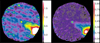 |
Fig. A.1 NIKA2 maps of IRAS 04370+2559 at 1.1 mm (left) and 2.0 mm (right) in mJy/pixel. The pixel size is 3″ and the data have been convolved to a FWHM resolution of 20″. |
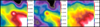 |
Fig. A.2 Simulation of the effect of the 2 mm noise on the data: zoom on the input 160-μm map (left), on the simulation output (middle) and on the difference between the two maps, with a smaller dynamic range (right). The pixel size and FWHM resolution are the same as in Fig. A.1 and the flux unit is Jy/pixel. |
Photometric information from the NIKA2 maps was gathered via aperture photometry. We used an aperture radius of 15″ and subtracted a local background estimated in an annulus between 30–50″, avoiding the extended emission associated with the bright source to the south-west (i.e., L 1527 IRS). We corrected these fluxes by aperture correction factors estimated from the above-mentioned Uranus observations. We arrived at the following flux densities:
![Mathematical equation: $\[\begin{aligned}& F_\nu(1.1 \mathrm{~mm})=58.2 ~\mathrm{mJy} \pm 2.4 ~\mathrm{mJy} \pm 3.5 ~\mathrm{mJy}, \\& F_\nu(2.0 \mathrm{~mm})=23.9 ~\mathrm{mJy} \pm 0.6 ~\mathrm{mJy} \pm 0.8 ~\mathrm{mJy}.\end{aligned}\]$](/articles/aa/full_html/2024/12/aa51981-24/aa51981-24-eq29.png)
The first error term is derived from the random noise in the photometry aperture via ![Mathematical equation: $\[\sigma_{\text {(flux density) }}=\sqrt{N_{\text {pix }}} \times \sigma_{\text {map }}\]$](/articles/aa/full_html/2024/12/aa51981-24/aa51981-24-eq30.png) , with Npix denoting the number of pixels in the aperture. The second term assumes formal uncertainties of 3.5% and 6.0% in the general flux calibration for 2.0 mm and 1.25 mm, respectively. These numbers are derived from the variations in the Uranus fluxes during the observing run containing our target observations and are in line with the typical values reported in Perotto et al. (2020).
, with Npix denoting the number of pixels in the aperture. The second term assumes formal uncertainties of 3.5% and 6.0% in the general flux calibration for 2.0 mm and 1.25 mm, respectively. These numbers are derived from the variations in the Uranus fluxes during the observing run containing our target observations and are in line with the typical values reported in Perotto et al. (2020).
References
- Adelman-McCarthy, J. K., et al. 2011, VizieR Online Data Catalog: The SDSS Photometric Catalog, Release 8 (Adelman-McCarthy+, 2011), VizieR On-line Data Catalog: II/306 [Google Scholar]
- Allard, F., Homeier, D., & Freytag, B. 2011, in Astronomical Society of the Pacific Conference Series, 448, 16th Cambridge Workshop on Cool Stars, Stellar Systems, and the Sun, eds. C. Johns-Krull, M. K. Browning, & A. A. West, 91 [Google Scholar]
- Andrews, S. M. 2020, ARA&A, 58, 483 [Google Scholar]
- Andrews, S. M., & Williams, J. P. 2005, ApJ, 631, 1134 [Google Scholar]
- Andrews, S. M., Wilner, D. J., Espaillat, C., et al. 2011, ApJ, 732, 42 [Google Scholar]
- Andrews, S. M., Rosenfeld, K. A., Kraus, A. L., & Wilner, D. J. 2013, ApJ, 771, 129 [Google Scholar]
- Andrews, S. M., Terrell, M., Tripathi, A., et al. 2018, ApJ, 865, 157 [Google Scholar]
- Ansdell, M., Williams, J. P., van der Marel, N., et al. 2016, ApJ, 828, 46 [Google Scholar]
- Avenhaus, H., Quanz, S. P., Garufi, A., et al. 2018, ApJ, 863, 44 [NASA ADS] [CrossRef] [Google Scholar]
- Babaian, D. 2020, Master Thesis, California State University, Northridge, USA [Google Scholar]
- Ballering, N. P., & Eisner, J. A. 2019, AJ, 157, 144 [Google Scholar]
- Baraffe, I., Homeier, D., Allard, F., & Chabrier, G. 2015, A&A, 577, A42 [NASA ADS] [CrossRef] [EDP Sciences] [Google Scholar]
- Barenfeld, S. A., Carpenter, J. M., Ricci, L., & Isella, A. 2016, ApJ, 827, 142 [Google Scholar]
- Birnstiel, T. 2023, arXiv e-prints [arXiv:2312.13287] [Google Scholar]
- Birnstiel, T., Dullemond, C. P., Zhu, Z., et al. 2018, ApJ, 869, L45 [CrossRef] [Google Scholar]
- Borucki, W. J., Koch, D., Basri, G., et al. 2010, Science, 327, 977 [Google Scholar]
- Bouwman, J., Henning, T., Hillenbrand, L. A., et al. 2008, ApJ, 683, 479 [NASA ADS] [CrossRef] [Google Scholar]
- Bruggeman, D. 1935, Ann. Phys., 416, 636 [NASA ADS] [CrossRef] [Google Scholar]
- Brunngräber, R., & Wolf, S. 2021, A&A, 648, A87 [NASA ADS] [CrossRef] [EDP Sciences] [Google Scholar]
- Cardelli, J. A., Clayton, G. C., & Mathis, J. S. 1989, ApJ, 345, 245 [Google Scholar]
- Cazzoletti, P., Manara, C. F., Liu, H. B., et al. 2019, A&A, 626, A11 [NASA ADS] [CrossRef] [EDP Sciences] [Google Scholar]
- D’Alessio, P., Calvet, N., Hartmann, L., Franco-Hernández, R., & Servín, H. 2006, ApJ, 638, 314 [Google Scholar]
- Dominik, C., & Tielens, A. G. G. M. 1997, ApJ, 480, 647 [Google Scholar]
- Dominik, C., Min, M., & Tazaki, R. 2021, OpTool: Command-line driven tool for creating complex dust opacities, Astrophysics Source Code Library [record ascl:2104.010] [Google Scholar]
- Draine, B. T. 2003, ARA&A, 41, 241 [NASA ADS] [CrossRef] [Google Scholar]
- Draine, B. T., & Flatau, P. J. 1994, J. Opt. Soc. Am. A, 11, 1491 [NASA ADS] [CrossRef] [Google Scholar]
- Draine, B. T., & Flatau, P. J. 2010, arXiv e-prints [arXiv:1002.1505] [Google Scholar]
- Dullemond, C. P., & Dominik, C. 2004, A&A, 421, 1075 [NASA ADS] [CrossRef] [EDP Sciences] [Google Scholar]
- Dullemond, C. P., Juhasz, A., Pohl, A., et al. 2012, Astrophysics Source Code Library [record ascl:1202.015] [Google Scholar]
- Eistrup, C., & Henning, T. 2022, A&A, 667, A160 [NASA ADS] [CrossRef] [EDP Sciences] [Google Scholar]
- Ejlali, G., Adam, R., Ade, P., et al. 2024, in European Physical Journal Web of Conferences, 293, 00016 [NASA ADS] [CrossRef] [EDP Sciences] [Google Scholar]
- Feiden, G. A. 2016, A&A, 593, A99 [NASA ADS] [CrossRef] [EDP Sciences] [Google Scholar]
- Feigelson, E. D., & Nelson, P. I. 1985, ApJ, 293, 192 [NASA ADS] [CrossRef] [Google Scholar]
- Fukagawa, M., Tamura, M., Itoh, Y., et al. 2010, PASJ, 62, 347 [NASA ADS] [Google Scholar]
- Gaia Collaboration (Vallenari, A., et al.) 2023, A&A, 674, A1 [NASA ADS] [CrossRef] [EDP Sciences] [Google Scholar]
- Garrod, R. T., & Herbst, E. 2006, A&A, 457, 927 [NASA ADS] [CrossRef] [EDP Sciences] [Google Scholar]
- Ginski, C., Tazaki, R., Dominik, C., & Stolker, T. 2023, ApJ, 953, 92 [NASA ADS] [CrossRef] [Google Scholar]
- Grant, S. L., Espaillat, C. C., Wendeborn, J., et al. 2021, ApJ, 913, 123 [NASA ADS] [CrossRef] [Google Scholar]
- Guerra-Alvarado, O. M., Carrasco-González, C., Macíasy, E., et al. 2024, A&A, 686, A298 [NASA ADS] [CrossRef] [EDP Sciences] [Google Scholar]
- Guidi, G., Isella, A., Testi, L., et al. 2022, A&A, 664, A137 [NASA ADS] [CrossRef] [EDP Sciences] [Google Scholar]
- Gullbring, E., Hartmann, L., Briceño, C., & Calvet, N. 1998, ApJ, 492, 323 [Google Scholar]
- Gupta, A., Miotello, A., Manara, C. F., et al. 2023, A&A, 670, L8 [NASA ADS] [CrossRef] [EDP Sciences] [Google Scholar]
- Gupta, A., Miotello, A., Williams, J. P., et al. 2024, A&A, 683, A133 [NASA ADS] [CrossRef] [EDP Sciences] [Google Scholar]
- Harsono, D., Bruderer, S., & van Dishoeck, E. F. 2015, A&A, 582, A41 [NASA ADS] [CrossRef] [EDP Sciences] [Google Scholar]
- Hartmann, L. 2009, Accretion Processes in Star Formation, 2nd edn [Google Scholar]
- Hendler, N. P., Mulders, G. D., Pascucci, I., et al. 2017, ApJ, 841, 116 [Google Scholar]
- Hendler, N., Pascucci, I., Pinilla, P., et al. 2020, ApJ, 895, 126 [Google Scholar]
- Henning, T., & Semenov, D. 2013, Chem. Rev., 113, 9016 [Google Scholar]
- Henning, T., & Stognienko, R. 1996, A&A, 311, 291 [NASA ADS] [Google Scholar]
- Hsieh, C.-H., Arce, H. G., José Maureira, M., et al. 2024, arXiv e-prints [arXiv:2404.02809] [Google Scholar]
- Isobe, T., Feigelson, E. D., & Nelson, P. I. 1986, ApJ, 306, 490 [Google Scholar]
- Jang, H., Waters, R., Kaeufer, T., et al. 2024, A&A, 691, A148 [NASA ADS] [CrossRef] [EDP Sciences] [Google Scholar]
- Jorda, L., Gaskell, R., Capanna, C., et al. 2016, Icarus, 277, 257 [Google Scholar]
- Juhász, A., Bouwman, J., Henning, T., et al. 2010, ApJ, 721, 431 [Google Scholar]
- Kataoka, A., Tanaka, H., Okuzumi, S., & Wada, K. 2013, A&A, 557, L4 [NASA ADS] [CrossRef] [EDP Sciences] [Google Scholar]
- Kirchschlager, F., & Wolf, S. 2013, A&A, 552, A54 [NASA ADS] [CrossRef] [EDP Sciences] [Google Scholar]
- Kirchschlager, F., & Wolf, S. 2014, A&A, 568, A103 [NASA ADS] [CrossRef] [EDP Sciences] [Google Scholar]
- Kirchschlager, F., Wolf, S., & Madlener, D. 2016, MNRAS, 462, 858 [CrossRef] [Google Scholar]
- Kirchschlager, F., Bertrang, G. H. M., & Flock, M. 2019, MNRAS, 488, 1211 [NASA ADS] [CrossRef] [Google Scholar]
- Kley, W., & Nelson, R. P. 2012, ARA&A, 50, 211 [Google Scholar]
- Kofman, W., Herique, A., Barbin, Y., et al. 2015, Science, 349, 2.639 [NASA ADS] [CrossRef] [Google Scholar]
- Krijt, S., Ciesla, F. J., & Bergin, E. A. 2016, ApJ, 833, 285 [Google Scholar]
- Lay, O. P., Carlstrom, J. E., & Hills, R. E. 1997, ApJ, 489, 917 [NASA ADS] [CrossRef] [Google Scholar]
- Liu, H. B. 2019, ApJ, 877, L22 [NASA ADS] [CrossRef] [Google Scholar]
- Liu, Y., Madlener, D., Wolf, S., Wang, H., & Ruge, J. P. 2012, A&A, 546, A7 [NASA ADS] [CrossRef] [EDP Sciences] [Google Scholar]
- Liu, Y., Henning, T., Carrasco-González, C., et al. 2017, A&A, 607, A74 [NASA ADS] [CrossRef] [EDP Sciences] [Google Scholar]
- Liu, Y., Dipierro, G., Ragusa, E., et al. 2019, A&A, 622, A75 [NASA ADS] [CrossRef] [EDP Sciences] [Google Scholar]
- Liu, Y., Linz, H., Fang, M., et al. 2022, A&A, 668, A175 [NASA ADS] [CrossRef] [EDP Sciences] [Google Scholar]
- Luhman, K. L., Allen, P. R., Espaillat, C., Hartmann, L., & Calvet, N. 2010, ApJS, 186, 111 [Google Scholar]
- Lynden-Bell, D., & Pringle, J. E. 1974, MNRAS, 168, 603 [Google Scholar]
- Macías, E., Guerra-Alvarado, O., Carrasco-González, C., et al. 2021, A&A, 648, A33 [EDP Sciences] [Google Scholar]
- Manara, C. F., Morbidelli, A., & Guillot, T. 2018, A&A, 618, L3 [NASA ADS] [CrossRef] [EDP Sciences] [Google Scholar]
- Manara, C. F., Ansdell, M., Rosotti, G. P., et al. 2023, in Astronomical Society of the Pacific Conference Series, 534, Protostars and Planets VII, eds S. Inutsuka, Y. Aikawa, T. Muto, K. Tomida, & M. Tamura, 539 [Google Scholar]
- Mayor, M., Marmier, M., Lovis, C., et al. 2011, arXiv e-prints [arXiv:1109.2497] [Google Scholar]
- Michoulier, S., Gonzalez, J.-F., & Price, D. J. 2024, A&A, 688, A31 [NASA ADS] [CrossRef] [EDP Sciences] [Google Scholar]
- Min, M., Canovas, H., Mulders, G. D., & Keller, C. U. 2012, A&A, 537, A75 [NASA ADS] [CrossRef] [EDP Sciences] [Google Scholar]
- Miotello, A., Kamp, I., Birnstiel, T., Cleeves, L. C., & Kataoka, A. 2023, in Astronomical Society of the Pacific Conference Series, 534, Protostars and Planets VII, eds. S. Inutsuka, Y. Aikawa, T. Muto, K. Tomida, & M. Tamura, 501 [Google Scholar]
- Mulders, G. D., Pascucci, I., Ciesla, F. J., & Fernandes, R. B. 2021, ApJ, 920, 66 [NASA ADS] [CrossRef] [Google Scholar]
- Natta, A., Testi, L., Calvet, N., et al. 2007, in Protostars and Planets V, eds. B. Reipurth, D. Jewitt, & K. Keil, 767 [Google Scholar]
- Öberg, K. I., Facchini, S., & Anderson, D. E. 2023, ARA&A, 61, 287 [CrossRef] [Google Scholar]
- Ohashi, N., Tobin, J. J., Jørgensen, J. K., et al. 2023, ApJ, 951, 8 [NASA ADS] [CrossRef] [Google Scholar]
- Okuzumi, S., Tanaka, H., Kobayashi, H., & Wada, K. 2012, ApJ, 752, 106 [NASA ADS] [CrossRef] [Google Scholar]
- Paardekooper, S., Dong, R., Duffell, P., et al. 2023, in Astronomical Society of the Pacific Conference Series, 534, Protostars and Planets VII, eds. S. Inutsuka, Y. Aikawa, T. Muto, K. Tomida, & M. Tamura, 685 [Google Scholar]
- Pascucci, I., Testi, L., Herczeg, G. J., et al. 2016, ApJ, 831, 125 [Google Scholar]
- Perotto, L., Ponthieu, N., Macías-Pérez, J. F., et al. 2020, A&A, 637, A71 [NASA ADS] [CrossRef] [EDP Sciences] [Google Scholar]
- Pinte, C., Padgett, D. L., Ménard, F., et al. 2008, A&A, 489, 633 [NASA ADS] [CrossRef] [EDP Sciences] [Google Scholar]
- Pinte, C., Dent, W. R. F., Ménard, F., et al. 2016, ApJ, 816, 25 [Google Scholar]
- Purcell, E. M., & Pennypacker, C. R. 1973, ApJ, 186, 705 [NASA ADS] [CrossRef] [Google Scholar]
- Rebull, L. M., Padgett, D. L., McCabe, C. E., et al. 2010, ApJS, 186, 259 [NASA ADS] [CrossRef] [Google Scholar]
- Ribas, Á., Espaillat, C. C., Macías, E., et al. 2017, ApJ, 849, 63 [NASA ADS] [CrossRef] [Google Scholar]
- Ricci, L., Testi, L., Natta, A., & Brooks, K. J. 2010, A&A, 521, A66 [NASA ADS] [CrossRef] [EDP Sciences] [Google Scholar]
- Rilinger, A. M., Espaillat, C. C., Xin, Z., et al. 2023, ApJ, 944, 66 [NASA ADS] [CrossRef] [Google Scholar]
- Roussel, H. 2013, PASP, 125, 1126 [Google Scholar]
- Savvidou, S., & Bitsch, B. 2024, A&A, submitted [arXiv:2407.08533] [NASA ADS] [CrossRef] [EDP Sciences] [Google Scholar]
- Schwarz, K. R., Calahan, J. K., Zhang, K., et al. 2021, ApJS, 257, 20 [NASA ADS] [CrossRef] [Google Scholar]
- Segura-Cox, D. M., Schmiedeke, A., Pineda, J. E., et al. 2020, Nature, 586, 228 [NASA ADS] [CrossRef] [Google Scholar]
- Semenov, D., Henning, T., Helling, C., Ilgner, M., & Sedlmayr, E. 2003, A&A, 410, 611 [NASA ADS] [CrossRef] [EDP Sciences] [Google Scholar]
- Sheehan, P. D., Tobin, J. J., Federman, S., Megeath, S. T., & Looney, L. W. 2020, ApJ, 902, 141 [Google Scholar]
- Sierra, A., & Lizano, S. 2020, ApJ, 892, 136 [Google Scholar]
- Skrutskie, M. F., Cutri, R. M., Stiening, R., et al. 2006, AJ, 131, 1163 [NASA ADS] [CrossRef] [Google Scholar]
- Stammler, S. M., Birnstiel, T., Panić, O., Dullemond, C. P., & Dominik, C. 2017, A&A, 600, A140 [NASA ADS] [CrossRef] [EDP Sciences] [Google Scholar]
- Stognienko, R., Henning, T., & Ossenkopf, V. 1995, A&A, 296, 797 [NASA ADS] [Google Scholar]
- Stolker, T., Dominik, C., Avenhaus, H., et al. 2016, A&A, 595, A113 [NASA ADS] [CrossRef] [EDP Sciences] [Google Scholar]
- Tazaki, R., Tanaka, H., Kataoka, A., Okuzumi, S., & Muto, T. 2019a, ApJ, 885, 52 [Google Scholar]
- Tazaki, R., Tanaka, H., Muto, T., Kataoka, A., & Okuzumi, S. 2019b, MNRAS, 485, 4951 [NASA ADS] [CrossRef] [Google Scholar]
- Tazaki, R., Ginski, C., & Dominik, C. 2023, ApJ, 944, L43 [NASA ADS] [CrossRef] [Google Scholar]
- Tazzari, M., Testi, L., Natta, A., et al. 2021, MNRAS, 506, 5117 [NASA ADS] [CrossRef] [Google Scholar]
- Thompson, S. E., Coughlin, J. L., Hoffman, K., et al. 2018, ApJS, 235, 38 [NASA ADS] [CrossRef] [Google Scholar]
- Tripathi, A., Andrews, S. M., Birnstiel, T., & Wilner, D. J. 2017, ApJ, 845, 44 [Google Scholar]
- Tychoniec, Ł., Tobin, J. J., Karska, A., et al. 2018, ApJS, 238, 19 [Google Scholar]
- Tychoniec, Ł., Manara, C. F., Rosotti, G. P., et al. 2020, A&A, 640, A19 [NASA ADS] [CrossRef] [EDP Sciences] [Google Scholar]
- Ueda, T., Kataoka, A., & Tsukagoshi, T. 2020, ApJ, 893, 125 [Google Scholar]
- Ueda, T., Tazaki, R., Okuzumi, S., Flock, M., & Sudarshan, P. 2024, Nat. Astron., 8, 1148 [NASA ADS] [CrossRef] [Google Scholar]
- Vaidya, D. B., & Gupta, R. 2011, A&A, 528, A57 [NASA ADS] [CrossRef] [EDP Sciences] [Google Scholar]
- van der Marel, N., Williams, J. P., Ansdell, M., et al. 2018, ApJ, 854, 177 [Google Scholar]
- van der Plas, G., Ménard, F., Ward-Duong, K., et al. 2016, ApJ, 819, 102 [NASA ADS] [CrossRef] [Google Scholar]
- Voshchinnikov, N. V., & Henning, T. 2008, A&A, 483, L9 [NASA ADS] [CrossRef] [EDP Sciences] [Google Scholar]
- Warren, S. G., & Brandt, R. E. 2008, J. Geophys. Res. (Atmos.), 113, D14220 [Google Scholar]
- Williams, J. P., & Cieza, L. A. 2011, ARA&A, 49, 67 [Google Scholar]
- Wolf, S., Schegerer, A., Beuther, H., Padgett, D. L., & Stapelfeldt, K. R. 2008, ApJ, 674, L101 [NASA ADS] [CrossRef] [Google Scholar]
- Wurm, G., & Blum, J. 1998, Icarus, 132, 125 [NASA ADS] [CrossRef] [Google Scholar]
- Xin, Z., Espaillat, C. C., Rilinger, A. M., Ribas, Á., & Macías, E. 2023, ApJ, 942, 4 [NASA ADS] [CrossRef] [Google Scholar]
- Ysard, N., Jones, A. P., Demyk, K., Boutéraon, T., & Koehler, M. 2018, A&A, 617, A124 [NASA ADS] [CrossRef] [EDP Sciences] [Google Scholar]
- Zhang, K., Booth, A. S., Law, C. J., et al. 2021, ApJS, 257, 5 [NASA ADS] [CrossRef] [Google Scholar]
- Zhang, S., Zhu, Z., Ueda, T., et al. 2023, ApJ, 953, 96 [NASA ADS] [CrossRef] [Google Scholar]
- Zhu, Z., Zhang, S., Jiang, Y.-F., et al. 2019, ApJ, 877, L18 [NASA ADS] [CrossRef] [Google Scholar]
When the particle sizes are in the Rayleigh limit, fluffy grains can have increased dust opacities at millimeter wavelengths compared to compact grains with the same mass, and the increase is highly dependent on the dust composition (e.g., Stognienko et al. 1995; Henning & Stognienko 1996).
All Tables
All Figures
|
Fig. 1 Dust properties considered in this work. Panel a: mass absorption coefficient at λ = 1.3 mm as a function of |
| In the text | |
|
Fig. 2 Comparison of F1.3mm (upper panel) and Tdust (bottom panel) between models that use compact dust opacities (black) and porous dust opacities (blue), respectively. In the models, all of other parameters are fixed: Rc = 30 AU, Ψ = 1.15, H100 = 10 AU. |
| In the text | |
|
Fig. 3 Dust temperature of a representative model with parameters of Mdust = 10−4 M⊙, Rc = 30 AU, Ψ = 1.15, and H100 = 10 AU. For a better representation, we show the quantity |
| In the text | |
|
Fig. 4 Statistics of the effective disk radius R68 from the model grid. Upper panel: ranges of R68 for each of the sampled Rc. The blue lines refer to the result when porous dust grains are considered, whereas the grey lines represent the case by using compact dust opacities. The thickness of lines is only for a better illustration. Bottom panel: relation between R68 and F0.88mm. The blue curve and grey curves enclose the regions occupied by the 9360 models with porous grains and compact grains, respectively. The dashed line shows the relation log R68 = 2.16 + 0.53 log F0.88mm (Hendler et al. 2020). The red dot indicates the expected position of IRAS 04370+2559 in the diagram; for details, see Sect. 4.2. |
| In the text | |
|
Fig. 5 Mass-averaged dust temperature as a function of stellar luminosity. The blue solid curve, expressed as log Tdust = 1.445 + 0.224 log L⋆ + 0.013 (log L⋆)2 is the best-fit relation to our models. The black dashed line refers to the relation Tdust = 25 (L⋆/L⊙)0.25 K presented by Andrews et al. (2013). The green dashed line shows the relation Tdust = 22 (L⋆/L⊙)0.16 K suggested by van der Plas et al. (2016). |
| In the text | |
|
Fig. 6 Dust masses in protoplanetary disks and their statistics. Upper panel: Mdust as a function of M⋆. Black symbols show the results derived by Manara et al. (2023), while blue symbols represent our calculations considering porous dust opacities and a Tdust − L⋆ scaling given by Eq. (6), see Sect. 3. Millimeter detections are indicated with dots, whereas triangles mean upper limits of the millimeter flux are reported. The dashed line depicts the value of 100·Mdust = 0.01·M⋆. Bottom panel: CDF of Mdust. The grey curve shows the result calculated with porous dust opacities and a constant dust temperature Tdust = 20 K. The red curve refers to the distribution of exoplanet masses obtained by Mulders et al. (2021). The vertical dashed lines mark the median values of each distribution. |
| In the text | |
|
Fig. 7 Fitting results of the IRAS 04370+2559 disk. Panel a: SEDs of IRAS 04370+2559. The best-fit radiative transfer models with compact dust opacities and porous dust opacities are shown with black lines and blue lines, respectively. The grey curve refers to the input BT-Settl spectrum, and photometric data points are overlaid with red dots. Panels b–e: Bayesian probability distributions for Log10(Mdust/M⊙), Log10(Rc/AU), H100, and Ψ. The triangles indicate the best-fit parameter values. The vertical dashed line in panel b marks the analytic dust mass calculated with Eq. (1) by assuming Tdust = 20 K and κ1.3mm = 2.3 cm2/g. |
| In the text | |
|
Fig. A.1 NIKA2 maps of IRAS 04370+2559 at 1.1 mm (left) and 2.0 mm (right) in mJy/pixel. The pixel size is 3″ and the data have been convolved to a FWHM resolution of 20″. |
| In the text | |
|
Fig. A.2 Simulation of the effect of the 2 mm noise on the data: zoom on the input 160-μm map (left), on the simulation output (middle) and on the difference between the two maps, with a smaller dynamic range (right). The pixel size and FWHM resolution are the same as in Fig. A.1 and the flux unit is Jy/pixel. |
| In the text | |
Current usage metrics show cumulative count of Article Views (full-text article views including HTML views, PDF and ePub downloads, according to the available data) and Abstracts Views on Vision4Press platform.
Data correspond to usage on the plateform after 2015. The current usage metrics is available 48-96 hours after online publication and is updated daily on week days.
Initial download of the metrics may take a while.