| Issue |
A&A
Volume 668, December 2022
|
|
|---|---|---|
| Article Number | A175 | |
| Number of page(s) | 18 | |
| Section | Interstellar and circumstellar matter | |
| DOI | https://doi.org/10.1051/0004-6361/202244505 | |
| Published online | 20 December 2022 | |
Underestimation of the dust mass in protoplanetary disks: Effects of disk structure and dust properties★
1
Purple Mountain Observatory & Key Laboratory for Radio Astronomy, Chinese Academy of Sciences,
10 Yuanhua Road,
Nanjing
210023, PR China
e-mail: This email address is being protected from spambots. You need JavaScript enabled to view it.
2
Max-Planck-Institut für Astronomie,
Königstuhl 17,
69117
Heidelberg, Germany
3
Institut für Theoretische Physik und Astrophysik, Christian-Albrechts-Universität zu Kiel,
Leibnizstr. 15,
24118
Kiel, Germany
4
School of Physics and Astronomy, University of Leicester,
Leicester
LE1 7RH, UK
5
Dipartimento di Fisica, Università degli Studi di Milano,
Via Giovanni Celoria, 16,
20133,
Milano, Italy
6
Leiden University,
Niels Bohrweg 2,
NL-2333 CA
Leiden, The Netherlands
7
School of Astronomy and Space Science, University of Science and Technology of China,
96 Jinzhai Road,
Hefei
230026, PR China
Received:
15
July
2022
Accepted:
13
October
2022
Abstract
The total number of dust grains in protoplanetary disks is one of the key properties that characterizes the potential for planet formation. With (sub-)millimeter flux measurements, literature studies usually derive the dust mass using an analytic formula under the assumption of optically thin emission, which may lead to a substantial underestimation. In this work, we conduct a parameter study with the goal of investigating the effects of disk structure and dust properties on the underestimation through self-consistent radiative transfer models. Different dust models, scattering modes, and approaches for dust settling are considered and compared. The influences of disk substructures, such as rings and crescents, on the mass derivation are investigated as well. The results indicate that the traditional analytic method can underestimate the mass by a factor of a few to several hundreds, depending on the optical depth along the line of sight set mainly by the true dust mass, disk size, and inclination. As an application, we performed a detailed radiative transfer modeling of the spectral energy distribution of DoAr 33, one of the disks observed by the Disk Substructures at High Angular Resolution Project (DSHARP). When the DSHARP dust opacities are adopted, the most probable dust mass returned from the Bayesian analysis is roughly seven times higher than the value given by the analytic calculation. Our study demonstrates that estimating disk dust masses from radiative transfer modeling is one solution to alleviate the problem of insufficient mass for planet formation that was raised in the era of the Atacama Large Millimeter/submillimeter Array.
Key words: circumstellar matter / protoplanetary disks / radiative transfer
Herschel is an ESA space observatory with science instruments provided by European-led Principal Investigator consortia and with important participation from NASA.
© Y. Liu et al. 2022
 Open Access article, published by EDP Sciences, under the terms of the Creative Commons Attribution License (https://creativecommons.org/licenses/by/4.0), which permits unrestricted use, distribution, and reproduction in any medium, provided the original work is properly cited.
This article is published in open access under the Subscribe-to-Open model. This email address is being protected from spambots. You need JavaScript enabled to view it. to support open access publication.
1 Introduction
Dust and gas material in protoplanetary disks are the building blocks of planetary systems. Within the timescale for disk dispersal, typically a few million years (Williams & Cieza 2011), micron-sized dust grains coagulate and grow by more than ten orders of magnitude until the assembly of large entities, such as pebbles and planetesimals (Testi et al. 2014; Birnstiel et al. 2016; Drazkowska et al. 2022). The gas-phase component either dissipates through a combination of complex mechanisms or can be captured by the growing giant planets (Balog et al. 2008; Machida et al. 2010; Ercolano & Pascucci 2017; Picogna et al. 2019; Pascucci et al. 2022). The total amount of material available in the disk plays a crucial role in determining whether planets can eventually form and what their nature is (e.g., Mordasini et al. 2012). The determination of protoplanetary disk masses can be accomplished through gas line or (sub-)millimeter continuum observations, although limitations exist for both diagnoses (Bergin & Williams 2017; Miotello et al. 2022).
Determining the disk gas mass is a difficult task, mainly because the most dominant component, H2, has no dipole moment, and it does not emit from the main disk mass reservoir. Carbon monoxide (CO) is an alternative tracer for gas masses. However, in addition to the requirement for a CO-H2 abundance ratio appropriate for protoplanetary disk environments, mass determinations from CO (and its isotopologs) lines need to be corrected for the effects of CO freeze-out in the cold midplane, which may be more effective than previously thought (Powell et al. 2022), and CO photodissociation in the hot surface layers as well as the isotope-selective processes (Williams & Best 2014; Miotello et al. 2014, Miotello et al. 2016). Hydrogen deuteride is believed to be a better probe, but to date, its J = 1−0 rotational transition line has been detected for only three disks with the Herschel/PACS spectrometer (Bergin et al. 2013; McClure et al. 2016).
Measuring dust continuum emission is less expensive than measuring gas line observations. With the advent of the Atacama Large Millimeter/submillimeter Array (ALMA), several nearby star formation regions have been surveyed, resulting in a large sample of disks (about 1000) with flux measurements at (sub-millimeter wavelengths (e.g., Ansdell et al. 2016; Barenfeld et al. 2016; Pascucci et al. 2016; Cazzoletti et al. 2019; Grant et al. 2021). Under optically thin conditions, (sub-)millimeter flux densities Fν can be converted into dust masses via the analytic equation
 (1)
(1)
where Bν(Tdust) refers to the Planck function given at the observed frequency ν and dust temperature Tdust, and the distance to the object is denoted as D. At a reference frequency of ν = 230 GHz (or wavelength λ ~ 1.3 mm), a value of 2.3 cm2 g−1 has frequently been adopted for the dust absorption opacity κν (e.g., Beckwith et al. 1990; Andrews et al. 2013). For the dust temperature, 20 K is a common choice. However, Andrews et al. (2013) suggested a stellar-luminosity (L*) dependent dust temperature Tdust = 25(L⋆/L⊙)0.25 K. The scaling of Tdust with L⋆ was further investigated for disks around low-mass stars and brown dwarfs (e.g., Daemgen et al. 2016; van der Plas et al. 2016; Hendler et al. 2017), and generally, the relation is found to be flatter than the prescription by Andrews et al. (2013).
A comparison between the statistic distribution of the analytic dust mass Mdust.ana and the minimum-mass solar nebula shows that only a few disks have enough material to produce our Solar System or its counterparts in the exoplanet population (e.g., Najita & Kenyon 2014; Manara et al. 2018; Andrews 2020; Mulders et al. 2021). Explanations for this discrepancy are generally provided by three different scenarios. The first scenario is that planet formation might be more efficient than what has been postulated, namely that in the evolutionary stage of the protoplanetary disk, dust grains have already grown up to pebbles, planetesimals, or even planetary embryos that are insensitive to (sub-)millimeter observations (e.g., Tychoniec et al. 2020). Supporting evidence is the prevalence of disk substructures, such as rings and gaps (e.g., ALMA Partnership 2015; Long et al. 2018; Andrews et al. 2018a), even in protostellar disks with relatively young ages (Segura-Cox et al. 2020; Sheehan et al. 2020). These fine-scale features are likely created by (proto-)planets that are still embedded in their natal disk (Kley & Nelson 2012). In the second scenario, the disk acts as a conveyor belt that transports material from the environment to the central star (Manara et al. 2018). Thus, the disk is replenished with material from the surrounding remnant envelope, part of which can contribute to the formation of planets. The third proposal concerns the reliability of mass estimation from Eq. (1), which is based on an optically thin assumption. Detailed radiative transfer analyses of millimeter data have demonstrated that protoplanetary disks, particularly in the inner regions, are not necessarily optically thin at millimeter wavelengths (e.g., Wolf et al. 2008; Pinte et al. 2016; Liu et al. 2019; Ueda et al. 2020). The measured fluxes only reflect dust material residing above the τ = 1 surface. Consequently, the calculated Mdust.ana is merely a lower limit. This underestimation has indeed been found in previous studies, but mostly for a limited number of objects (e.g., Maucó et al. 2018; Ballering & Eisner 2019; Carrasco-González et al. 2019; Ribas et al. 2020; Villenave et al. 2020; Macías et al. 2021; Guidi et al. 2022). Because the optical depth along the line of sight increases with the viewing angle, the analytic dust mass is expected to further deviate from the true dust mass of disks with high inclinations.
Moreover, deriving dust masses using Eq. (1) does not take into account the dust density distribution in the disk. The accumulating ALMA data show that in some cases, dust grains are quite highly concentrated within substructures such as rings and crescents. Examples are the disks around Oph IRS 48 (van der Marel et al. 2013), HD143006 (Pérez et al. 2018), HD 135344B (Cazzoletti et al. 2018), and MWC758 (Dong et al. 2018). Whether and to which level these configurations affect the mass estimation is unclear. In addition to a direct impact of dust opacities (therefore dust emissivities at millimeter wavelengths) on the mass determination, the choice for the dust model will also influence the resulting dust temperature, which in turn affects the mass determination. This parameter coupling is not considered in Eq. (1). In this work, using self-consistent radiative transfer models, we performed a detailed parameter study with the goal of systematically evaluating the extent of dust mass underestimation and its dependence on the disk structure and dust properties. The setup of the fiducial model and the method we used to quantify the mass underestimation are described in Sect. 2. In Sect. 3, effects of various model parameters and assumptions on the results are investigated. As an application, we model the spectral energy distribution (SED) of the DoAr 33 disk in Sect. 4. The paper concludes with a summary in Sect. 5.
Parameters of the fiducial model.
2 Fiducial disk model
In this section, we devise a fiducial radiative transfer model and introduce the method we used to quantify the degree of underestimation of the dust mass. Starting from the fiducial model, we can alter the assumption and thus investigate the effects of various parameters on the result. The well-tested code RADMC-3D1 was invoked to conduct the radiative transfer simulation (Dullemond et al. 2012). Table 1 gives an overview of parameters together with the values we adopted to describe the fiducial model.
2.1 Dust density distribution
We employed a flared disk surrounding a T Tauri star with stellar luminosity and temperature of L⋆ = 0.92 L⊙ and Teff = 4000 K. The disk was assumed to be passively heated by stellar irradiation. The dust density was assumed to follow a Gaussian vertical profile,
![Mathematical equation: $\rho (R,z,a) = {{\sum (R,a)} \over {\sqrt {2\pi } h(R,a)}}\exp \left[ { - {1 \over 2}{{\left( {{z \over {h(R,a)}}} \right)}^2}} \right],$](/articles/aa/full_html/2022/12/aa44505-22/aa44505-22-eq3.png) (2)
(2)
where R is the radial distance from the central star measured in the disk midplane. The surface density is described as a power law,
 (3)
(3)
with the proportionality factor Σ0(a) determined by normalizing the mass of dust grains in a certain grain size (a) bin. We set the disk inner radius Rin to 0.1 AU, which is close to the dust sublimation radius. The outer disk radius Rout was chosen to be 100 AU, meaning that we truncated the disk at Rout.
Theoretical studies showed that dust grains gradually decouple from the underlying gas distribution and tend to settle toward the midplane (Dullemond & Dominik 2004). This process has been confirmed by high-resolution observations, in which millimeter dust grains are found to be confined within scale heights of an order of a few AU (e.g., Gräfe et al. 2013; Pinte et al. 2016; Villenave et al. 2020), which is smaller than the typical gas pressure scale height (> 10 AU, Law et al. 2021; Rich et al. 2021). To account for dust settling, we assumed that the dust scale height h varies with R and the grain size a
 (4)
(4)
where β is the flaring index, and H100(a) stands for the scale height for a certain grain size at R = 100 AU. Using a power law, we parameterized the reference dust scale height as
 (5)
(5)
The parameter  denotes the scale height of the smallest dust grains that are expected to be well coupled with the gas. The quantity ξ is used to characterize the degree of dust settling. This simple prescription of dust settling has been used for multiwave-length modeling of protoplanetary disks (Pinte et al. 2008; Liu et al. 2017). We included 32 grain size bins that were logarithmically distributed from a fixed minimum grain size amin = 0.01 µm to a maximum grain size amax. The radiative transfer was performed using these 32 grain sizes as 32 different dust species, each of which has its own dust opacity (see Sect. 2.2). Moreover, they are assumed to be thermally decoupled in RADMC-3D. For the fiducial model, we adopted amax = 1 mm. The scale height for each of the 32 grain sizes is described by Eqs. (4) and (5). Given ξ = 0.14 and
  for the fiducial model, the scale height of the 1 mm dust grain equals 2 AU, which is consistent with observational constraints (Pinte et al. 2016; Villenave et al. 2020; Liu et al. 2022). When the dust and gas are perfectly mixed, ξ = 0, and
  becomes independent of the grain size and is equal to the gas scale height, the disk is the well-mixed case.
The fraction of dust mass in each grain size bin is calculated via
 (6)
(6)
where a0 = exp[ln(aj) − ∆/2], a1 = exp[ln(aj) + ∆/2], alower = exp[ln(amin) − ∆/2], aupper = exp[ln(amax) + ∆/2], and ∆ is the step width in the logarithmic scale used to sample the 32 grain sizes. The vertically integrated grain size distribution is assumed to be n(a) ∝ a−3.5, and ρgrain is the bulk density of the dust ensemble. This means that when the total dust mass (Mdust) in the entire disk is given, we know the dust mass for each grain size bin, and therefore can derive the proportionality factor Σ0(a) in Eq. (3). Figure 1 shows the vertical density profile of the fiducial model at a radius of R = 10 AU for three representative grain sizes.
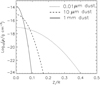 |
Fig. 1 Vertical density profile of the fiducial model at a radius of R = 10 AU. The model includes 32 grains sizes logarithmically spaced from amin = 0.01 µm to amax = 1 mm. The results are shown here for dust grains with three representative sizes, i.e., 0.01 µm (dotted line), 10 µm (dashed line), and 1 mm (solid line). |
2.2 Dust properties
For the dust composition, we used the model by Birnstiel et al. (2018), which is composed of water ice, astronomical silicates, troilite, and refractory organic material, with volume fractions being 36%, 17%, 3%, and 44%, respectively. The bulk density of the dust mixture is ρgrain = 1.675 g cm−3. This dust model was used to interpret the ALMA data from the Disk Substructures at High Angular Resolution Project (DSHARP, Andrews et al. 2018a). We used the Mie theory to calculate the mass absorption and scattering coefficients for the sampled 32 grain sizes. The solid blue line in Fig. 2 shows the absorption coefficient at λ = 1.3 mm as a function of grain size. There are clear fluctuations for a ~ 0.2–0.7 mm due to the resonances when the size of the particle is comparable to λ/2π. The horizontal dashed line indicates the value of 2.3 cm2 g−1.
Dust scattering is expected to significantly affect the emission level and millimeter spectral index of optically thick disks (Zhu et al. 2019; Liu 2019). Consequently, whether or not this mechanism is taken into account will influence the inferred dust temperature, optical depth, dust mass, and grain size; see Appendix C of Carrasco-González et al. (2019), for instance. We switched on isotropic scattering in both the thermal Monte Carlo simulation in which we computed the dust temperature and in the subsequent step to generate the SED. A more realistic treatment for dust scattering is considered and compared in Sect. 3.2.
Multiwavelength observations have shown that millimeter spectral slopes differ among disks even in the same star formation region (e.g., Ricci et al. 2010; Pinilla et al. 2017; Andrews 2020). The scatter of the observed millimeter spectral slopes can be attributed to different levels of dust processing or to different optical depths. Without a detailed analysis of multiwavelength data, the grain size distribution is not known, which could have a direct impact on the mass determination with Eq. (1). Moreover, the composition of dust grains is also found to vary for different disks (e.g., Juhász et al. 2010). Therefore, we also considered another dust model that was introduced in the DiscAnalysis project (DIANA, Woitke et al. 2016), and investigated the influence of a different choice for dust properties on the result; see Sect. 3.4.
 |
Fig. 2 Mass absorption coefficient κν at λ = 1.3 mm as a function of grain size a. The blue line shows the result by using the DSHARP dust model, and the case for the DIANA dust model is indicated with the black line. The horizontal dashed line marks the value of 2.3 cm2 g−1 that is commonly adopted to derive the analytic dust mass Mdust.ana in the literature. |
2.3 Properties of the fiducial model
The upper panel of Fig. 3 shows the dust density distribution of the fiducial model. The blue curve indicates the location of the τ1.3 mm = 1 surface considering that the disk is viewed at i = 41.8°. Within R ≲ 40 AU, disk interior layers are optically thick. We ran the thermal Monte Carlo simulation using 3 × 10⁷ photons in order to obtain a smooth temperature structure. The SED of the fiducial model was simulated and scaled to the distance of 140 pc, which is indicated as the blue line in the bottom panel of Fig. 3.
The midplane dust temperature ranges from ~1300K to ~ 10 K, roughly following a power law Tmidplane ∝ R−0.5. To give a representative dust temperature characterizing millimeter continuum emission, we calculated the mass-averaged dust temperature via
 (7)
(7)
where mdust(i, j) and tdust(i, j) are the dust mass and temperature in each cell (i) for each grain size (j), respectively. Similarly, we derived the mass-averaged dust opacity from
 (8)
(8)
where κν(i, j) are the dust opacity in each cell for each grain size. The fiducial model features a Tdust = 16.3 K (see Table 2) and  .
.
The simulated flux density at λ = 1.3 mm is Fν = 80.7 mJy. Because Fν, Tdust, and  of the fiducial model are exactly known, we can use Eq. (1) to derive a corresponding analytic dust mass required to produce the same amount of continuum in the optically thin regime. This gives us Mdustana = 2.2 × 10⁻⁴ M⊙. The true dust mass imported into the fiducial model is Mdust = 3 × 10⁻⁴ M⊙. We define the degree of mass underestimation as
 (9)
(9)
where the subscript is used to state that the calculation is based on 1.3 mm flux densities. Similar factors can be derived using data points at other wavelengths. The difference between Mdust and Mdust.ana basically reflects dust material hidden below the τ = 1 surface (see Fig. 3) because uncertainties on the dust temperature and opacity are eliminated in our definition.
 |
Fig. 3 Properties of the fiducial model with parameters given in Table 1. Upper panel: 2D dust density distribution. The blue and black lines draw the contour of τ1.3 mm = 1 when the disk is viewed at i = 41.8°, and the lines include the DSHARP and DIANA dust opacities, respectively. Bottom panel: model SEDs when the DSHARP (blue line) or DIANA (black line) opacities are adopted in the simulation. The dashed curve stands for the input photospheric spectrum with Teff = 4000 K, assuming log g = 3.5 and solar metallicity (Kurucz 1994). |
Comparison of results between models with isotropic and anisotropic scattering.
3 Effects of model parameters and assumptions on the results
3.1 Effects of model parameters
With the method we used to quantify the underestimation factor outlined in Sect. 2.3, we then changed the values for each model parameter to investigate their effects on the results. Parameters considered in the exploration were Rin, Rout, γ, Mdust,  , β, H100(1mm dust), or equivalent to ξ, amax, and i. Calculation of the underestimation factor always uses the mass-averaged dust opacity and temperature of the corresponding model. Figure 4 shows the flux densities at 0.88 mm and 1.3 mm, the mass-averaged temperature, and the underestimation factors.
Although the stellar properties were fixed, there clearly is a broad range for the mass-averaged temperature. Particularly the variation in Tdust with Rout can be up to a factor of 4, from ~32K for compact disks with Rout = 20 AU to ~8 K for large disks with Rout = 800 AU. Of the nine parameters, only Rin, aamax, and i have minor impacts on Tdust. A simple assumption of the temperature according to Tdust = 25 (L⋆/L⊙)0.25 = 24.5 K will therefore lead to differences in the determination of Mdust.ana.
The underestimation factor Λ ranges from a few to several hundreds. Higher dust masses and inclinations or smaller disk sizes result in the greatest underestimation in the dust mass because they work together to achieve a higher optical depth along the line of sight. Other parameters that aggravate the underestimation include smaller Rin, steeper γ, and lower β and aamax, which yields a higher κ. As the optical depth decreases with increasing wavelength, underestimations calculated based on 1.3 mm fluxes are systematically lower than those derived using the 0.88 mm fluxes. Long-wavelength observations are therefore required to better probe the dust mass in protoplanetary disks. The dashed red lines in Fig. 4 show the underestimation factors Λ1.3 mm that were calculated by assuming a constant κ1.3 mm = 2.3 cm2 g−1 and Tdust = 25(L⋆/L⊙)0.25 = 24.5K (hotter than most of the models). They are generally higher than those obtained by using the mass-averaged dust opacity and temperature of the models. This directly demonstrates the importance of taking disk structure and dust properties into account in the task of mass estimation.
Figures A.1 and A.2 show the variation in Λ with different model parameters when the disk is viewed at two extreme inclinations, that is, i = 0° (face on) and i = 90° (edge-on). The behavior of face-on disks is quite similar to that of the fiducial inclined disks. For edge-on disks, the underestimation factor becomes more sensitive to most of the explored parameters. This tendency can be clearly identified from the Λ − Rout, Λ − Mdust, Λ − H100(1 mm dust), and Λ − amax profiles. As a consequence, the mass determination for edge-on disks is more difficult than for disks with low inclinations because the accuracy of the result highly depends on how well many other parameters are constrained.
3.2 Effects of the dust-scattering mode
When dust grains grow up to millimeter sizes, the scattering coefficients at millimeter wavelengths become significantly larger than the absorption coefficients, resulting in a very high albedo. For instance, the albedo of the fiducial dust model is 0.9 at 1.3 mm. In this case, scattering of thermal reemission radiation on the SED should be taken into account. Theoretical studies have found that dust scattering can considerably reduce the emission from optically thick regions, with the reduction level depending on the inclination (e.g., Zhu et al. 2019; Sierra & Lizano 2020). Thus, an optically thick disk with scattering can be misidentified as an optically thin disk when scattering is ignored.
We compared the models when different modes of dust scattering were turned on. The results are summarized in Table 2. The difference in dust temperature between isotropic and anisotropic scattering models is merely ~0.5 K, regardless of the total dust mass (hence, intrinsic optical thickness). Anisotropic scattering always yields stronger emission. However, the flux discrepancy between the two modes does not exceed 16%, with larger differences generally found for more massive or more inclined disks. Therefore, when dust scattering is included, it does not significantly affect the underestimation factor.
3.3 Effects of the dust-settling approach
We also considered different approaches for dust settling. Dust settling basically determines the millimeter dust scale height. In the fiducial model, we used only three free parameters ( , ξ, and β) to parameterize the scale height; see Eqs. (4) and (5). The scale height of 1 mm dust grain is indicated as the blue line in Fig. 5. Theoretically, the vertical distribution of dust grains is a consequence of equilibrium between dust settling and vertical stirring induced by turbulent motions. Therefore, the scale heights of dust grains with different sizes are related to the turbulence strength αturb
 (10)
(10)
where  is the Stokes number (e.g., Dubrulle et al. 1995; Schräpler & Henning 2004; Woitke et al. 2016; Birnstiel et al. 2016). Because the smallest dust grain (0.01 µm in our case) is expected to be well mixed with the gas, we assumed that the gas pressure scale height Hgas follows
 (11)
(11)
This settling approach has four free parameters:  ,αturb, β, and the gas surface density Σgas. For Σgas, we simply scaled the dust surface density by a constant gas-to-dust mass ratio of 100. For αturb, we considered 3 × 10⁻⁴ and 3 × 10⁻³, which are consistent with observational constraints from gas line observations (e.g., Flaherty et al. 2017, 2020; Teague et al. 2018). The αturb/St ratios for the 0.2mm dust grain calculated at R ~ 80 AU are ~0.03 and ~ 0.3 for αturb = 3 × 10⁻⁴ and 3 × 10⁻³, respectively. These ratios are comparable with the results derived from analyzing the widths of dust rings in several DSHARP disks (Dullemond et al. 2018). The dust scale heights are shown with the black and red lines in Fig. 5. The model with αturb = 3 × 10⁻³ features a larger scale height than the fiducial setup across the entire radius. Consequently, it has a higher temperature and emits more continuum (see Table 3). A weaker turbulence of 3 × 10⁻⁴ makes the disk cooler and fainter, and now Tdust and F1.3 mm are comparable with those of the fiducial model.
In Table 3, we also provide the results when dust grains and gas are well coupled, which can be considered as a limiting case of the fiducial settled disk. When the settling degree ξ (see Eq. (5)) tends towards zero, the settled disk model turns into the well-mixed case and becomes the brightest at millimeter wavelengths among the models under comparison. It is naturally understood that when well-mixed radiative transfer models are used to fit observed SEDs, the lowest number of dust grains is required. Hence, dust mass determinations from radiative transfer analysis based on the well-mixed assumption are probably still lower limits.
 |
Fig. 4 Effects of model parameters on the results. Top row: flux densities at 0.88 and 1.3 mm (F0.88 mm and F1.3 mm, on the left Y-axis) and mass-averaged dust temperature (Tdust, on the right Y-axis) as a function of different model parameters. Bottom row: underestimation factor (Λ0.88 mm and Λ1.3 mm) as a function of different model parameters. When one particular parameter was explored, all the remaining parameters were fixed to their fiducial values listed in Table 1. The red dashed lines show the underestimation factors Λ1.3 mm that were calculated by assuming a constant Tdust = 25 (L⋆/L⊙)0.25 = 24.5 K and κ1.3 mm = 2.3 cm2 g−1. |
3.4 Effects of dust properties
To investigate how the dust properties affect the results, we used the standard dust properties introduced by the DIANA project (Woitke et al. 2016). The dust grains consist of 60% silicate (Mg0.7Fe0.3SiO3, Dorschner et al. 1995), 15% amorphous carbon (BE–sample, Zubko et al. 1996), and 25% porosity. These percentages are volume fractions that are used to derive the effective refractory indices by applying the Bruggeman mixing rule (Bruggeman 1935). Porous grains were considered because porosity, and its evolution during the collisional growth, helps to overcome the radial-drift barrier (e.g., Ormel et al. 2007; Garcia & Gonzalez 2020). We assumed a distribution of hollow spheres with a maximum hollow volume ratio of 0.8, and calculated the opacities using the OpacityTool package (Toon & Ackerman 1981; Min et al. 2005).
The black line in Fig. 2 shows κ1.3 mm as a function of grain size. The DIANA dust absorption coefficients are systematically larger than the DSHARP values. The choice for the material termed “organic” in the DSHARP model has a significant impact on the absorption coefficient; see Appendix B in Birnstiel et al. (2018). When we used the amorphous carbon (BE-sample; Zubko et al. 1996) instead, the absorption coefficients increased by a factor of ~5. The SEDs using different dust opacities are compared in the lower panel of Fig. 3, with F1.3 mm = 165.2 mJy and 80.7 mJy for the DIANA and DSHARP dust being imported, respectively. Models using the DIANA opacity are generally hotter, but the differences in the mass-averaged temperature are within ~2 K, even for very massive disks; see Fig. 6. Because the disk is more optically thick when the DIANA dust model is adopted, the underestimation factors are correspondingly systematically higher, as shown in Fig. 6.
 |
Fig. 5 Scale height of 1 mm dust as a function of R. The blue line shows the fiducial model with the dust settling prescribed by Eq. (5). The black and red lines stand for models when dust settling is parameterized according to Eq. (10) under different turbulence strengths αturb. |
Comparison of models using different prescriptions for dust settling.
 |
Fig. 6 Comparison of Λ1.3 mm (squares) and Tdust (filled circles) between models that use the DSHARP (blue symbols) and DIANA (black symbols) dust opacities in the simulation, respectively. Details can be found in Sect. 3.4. |
3.5 Effects of disk substructures
In the above modeling procedure, dust surface densities were assumed to follow a smooth power law, without sharp density fluctuations; see Eq. (3). However, high-resolution multiwave-length observations have revealed that many protoplanetary disks possess rings and crescents (e.g., van Boekel et al. 2017; Avenhaus et al. 2018; Fedele et al. 2018; Long et al. 2018; Andrews et al. 2018a; Cieza et al. 2021), which are thought to be a favorable place for planet formation (Andrews 2020). In some cases, these substructures, even located at large radial distances from the host central star, appear to be very bright in the millimeter continuum, indicating that a large number of dust grains are concentrated (e.g., ALMA Partnership 2015; Pérez et al. 2018; Dong et al. 2018; Cazzoletti et al. 2018).
The overdensities in disk substructures will increase the optical depth locally, which can in principle affect the mass determination. Detailed radiative transfer analysis confirms that some substructures are optically thick at ALMA wavelengths (e.g., Pinte et al. 2016; Liu et al. 2017, 2022; Ohashi & Kataoka 2019; Sierra et al. 2021). In order to investigate how the redistribution of dust grains in disks with substructures affects the mass determination, we considered four scenarios: one ring, two rings, three rings, and three rings plus a crescent. The surface densities of the substructures are defined as
 (12)
(12)
 (13)
(13)
where Rring or Rcres refers to the radial location of the feature, and σring or  stands for the radial width. For the crescent, θcres and
  were used to control the location and width in the azimuthal direction. The proportionality constant was set to be three times larger than that for the rings, under which the crescent can feature a high millimeter flux contrast to its neighboring ring. Table 4 lists the adopted parameter values. These values were chosen to be representative among the results that were derived by analyzing the brightness profiles of rings or crescents revealed by ALMA (e.g., Long et al. 2018; Huang et al. 2018; Pérez et al. 2018). When all the features are included, integrating Eqs. (12) and (13) results in mass fractions of 8%, 28%, 50%, and 14% for the first, second, and third ring and for the crescent, respectively.
We therefore gradually increased Mdust to let the substructures become optically thick. Dust opacities and settling approach were kept to the fiducial assumptions. The results for each scenario are presented in Fig. 7. We found that the tendencies of F1.3 mm, Tdust, and the overall level of Λ1.3 mm are generally similar to those for smooth disks. The maximum underestimation is achieved when the innermost ring alone is introduced. In this case, dust grains are confined within the smallest disk radius. When the outer substructures are added, the underestimation becomes less severe. This effect is mainly driven by the actual Rout. In other words, Rout has a stronger influence on the mass underestimation than the presence or absence of substructures. In order to validate the hypothesis, we ran additional simulations for smooth disks. The surface densities for R ≤ Rf were all fixed to the surface density at R = Rf, where Rf is the location of the outermost substructure (e.g., Rf = 65 AU for the case of three rings; see Table 4), and for R > Rf, we set the surface densities according to Eq. (12). In the case of three rings plus a crescent, we set the surface densities for R > Rf according to an azimuthally averaged profile described by a combination of Eqs. (12) and (13). In this case, the dust surface density does not vary within Rf (i.e., no rings, gaps, or crescent), and follows the same profile as for the disk with substructures in the outermost region, which would lead to an equivalent Rout. The filled green circles shown in the right column of Fig. 7 refer to the underestimation factors, which are similar to those of the disks with substructures.
Ring and crescent parameters.
4 Application to the DoAr 33 disk
We have shown that due to the optical depth effect, calculating disk dust masses using the analytic approach can lead to substantial underestimation, even when the dust temperature (Tdust) and opacity (κ) are known. The disk outer radius (Rout), inclination (i), and true dust mass (Mdust) are most important to create these optically thick regions. Fortunately, Rout and i can be derived from high-resolution (sub-)millimeter images that are available for a large number of disks through ALMA today. In this section, we conduct a detailed radiative transfer modeling of the SED for DoAr 33 in order to constrain the total dust mass in the disk. We then compare the result with the analytic dust mass.
4.1 DoAr 33 and its SED
DoAr 33 is a T Tauri star located in the Ophiuchus star formation region at a distance of 140 pc (Gaia Collaboration 2018). The spectral type K5.5 derived by Wilking et al. (2005) translates into an effective temperature of 4160 K using the SpT − Teff conversion reported by Herczeg & Hillenbrand (2014). To compile the SED, we collected data points at various wavelengths from the literature. Through the Chinese Telescope Access Program, we also conducted new CSO/SHARCII observations at 350 µm; see Appendix B for details about the observations and data reduction. Herschel photometry for DoAr 33 in the literature shows a surprisingly steep decline toward submillimeter wavelengths (Rebollido et al. 2015). Therefore, we re-reduced the Herschel/PACS and SPIRE data and performed the photometry based on a point-spread function fitting; see Appendix C. These efforts allowed us to build the SED with an excellent wavelength coverage. The measurements from optical to millimeter domains are summarized in Table 5, and they are shown with red dots in panel (a) of Fig. 8. Fitting the optical photometry with the Kuгucz atmosphere models yields a stellar luminosity of L⋆ = 0.97 L⊙.
4.2 Large grid of radiative transfer model SEDs
As one of the 20 disks selected in the DSHARP project, DoAr 33 was observed by ALMA with an angular resolution of ~35 mas (Andrews et al. 2018a). The disk is inclined by i = 41.8° and appears to be smooth in the 1.3 mm continuum image. Huang et al. (2018) defined the outer boundary of the millimeter disk to be the radius at which the enclosed flux is equal to 95% of the total flux. This is 27 AU, which means that DoAr 33 is the smallest of the 18 single-star disk systems targeted by DSHARP. We checked the 12CO J = 2−1 line data and found that the emission of 12CO is more extended, with a 95% enclosing flux radius of 70 AU. A more compact millimeter dust disk than the CO disk has also been found for other targets (e.g., Ansdell et al. 2018; Long et al. 2022), and it can naturally be explained by radial drift of dust particles (Trapman et al. 2019; Toci et al. 2021).
We built a large grid of radiative transfer models for DoAr 33. The model configuration is a slight variant of the fiducial setup. Dust grains with sizes ranging from amin = 0.01 µm to 10 µm are assumed to be distributed from 0.1 AU to 70 AU. Larger dust grains (i.e., a > 10 µm) have already drifted to the location where the DSHARP continuum data probes, and therefore, we truncated them at R = 27 AU. For the most interesting parameter Mdust, we sampled 13 grid points that are logarithmically distributed from 3 × 10⁻⁶ to 3 × 10⁻³ M⊙. For amax, we took 7 logarithmically spaced points from 0.1 mm to 100 mm. There are 8 points for  linearly spaced between 4 and 18 AU, and 9 linear points for β from 1.05 to 1.25. For the power-law index (γ) of the surface density, we chose a value of 0.5, which is close to the slope of the power law that was used to fit the azimuthally averaged surface brightness of the DSHARP image. Parameters not mentioned here were fixed to the fiducial values; see Table 1. In total, there are 6552 models in the grid, and we separately ran the simulation with the DSHARP and DIANA dust opacities.
4.3 Result and discussion
The best-fit model SEDs, identified as those with the lowest reduced χ2, are shown in panel a of Fig. 8. Following the procedure described in Pinte et al. (2008), a Bayesian analysis was conducted by using the 6552 SED models and assuming flat priors because there is no preliminary information about the parameters. The resulting marginalized probability distributions are presented in panels b−e of Fig. 8. The triangles indicate the parameter values of the best-fit radiative transfer model, all of which are less than one bin away from the most probable values. The relatively wide distribution of the probabilities, especially for amax, implies that there are degeneracies between model parameters in fitting the SED. The most probable dust masses are Mdust.RT = 3× 10⁻⁴(9.5× 10⁻⁵, 1.7× 10⁻³) and 9.5 × 10⁻⁵ M⊙ (5.3 × 10⁻⁵, 5.3 × 10⁻⁴) when the DSHARP and DIANA dust opacities are used, respectively, where the numbers given in parenthesis correspond to the 68% confidence interval. To calculate the analytic dust mass Mdust.ana, we adopted κ1.3 mm = 2.3 cm2 g−1 and Tdust = 25 (L⋆/L⊙)0.25 = 24.8 K for consistency with literature studies. We took the integrated flux of 35 mJy from the DSHARP project (see Table 5), and derived Mdust.ana = 4.1 × 10⁻⁵M⊙, which is indicated with the vertical dotted line in panel (b) of Fig. 8. The dust masses from radiative transfer modeling are 7.3 and 2.3 times higher than the analytic dust mass when the DSHARP and DIANA dust opacities were adopted in the simulation, respectively.
We take the most probable model that includes the DSHARP opacity as an illustration. Reg ions below the τ1.3 mm = 1 surface occupy ~70% of the total mass, which partly explains the large difference between Mdust.ana and Mdust.RT. The mass-averaged dust temperature is Tdust = 19.6 K, which is cooler than the analytic dust temperature 24.8 K. This also contributes to the mass difference. To reproduce the shallow millimeter spectral slope αmm = 2.1, the most probable maximum grain size is amax = 32 mm, yielding an absorption coefficient of  . The discrepancy in κ1.3 mm accounts for a difference of a factor of 2.3/0.7 = 3.3 in the dust mass. The millimeter spectral slope of DoAr 33 is typically found in other disks around both brown dwarfs (BDs) and T Tauri/Herbig stars (e.g., Ricci et al. 2010, 2014; Pinilla et al. 2017), implying that dust grains have grown to millimeter sizes at least. A multiwavelength analysis, such as the self-consistent radiative transfer modeling implemented in this study, is necessary to recover the grain size distribution, which is very important to characterize dust emis-sivities, and thus obtain a reliable determination of dust masses. This information is basically missing in the traditionally analytic approach.
The large underestimation of the dust mass obtained for DoAr 33 may not be a peculiarity of that source. With a thorough analysis of millimeter observations, Macías et al. (2021) recovered 4.5–5.9 times more mass for the TW Hydrae disk than with the usual analytic method. Similar underestimation factors have also been found for some disks in the Taurus star formation region (Ballering & Eisner 2019; Ribas et al. 2020). To give a rough assessment of how frequently a large underestimation would be encountered, Fig. 9 shows Λ1.3 mm and Tdust as a function of F1.3 mm and Rout. When we created the plot, we included models in which only Mdust and Rout were varied, because as discussed in Sect. 3.1, they have the most significant impact on the underestimation factor. Other parameters including the disk inclination were fixed to their fiducial values given in Table 1. Disks from the DSHARP program and from the ALMA survey conducted by Long et al. (2019) are overlaid. We excluded disks in multiple systems and disks around Herbig stars. For simplicity, we directly took the 95% enclosing flux radius from the literature to be Rout. A majority of disks are located in parameter spaces that yield a relatively large underestimation (e.g., Λ1.3 mm ≳ 3). Only a few outliers are even brighter than model predictions at the highest level. The maximum dust mass sampled in our grid is Mdust = 3 × 10⁻³ M⊙. Under the 2D density distribution described in Sect. 2.1, this large amount of material concentrated in a narrow radius range makes the disk quite optically thick. Any further increase in Mdust does not contribute much more to the emergent flux. However, stellar properties, the power-law index for the dust surface density, the flaring index, the scale height, and the degree of dust settling were all fixed in generating the plot. A combination of adjustments to (some of) these assumptions is able to induce a higher dust temperature Tdust. Alternatively, lowering the disk inclination would increase the solid angle toward the observer. Both possibilities can bring the millimeter flux up to the observed level.
Correcting for the underestimation on disk dust masses will certainly mitigate the mass budget problem for planet formation (e.g., Ueda et al. 2020; Andrews 2020). It is also expected to have an impact on the Mdust − M⋆ relation. Millimeter surveys for protoplanetary disks have found that the measured fluxes strongly correlate to the stellar masses  (e.g., Andrews et al. 2013; Pascucci et al. 2016; Andrews 2020). A correlation between the dust mass and stellar mass will naturally be identified when Fmm(s) is converted into dust masses with Eq. (1) and a constant absorption coefficient κmm and dust temperature Tdust are used. If the measured fluxes fully reflect the total amount of dust material (i.e., not considering the effects of κmm and Tdust), T Tauri/Herbig disks are expected to be more massive than BD disks because of the Fmm − M⋆ relation. This means that the optical depth of T Tauri/Herbig disks is systematically higher than for BD disks if all disks have similar sizes. In this circumstance, corrections for true dust masses are larger in disks around higher-mass stars, which in principle will steepen the Mdust − M⋆ relation. However, the size of the millimeter disk Rdisk.mm has been found to scale with the stellar mass
  , although this relation is less pronounced (Andrews et al. 2018b; Andrews 2020), and more spatially resolved observations are required to determine whether it extends down to the BD regime for further confirmation (e.g., Ricci et al. 2013, 2014; Testi et al. 2016). As shown in Sect. 3.1, the disk size significantly affects the mass derivation; smaller disks are more severely underestimated. In this regard, correction factors for the analytic dust masses of BD disks are higher than those for their higher-mass counterparts, which conversely will cause the Mdust − M⋆ relation to become more shallow. Moreover, there is a large scatter on the millimeter spectral slope αmm for each individual stellar mass bin (see, e.g., Fig. 2 in Pinilla et al. 2017 and Fig. 9 in Andrews 2020), which indicates inhomogeneities of the dust properties and/or a dispersion in optical depths. Because of the complexity and parameter coupling, a dedicated investigation of the relation between Mdust and M⋆ and its evolution with time (Pascucci et al. 2016; Rilinger & Espaillat 2021) requires a homogeneous radiative transfer analysis.
Spatially resolved observations at various wavelengths provide the radial and vertical brightness distributions, which are directly linked to the product of the dust emissivity and density distribution at different locations in the disk. Spatially resolved data, when available, should therefore be taken into account (e.g., Gräfe et al. 2013; Menu et al. 2014; Pinte et al. 2016; Liu et al. 2017). If the disk is completely optically thick at all the observed millimeter wavelengths, it would still not be sufficient to have multiwavelength observations to provide a good measurement of the dust mass. Observations at longer wavelengths (even with the Very Large Array) are also necessary in this situation (e.g., Macías et al. 2018, 2021; Carrasco-González et al. 2019; Guidi et al. 2022).
 |
Fig. 7 Effects of disk substructures on the mass underestimation. Left column: representative 1.3 mm dust continuum image for each scenario of disk substructures. The raw radiative transfer images are convolved with a Gaussian beam of 35 mas in size (~ 5 AU at the distance of 140 pc, indicated with the filled white circle in the lower left corner of each image). The disk is seen face-on merely for a better presentation of the disk configuration. Middle column: 1.3 mm flux density (F1.3 mm) and mass-averaged temperature (Tdust) as a function of total dust mass (Mdust). When we simulated the SED, the fiducial inclination of 41.8° was adopted. Right column: underestimation factor as a function of Mdust. The green filled circles refer to the underestimation factors for smooth disks that have an equivalent Rout to that of the disks with substructures; see Sect. 3.5. |
Photometry of DoAr 33.
 |
Fig. 8 Fitting results of the DoAr 33 disk. Panel a: SEDs of DoAr 33. The best-fit radiative transfer models using the DSHARP and DIANA opacities are shown with solid blue and black lines, respectively. The dashed line refers to the input photospheric spectrum, and observational data points are overlaid with red dots. Panels b–e: Bayesian probability distributions for Log10(Mdust/M⊙), Log10(amax/mm), |

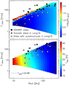 |
Fig. 9 Distribution of the underestimation factor and dust temperature in the parameter space of {F1.3 mm, Rout}. Upper panel: Λ1.3 mm asafunction of F1.3 mm and Rout. Black dots stand for the DSHARP disks. The black star represents the DoAr 33 disk. Smooth disks and disks with substructures observed in Long et al. (2019) are indicated with gray dots and gray rings, respectively. All the flux densities are scaled to the distance of 140 pc. Bottom panel: Tdust as a function of F1.3 mm and Rout. The dashed line draws the contour level of 24.8 K, which is the analytic temperature simply given by 25 (L⋆/L⊙)0.25 K. |
5 Summary
The dust mass in protoplanetary disks is an important parameter characterizing the potential for planet formation. Literature studies usually derive dust masses using an analytic approach based on the optically thin assumption. Statistic analysis of dust masses obtained in this way reveals that only a few disks are able to form our Solar System or its analogs. However, protoplanetary disks, particularly in the inner regions, are probably optically thick, which might lead to a substantial underestimation on the true dust mass.
Using self-consistent radiative transfer models, we conducted a detailed parameter study to investigate to which degree dust masses can be underestimated, and how the underestimation is influenced by disk and dust properties. Our results show that mass underestimations can be a few times up to several hundreds, depending on the optical depth along the line of sight. The most significant impacts on the underestimation are produced by the outer radius of the disk, by its inclination, and by the true dust mass. We also compared models with different dust-settling approaches that control the millimeter dust scale height. The results show that the underestimation is not significantly affected, but the well-mixed model produces the strongest millimeter emission, and consequently, it needs the lowest Mdust to fit the data. Different dust-scattering modes were also tested, but the differences in the millimeter flux, dust temperature, and therefore the underestimation are generally small. Because of the prevalence of disk substructures revealed by ALMA, we also included these small-scale features in the models. The results show that their impacts on the mass underestimation is weaker than that induced by the outer radius and true dust mass of the disk.
As an application, we also conducted a detailed SED modeling for DoAr 33, which is one of the 20 disks observed by the DSHARP project. In the modeling procedure, we fixed the outer radius and inclination of the disk to the constraints set by the ALMA observations. The most probable dust masses are 7.3 and 2.3 times higher than the analytic dust mass when the DSHARP and DIANA dust opacities are adopted in the radiative transfer simulation, respectively.
A homogeneous radiative transfer modeling is a more appropriate way to determine the disk dust mass and investigate its dependence on the host stellar properties. In addition, in the analysis, multiwavelength spatially resolved data are required for better reliability.
Acknowledgements
We thank the anonymous referee for the constructive comments that highly improved the manuscript. Y.L. acknowledges the financial support by the National Natural Science Foundation of China (Grant No. 11973090), and the science research grants from the China Manned Space Project with No. CMS-CSST-2021-B06. T.H. acknowledges support from the European Research Council under the Horizon 2020 Framework Program via the ERC Advanced Grant Origins 832428. M.F. acknowledges funding from the European Research Council (ERC) under the European Union's Horizon 2020 research and innovation program (grant agreement No. 757957). G.R. acknowledges support from the Netherlands Organisation for Scientific Research (NWO, program number 016.Veni.192.233) and from an STFC Ernest Rutherford Fellowship (grant number ST/T003855/1). H.W. acknowledges the support by NSFC grant 11973091. This publication makes use of data products from the Wide-field Infrared Survey Explorer, which is a joint project of the University of California, Los Angeles, and the Jet Propulsion Laboratory/California Institute of Technology, funded by the National Aeronautics and Space Administration. PACS has been developed by a consortium of institutes led by MPE (Germany) and including UVIE (Austria); KU Leuven, CSL, IMEC (Belgium); CEA, LAM (France); MPIA (Germany); INAF-IFSI/OAA/OAP/OAT, LENS, SISSA (Italy); IAC (Spain). This development has been supported by the funding agencies BMVIT (Austria), ESA-PRODEX (Belgium), CEA/CNES (France), DLR (Germany), ASI/INAF (Italy), and CICYT/MCYT (Spain). SPIRE has been developed by a consortium of institutes led by Cardiff University (UK) and including Univ. Lethbridge (Canada); NAOC (China); CEA, LAM (France); IFSI, Univ. Padua (Italy); IAC (Spain); Stockholm Observatory (Sweden); Imperial College London, RAL, UCL-MSSL, UKATC, Univ. Sussex (UK); and Caltech, JPL, NHSC, Univ. Colorado (USA). This development has been supported by national funding agencies: CSA (Canada); NAOC (China); CEA, CNES, CNRS (France); ASI (Italy); MCINN (Spain); SNSB (Sweden); STFC, UKSA (UK); and NASA (USA). ALMA is a partnership of ESO (representing its member states), NSF (USA), and NINS (Japan), together with NRC (Canada), MOST and ASIAA (Taiwan), and KASI (Republic of Korea), in cooperation with the Republic of Chile. The Joint ALMA Observatory is operated by ESO, AUI/NRAO, and NAOJ.
Appendix A Underestimation factors for face-on and edge-on disks
In this section, we explore how the underestimation factor changes with different model parameters for face-on (i = 0°) and edge-on (i = 90°) disks. The results are shown in Fig. A.1 and A.2.
The degree of underestimation, and its variation with different mode parameters, is broadly comparable between the face-on and fiducial inclined (i = 41.8°) disks. However, the dependences of Λ on most of the explored parameters are found to be tighter for edge-on disks. For instance, when the disk is viewed face on, Λ decreases with increasing outer disk radius Rout, and it becomes insensitive to Rout when Rout ≳ 100 AU. However, for edge-on disks, a strong correlation between Λ and Rout exists for a wide range of Rout, that is, 10 ≤ Rout ≤ 100 AU. Moreover, different dust scale heights ( or H100(1 mm dust)) generally result in a similar underestimation for disks with low inclinations. Edge-on disks show clear dependences between Λ and both parameters, however.
Appendix B CSO/SHARC II observations
Through the Chinese Telescope Plan, DoAr 33 was observed with the SHARCII bolometer array (Dowell et al. 2003) on the 10.4 m Caltech Submillimeter Observatory (CSO) on Mauna Kea. SHARCII contains a 12 × 32 array of pop-up bolometers with a > 90% filling factor over the field. The field of view of the SHARCII maps was ~2′ × 0.6′, and the beam size at 350 µm is about 8.5″.
The data at 350 µm were acquired on June 5, 2015. The conditions during the observations were excellent with τ225GHz = 0.03. The observing sequence consists of a series of target scans bracketed by scans of Pollas and cal_1629m2422, serving as both absolute flux calibration and pointing calibration measurements. We used the sweep mode for the observations, in which the telescope moves in a Lissajous pattern that keeps the central regions of the maps fully sampled. The typical individual target scan time was 300 s, and 120 s was sufficient for the calibrators. We obtained a total of 15 scans on the science target. The data analysis consists of reduction of raw data with the CRUSH pipeline (Kovács 2008), flux calibration, and aperture photometry. Figure B.1 shows the reduced image. The flux density of DoAr 33 is measured to be 0.212 Jy. The total uncertainty on the flux ranges from ~ 10–20% mainly due to the uncertainties in the calibrator’s flux.
 |
Fig. B.1 CSO/SHARC II image of DoAr 33. |
Appendix C Revisiting the Herschel data
DoAr 33 was observed with Herschel within the framework of a large survey of circumstellar disks in the Ophiuchus cloud (André et al. 2010). We re-reduced the data and performed the photometry based on point-spread function (PSF) fitting, although literature aperture photometry has been reported for PACS and SPIRE data (Rebollido et al. 2015). We worked on the same observations as Rebollido et al. (2015). The PACS 70 µm and 160 µm data are from program OT1_pabraham_3, and the SPIRE data at 250, 350, and 500 µm are from the program KPGT_pandre_1. In addition, we newly report PACS 100 µm photometry, also from the KPGT_pandre_1 program. We downloaded Level2.5 data (scan and cross-scan combined) from the Herschel Science Archive (HSA), based on the recent bulk reprocessing, which had employed the pipeline versions SPG 14.2.0 for the PACS data and SPG v14.2.1 for the SPIRE data. This iteration of the data reduction includes improved versions of the pointing products, which can refine the sharpness of the PSFs especially at short wavelengths (70 and 100 µm). The maps for PACS are JSCANAM maps (Graciá-Carpio et al. 2015), which are an implementation of the SCANAMORPHOS suite of algorithms devised by Roussel (2013). These standard maps have been constructed using the pixfrac=0.1 setting for the DRIZZLE algorithm (see Fruchter & Hook 2002). For the SPIRE data, we used the maps from the standard mapper, with the point-source calibration intact (map units Jy/beam).
Observational details of Herschel data and derived photometry
For PSF references, we used the data released by the PACS and SPIRE instrument teams, that is, maps of asteroid Vesta2 and of Neptune3, respectively. For the PACS PSFs, appropriate files were available for the pixfrac, scan instrument angle, and scan speed values of the science data. We just had to regrid the fine PSF data to the somewhat coarser pixel scale of the science maps. The SPIRE PSFs were available in a pixel scale adapted to the science data. These reference PSFs were obtained using the standard scan speed for SPIRE (30″/s, sampling 18.2 Hz), while the science data were taken with the fast scan speed of the SPIRE/PACS parallel mode (60″/s, sampling 10 Hz). Potential differences in the PSF shape would remain a second-order effect (see Griffin et al. 2010, and especially the Parallel-Mode Observers' Manual4, Sect. 2.1). All reference PSFs were rotated in order to match the PSF orientation in the individual science maps, in dependence on the satellite position angles, taken from the science map fits headers.
The actual PSF photometry was performed by employing the STA RFINDER package (Diolaiti et al. 2000), which has proven to successfully cope with the circumstances in PACS maps with extended emission (e.g., Ragan et al. 2012). For SPIRE, several photometry algorithms are implemented in the Herschel data reduction environment HIPE, but their performance has mainly been tested on clean stellar or extragalactic fields (Pearson et al. 2014). For our circumstances, that is, for a point source embedded in rivalling extended emission especially at the longest Herschel wavelengths, we also employed the STARFINDER PSF photometry for the SPIRE maps. DoAr 33 was detected with high confidence in all six bands (see also the high correlation coefficients mentioned in Table C.1). During the photometry setup, we explicitly truncated the PSF maps radially. For PACS, we worked on Jy/pixel maps and were interested in the pixel-integrated flux densities. Therefore, we applied an appropriate aperture correction as tabulated in the encircled-energy-fraction files that are attached to the aforementioned PSF release (see also Balog et al. 2014). For the SPIRE maps (in Jy/beam), we were interested in the peak fluxes of the fitted PSFs when the extended background is eventually removed. STARFINDER produces these maps as a side product that just contains the appropriately scaled copies of the PSFs, depending on the brightness of the identified sources in the field. We took these maps and fit a 2D Gaussian to the source representing DoAr 33 (without extended background emission) in order to better recover the true peak flux, partly mitigating the relatively coarse pixel resolution of the SPIRE data. For a true point source, the value of the peak flux (in Jy/beam) is identical to the integrated flux of the source.
Finally, a color correction had to be applied. The PACS and SPIRE instrument teams provide correction factors for different types of SEDs, in particular, for the situation of modified black-body SEDs (Fv ~ B(T)· vβ) We therefore fit the 70–500 µm SED with a simple but robust SED-fitting tool (Beuther & Steinacker 2007). The SED of DoAr 33 in the far-IR cannot be approximated with one temperature component, but the inclusion of two temperature components (fit values: 12.6 K and 32.5 K) gave satisfactory results when we adopted β = +2 (a case that is explicitly listed in the color-correction tables). For all six Herschel wavelengths, the tool gave the relative flux contributions for the two temperature components. We applied the color-correction terms (interpolated to the temperatures described above) to the respective fractions of the measured flux values, and summed the two corrected values per wavelength. The finally derived flux densities for DoAr 33 are given in Table C.1. The formal fitting errors from the PSF photometry are quite small. We therefore quote the sum of instrument calibration uncertainties and a second term arising from uncertainties in the underlying models of the flux calibration standards as overall uncertainties. These uncertainties are (2.0 + 5.0)% for PACS and (1.5 + 4.0)% for SPIRE, respectively.
On the whole, we can confirm the PACS 70 µm and 160 µm photometry derived by Rebollido et al. (2015, see our Table C.1). However, we derived SPIRE fluxes that are three to four times higher than reported by their study. It remains speculation to assume that the photometry for the incorrect SPIRE source was given in the paper (and in the associated Vizier catalog). Therefore, we have to conclude that their automatized aperture photometry did not handle the subtraction of the extended background well in this case, and this led to a strong oversubtraction of flux.
References
- ALMA Partnership (Brogan, C. L., et al.) 2015, ApJ, 808, L3 [Google Scholar]
- André, P., Men’shchikov, A., Bontemps, S., et al. 2010, A&A, 518, A102 [Google Scholar]
- Andrews, S. M. 2020, ARA&A, 58, 483 [Google Scholar]
- Andrews, S. M., & Williams, J. P. 2007, ApJ, 671, 1800 [CrossRef] [Google Scholar]
- Andrews, S. M., Wilner, D. J., Hughes, A. M., Qi, C., & Dullemond, C. P. 2010, ApJ, 23, 1241 [NASA ADS] [CrossRef] [Google Scholar]
- Andrews, S. M., Rosenfeld, K. A., Kraus, A. L., & Wilner, D. J. 2013, ApJ, 771, 129 [Google Scholar]
- Andrews, S. M., Huang, J., Pérez, L. M., et al. 2018a, ApJ, 869, L41 [NASA ADS] [CrossRef] [Google Scholar]
- Andrews, S. M., Terrell, M., Tripathi, A., et al. 2018b, ApJ, 865, 157 [Google Scholar]
- Ansdell, M., Williams, J. P., van der Marel, N., et al. 2016, ApJ, 828, 46 [Google Scholar]
- Ansdell, M., Williams, J. P., Trapman, L., et al. 2018, ApJ, 859, 21 [NASA ADS] [CrossRef] [Google Scholar]
- Avenhaus, H., Quanz, S. P., Garufi, A., et al. 2018, ApJ, 863, 44 [NASA ADS] [CrossRef] [Google Scholar]
- Ballering, N. P., & Eisner, J. A. 2019, AJ, 157, 144 [Google Scholar]
- Balog, Z., Rieke, G. H., Muzerolle, J., et al. 2008, ApJ, 688, 408 [NASA ADS] [CrossRef] [Google Scholar]
- Balog, Z., Müller, T., Nielbock, M., et al. 2014, Exp. Astron., 37, 129 [Google Scholar]
- Barenfeld, S. A., Carpenter, J. M., Ricci, L., & Isella, A. 2016, ApJ, 827, 142 [Google Scholar]
- Beckwith, S. V. W., Sargent, A. I., Chini, R. S., & Guesten, R. 1990, AJ, 99, 924 [Google Scholar]
- Bergin, E. A., & Williams, J. P. 2017, in Astrophys. Space Sci. Lib., 445, 1 [NASA ADS] [CrossRef] [Google Scholar]
- Bergin, E. A., Cleeves, L. I., Gorti, U., et al. 2013, Nature, 493, 644 [Google Scholar]
- Beuther, H., & Steinacker, J. 2007, ApJ, 656, L85 [NASA ADS] [CrossRef] [Google Scholar]
- Birnstiel, T., Fang, M., & Johansen, A. 2016, Space Sci. Rev., 205, 41 [Google Scholar]
- Birnstiel, T., Dullemond, C. P., Zhu, Z., et al. 2018, ApJ, 869, L45 [CrossRef] [Google Scholar]
- Bruggeman, D. 1935, Ann. Phys., 416, 416 [Google Scholar]
- Carrasco-González, C., Sierra, A., Flock, M., et al. 2019, ApJ, 883, 71 [Google Scholar]
- Cazzoletti, P., van Dishoeck, E. F., Pinilla, P., et al. 2018, A&A, 619, A161 [NASA ADS] [CrossRef] [EDP Sciences] [Google Scholar]
- Cazzoletti, P., Manara, C. F., Liu, H. B., et al. 2019, A&A, 626, A11 [NASA ADS] [CrossRef] [EDP Sciences] [Google Scholar]
- Cieza, L. A., Ruíz-Rodríguez, D., Hales, A., et al. 2019, MNRAS, 482, 698 [Google Scholar]
- Cieza, L. A., González-Ruilova, C., Hales, A. S., et al. 2021, MNRAS, 501, 2934 [Google Scholar]
- Cox, E. G., Harris, R. J., Looney, L. W., et al. 2017, ApJ, 851, 83 [Google Scholar]
- Cutri, R. M., et al. 2013, VizieR Online Data Catalog: 2328 [Google Scholar]
- Daemgen, S., Natta, A., Scholz, A., et al. 2016, A&A, 594, A83 [NASA ADS] [CrossRef] [EDP Sciences] [Google Scholar]
- Diolaiti, E., Bendinelli, O., Bonaccini, D., et al. 2000, A&As, 147, 335 [NASA ADS] [CrossRef] [EDP Sciences] [Google Scholar]
- Dong, R., Liu, S.-Y., Eisner, J., et al. 2018, ApJ, 860, 124 [NASA ADS] [CrossRef] [Google Scholar]
- Dorschner, J., Begemann, B., Henning, T., Jaeger, C., & Mutschke, H. 1995, A&A, 300, 503 [Google Scholar]
- Dowell, C. D., Allen, C. A., Babu, R. S., et al. 2003, in Proc. SPIE, 4855, 73 [Google Scholar]
- Drazkowska, J., Bitsch, B., Lambrechts, M., et al. 2022, ArXiv e-prints [arXiv:2203.09759] [Google Scholar]
- Dubrulle, B., Morfill, G., & Sterzik, M. 1995, Icarus, 114, 237 [Google Scholar]
- Dullemond, C. P., & Dominik, C. 2004, A&A, 421, 1075 [NASA ADS] [CrossRef] [EDP Sciences] [Google Scholar]
- Dullemond, C. P., Juhasz, A., Pohl, A., et al. 2012, RADMC-3D: A multipurpose radiative transfer tool, Astrophysics Source Code Library [record ascl:1202.015] [Google Scholar]
- Dullemond, C. P., Birnstiel, T., Huang, J., et al. 2018, ApJ, 869, L46 [NASA ADS] [CrossRef] [Google Scholar]
- Ercolano, B., & Pascucci, I. 2017, Roy. Soc. Open Sci., 4, 170114 [Google Scholar]
- Fedele, D., Tazzari, M., Booth, R., et al. 2018, A&A, 610, A24 [NASA ADS] [CrossRef] [EDP Sciences] [Google Scholar]
- Flaherty, K. M., Hughes, A. M., Rose, S. C., et al. 2017, ApJ, 843, 150 [NASA ADS] [CrossRef] [Google Scholar]
- Flaherty, K. M., Hughes, A. M., Simon, J. B., et al. 2020, ApJ, 895, 109 [NASA ADS] [CrossRef] [Google Scholar]
- Fruchter, A. S., & Hook, R. N. 2002, PASP, 114, 144 [NASA ADS] [CrossRef] [Google Scholar]
- Gaia Collaboration (Brown, A. G. A., et al.) 2018, A&A, 616, A1 [NASA ADS] [CrossRef] [EDP Sciences] [Google Scholar]
- Garcia, A. J. L., & Gonzalez, J.-F. 2020, MNRAS, 493, 1788 [Google Scholar]
- Graciá-Carpio, J., Wetzstein, M., & Roussel, H. 2015, ASP Conf. Ser., 512, 379 [Google Scholar]
- Gräfe, C., Wolf, S., Guilloteau, S., et al. 2013, A&A, 553, A69 [NASA ADS] [CrossRef] [EDP Sciences] [Google Scholar]
- Grant, S. L., Espaillat, C. C., Wendeborn, J., et al. 2021, ApJ, 913, 123 [NASA ADS] [CrossRef] [Google Scholar]
- Griffin, M. J., Abergel, A., Abreu, A., et al. 2010, A&A, 518, A3 [Google Scholar]
- Guidi, G., Isella, A., Testi, L., et al. 2022, A&A, 664, A137 [NASA ADS] [CrossRef] [EDP Sciences] [Google Scholar]
- Hendler, N. P., Mulders, G. D., Pascucci, I., et al. 2017, ApJ, 841, 116 [Google Scholar]
- Herczeg, G. J., & Hillenbrand, L. A. 2014, ApJ, 786, 97 [Google Scholar]
- Huang, J., Andrews, S. M., Dullemond, C. P., et al. 2018, ApJ, 869, L42 [NASA ADS] [CrossRef] [Google Scholar]
- Juhász, A., Bouwman, J., Henning, T., et al. 2010, ApJ, 721, 431 [Google Scholar]
- Kley, W., & Nelson, R. P. 2012, ARA&A, 50, 211 [Google Scholar]
- Kovács, A. 2008, in Proc. SPIE, 7020, Millimeter and Submillimeter Detectors and Instrumentation for Astronomy IV, 70201S [Google Scholar]
- Kurucz, R. 1994, Solar Abundance Model Atmospheres for 0,1,2,4,8 km/s. Kurucz CD-ROM No. 19 (Cambridge, MA: Smithsonian Astrophysical Observatory), 19 [Google Scholar]
- Law, C. J., Teague, R., Loomis, R. A., et al. 2021, ApJS, 257, 4 [NASA ADS] [CrossRef] [Google Scholar]
- Liu, H. B. 2019, ApJ, 877, L22 [NASA ADS] [CrossRef] [Google Scholar]
- Liu, Y., Henning, T., Carrasco-González, C., et al. 2017, A&A, 607, A74 [NASA ADS] [CrossRef] [EDP Sciences] [Google Scholar]
- Liu, Y., Dipierro, G., Ragusa, E., et al. 2019, A&A, 622, A75 [NASA ADS] [CrossRef] [EDP Sciences] [Google Scholar]
- Liu, Y., Bertrang, G. H. M., Flock, M., et al. 2022, Science China Physics, Mechanics & Astronomy, 65, 12, 129511 [CrossRef] [Google Scholar]
- Long, F., Pinilla, P., Herczeg, G. J., et al. 2018, ApJ, 869, 17 [Google Scholar]
- Long, F., Herczeg, G. J., Harsono, D., et al. 2019, ApJ, 882, 49 [Google Scholar]
- Long, F., Andrews, S. M., Rosotti, G., et al. 2022, ApJ, 931, 6 [NASA ADS] [CrossRef] [Google Scholar]
- Machida, M. N., Kokubo, E., Inutsuka, S.-I., & Matsumoto, T. 2010, MNRAS, 405, 1227 [Google Scholar]
- Macías, E., Espaillat, C. C., Ribas, Á., et al. 2018, ApJ, 865, 37 [Google Scholar]
- Macías, E., Guerra-Alvarado, O., Carrasco-González, C., et al. 2021, A&A, 648, A33 [EDP Sciences] [Google Scholar]
- Manara, C. F., Morbidelli, A., & Guillot, T. 2018, A&A, 618, L3 [NASA ADS] [CrossRef] [EDP Sciences] [Google Scholar]
- Maucó, K., Briceño, C., Calvet, N., et al. 2018, ApJ, 859, 1 [CrossRef] [Google Scholar]
- McClure, M. K., Bergin, E. A., Cleeves, L. I., et al. 2016, ApJ, 831, 167 [Google Scholar]
- Menu, J., van Boekel, R., Henning, T., et al. 2014, A&A, 564, A93 [NASA ADS] [CrossRef] [EDP Sciences] [Google Scholar]
- Min, M., Hovenier, J. W., & de Koter, A. 2005, A&A, 432, 909 [NASA ADS] [CrossRef] [EDP Sciences] [Google Scholar]
- Miotello, A., Bruderer, S., & van Dishoeck, E. F. 2014, A&A, 572, A96 [NASA ADS] [CrossRef] [EDP Sciences] [Google Scholar]
- Miotello, A., van Dishoeck, E. F., Kama, M., & Bruderer, S. 2016, A&A, 594, A85 [NASA ADS] [CrossRef] [EDP Sciences] [Google Scholar]
- Miotello, A., Kamp, I., Birnstiel, T., Cleeves, L. I., & Kataoka, A. 2022, Proceedings of the 34th International Cosmic Ray Conference (ICRC2015), 30 July - 6 August, 2015, The Hague, The Netherlands [Google Scholar]
- Mordasini, C., Alibert, Y., Klahr, H., & Henning, T. 2012, A&A, 547, A111 [NASA ADS] [CrossRef] [EDP Sciences] [Google Scholar]
- Mulders, G. D., Pascucci, I., Ciesla, F. J., & Fernandes, R. B. 2021, ApJ, 920, 66 [NASA ADS] [CrossRef] [Google Scholar]
- Najita, J. R., & Kenyon, S. J. 2014, MNRAS, 445, 3315 [NASA ADS] [CrossRef] [Google Scholar]
- Ohashi, S., & Kataoka, A. 2019, ApJ, 886, 103 [Google Scholar]
- Ormel, C. W., Spaans, M., & Tielens, A. G. G. M. 2007, A&A, 461, 215 [NASA ADS] [CrossRef] [EDP Sciences] [Google Scholar]
- Pascucci, I., Testi, L., Herczeg, G. J., et al. 2016, ApJ, 831, 125 [Google Scholar]
- Pascucci, I., Cabrit, S., Edwards, S., et al. 2022, ArXiv e-prints [arXiv:2203.10068] [Google Scholar]
- Pearson, C., Lim, T., North, C., et al. 2014, Exp. Astron., 37, 175 [NASA ADS] [CrossRef] [Google Scholar]
- Pérez, L. M., Benisty, M., Andrews, S. M., et al. 2018, ApJ, 869, L50 [CrossRef] [Google Scholar]
- Pinilla, P., Quiroga-Nuñez, L. H., Benisty, M., et al. 2017, ApJ, 846, 70 [Google Scholar]
- Picogna, G., Ercolano, B., Owen, J. E., & Weber, M. L. 2019, MNRAS, 487, 691 [Google Scholar]
- Pinte, C., Padgett, D. L., Ménard, F., et al. 2008, A&A, 489, 633 [NASA ADS] [CrossRef] [EDP Sciences] [Google Scholar]
- Pinte, C., Dent, W. R. F., Ménard, F., et al. 2016, ApJ, 816, 25 [Google Scholar]
- Powell, D., Gao, P., Murray-Clay, R., & Zhang, X. 2022, Nat. Astron., 6, 1147 [CrossRef] [Google Scholar]
- Ragan, S., Henning, T., Krause, O., et al. 2012, A&A, 547, A49 [NASA ADS] [CrossRef] [EDP Sciences] [Google Scholar]
- Rebollido, I., Merín, B., Ribas, Á., et al. 2015, A&A, 581, A30 [NASA ADS] [CrossRef] [EDP Sciences] [Google Scholar]
- Ribas, Á., Espaillat, C. C., Macías, E., & Sarro, L. M. 2020, A&A, 642, A171 [NASA ADS] [CrossRef] [EDP Sciences] [Google Scholar]
- Ricci, L., Testi, L., Natta, A., et al. 2010, A&A, 512, A15 [CrossRef] [EDP Sciences] [Google Scholar]
- Ricci, L., Isella, A., Carpenter, J. M., & Testi, L. 2013, ApJ, 764, L27 [NASA ADS] [CrossRef] [Google Scholar]
- Ricci, L., Testi, L., Natta, A., et al. 2014, ApJ, 791, 20 [CrossRef] [Google Scholar]
- Rich, E. A., Teague, R., Monnier, J. D., et al. 2021, ApJ, 913, 138 [NASA ADS] [CrossRef] [Google Scholar]
- Rilinger, A. M., & Espaillat, C. C. 2021, ApJ, 921, 182 [NASA ADS] [CrossRef] [Google Scholar]
- Roussel, H. 2013, PASP, 125, 1126 [Google Scholar]
- Schräpler, R., & Henning, T. 2004, ApJ, 614, 960 [CrossRef] [Google Scholar]
- Segura-Cox, D. M., Schmiedeke, A., Pineda, J. E., et al. 2020, Nature, 586, 228 [NASA ADS] [CrossRef] [Google Scholar]
- Sheehan, P. D., Tobin, J. J., Federman, S., Megeath, S. T., & Looney, L.W. 2020, ApJ, 902, 141 [NASA ADS] [CrossRef] [Google Scholar]
- Sierra, A., & Lizano, S. 2020, ApJ, 892, 136 [Google Scholar]
- Sierra, A., Pérez, L. M., Zhang, K., et al. 2021, ApJS, 257, 14 [NASA ADS] [CrossRef] [Google Scholar]
- Teague, R., Henning, T., Guilloteau, S., et al. 2018, ApJ, 864, 133 [NASA ADS] [CrossRef] [Google Scholar]
- Testi, L., Birnstiel, T., Ricci, L., et al. 2014, in Protostars and Planets VI, eds. H. Beuther, R. S. Klessen, C. P. Dullemond, & T. Henning, 339 [Google Scholar]
- Testi, L., Natta, A., Scholz, A., et al. 2016, A&A, 593, A111 [NASA ADS] [CrossRef] [EDP Sciences] [Google Scholar]
- Toci, C., Rosotti, G., Lodato, G., Testi, L., & Trapman, L. 2021, MNRAS, 507, 818 [NASA ADS] [CrossRef] [Google Scholar]
- Toon, O. B., & Ackerman, T. P. 1981, Appl. Opt., 20, 3657 [Google Scholar]
- Trapman, L., Facchini, S., Hogerheijde, M. R., van Dishoeck, E. F., & Bruderer, S. 2019, A&A, 629, A79 [NASA ADS] [CrossRef] [EDP Sciences] [Google Scholar]
- Tychoniec, Ł., Manara, C. F., Rosotti, G. P., et al. 2020, A&A, 640, A19 [NASA ADS] [CrossRef] [EDP Sciences] [Google Scholar]
- Ueda, T., Kataoka, A., & Tsukagoshi, T. 2020, ApJ, 893, 125 [Google Scholar]
- van Boekel, R., Henning, T., Menu, J., et al. 2017, ApJ, 837, 132 [Google Scholar]
- van der Marel, N., van Dishoeck, E. F., Bruderer, S., et al. 2013, Science, 340, 1199 [Google Scholar]
- van der Plas, G., Ménard, F., Ward-Duong, K., et al. 2016, ApJ, 819, 102 [NASA ADS] [CrossRef] [Google Scholar]
- Villenave, M., Ménard, F., Dent, W. R. F., et al. 2020, A&A, 642, A164 [EDP Sciences] [Google Scholar]
- Wilking, B. A., Meyer, M. R., Robinson, J. G., & Greene, T. P. 2005, AJ, 130, 1733 [NASA ADS] [CrossRef] [Google Scholar]
- Williams, J. P., & Best, W. M. J. 2014, ApJ, 788, 59 [Google Scholar]
- Williams, J. P., & Cieza, L. A. 2011, ARA&A, 49, 67 [Google Scholar]
- Woitke, P., Min, M., Pinte, C., et al. 2016, A&A, 586, A103 [NASA ADS] [CrossRef] [EDP Sciences] [Google Scholar]
- Wolf, S., Schegerer, A., Beuther, H., Padgett, D. L., & Stapelfeldt, K. R. 2008, ApJ, 674, L101 [NASA ADS] [CrossRef] [Google Scholar]
- Zhu, Z., Zhang, S., Jiang, Y.-F., et al. 2019, ApJ, 877, L18 [NASA ADS] [CrossRef] [Google Scholar]
- Zubko, V. G., Mennella, V., Colangeli, L., & Bussoletti, E. 1996, MNRAS, 282, 1321 [Google Scholar]
All Tables
All Figures
|
Fig. 1 Vertical density profile of the fiducial model at a radius of R = 10 AU. The model includes 32 grains sizes logarithmically spaced from amin = 0.01 µm to amax = 1 mm. The results are shown here for dust grains with three representative sizes, i.e., 0.01 µm (dotted line), 10 µm (dashed line), and 1 mm (solid line). |
| In the text | |
|
Fig. 2 Mass absorption coefficient κν at λ = 1.3 mm as a function of grain size a. The blue line shows the result by using the DSHARP dust model, and the case for the DIANA dust model is indicated with the black line. The horizontal dashed line marks the value of 2.3 cm2 g−1 that is commonly adopted to derive the analytic dust mass Mdust.ana in the literature. |
| In the text | |
|
Fig. 3 Properties of the fiducial model with parameters given in Table 1. Upper panel: 2D dust density distribution. The blue and black lines draw the contour of τ1.3 mm = 1 when the disk is viewed at i = 41.8°, and the lines include the DSHARP and DIANA dust opacities, respectively. Bottom panel: model SEDs when the DSHARP (blue line) or DIANA (black line) opacities are adopted in the simulation. The dashed curve stands for the input photospheric spectrum with Teff = 4000 K, assuming log g = 3.5 and solar metallicity (Kurucz 1994). |
| In the text | |
|
Fig. 4 Effects of model parameters on the results. Top row: flux densities at 0.88 and 1.3 mm (F0.88 mm and F1.3 mm, on the left Y-axis) and mass-averaged dust temperature (Tdust, on the right Y-axis) as a function of different model parameters. Bottom row: underestimation factor (Λ0.88 mm and Λ1.3 mm) as a function of different model parameters. When one particular parameter was explored, all the remaining parameters were fixed to their fiducial values listed in Table 1. The red dashed lines show the underestimation factors Λ1.3 mm that were calculated by assuming a constant Tdust = 25 (L⋆/L⊙)0.25 = 24.5 K and κ1.3 mm = 2.3 cm2 g−1. |
| In the text | |
|
Fig. 5 Scale height of 1 mm dust as a function of R. The blue line shows the fiducial model with the dust settling prescribed by Eq. (5). The black and red lines stand for models when dust settling is parameterized according to Eq. (10) under different turbulence strengths αturb. |
| In the text | |
|
Fig. 6 Comparison of Λ1.3 mm (squares) and Tdust (filled circles) between models that use the DSHARP (blue symbols) and DIANA (black symbols) dust opacities in the simulation, respectively. Details can be found in Sect. 3.4. |
| In the text | |
|
Fig. 7 Effects of disk substructures on the mass underestimation. Left column: representative 1.3 mm dust continuum image for each scenario of disk substructures. The raw radiative transfer images are convolved with a Gaussian beam of 35 mas in size (~ 5 AU at the distance of 140 pc, indicated with the filled white circle in the lower left corner of each image). The disk is seen face-on merely for a better presentation of the disk configuration. Middle column: 1.3 mm flux density (F1.3 mm) and mass-averaged temperature (Tdust) as a function of total dust mass (Mdust). When we simulated the SED, the fiducial inclination of 41.8° was adopted. Right column: underestimation factor as a function of Mdust. The green filled circles refer to the underestimation factors for smooth disks that have an equivalent Rout to that of the disks with substructures; see Sect. 3.5. |
| In the text | |
|
Fig. 8 Fitting results of the DoAr 33 disk. Panel a: SEDs of DoAr 33. The best-fit radiative transfer models using the DSHARP and DIANA opacities are shown with solid blue and black lines, respectively. The dashed line refers to the input photospheric spectrum, and observational data points are overlaid with red dots. Panels b–e: Bayesian probability distributions for Log10(Mdust/M⊙), Log10(amax/mm), |
| In the text | |
|
Fig. 9 Distribution of the underestimation factor and dust temperature in the parameter space of {F1.3 mm, Rout}. Upper panel: Λ1.3 mm asafunction of F1.3 mm and Rout. Black dots stand for the DSHARP disks. The black star represents the DoAr 33 disk. Smooth disks and disks with substructures observed in Long et al. (2019) are indicated with gray dots and gray rings, respectively. All the flux densities are scaled to the distance of 140 pc. Bottom panel: Tdust as a function of F1.3 mm and Rout. The dashed line draws the contour level of 24.8 K, which is the analytic temperature simply given by 25 (L⋆/L⊙)0.25 K. |
| In the text | |
 |
Fig. A.1 Same as in Fig. 4, but the disk inclination is fixed to i = 0° for all models. |
| In the text | |
 |
Fig. A.2 Same as in Fig. 4, but the disk inclination is fixed to i = 90° for all models. |
| In the text | |
|
Fig. B.1 CSO/SHARC II image of DoAr 33. |
| In the text | |
Current usage metrics show cumulative count of Article Views (full-text article views including HTML views, PDF and ePub downloads, according to the available data) and Abstracts Views on Vision4Press platform.
Data correspond to usage on the plateform after 2015. The current usage metrics is available 48-96 hours after online publication and is updated daily on week days.
Initial download of the metrics may take a while.