| Issue |
A&A
Volume 653, September 2021
|
|
|---|---|---|
| Article Number | A46 | |
| Number of page(s) | 14 | |
| Section | Interstellar and circumstellar matter | |
| DOI | https://doi.org/10.1051/0004-6361/202140496 | |
| Published online | 06 September 2021 | |
Probing protoplanetary disk evolution in the Chamaeleon II region
1
Univ. Grenoble Alpes, CNRS, IPAG,
38000
Grenoble,
France
2
European Southern Observatory, Alonso de Córdova 3107,
Vitacura, Casilla 19001,
Santiago 19,
Chile
3
Jet Propulsion Laboratory, California Institute of Technology,
4800 Oak Grove Drive,
Pasadena,
CA
91109,
USA
e-mail: marion.f.villenave@jpl.nasa.gov
4
Joint ALMA Observatory,
Alonso de Córdova 3107,
Vitacura
763-0355,
Santiago,
Chile
5
Unidad Mixta Internacional Franco-Chilena de Astronomía (CNRS, UMI 3386), Departamento de Astronomía, Universidad de Chile,
Camino El Observatorio 1515,
Las Condes,
Santiago,
Chile
6
Institute for Astronomy, University of Hawaii,
Honolulu,
Hawaii,
USA
7
NASA Headquarters,
300 E Street SW,
Washington,
DC
20546,
USA
8
Departamento de Ciencias Fisicas, Facultad de Ciencias Exactas,
Universidad Andres Bello. Av. Fernandez Concha 700,
Las Condes,
Santiago,
Chile
9
Núcleo Milenio de Formación Planetaria (NPF),
Av. Gran Bretaña 1111,
Valparaiso,
Chile
10
Aurora Technology for ESA/ESAC, Camino bajo del Castillo s/n, Urbanización Villafranca del Castillo, Villanueva de la Cañada,
28692
Madrid,
Spain
11
Núcleo de Astronomía, Facultad de Ingeniería y Ciencias, Universidad Diego Portales,
Av. Ejercito 441,
Santiago,
Chile
12
National Radio Astronomy Observatory,
520 Edgemont Road,
Charlottesville,
Virginia,
22903-2475,
USA
13
Kapteyn Astronomical Institute, University of Groningen,
Landleven 12,
9747
AD
Groningen,
The Netherlands
14
School of Physics and Astronomy, Monash University,
Clayton,
Vic
3800,
Australia
15
Massachusetts Institute of Technology, Kavli Institute for Astrophysics and Space Research,
Cambridge,
MA
02109,
USA
16
Universidad Técnica Federico Santa María, Departamento de Física,
Avenida España
1680,
Valparaíso,
Chile
Received:
4
February
2021
Accepted:
22
June
2021
Context. Characterizing the evolution of protoplanetary disks is necessary to improve our understanding of planet formation. Constraints on both dust and gas are needed to determine the dominant disk dissipation mechanisms.
Aims. We aim to compare the disk dust masses in the Chamaeleon II (Cha II) star-forming region with other regions with ages between 1 and 10 Myr.
Methods. We use ALMA band 6 observations (1.3 mm) to survey 29 protoplanetary disks in Cha II. Dust mass estimates are derived from the continuum data.
Results. Out of our initial sample of 29 disks, we detect 22 sources in the continuum, 10 in 12CO, 3 in 13CO, and none in C18O (J = 2−1). Additionally, we detect two companion candidates in the continuum and 12CO emission. Most disk dust masses are lower than 10 M⊕, assuming thermal emission from optically thin dust. Including non-detections, we derive a median dust mass of 4.5 ± 1.5 M⊕ from survival analysis. We compare consistent estimations of the distributions of the disk dust mass and the disk-to-stellar mass ratios in Cha II with six other low mass and isolated star-forming regions in the age range of 1–10 Myr: Upper Sco, CrA, IC 348, Cha I, Lupus, and Taurus. When comparing the dust-to-stellar mass ratio, we find that the masses of disks in Cha II are statistically different from those in Upper Sco and Taurus, and we confirm that disks in Upper Sco, the oldest region of the sample, are statistically less massive than in all other regions. Performing a second statistical test of the dust mass distributions from similar mass bins, we find no statistical differences between these regions and Cha II.
Conclusions. We interpret these trends, most simply, as a sign of decline in the disk dust masses with time or dust evolution. Different global initial conditions in star-forming regions may also play a role, but their impact on the properties of a disk population is difficult to isolate in star-forming regions lacking nearby massive stars.
Key words: protoplanetary disks / stars: formation / circumstellar matter / stars: variables: T Tauri, Herbig Ae/Be
© M. Villenave et al. 2021
 Open Access article, published by EDP Sciences, under the terms of the Creative Commons Attribution License (https://creativecommons.org/licenses/by/4.0), which permits unrestricted use, distribution, and reproduction in any medium, provided the original work is properly cited.
1 Introduction
Planets are thought to form in gas- and dust-rich protoplanetary disks that orbit young stars. Characterizing the physical properties and evolutionary mechanisms of protoplanetary disks is therefore essential for the understanding of planet formation. Various infrared studies have shown that the typical dissipation timescale of protoplanetary disks is about 3 Myr (e.g., Mamajek 2009; Ribas et al. 2014), the oldest disks typically being up to 10 Myr old. However, these observations trace either small, warm dust particles (in the continuum) or accretion signatures (Fedele et al. 2010), which are not sensitive to the dissipation of the bulk gas and dust mass, more relevant for planet formation.
More recently, the Atacama Large Millimeter/submillimeter Array (ALMA) has allowed a number of statistical surveys of the disk dust mass to be performed in various star-forming regions. Many surveys have focused on relatively young, 1–3 Myr, regions (Taurus, Chamaeleon I, Lupus, Ophiuchus, IC348, ONC, CrA, OMC-2, Lynds 1641; Andrews et al. 2013; Pascucci et al. 2016; Ansdell et al. 2016; Cieza et al. 2019; Ruíz-Rodríguez et al. 2018; Eisner et al. 2018; Cazzoletti et al. 2019; van Terwisga et al. 2019; Grant et al. 2021). They showed that the disk dust masses estimated in these young regions are in general larger than those measured in a more evolved star-forming region (5–10Myr, Upper Sco; Barenfeld et al. 2016; van der Plas et al. 2016). This result indicates that the disk dust mass decreases with time. In addition, several surveys of intermediate age star-forming regions have also been performed (σ-Orionis, λ-Orionis; Ansdell et al. 2017, 2020). However, those mostly focus on regions that include massive stars. They find that massive stars can have an important impact on the evolution of disks. Further studies of intermediately aged regions, unaffected by external factors of disk evolution, are required to study dust disk dissipation.
In this context, the Chamaeleon II (Cha II) star-forming region is of particular interest. Its age was historically estimated to be 4 ± 2 Myr (Spezzi et al. 2008), which made it a good choice for studying the evolution of gas and dust content. However, we note that a recent study revised the age of the region using Gaia Data Release 2 (DR2) distances (Galli et al. 2021). That study suggests that Cha II is significantly younger, with a median age of 1–2 Myr. This new age is consistent with the high disk fraction observed in previous infrared surveys (e.g., Ribas et al. 2014). Cha II is a close-by region, located at an average distance of 198 pc (Dzib et al. 2018; Galli et al. 2021). It has been the target of several infrared studies (Alcalá et al. 2008; Spezzi et al. 2008, 2013), which have shown that the region is quite isolated and does not contain high mass stars. Thus, the evolution of its disks is likely not driven by external factors, permitting the study of isolated disk evolution.
In this paper, we present an ALMA survey of the Class II disks of Cha II. We describe our ALMA observations and data reduction inSect. 2, and present the continuum and CO line measurements in Sect. 3. In Sect. 4, we analyze the dust properties of the Cha II disks. We estimate the dust masses and compare the dust-to-star mass ratio with different star-forming regions. Our results are summarized in Sect. 5.
2 Observations and data reduction
2.1 Sample
Our observations focus on 29 protoplanetary disks that were selected based on their infrared emission at 70 μm from Herschel observations (Spezzi et al. 2013). Specifically, we observed 18 out of the 19 Class II disks detected at 70 μm by Spezzi et al. (2013), and 9 out of the 19 non-detected Class II disks at 70 μm (see Appendix A). We also observed one Class I disk detected at 70 μm and one “flat spectrum” source that was notdetected at 70 μm. To summarize, the sample includes one Class I source, one flat spectrum source, and 27 Class II sources; two secondary sources (around Hn 24 and Sz 59) were also detected in our ALMA observations (see Sect. 3.1), leading to a total sample of 31 objects.
We checked the membership of each observed target by using distances from Gaia data releases and the recent membership analysis performed by Galli et al. (2021, their Table A.2). We find that 19 disks included in our sample were confirmed as members by Galli et al. (2021). We classify these sources as “Members” in Table 1 and we report the individual distances as estimated by Galli et al. (2021). We also identified five sources, rejected or not included in the study of Galli et al. (2021), as likely cluster members given their latest Gaia EDR3 distance (Gaia Collaboration 2021). Their Gaia EDR3 distances lieless than 20 pc away from the average cluster distance. We classify these objects as “Likely” members in Table 1, and report the individual distances calculated from the Gaia EDR3 catalog (Gaia Collaboration 2021). Two disks, namely Sz 50 and IRAS12496-7650, are located more than 40 pc away from the average cluster distance, so they are possibly foreground and background objects, respectively. For these sources, we report the distances estimated using Gaia DR2 parallaxes in Table 1, because the latest release produced less reliable results (larger parallax error for IRAS12496-7650 and no EDR3 measurement for Sz 50). Finally, three disks (J130529.0-774140, IRAS12500-7658, ISO-CHAII 13) do not have a good (or any) parallax measurement in either Gaia data releases, making them “Uncertain” cluster members.
To summarize, our sample is composed of 29 disks, including 19 Class II confirmed members of Cha II, 4 Class II likely members, and 1 flat spectrum likely member. Two Class II sources and one Class I are uncertain members, and two Class II are likely foreground and background systems, external to the Cha II star-forming region. We report the membership of each source along with its adopted distance and stellar parameters in Table 1. Additionally, 8 Class II sources, not observed in this study and observed but not detected at 70 μm (Spezzi et al. 2013) were confirmed as cluster members by Galli et al. (2021). We report these objects as “Unobserved” members in Table 1.
We note that all the Class II sources not observed in our survey but confirmed as member by Galli et al. (2021) were observed but not detected at 70 μm (Spezzi et al. 2013). In Appendix A, we show that, out of the 10 disks undetected at 70 μm included in our sample, only 3 were detected with our ALMA observations. It is thus likely that most of the unobserved Class II sources would also not have been detected with our observations.
2.2 ALMA observations
Our ALMA observations (Project 2013.1.00708.S, PI: Ménard) were obtained on 2015 August 27, with an array configuration made of 40 antennas with baselines ranging from 26 to 1170 m. The continuum spectral windows were centered on 234.2 GHz and 217.2 GHz, giving a mean continuum frequency of 225.7 GHz (1.3 mm). The other two spectral windows were set up to include three CO isotopologue lines. They covered the 12CO, 13CO, and C18O J = 2−1 transitions at 230.538 GHz, 220.399 GHz, and 219.56 GHz. Each spectral window had 0.33 km s−1 velocity resolution. The integration time was 2.5 min on-source per target giving an average continuum RMS of 0.17 mJy beam−1. We used thecalibration script provided by the observatory, with CASA (McMullin et al. 2007) version 4.3.1 to calibrate the raw data.
We produced the continuum images from the calibrated visibilities over the continuum channels by using the CASA clean function with a Briggs robust weighting parameter of + 0.5. To maximize the dynamic range of the brightest sources, we performed a phase-only self-calibration on CM Cha, Hn 22, Hn 23, IRAS12500-7658, Sz 58, and Sz 61. For these sources, we used solution intervals of the scan length (“inf”) and combined all spectral windows. In the case of the brightest target, IRAS12496-7650 (also called DK Cha), phase and amplitude self-calibration were performed. The first two iterations were phase only (solution intervals of “inf” and 6.05 s), and third round was an amplitude and phase calibration with a solution interval of the duration of the whole scan. We present the continuum images in Fig. 1. They achieve an averaged angular resolution of 0.48′′ × 0.25′′ (95 × 50 au).
We extracted 12CO, 13CO, and C18O channel maps from the calibrated visibilities after subtracting the continuum from the spectral windows containing line emission using the uvcontsub routine in CASA. For the brightest sources, we also applied the continuum self-calibration solutions to the gas line data. We cleaned the sources with velocity channels of 0.35 km s−1, and with a Briggs robust weighting parameter of 0. We obtain an average angular resolution of 0.51′′ × 0.28′′ (100 × 55 au) for the CO lines.
Using the channel maps, we generated moment 0 maps for the detected sources. We used the immoments CASA task and generated the map with all the spectral channels where the source is visually detected. In addition, we used the CO channel maps to generate line profiles for each source and isotopologue, over a range from −10 to +15 km s−1. The line profiles of each source are integrated over a unique spatial range for all channels, the size of which depends on the detectability of the corresponding isotopologue. For the sources that are detected in at least one spectral channel, theintegrating area corresponds to the ellipse that encompasses all pixels (in all channels) above a 3σ limit. We define σ as the global RMS of the channel maps where the source is not detected. On the other hand, when the sources are not detected in any channel, we used a square of size 1′′ ×1′′ (close to the mean size of the detected sources), centered near the phase center to extract the spectrum. 12CO and 13CO line profiles,and moment 0 maps of the detected sources are shown in Fig. 2.
Stellar parameters.
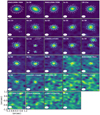 |
Fig. 1 Continuum images ordered by decreasing fluxes. Images are 2.4′′ × 2.4′′, except for Hn 24 where we use 4.8′′ × 4.8′′ to show the secondary source. The beam is shown in the lower left corner of each panel. 3σ and 15σ contours are shown in solid and dashed lines, respectively. The color map is chosen to go from −3 σ to the maximum intensity of each image. |
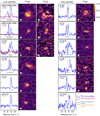 |
Fig. 2 Line profiles (left panels), 12CO normalized moment 0 maps (middle panels), and 13CO normalized moment 0 maps (right panels) for the sources detected in 12CO. Each line displays two sources. For each source, we display the continuum contours at 50% of the continuum peak (black line) and the CO contours at 50% of the CO peak (white line) on the CO moment 0 maps. The beam size is shown in the bottom left corner of each panel, along with a white line representing a 0.5′′ scale. On the line profiles plots (left panels), we also show a green vertical line at 3 km s−1, where the cloud absorption is estimated, and the size of the integration range to estimate the 12CO and 13CO fluxes reported in Table 3. The maximum fluxes of each line profile are displayed in the top left side of the panels, colored in blue for 12CO and in red for 13CO. The y ticks of the line profiles mark 0%, 50%, and 100% of the maximum fluxes. |
3 Results
3.1 Continuum emission
We measured the continuum emission by fitting an elliptical Gaussian model to the visibility data, using the CASA uvmodelfit task. This model has six free parameters: integrated flux density (F1.3mm), full width half maximum (hereafter FWHM) along the major axis (a1.3mm), aspect ratio of the axes (r), position angle (PA), and the right ascension and declination of the phase center (Δα, Δδ). If the ratio of a1.3mm to its uncertainty is less than five, we fitted the visibilities with a point source model with only three free parameters (F1.3mm, Δα, Δδ). Table 2 gives the measured 1.3 mm continuum fluxes. For the sources fitted with an elliptical Gaussian, we also report a1.3mm and PA, as well as the inclination, i, estimated from r assuming that the disks are azimuthally symmetric. For the detected sources, the phase centers from the fitting are also reported in Table 1.
Out of 31 sources, 24 are detected above a 3σ significance threshold. This includes two secondary sources, which are detected in the fields of Sz 59 and Hn 24. We measured a separation of 0.70′′ and PA of –25° for Sz 59 from the continuum fits, which is consistent with the measurement by Geoffray & Monin (2001). Hn 24 B is a new companion candidate, since it is not referenced in the literature. From the continuum fit, we measured a separation of 1.67′′ and a PA of 0°.
Additionally, our results indicate that 16 sources are also resolved in at least one direction. For six of them, even if the major axis size is well resolved by the elliptical Gaussian model, the disk was not resolved in the other direction, which implies that the inclination and position angle could not be accurately evaluated. We indicate these disks by the symbol “×” in the inclination column of Table 2. Observations at higher angular resolution are needed to estimate the inclination of these systems.
1.3 mm continuum properties.
3.2 CO line emission
We measured the line fluxes by integrating the line profile over the spectral range where the source is detected by more than 3σ. For the detected sources, the mean line width is ~ 6.3 km s−1. We represent the line width by horizontal lines at the bottom of each (left) panels of Fig. 2. For the detected sources, we estimated the flux error as the RMS of the line profile outside the source, integrated over the width of the emission. On the other hand, we report upper limits for the non-detections. They correspond to three times the RMS of the line profile, integrated over a line width of 6.3 km s−1. We present the integrated fluxes and uncertainties for the three isotopologues in Table 3.
Out of 31 targets observed, 12 are detected in 12CO, 3 in 13CO, and none in C18O. This includes the two secondary sources that are detected in 12CO only. All the sources detected in 13CO are also detected in 12CO, and all the sources detected in 12CO are detected in the continuum. Each source detected in a CO isotopologue is also spatially resolved in this isotopologue line. In the particular case of IRAS12496-7650, the 12CO and 13CO emissions appear to extend up to the maximum recoverable scale of the observations, which suggests that part of the emission is possibly filtered out. In addition, we caution the reader for the presence of significant foreground absorption for all sources. From the moment 0 maps displayed in Fig. 2, we see that the line emission of some sources is not centered on the continuum (e.g., Sz 61), which suggests that we are missing part of the emission for each of them. Furthermore, some line profiles are also asymmetric (e.g., CM Cha) and/or have minima (absorption) that go down to the continuum level (e.g., IRAS12500-7658). This is not compatible with a Keplerian profile without absorption. The large cloud absorption appears to be located around ~ 3 km s−1 (green line on Fig. 2), which is compatible with the study of Mizuno et al. (2001). There is possibly some dispersion in the cloud velocity since some sources do not show significant absorption at the reported value (e.g., Sz 63). The presence of significant cloud absorption indicates that the CO fluxes presented in Table 3 and the average line width of theprofiles can be underestimated.
Additionally, from the black and white contours in the moment maps of Fig. 2, we find that the 12CO emission is systematically larger than its continuum counterpart. This result has been observed in various other studies (e.g., van der Plas et al. 2017; Ansdell et al. 2018), and can be explained by differences in optical depth between gas and dust, or by the presence of grain growth and radial drift in the disks. However, due of the low angular resolution of our data (elongated beam) and significant foreground absorption, we could not get a reliable estimate the gas sizes. Higher angular resolution observationsand detailed modeling of each object is needed to estimate quantitatively the dust and gas sizes, and to compare the dust and gas size ratio with previous studies (e.g., Ansdell et al. 2018; Facchini et al. 2019; Trapman et al. 2019; Sanchis et al. 2021).
Integrated fluxes for the CO isotopologues derived from the line profiles.
4 Disk properties
4.1 Dust masses
Assuming that the continuum emission is optically thin at 1.3 mm, it is possible to infer the disk dust mass (Mdust) from the continuum millimetric flux (Fν) at a given wavelength (e.g., Hildebrand 1983):
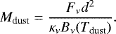 (1)
(1)
We assumed a grain opacity κν of 2.3 cm2 g−1 at 230 GHz (Beckwith et al. 1990), with κν ∝ ν0.4 (as in other studies, e.g., Andrews et al. 2013; Pascucci et al. 2016, and consistently with recent integrated spectral index measurements, e.g., Ribas et al. 2017). We used the individual Gaia distances of each object as reported in Table 1. When the sources do not have Gaia parallaxes, we used the average distance of the well characterized objects: 198 pc (Dzib et al. 2018; Galli et al. 2021). We also adopted the relationship of Tdust with L⋆ from Andrews et al. (2013), inferred with a grid of radiative transfer models: 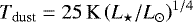 . We used the luminosities determined by Spezzi et al. (2008), rescaled to the Gaia distances. For the sources that were not characterized spectrally (Hn 24 B, J130059.3-771403, J130521.7-773810, J130529.0-774140, and Sz 59 B), we applied a characteristic dust temperature of Tdust = 20 K (Andrews & Williams 2005).
Figure 3 shows the detections and upper limits of our dust mass estimates. The values are reported in Table 2. They range from ~0.7 M⊕ (IRAS12535-7623) to ~337.5 M⊕ (IRAS12469-7650). We note, however, that the scaling relation between Tdust and L⋆ was calibrated for luminosities larger than 0.1 L⊙. In our sample, five objects have luminosities lower than this value, including IRAS12500-7658 and ISO-CHAII 13 that have luminosities close to 0.01 L⊙. For these two sources, the dust mass is probably overestimated by a factor of ~ 2 (van der Plas et al. 2017).
4.2 Comparison with other regions
Over the last years, observations of nearby star-forming regions have shown a trend for disk dust mass to decrease with age, which can be a sign for disk dissipation and/or dust evolution (e.g., Ansdell et al. 2016). In this section, we expand the study of cumulative dust mass distribution to the Cha II star-forming region, aiming to add constraints on the evolution of dust mass with time. We focus our analysis on isolated, low mass star-forming regions (see Sect. 4.2.1) for which the dissipation is likely not affected by external factors.
Previous studies have found that the dust mass (Mdust) correlates with the stellar mass (M⋆, e.g., Andrews et al. 2013; Pascucci et al. 2016; Ansdell et al. 2017; Cazzoletti et al. 2019). Because of this relation, low mass stars are expected to host less massive dust disks than more massive stars. This implies that the comparison of dust mass distributions of star-forming regions with different stellar mass distributions might lead to inadequate conclusions. In this context, some of our analysis consists in comparing the dust-to-stellar mass ratio distributions for different regions (seealso Barenfeld et al. 2016). Using this ratio allows us to reduce the impact of potentially different M⋆ distributions and, to first order, to study the evolution of Mdust as a function of time. In addition, for comparison with previous studies, we also present the dust mass distributions for the same regions.
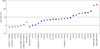 |
Fig. 3 Dust masses for the 31 sources in our Cha II sample expressed in Earth masses, ordered by increasing dust mass(Table 2). The black and red squares indicates the sources also detected in 12CO and 13CO, respectively.Round symbols show continuum only detected sources and the downward-facing triangles correspond to 3σ upper limitsfor non-detections. |
4.2.1 Sample
In this analysis, we consider seven star-forming regions observed at millimeter wavelengths and for which stellar masses can be well estimated. They are Upper Sco (Barenfeld et al. 2016), Cha II (this study), IC 348 (Ruíz-Rodríguez et al. 2018), CrA (Cazzoletti et al. 2019), Cha I (Pascucci et al. 2016), Lupus (both band 7 and band 6 surveys; Ansdell et al. 2016, 2018), and Taurus (Andrews et al. 2013). We show the main characteristics of each region (age, average distance, frequency of the observations) in Table 4. Because objects of different SED classes are most likely in a different evolutionary stage, we selected only the Class II objects from all studies. For Upper Sco, they are the objects classified as “Full,” “Transitional,” and “Evolved” in Table 1 of Barenfeld et al. (2016).
Additionally, we note that we did not include a number of other millimeter surveys in this analysis. This is either because they are located in dense or massive environments (e.g., σ-Orionis, ONC, OMC-2, NGC 2024, λ-Orionis; Ansdell et al. 2017, 2020; Eisner et al. 2018; van Terwisga et al. 2019, 2020) or because the stellar masses are not yet available (e.g., Ophiuchus, Lynds 1641; Cieza et al. 2019; Grant et al. 2021). We also did not include the SMA survey of the Serpens star-forming region (Law et al. 2017), both because less than half of the known Class II population of this region was observed and because the survey is significantly less sensitive compared to the other surveys of this study (lowest detected dust mass being ~ 12 M⊕).
4.2.2 Methods
In order to provide a meaningful comparison of all regions, we recalculated both the dust and stellar masses in a consistent and homogeneous manner.
Individual distances
We considered individual stellar distances. For Cha II, we used the distances reported in Table 1. We also excluded the sources classified as uncertain (including the two binary candidates), foreground, and background (Table 1) from this analysis. For the other star-forming regions, whenever uncertainties are smaller than 10%, we assigned thedistance of the source from the Gaia DR2 catalog (Gaia Collaboration 2018). On the other hand, for sources with larger errorsor that are not in the catalog, we used the average distance of the association (see Table 4).
Stellar masses
We determined stellar masses for all data sets in a consistent way, using isochrones from Baraffe et al. (2015) in the range 0.5–50 Myr. The tracks were interpolated to probe the mass range from 0.05 to 1.4 M⊙, by steps of 0.01 M⊙. We adopted the method described in Andrews et al. (2013) and Pascucci et al. (2016) to assign a stellar mass and an age. We first evaluated a likelihood function (Eq. (1) in Andrews et al. 2013) on each grid model, assuming that the uncertainties in log (L⋆∕L⊙) and log (T⋆∕K) are 0.1 and 0.02, respectively, which correspond to the upper values for uncertainties in Spezzi et al. (2008). We then marginalized the distribution to estimate the stellar masses and their uncertainties, corresponding to the median, 18%, and 84% percentiles, respectively (see Table 1 for Cha II).
We used stellar luminosities and temperatures from Andrews et al. (2013), Alcala et al. (2017), Manara et al. (2017), Luhman (2007), Cazzoletti et al. (2019), Ruíz-Rodríguez et al. (2018), and Barenfeld et al. (2016) for Taurus, Lupus, Cha I, CrA, IC 348, and Upper Sco, respectively. Before estimating the stellar masses, we rescaled the luminosities to each individual stellar distance.
Parameters of star-forming regions.
Dust masses
We also recalculated dust masses in a homogeneous way from millimeter or submillimetrer fluxes (from Barenfeld et al. 2016; Cazzoletti et al. 2019; Ruíz-Rodríguez et al. 2018; Pascucci et al. 2016; Ansdell et al. 2016, 2018; Andrews et al. 2013) using Eq. (1). We used the same temperature-luminosity relation and grain opacity as previously, and adopted the most recent distances. We report the mass of the least massive disk detected in each star-forming region in Table 4 (column Mdust, min).
We note that using the simplifying assumption of Tdust = 20 K does not change the statistical significance of the results presented in this section. Also, it should be noticed that our analysis includes surveys observed at different frequencies, either ALMA band 6 (~ 225 GHz) or band 7 (~340 GHz; see Table 4). Using κν ∝ ν (as in other studies, e.g., Ansdell et al. 2016; Cazzoletti et al. 2019) instead of κν ∝ ν0.4 (this study and others, e.g., Andrews et al. 2013; Pascucci et al. 2016) corresponds to a difference of less than 25% in the band 7 opacities. We checked that using either opacity law does not significantly affect the results.
Disks sub-selection
Because most of the samples used are only complete down to the brown dwarf limit, we considered only stars with derived masses above 0.1 M⊙. Moreover, as Baraffe et al. (2015) tracks stop at M⋆ = 1.4 M⊙, we decided not to include stars where the fit of isochrone produces this value. We also omitted sources for which the stellar mass is not available, even if they have a measured dust mass. We present the number of sources considered in this study along with the number of detected sources in Table 4.
4.2.3 Cumulative distributions
In order to compare all star-forming regions, we generated two families of cumulative distributions. We used the Kaplan–Meier estimator in the lifelines package in Python1, which takesinto account upper limits and was used in previous studies (e.g., Ansdell et al. 2016; Law et al. 2017). We note that the Kaplan-Meier estimator assumes that the value of a censored point is precisely known (e.g., Feigelson & Nelson 1985). While the errors on Mdust are typically of a few percent (see Table 2), the uncertainties on the ratio of Mdust/M⋆ are significantly larger (due to the larger uncertainty on M⋆; see Table 1) and have large variations between sources, which is not taken into account with this estimator.
Dust masses
First, as in previous studies, we estimated the cumulative distributions of Mdust. They are shown in the top panel of Fig. 4, and scaled so that the maximum of each distribution corresponds to the fraction of detected sources in each sample. We find that most distributions, including that of Cha II, have similar medians and shapes, but Upper Sco, CrA, and IC 348 show a noticeable difference compared with the others, with median dust masses up to one order of magnitude smaller than in other regions for Upper Sco and CrA (see penultimate column of Table 4). We note that when performing a parametric estimate of the dust mass distribution (e.g., Williams et al. 2019), we find similar results with the distributions of Upper Sco and CrA shifted to lower mass compared to the other regions. In addition to intrinsic differences in the dust mass, this might be related to different effects such as differences in stellar populations with other regions (e.g., no stars between 0.9 and 1.4 M⊙ in IC 348) or to the scaling factor used for the Mdust distribution.The later might have to be modified if further studies identify new sources in the star-forming regions studied (e.g., Galli et al. 2020a, in CrA), and if their observations at millimeter wavelength lead to a different fraction of detected sources in the samples.
Dust-to-stellar mass ratios
In order to limit the effect of different stellar populations, we also estimated cumulative distributions of dust-to-stellar mass ratio, which are shown in the bottom panel of Fig. 4. These curves go up to 1 rather than to the fraction of detected sources in each region even though disks with an upper limit on their dust mass are included. This is because of the known correlation of Mdust with M⋆. Indeed, while most non-detected systems have a lower dust mass than the detected disks (confining them to the lower mass end of the cumulative distribution of Mdust and justifying the scaling applied), most of these systems are found around low mass stars. We checked that, on average, 60% of the non-detected disks would have a Mdust∕M⋆ ratio larger than three times the lowest ratio of a detected disk in the corresponding region when using the proper upper limits (only 6% on average for Mdust). So the non-detections would be scattered all over the cumulative distribution of Mdust∕M⋆ and not only concentrated to the low end of the distribution, as it is the case for Mdust. If we were to perform more sensitive observations, these targets might be detected and have a large Mdust∕M⋆, so the distribution of this ratio should not be normalized by the fraction of detected sources as opposed to the distribution of Mdust. We note again that the Kaplan–Meier estimator takes non-detections into account.
As highlighted by the relative position of each distribution, we find that most regions appear to have similar shapes, with the exception of Taurus. The Taurus distribution has a different shape than in the plot of Mdust because a large fraction of the non-detections are around low mass stars. This leads to a large number of entries with a large Mdust/M⋆ ratio, illustrating the effect previously mentioned. It is also clear that the Upper Sco and CrA distributions have a shallower slope than the other distributions, as previously reported by Ansdell et al. (2017) and Cazzoletti et al. (2019). In the following subsection, we aim to statistically compare the different regions.
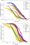 |
Fig. 4 Cumulative distributions functions generated by the Kaplan-Meier estimator. Top: cumulative distribution of the dust mass, normalized by the fraction of detected sources in each star-forming regions. Bottom: cumulative distribution of the dust-to-stellar mass ratio. The bottom distributions include disks not detected in millimeter emission. Those are scattered over the distribution of Mdust /M⋆ (see Sect. 4.2.3). We indicate 1σ confidence intervals. |
4.2.4 Statistical test
To test the statistical significance of the observed shift in the dust mass and mass ratio distributions, we performed two statistical tests on all star-forming regions. We used the logrank test, a non-parametric method that compares the survival distributions of two samples, taking into account non-detections. The null hypothesis is that distributions of all regions are equal at all mass ratios.
For the first test, we compared directly the distributions of Mdust/M⋆ ratio and present the results in Table 5. We find that Upper Sco and CrA are statistically different from all other regions except from Cha II (marginal difference between Cha II and Upper Sco), and they are statistically similar among themselves. Cha II is also statistically different from Taurus, and the other regions are statistically similar or marginally different.
We also performed a more robust statistical comparison of the dust mass distributions (Mdust), following the methodology of Andrews et al. (2013). We first divided the stellar distributions into five mass bins between 0.1 and 1.4 M⊙ and drew the same number of sources in each bin from the Cha II region (reference sample) and from other star-forming regions (comparison samples). Then, we performed a logrank test to test that the distributions are drawn from the same parent population. This process is repeated 104 times for each compared region. We present the cumulative histogram of the results in Fig. 5. As for Table 5, a low pϕ value indicates that the regions are statistically different. We find median pϕ values of 0.22, 0.40, 0.31, 0.47, 0.54, 0.08, and 0.56, respectively for Taurus, Lupus (b6), Lupus (b7), Cha I, IC 348, CrA, and Upper Sco when compared to the Cha II dust mass distribution. In other words, we find some consistency in the results with the first statistical test presented in this section: Cha II appears to be statistically similar to Lupus, Cha I, and IC 348. However, in contrast to previous results from our first test performed on Mdust/M⋆, we now find that the dust mass distribution (Mdust) of the Cha II star-forming region is also statistically similar to that of Upper Sco and Taurus, and is also potentially marginally different from CrA. The differences between the two statistical tests might indicate that the relationship of Mdust with M⋆ varies with the star-forming region considered, as found by previous studies (e.g., Ansdell et al. 2017; Cazzoletti et al. 2019). Alternatively, as previously mentioned, we note that the Kaplan–Meier and logrank tests do not take into account the uncertainties on the censored values. Those can be large in the case of Mdust with M⋆ and may lead to an overestimation of the significance of the logrank test on Mdust/M⋆. We also note that the comparison of Cha II with CrA was performed on a small number of disks (< 24 in both regions) and might not be statistically significant.
If we consider that Cha II is 4 ± 2 Myr as found by Spezzi et al. (2008), we can interpret the shift in Mdust and Mdust/M⋆ between the young regions (Taurus, Lupus, Cha I, and IC348), the intermediate Cha II, and the older regions (Upper Sco and CrA) as an evolutionary effect: the older regions being less massive (see Table 4 and Fig. 4) due either to a decline of dust mass with time or to dust evolution. When the age difference between two regions is large (e.g., ≥3 Myr), their distributions of Mdust/M⋆ are statistically different and the distributions of Mdust in similar stellar mass bins are marginally different. On the other hand, regions of similar age are statistically similar. Alternatively, a recent studyby Galli et al. (2021) suggested that the Cha II region is younger, with an age around 1–2 Myr. In that case, the shift in Mdust and Mdust/M⋆ would not be related to disk evolution but possibly to different initial conditions between the different regions (see discussions in e.g., Cazzoletti et al. 2019; Williams et al. 2019). However, the minor differences in the distributions of Mdust in similar stellar mass bins between the different regions (see Fig. 5) prevent us from drawing strong conclusions.
Results of pair comparisons with the logrank test applied on the ratio Mdust /M⋆.
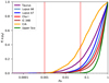 |
Fig. 5 Comparison of the dust mass distributions of different star-forming regions to that of Cha II. pϕ is the probability that the synthetic population drawn from the comparison samples and the reference sample come from the same parent population. f(≤ pϕ) is the cumulative distribution for pϕ resulting from the logrank two-sample test for censored data sets after 104 MC iterations. The vertical lines correspond to pϕ of 0.05 and 0.001, respectively. |
4.2.5 Possible limitations
To convert the observed fluxes into dust masses, we assumed that disks were optically thin at 0.9 mm and 1.3 mm, meaning that the observed continuum flux is a reliable tracer of dust mass. This assumption may be partially incorrect since substructures are found to be ubiquitous in protoplanetary disks (Andrews et al. 2018; Long et al. 2018), and often coincide with optically thick regions (e.g., Dullemond et al. 2018; Dent et al. 2019). Several studies, for example comparing the dust masses estimated from radiative transfer or physical models with those calculated with Eq. (1) (e.g., Ballering & Eisner 2019; Ribas et al. 2020), provide another indication that disks might be optically thick at 1.3 mm. Indeed, they find that the analytical masses are generally underestimated (by a factor of one to five) compared to the detailed results. Nevertheless, to facilitate the comparison with previous studies and because performing individual modeling of a large number of disks is extremely expensive, we assumed that the continuum flux is a reliable tracer of dust mass. Further surveys at longer wavelengths (e.g., Tazzari et al. 2021), expected to probe larger grains with lower millimeter opacities, will be useful to characterize with more details the decrease in dust mass with the age of the star-forming region.
Resolved and unresolved binary systems were also not filtered out from the samples. However, binary systems have been shown to disperse their disk faster than single star systems (Cieza et al. 2009; Cox et al. 2017; Zurlo et al. 2020), especially when their separation is smaller than 40 au (Kraus et al. 2012). We verified that only a very limited fraction of the disks included in this study are known close binaries (r < 40 au), less than 10% in each region. Therefore, the multiplicity is likely to affect the statistics in all regions in similar way, and the multiplicity is unlikely to affect the results unless it is a strong function of age.
Comparison between inhomogenous samples requires care. Here, all samples were observed with similar but yet different sensitivities. The cumulative distributions were generated using the Kaplan–Meier estimator that considers the upper limits of non-detections. In Appendix B, we performed the analysis considering that each distribution had a similar disk mass detection limit. Although less statistically significant, the results are comparable with those presented above in this section. Thus, higher sensitivity observations may change only the very low mass end of the mass distribution.
Finally, the interpretation of the distribution functions from an evolutionary perspective presented here relies on the age of each individual region based on previous studies, in most cases prior to Gaia. Although we used the new distances to reevaluate the stellar luminosities (and therefore masses) for each star, we did not reassess the age of each association.
5 Conclusions
We presented the first ALMA millimeter survey of 29 protoplanetary disks of the Chamaeleon II star-forming region. We also detected two secondary sources in the fields of Hn 24 and Sz 59. Our ALMA observations cover the 1.3 mm continuum as well as the 12CO, 13CO, and C18O J =2−1 lines.
Out of our initial sample of 29 sources, we detect 22 disks in the continuum, 10 in 12CO, 3 in 13CO, and none in C18O. We also detect the two companion candidates in the continuum and in 12CO. We find that the 12CO emission is systematically larger than its continuum counterpart, which can be due to optical depth effects as well as radial drift and grain growth.
We also estimated the disk dust masses using the Gaia DR2 individual distances and find that the measured dust masses range from 337.5 M⊕ down to 0.7 M⊕. When accounting for the non-detections, we derived a median disk dust mass of 4.5 ± 1.5 M⊙ using a survival analysis. We compared the dust mass distributions of our Cha II sources with those of other isolated and low mass star-forming regions for which the stellar masses could be well estimated: Upper Sco, CrA, IC 348, Cha I, Lupus, and Taurus. To limit the impact of potentially different distributions in stellar mass, we also compared the cumulative distributions of the dust-to-stellar mass ratio between all regions. We find that the oldest region of the sample Upper Sco is statistically less massive than all other regions. Cha II, whose age was recently revised from 4 ± 2 Myr (Spezzi et al. 2008) to 1–2 Myr by Galli et al. (2021) using the Gaia DR2 data release, is also statistically different from Taurus (Cha II being less massive). All other regions are statistically similar when comparing their distributions of dust-to-stellar mass ratio. We also performed a second test, where we compare the dust mass distributions in similar mass bins for different regions. Similarly to the results of the first test, we find that Cha II is statistically similar to Lupus, Cha I, IC 348, but in contrast Cha II is found to be statistically similar to Upper Sco and Taurus, and marginally different from CrA. When considering the age of Cha II as 4 ± 2 Myr, our results are consistent with a decline of the dust-to-stellar mass ratio with the age of the region or with dust evolution. On the other hand, if an age of 1–2 Myr is assumed, the shift in dust mass might indicate differences in the initial conditions between regions. However, the minor statistical differences in dust mass as estimated on similar mass bins prevents us from drawing strong conclusions. Further surveys of intermediate age regions are crucial to understand the decrease of the dust mass with time.
Acknowledgements
The authors thank the referee for their constructive report and useful suggestions that have significantly improved the paper. We also thank P. Galli for sharing the membership tables for the Chamaeleon sources and S. van Terwisga for interesting discussions. This paper makes use of the following ALMA data: ADS/JAO.ALMA#2013.1.00708.S. ALMA is a partnership of ESO (representing its member states), NSF (USA), and NINS (Japan), together with NRC (Canada), NSC and ASIAA (Taiwan), and KASI (Republic of Korea), in cooperation with the Republic of Chile. The Joint ALMA Observatory is operated by ESO, AUI/NRAO, and NAOJ. The National Radio Astronomy Observatory is a facility of the National Science Foundation operated under cooperative agreement by Associated Universities, Inc. M.V., F.M., M.B., and G.vd.P. acknowledge funding from ANR of France under contract number ANR-16-CE31-0013 (Planet Forming Disks). M.V. research was supported by an appointment to the NASA Postdoctoral Program at the NASA Jet Propulsion Laboratory, administered by Universities Space Research Association under contract with NASA. C.C. acknowledges support from DGI-UNAB project DI-11-19/R and ANID – Millennium Science Initiative Program – NCN19_171. L.C. acknowledges support from ANID FONDECYT grant 1211656. C.P. acknowledges funding from the Australian Research Council via FT170100040 and DP180104235. J.P.W. acknowledges support from NSF grant AST-1907486.
Appendix A Sample selection
In Fig. A.1, we display the Herschel 70 μm flux of all the Class II sources observed in Spezzi et al. (2013), complemented by the Class I source IRAS12500-7658, and the flat spectrum source J130521.7-773810. We indicate the sources observed by our ALMA observations, with the non-detections marked by blue squares. Finally, we also indicate the sources confirmed as cluster members by Galli et al. (2021) using Gaia DR2 data.
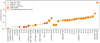 |
Fig. A.1 70 μm flux from Spezzi et al. (2013). Circles indicate detected sources, and the triangles are the upper limits for the non-detections. Red circles indicate sources observed with our ALMA program, and blue squares show the sources that were not detected by our millimeter observations. Finally, the orange squares display the sources that were confirmed as Cha II cluster member by the analysis of Galli et al. (2021). |
Appendix B Cumulative distributions curves
Results of pair comparisons with the logrank test applied on the ratio Mdust/M⋆ for disks moremassive than 1.52 M⊕.
Even though the Kaplan–Meier estimator and the logrank test take into account the non-detections, we performed the analysis considering a common dust mass limit. On Fig B.1, we show the distributions functions of Mdust and Mdust∕M⋆ when considering all systems with disk masses smaller than 1.52 M⊕ (the highest Mdust, min in Table 4) as non-detections. We observe the same ranking in Mdust as in Sect. 4.2. The results of the logrank test are also presented in Table B.1. As expected, they are less statistically different than when the full samples are considered.
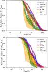 |
Fig. B.1 Cumulative distributions as in Fig. 4 considering disks with smaller masses than 1.52M⊕ as non-detections. We normalized the Mdust distributionsto 1 since the distributions are complete above the 1.52 M⊕ limit. |
References
- Alcalá, J. M., Spezzi, L., Chapman, N., et al. 2008, AJ, 676, 427 [Google Scholar]
- Alcala, J. M., Manara, C. F., Natta, A., et al. 2017, A&A, 600, A20 [NASA ADS] [CrossRef] [EDP Sciences] [Google Scholar]
- Andrews, S. M., & Williams, J. P. 2005, ApJ, 631, 1134 [Google Scholar]
- Andrews, S. M., Rosenfeld, K. A., Kraus, A. L., & Wilner, D. J. 2013, AJ, 771, 129 [NASA ADS] [CrossRef] [Google Scholar]
- Andrews, S. M., Huang, J., Pérez, L. M., et al. 2018, ApJ, 869, L41 [NASA ADS] [CrossRef] [Google Scholar]
- Ansdell, M., Williams, J. P., van der Marel, N., et al. 2016, AJ, 828, 46 [NASA ADS] [CrossRef] [Google Scholar]
- Ansdell, M., Williams, J. P., Manara, C. F., et al. 2017, AJ, 153, 240 [NASA ADS] [CrossRef] [EDP Sciences] [Google Scholar]
- Ansdell, M., Williams, J. P., Trapman, L., et al. 2018, ApJ, 859, 21 [NASA ADS] [CrossRef] [Google Scholar]
- Ansdell, M., Haworth, T. J., Williams, J. P., et al. 2020, AJ, 160, 248 [Google Scholar]
- Ballering, N. P., & Eisner, J. A. 2019, AJ, 157, 144 [Google Scholar]
- Baraffe, I., Homeier, D., Allard, F., & Chabrier, G. 2015, A&A, 577, A42 [NASA ADS] [CrossRef] [EDP Sciences] [Google Scholar]
- Barenfeld, S. A., Carpenter, J. M., Ricci, L., & Isella, A. 2016, AJ, 827, 142 [NASA ADS] [CrossRef] [Google Scholar]
- Beckwith, S., Sargent, A. I., Chini, R., & Gusten, R. 1990, ApJ, 99, 924 [Google Scholar]
- Cazzoletti, P., Manara, C. F., Baobab Liu, H., et al. 2019, A&A, 626, A11 [NASA ADS] [CrossRef] [EDP Sciences] [Google Scholar]
- Cieza, L. A., Padgett, D. L., Allen, L. E., et al. 2009, ApJ, 696, L84 [NASA ADS] [CrossRef] [Google Scholar]
- Cieza, L. A., Ruíz-Rodríguez, D., Hales, A., et al. 2019, MNRAS, 482, 698 [Google Scholar]
- Cox, E. G., Harris, R. J., Looney, L. W., et al. 2017, ApJ, 851, 83 [Google Scholar]
- Dent, W. R. F., Pinte, C., Cortes, P. C., et al. 2019, MNRAS, 482, L29 [Google Scholar]
- Dullemond, C. P., Birnstiel, T., Huang, J., et al. 2018, ApJ, 869, L46 [NASA ADS] [CrossRef] [EDP Sciences] [Google Scholar]
- Dzib, S. A., Loinard, L., Ortiz-León, G. N., Rodríguez, L. F., & Galli, P. A. B. 2018, ApJ, 867, 151 [NASA ADS] [CrossRef] [Google Scholar]
- Eisner, J. A., Arce, H. G., Ballering, N. P., et al. 2018, ApJ, 860, 77 [NASA ADS] [CrossRef] [Google Scholar]
- Facchini, S., van Dishoeck, E. F., Manara, C. F., et al. 2019, A&A, 626, L2 [NASA ADS] [CrossRef] [EDP Sciences] [Google Scholar]
- Fedele, D., van den Ancker, M. E., Henning, T., Jayawardhana, R., & Oliveira, J. M. 2010, A&A, 510, A72 [NASA ADS] [CrossRef] [EDP Sciences] [Google Scholar]
- Feigelson, E. D., & Nelson, P. I. 1985, ApJ, 293, 192 [NASA ADS] [CrossRef] [Google Scholar]
- Gaia Collaboration (Brown, A. G. A., et al.) 2018, A&A, 616, A1 [NASA ADS] [CrossRef] [EDP Sciences] [Google Scholar]
- Gaia Collaboration (Brown, A. G. A., et al.) 2021, A&A, 649, A1 [NASA ADS] [CrossRef] [EDP Sciences] [Google Scholar]
- Galli, P. A. B., Bouy, H., Olivares, J., et al. 2020a, A&A, 634, A98 [CrossRef] [EDP Sciences] [Google Scholar]
- Galli, P. A. B., Bouy, H., Olivares, J., et al. 2020b, A&A, 643, A148 [EDP Sciences] [Google Scholar]
- Galli, P. A. B., Bouy, H., Olivares, J., et al. 2021, A&A, 646, A46 [NASA ADS] [CrossRef] [EDP Sciences] [Google Scholar]
- Geoffray, H., & Monin, J.-L. 2001, A&A, 369, 239 [NASA ADS] [CrossRef] [EDP Sciences] [Google Scholar]
- Grant, S. L., Espaillat, C. C., Wendeborn, J., et al. 2021, ApJ, 913, 123 [NASA ADS] [CrossRef] [Google Scholar]
- Herczeg, G. J., & Hillenbrand, L. A. 2015, ApJ, 808, 23 [Google Scholar]
- Hildebrand, R. H. 1983, QJRAS, 24, 267 [NASA ADS] [Google Scholar]
- Kraus, A. L., Ireland, M. J., Hillenbrand, L. A., & Martinache, F. 2012, ApJ, 745, 19 [NASA ADS] [CrossRef] [Google Scholar]
- Law, C. J., Ricci, L., Andrews, S. M., Wilner, D. J., & Qi, C. 2017, AJ, 154, 255 [NASA ADS] [CrossRef] [Google Scholar]
- Long, F., Pinilla, P., Herczeg, G. J., et al. 2018, ApJ, 869, 17 [NASA ADS] [CrossRef] [Google Scholar]
- Luhman, K. L. 2007, ApJSS, 173, 104 [NASA ADS] [CrossRef] [Google Scholar]
- Mamajek, E. E. 2009, in AIP Conf. Ser., eds. T. Usuda, M. Tamura, & M. Ishii, 1158, 3 [Google Scholar]
- Manara, C. F., Testi, L., Herczeg, G. J., et al. 2017, A&A, 604, A127 [NASA ADS] [CrossRef] [EDP Sciences] [Google Scholar]
- McMullin, J. P., Waters, B., Schiebel, D., Young, W., & Golap, K. 2007, in ASP Conf. Ser., 376, Astronomical Data Analysis Software and Systems XVI, eds. R. A. Shaw, F. Hill, & D. J. Bell, 127 [Google Scholar]
- Mizuno, A., Yamaguchi, R., Tachihara, K., et al. 2001, PASJ, 53, 1071 [NASA ADS] [CrossRef] [Google Scholar]
- Pascucci, I., Testi, L., Herczeg, G. J., et al. 2016, ApJ, 831, 125 [Google Scholar]
- Pecaut, M. J., Mamajek, E. E., & Bubar, E. J. 2012, ApJ, 746, 154 [Google Scholar]
- Ribas, Á., Merín, B., Bouy, H., & Maud, L. T. 2014, A&A, 561, A54 [NASA ADS] [CrossRef] [EDP Sciences] [Google Scholar]
- Ribas, Á., Espaillat, C. C., Macías, E., et al. 2017, ApJ, 849, 63 [NASA ADS] [CrossRef] [Google Scholar]
- Ribas, Á., Espaillat, C. C., Macías, E., & Sarro, L. M. 2020, A&A, 642, A171 [EDP Sciences] [Google Scholar]
- Ruíz-Rodríguez, D., Cieza, L. A., Williams, J. P., et al. 2018, MNRAS, 478, 3674 [NASA ADS] [CrossRef] [Google Scholar]
- Sanchis, E., Testi, L., Natta, A., et al. 2021, A&A, 649, A19 [NASA ADS] [CrossRef] [EDP Sciences] [Google Scholar]
- Sicilia-Aguilar, A., Henning, T., Kainulainen, J., & Roccatagliata, V. 2011, ApJ, 736, 137 [NASA ADS] [CrossRef] [Google Scholar]
- Spezzi, L., Alcalá, J. M., Covino, E., et al. 2008, ApJ, 680, 1295 [NASA ADS] [CrossRef] [Google Scholar]
- Spezzi, L., Cox, N. L. J., Prusti, T., et al. 2013, A&A, 555, A71 [NASA ADS] [CrossRef] [EDP Sciences] [Google Scholar]
- Tazzari, M., Testi, L., Natta, A., et al. 2021, MNRAS, 506, 5117 [NASA ADS] [CrossRef] [Google Scholar]
- Trapman, L., Facchini, S., Hogerheijde, M. R., van Dishoeck, E. F., & Bruderer, S. 2019, A&A, 629, A79 [NASA ADS] [CrossRef] [EDP Sciences] [Google Scholar]
- van der Plas, G., Ménard, F., Ward-Duong, K., et al. 2016, ApJ, 819, 102 [NASA ADS] [CrossRef] [Google Scholar]
- van der Plas, G., Ménard, F., Canovas, H., et al. 2017, A&A, 607, A55 [NASA ADS] [CrossRef] [EDP Sciences] [Google Scholar]
- van Terwisga, S. E., Hacar, A., & van Dishoeck E. F. 2019, A&A, 628, A85 [NASA ADS] [CrossRef] [EDP Sciences] [Google Scholar]
- van Terwisga, S. E., van Dishoeck, E. F., Mann, R. K., et al. 2020, A&A, 640, A27 [NASA ADS] [CrossRef] [EDP Sciences] [Google Scholar]
- Williams, J. P., Cieza, L., Hales, A., et al. 2019, ApJ, 875, L9 [Google Scholar]
- Zucker, C., Speagle, J. S., Schlafly, E. F., et al. 2019, ApJ, 879, 125 [NASA ADS] [CrossRef] [Google Scholar]
- Zurlo, A., Cieza, L. A., Pérez, S., et al. 2020, MNRAS, 496, 5089 [Google Scholar]
See documentation at http://lifelines.readthedocs.io/
All Tables
Results of pair comparisons with the logrank test applied on the ratio Mdust /M⋆.
Results of pair comparisons with the logrank test applied on the ratio Mdust/M⋆ for disks moremassive than 1.52 M⊕.
All Figures
|
Fig. 1 Continuum images ordered by decreasing fluxes. Images are 2.4′′ × 2.4′′, except for Hn 24 where we use 4.8′′ × 4.8′′ to show the secondary source. The beam is shown in the lower left corner of each panel. 3σ and 15σ contours are shown in solid and dashed lines, respectively. The color map is chosen to go from −3 σ to the maximum intensity of each image. |
| In the text | |
|
Fig. 2 Line profiles (left panels), 12CO normalized moment 0 maps (middle panels), and 13CO normalized moment 0 maps (right panels) for the sources detected in 12CO. Each line displays two sources. For each source, we display the continuum contours at 50% of the continuum peak (black line) and the CO contours at 50% of the CO peak (white line) on the CO moment 0 maps. The beam size is shown in the bottom left corner of each panel, along with a white line representing a 0.5′′ scale. On the line profiles plots (left panels), we also show a green vertical line at 3 km s−1, where the cloud absorption is estimated, and the size of the integration range to estimate the 12CO and 13CO fluxes reported in Table 3. The maximum fluxes of each line profile are displayed in the top left side of the panels, colored in blue for 12CO and in red for 13CO. The y ticks of the line profiles mark 0%, 50%, and 100% of the maximum fluxes. |
| In the text | |
|
Fig. 3 Dust masses for the 31 sources in our Cha II sample expressed in Earth masses, ordered by increasing dust mass(Table 2). The black and red squares indicates the sources also detected in 12CO and 13CO, respectively.Round symbols show continuum only detected sources and the downward-facing triangles correspond to 3σ upper limitsfor non-detections. |
| In the text | |
|
Fig. 4 Cumulative distributions functions generated by the Kaplan-Meier estimator. Top: cumulative distribution of the dust mass, normalized by the fraction of detected sources in each star-forming regions. Bottom: cumulative distribution of the dust-to-stellar mass ratio. The bottom distributions include disks not detected in millimeter emission. Those are scattered over the distribution of Mdust /M⋆ (see Sect. 4.2.3). We indicate 1σ confidence intervals. |
| In the text | |
|
Fig. 5 Comparison of the dust mass distributions of different star-forming regions to that of Cha II. pϕ is the probability that the synthetic population drawn from the comparison samples and the reference sample come from the same parent population. f(≤ pϕ) is the cumulative distribution for pϕ resulting from the logrank two-sample test for censored data sets after 104 MC iterations. The vertical lines correspond to pϕ of 0.05 and 0.001, respectively. |
| In the text | |
|
Fig. A.1 70 μm flux from Spezzi et al. (2013). Circles indicate detected sources, and the triangles are the upper limits for the non-detections. Red circles indicate sources observed with our ALMA program, and blue squares show the sources that were not detected by our millimeter observations. Finally, the orange squares display the sources that were confirmed as Cha II cluster member by the analysis of Galli et al. (2021). |
| In the text | |
|
Fig. B.1 Cumulative distributions as in Fig. 4 considering disks with smaller masses than 1.52M⊕ as non-detections. We normalized the Mdust distributionsto 1 since the distributions are complete above the 1.52 M⊕ limit. |
| In the text | |
Current usage metrics show cumulative count of Article Views (full-text article views including HTML views, PDF and ePub downloads, according to the available data) and Abstracts Views on Vision4Press platform.
Data correspond to usage on the plateform after 2015. The current usage metrics is available 48-96 hours after online publication and is updated daily on week days.
Initial download of the metrics may take a while.