| Issue |
A&A
Volume 692, December 2024
|
|
|---|---|---|
| Article Number | A76 | |
| Number of page(s) | 16 | |
| Section | Planets, planetary systems, and small bodies | |
| DOI | https://doi.org/10.1051/0004-6361/202451277 | |
| Published online | 03 December 2024 | |
The GAPS programme at TNG
LXII. Studies of atmospheric FeII winds in ultra-hot Jupiters KELT-9b and KELT-20b using the HARPS-N spectrograph
1
INAF – Osservatorio Astronomico di Padova,
Vicolo dell’Osservatorio 5,
35122
Padova, Italy
2
Space Research Institute, Austrian Academy of Sciences,
Schmiedlstrasse 6,
8042
Graz, Austria
3
INAF – Osservatorio Astronomico di Palermo,
Piazza del Parlamento, 1,
90134
Palermo, Italy
4
University of Palermo, Department of Physics and Chemistry “Emilio Segrè”,
Via Archirafi 36,
Palermo, Italy
5
INAF – Osservatorio Astronomico di Brera,
Via E. Bianchi 46,
23807
Merate, Italy
6
Dipartimento di Fisica e Astronomia “Galileo Galilei” – Università degli Studi di Padova,
Vicolo dell’Osservatorio 3,
35122
Padova, Italy
7
INAF – Osservatorio Astrofisico di Catania,
Via S. Sofia 78,
95123
Catania, Italy
8
INAF – Osservatorio Astrofisico di Arcetri,
Largo Enrico Fermi 5,
50125
Firenze, Italy
9
INAF – Osservatorio Astrofisico di Torino,
Via Osservatorio 20,
10025
Pino Torinese, Italy
10
Dipartimento di Fisica, Università degli Studi di Torino,
via Pietro Giuria 1,
10125
Torino, Italy
11
Fundación Galileo Galilei – INAF,
Rambla José Ana Fernandez Pérez 7,
38712
Breña Baja, Tenerife, Spain
12
Department of Physics, University of Rome “Tor Vergata”,
Via della Ricerca Scientifica 1,
00133
Rome, Italy
13
Max Planck Institute for Astronomy,
Königstuhl 17,
69117
Heidelberg, Germany
★ Corresponding author; This email address is being protected from spambots. You need JavaScript enabled to view it.
Received:
27
June
2024
Accepted:
25
September
2024
Abstract
Ultra-hot Jupiters (UHJs) are gas giant planets orbiting close to their host star, with equilibrium temperatures exceeding 2000 K, and among the most studied planets in terms of their atmospheric composition. Thanks to a new generation of ultra-stable high-resolution spectrographs, it is possible to detect the signal from the individual lines of the species in the exoplanetary atmospheres. We employed two techniques in this study. First, we used transmission spectroscopy, which involved examining the spectra around single lines of Fe II. Then we carried out a set of cross-correlation studies for two UHJs: KELT-9b and KELT-20b. Both planets orbit fast-rotating stars, which resulted in the detection of the strong Rossiter-McLaughlin (RM) effect and center-to-limb variations in the transmission spectrum. These effects had to be corrected to ensure a precise analysis. Using the transmission spectroscopy method, we detected 21 single lines of Fe II in the atmosphere of KELT-9b. All of the detected lines are blue-shifted, suggesting strong day-to-night side atmospheric winds. The cross-correlation method leads to the detection of the blue-shifted signal with a signal-to-noise ratio (S/N) of 13.46. Our results are in agreement with models based on non-local thermodynamical equilibrium (NLTE) effects, with a mean micro-turbulence of νmic = 2.73 ± 1.5 km s−1 and macro-turbulence of νmac = 8.22 ± 3.85 km s−1. In the atmosphere of KELT-20b, we detected 17 single lines of Fe II. Considering different measurements of the systemic velocity of the system, we conclude that the existence of winds in the atmosphere of KELT-20b cannot be determined conclusively. The detected signal with the cross-correlation method presents a S/N of 11.51. The results are consistent with NLTE effects, including means of νmic = 3.04 ± 0.35 km s−1 and νmac = 6.76 ± 1.17 km s−1.
Key words: techniques: spectroscopic / planets and satellites: atmospheres / planets and satellites: individual: KELT-9b / planets and satellites: individual: KELT-20b
© The Authors 2024
 Open Access article, published by EDP Sciences, under the terms of the Creative Commons Attribution License (https://creativecommons.org/licenses/by/4.0), which permits unrestricted use, distribution, and reproduction in any medium, provided the original work is properly cited.
This article is published in open access under the Subscribe to Open model. This email address is being protected from spambots. You need JavaScript enabled to view it. to support open access publication.
1 Introduction
High-resolution spectroscopic observations allow us to differentiate the signals coming from an exoplanet’s atmosphere, its host star, and the Earth’s atmosphere. Hot Jupiters and ultra-hot Jupiters (UHJs) are among the best targets for studying the chemical composition of their atmospheres through the application of both transmission and emission spectroscopy.
Thanks to their short orbital periods and hot extended atmospheres, where the equilibrium temperature (Teq) exceeds 2000 K (Parmentier et al. 2018), UHJs are ideal laboratories for atmospheric studies. Due to their tidally locked nature, which leads to extreme temperature differences between the day and night sides, a different chemical composition on both sides is expected and, in addition, strong day-night side winds are observed, as reported for several UHJs. In theoretical simulations, Helling et al. (2019) demonstrated that clouds cannot form due to the extremely high temperatures observed on the day side of the atmospheres. Furthermore, atoms are found in their ionized state, while molecules, due to their total or partial dissociation, typically have a low abundance (Arcangeli et al. 2018).
In recent years, studies of UHJ atmospheres have been performed using high-resolution transmission and emission spectroscopy, revealing the presence of a diverse range of species, including neutral and ionized atoms, such as Ba II, Ca I, Ca II, Cr I, Cr II, Fe I, Fe II, H I, Mg I, Mg II, Na I, Ni I, Ni II, Rb I, Si I Sm I, Ti I, Ti II, V I, and Y II; for example: MASCARA- 2b/KELT-20b (Casasayas-Barris et al. 2018, 2019; Langeveld et al. 2022; Yan et al. 2019; Cauley et al. 2019 Wyttenbach et al. 2020; Borsa et al. 2021b; Pai Asnodkar et al. 2022; Langeveld et al. 2022; Sánchez-López et al. 2022; Fossati et al. 2023), WASP-12b (Jensen et al. 2018), WASP-33b (Nugroho et al. 2017, Nugroho et al. 2020a; Yan et al. 2021), WASP-121b (Cabot et al. 2020; Borsa et al. 2021a; Young et al. 2024; Maguire et al. 2023), WASP- 189b (Yan et al. 2020, Yan et al. 2022a; Stangret et al. 2022; Prinoth et al. 2022, 2023), and WASP-76b (Seidel et al. 2019; Ehrenreich et al. 2020).
Furthermore, studies of UHJs suggest the presence of a thermal inversion in the middle atmosphere. This phenomenon has been observed in several planets including WASP-33b (Nugroho et al. 2020a; Cont et al. 2022), WASP-103b (Kreidberg et al. 2018), KELT-9b (Pino et al. 2022), and WASP-189b (Yan et al. 2020). These observational results are also supported by forward atmospheric models (e.g., Lothringer et al. 2018; Fossati et al. 2021, 2023), which suggest that the thermal inversion is due to metal line heating, particularly for planets orbiting stars hotter than ≈8300 K that do not present the high-energy (X-ray and extreme ultraviolet) emission responsible for hydrogen photoionization. With respect to the particular cases of KELT-9b and KELT-20b, which are the focus of this work, Fossati et al. (2021, 2023) showed that non-local thermodynamical equilibrium (NLTE) effects magnify the inversion through metal-line absorption of stellar UV radiation. Specifically, NLTE leads to significant Fe II overpopulation and Mg II underpopulation, which respectively drive atmospheric heating and cooling, increasing the magnitude of the thermal inversion. These results are supported by the fact that transmission spectra computed accounting for NLTE effects have been so far the only forward models capable of fitting the observed hydrogen Balmer line profiles of these two UHJs (Fossati et al. 2021, 2023).
In this study, we present an analysis of the chemical composition of two the UHJs KELT-9b and KELT-20b, focusing on the transmission spectroscopic studies of Fe II with high-resolution spectroscopic data. The paper is organized as follows. In Sect. 2 we present a detailed literature review of the studied planets, while in Sect. 3 we describe the observations used in this work. In Sect. 4, the transmission spectroscopy analysis is presented, with the results obtained for KELT-9b and KELT-20b shown in Sects. 5 and 6, respectively. In Sect. 7 we focus on the comparison of the results with atmospheric models. The analysis of the transmission spectrum using the cross-correlation method is described in Sect. 8.
2 Studied planets
KELT-9b is aUHJ (Mp = 2.88 MJ, Rp = 1.936 RJ) with Teq = 3921 K. The planet orbits a bright (V = 7.56 mag) A0-type star in 1.48 days (Gaudi et al. 2017; Borsa et al. 2019). The considered stellar and planetary parameters can be found in the Table 1. The orbital and physical parameters make KELT-9b an ideal candidate for atmospheric studies using transmission and emission spectroscopy. The first detection of the atmospheric signature of KELT-9b was presented by Yan & Henning (2018), revealing an extended atmosphere through the Ha line. Transmission spectroscopic studies focusing on single lines additionally showed the presence of Ca II, Fe II (λ4923.9 Å, λ5018.4, Å, λ5169 Å, λ5197.5 Å, λ5234.6, Å λ5276 Å, λ5316.6 Å, λ5363.9 Å, and λ6456.3 Å), Hβ, Na I (D1 and D2), O I (λ7774. 0 Å triplet), and Pashen β (Yan et al. 2019; Cauley et al. 2019; Turner et al. 2020; Wyttenbach et al. 2020; Borsa et al. 2021b; Pai Asnodkar et al. 2022; Langeveld et al. 2022; Sánchez-López et al. 2022). Emission and transmission spectroscopy studies using the crosscorrelation method have reported the detection of Ca I, Ca II, Cr II, Fe I, Fe II, Mg I, Mg II, Na I, Ni I, Sc II, Si I, Sr II, Tb II, Ti II, and Y II (Hoeijmakers et al. 2018, 2019; Kasper et al. 2021; Pino et al. 2022; Lowson et al. 2023; Ridden-Harper et al. 2023; Borsato et al. 2024, 2023). In addition, using space-based observations, Changeat et al. (2022) and Jacobs et al. (2022) presented the detection of TiO, VO, FeH, and H−.
The first work focusing on the analysis of single Fe II lines, presented by Cauley et al. (2019), described the detection of nine lines with velocity shifts ranging from -1.02 to 3.0 km s−1. The most recent studies presented by Pai Asnodkar et al. (2022) focus on wind measurements in the atmosphere of KELT-9b, concentrating on single lines of Fe II, showing significant day-to-night winds from −4 to −10 km s−1. The substantial differences in the detected wind velocities come from the different choices for the mid-transit time.
In Fig. 1, we present an example for one exposure (close to the mid-transit) of the measurement of the time from the midtransit and the radial velocity of one of the exposures assuming four different literature parameters of T0 and orbital period from Gaudi et al. 2017; Pai Asnodkar et al. 2022; Pino et al. 2022, and Ivshina & Winn 2022. The difference between the exposures used in this work varies from 1.8 to 4.4 km s−1 and 3.95 to 6.01 min from the first published measurements by Gaudi et al. 2017.
KELT-20b (Lund et al. 2017), also known as MASCARA- 2b (Talens et al. 2018), is an UHJ (Mp < 3.51 MJ, Rp = 1.83 RJ) with Teq = 2260 K, orbiting a fast-rotating A-type star in 3.47 days. The stellar and planetary parameters can be found in Table 1. The chemical composition of the atmosphere of KELT-20b has been studied by several groups with low- and high-resolution spectrographs using both transmission and emission spectroscopy. Casasayas-Barris et al. (2018, 2019); Langeveld et al. (2022), and Fossati et al. (2023) presented single line detection of Ca II (λ8498 Å, λ8542 Å, and λ8662 Å), Fe II (λ5018 Å, λ5169 Å, and λ5316 Å), Mg I (λ5173 Å), Na I (D1 and D2), Hα, Hβ, and Hγ. In addition, using the cross-correlation method the existence of Ca II, Cr II, Fe I, Fe II, Na I, Ni I, Ni II, Mg I, and Si I have been reported (Stangret et al. 2020; Nugroho et al. 2020b; Hoeijmakers et al. 2020a; Cont et al. 2022; Yan et al. 2022b; Bello-Arufe et al. 2022; Borsa et al. 2022; Johnson et al. 2023; Kasper et al. 2023; Petz et al. 2024). Evidence of H2O and CO in the emission spectrum was presented by Fu et al. (2022), using observations from TESS, HST WFC3/G141, and the Spitzer 4.5 μm channel.
The first single-line analysis of Fe II lines was presented by Casasayas-Barris et al. (2019), revealing the discovery of three Fe II lines (λ5018 Å, λ5169 Å, and λ5316 Å) using high-resolution observations from the HARPS-N spectrograph, reporting day-side winds of ∼−2.8 km s−1. Pai Asnodkar et al. (2022) presented the detection of three additional Fe II lines (24923.9 Å, λ5276 Å, and λ5363.9 Å). Consistent with the previous works, day-to-night side winds with a blue shift of ∼−2.55 km s−1 were detected.
KELT-9b and KELT-20b are two of the eight UHJs (nine exoplanets in total), where Fe II has been detected in their atmospheres. In Fig. 2, we plot the transmission spectroscopy metrics for all known UHJs (Teq > 2000 K) as a function of their Teq values and the brightness of the host star.
In this work, we focus on the detection of Fe II in the atmosphere of two UHJs KELT-9b and KELT-20b using both singleline analysis and cross-correlation method with high-resolution observations in the visible part of the spectrum.
Physical and orbital parameters of the KELT-9 and KELT-20 systems.
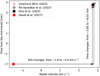 |
Fig. 1 Illustrative example displaying the dependence of time from the mid-transit and the radial velocity of the planet change on the T0 and orbital period (for only one exposure), as calculated by Gaudi et al. 2017, Pai Asnodkar et al. 2022, Pino et al. 2022, and Ivshina & Winn 2022. The values radial velocities of the planet change between 1.8 to 4.4 km s−1 and the time difference from the mid-transit changes from 3.95 to 6.01 min depending on the exposure used in this work, in comparison with the values assuming T0 and period from Gaudi et al. 2017. |
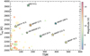 |
Fig. 2 Equilibrium temperature as the function of the transmission spectroscopy metrics for all known ultra-hot Jupiters (Teq > 2000 K). Planets with the Fe II detected in their atmospheres are marked with the star symbol (the list of planets was taken from the ExoAtmospheres database). |
3 Observations
Our work focuses on high-resolution observations of the transits of two exoplanets, KELT-9b and KELT-20b, with the HARPS- N spectrograph (Cosentino et al. 2012, 2014) mounted on the 3.6 m Telescopio Nazionale Galileo (TNG) at the Observato- rio del Roque de los Muchachos (ORM) in La Palma, Spain. HARPS-N is a high-dispersion spectrograph with a resolving power of R ~ 115 000 and continuous wavelength coverage from 3800 to 6900 Å.
We have analyzed six nights of primary transit observations of KELT-9b, two of which were public, and the remaining four were taken as part of the GAPS (Global Architecture of Planetary System, Covino et al. 2013) program. The observing log can be found in Table 2; in brief, all observations cover the orbital phase before, during, and after the transit. The exposure time varies between 300 and 600 s, and the signal-to-noise ratio (S/N), on the spectral order of 53, around the Na I doublet varies between 57.2 and 209. During data analysis, we decided to remove one spectrum from the night of 2018-07-20 and one from the night of 2018-09-01, because of a significantly lower S/N compared to the other spectra taken during the same night. The S/N and airmass changes during the observations are presented in Fig. 3 (top panel), where black crosses indicate the low S/N spectra that were excluded from the analysis.
In the case of KELT-20b, we analyzed six transit observations of HARPS-N, three of which were taken as part of the GAPS collaboration and three were public. The observing log can be found in Table 2. The exposure time varies from 200 to 600 s and the S/N around the Na I doublet varies from 46.6 to 199.9. During the analysis, we removed the spectra from the nights 2018-07-12 and 2022-07-31 with S/N around Na I lower than 60. This removal was not applied to the night of 2022-07-31 due to the lower signal for all data. The S/N and airmass changes during the observations are presented in Fig. 3 (bottom panel).
Observing log of the KELT-9b and KELT-20b transit observations. The table does not include spectra that were excluded from the analysis.
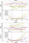 |
Fig. 3 Changes in S/N and airmass during the observations of KELT-9b (upper panel) and KELT-20b (lower panel). The black vertical dotted lines indicate T1 and T4, and the gray vertical dotted lines indicate T2 and T3. The black crosses indicate the low S/N spectra that were excluded from the analysis. |
4 Transmission spectroscopy
In the first step of data analysis, we employed the Spectral Lines Of Planets with python (SLOPpy1, Sicilia et al. 2022) pipeline to correct for sky emission, differential refraction, and telluric lines. The telluric correction was performed with Molecfit (Smette et al. 2015; Kausch et al. 2015), an ESO software tool that fits synthetic transmission spectra to the data in order to correct for atmospheric absorption features. As this step is part of the SLOPpy analysis flow, we refer to Sicilia et al. (2022) for more details. Furthermore, we tested our analysis using spectra non-corrected by tellurics for the following lines: Fe II 24489 Å, 24555 Å, 25018 Å, and 25316 Å (see an example of transmission spectrum with and without correction for KELT-9b in Fig. A.12). In general, due to the fact that the lines in our work lie far away from strong telluric lines, the differences between corrected and uncorrected spectra are negligible.
In the next step, we shifted the spectra to the stellar rest frame using the barycentric correction, as well as the stellar motions around the center of mass using the literature measurements of the semi-amplitude of the radial velocities, K*. The data were not corrected for the systemic velocity (vsys), due to the different values reported in the literature for both KELT-9b and KELT-20b. A detailed discussion can be found in Sects. 5 and 6. The vsys value needs to be calculated with good precision to correct for the center-to-limb variation (CLV) and the Rossiter-McLaughlin (RM) effect and, thus, to accurately calculate the wind in the atmosphere of the exoplanet, which is one of the goals of this work. The calculation of vsys is presented and explained in the next sections of this work. The systemic velocity is constant during the observations, which consequently allows us to apply this correction at every step in the analysis.
In the next step, due to computational limitations, the s1d spectrum was divided into 46 segments and in the following analysis, each of the steps was applied to each segment separately. We normalized the spectrum for each of the segments by the average spectrum over time, following the approach presented by Hoeijmakers et al. (2020b). To this end, for each of the segments, we calculate the mean value of the averaged spectrum, next the averaged spectrum is divided by this value. Then, each of the spectra was divided by the corresponding value from the previous calculations so that all spectra remained at a similar flux level. Next, by looking at the changes of each pixel over time, the outliers that varied more than 3σ from the mean value were linearly interpolated to the nearest pixels. The stellar signal was corrected by dividing all spectra by the master-out spectrum, which was calculated as the average spectrum of all out-of-transit spectra. The remaining residuals were used for the analysis of the single lines of Fe II, as well as for the cross-correlation method presented in Sect. 8.
Here, we examine the Fe II single lines in the transmission spectrum. For each line, we created a residual map which consists of the residuals for each of the orbital phases and the wavelength from ±5 Å from the laboratory wavelength of the line (obtained from the National Institute of Standards and Technology via petitRADTRANS, Mollière et al. 2019). The analysis was conducted separately for each night and subsequently combined, assuming equal weight for each night. In the case of KELT-20b, due to the low S/N of the first and fifth nights, an additional analysis was performed using only the second, third, and fourth nights. However, the results were found to be consistent with those obtained using all nights; thus we present the results using all the nights.
By applying a Markov chain Monte Carlo (MCMC, Foreman-Mackey et al. 2013) algorithm we fitted the planetary signal and the CLV and RM effect simultaneously. In the case of the planetary signal, we assume a Gaussian shape of the signal, which moves with the radial velocity of the planet in its orbit. The velocity of the planet on its orbit vpl assuming circular orbit was calculated as:
 (1)
(1)
where Kp is the semi-amplitude of the exoplanet radial velocity, ø is the orbital phase, and vsys+wind is the velocity of the signal, which consists of the systemic velocity and the velocity of the wind in the atmosphere (vwind), remembering that vsys has not yet been corrected. In addition, using the LDTk tool (Parviainen & Aigrain 2015; Husser et al. 2013), we calculated the limb-darkening coefficient for each star. Then, using PyTransit (Parviainen 2015) assuming the parameters from Table 1, we calculated the transit models. The fitted signal of the planet was then scaled using the transit model.
Both KELT-9b and KELT-20b orbit fast-rotating stars; therefore, a strong RM effect is expected, especially influencing the shape of the Fe II lines, which are also present in the stellar spectra. To correct for this effect together with the CLV, we created models of the CLV and RM effect following Yan et al. (2017) and Yan & Henning (2018), and later used in several works of atmospheric studies such as Casasayas-Barris et al. (2019), Chen et al. (2020), Borsa et al. (2021a), and Stangret et al. (2022). The synthetic spectrum for our planets was computed with Spectroscopy Made Easy (SME, Piskunov & Valenti 2017) using the VALD3 line list (Ryabchikova et al. 2015) and Kurucz ATLAS9 stellar model atmospheres (Castelli & Kurucz 2003). Assuming local thermodynamical equilibrium (LTE) and solar abundance, we calculated models for 21 different limb-darkening angles. Next, we calculated the stellar spectra at the different orbital phases of the planet, keeping in mind that the planet covers different parts of the stellar spectra. In addition, the models were created for several radii of the planet, from 0.7 to 1.5, with a step of 0.1, taking into consideration that the observed radius of the planet depends on the wavelength at which the observations were performed. Finally, all of the spectra were divided by the out-of-transit spectra where we did not expect the influence of the planet on the spectrum, leaving us with the CLV and RM effect at each of the orbital phases and different radii of the planet. The models were then linearly interpolated to the different orbital phases depending on the considered night and planet, and also broadened to the resolution of the HARPS-N spectrograph using instrBroadGaussFast3 from PyAstronomy (Czesla et al. 2019). Finally, the models were interpolated with the third-degree polynomial to the different radii of the planet.
In the MCMC analysis, the CLV and RM effect models were used to fit the radius of the planet depending on the wavelength (Rλ), as well as vsys, where the models were calculated assuming vsys = 0 km s−1 . In the final MCMC, we used 20 walkers and 5000 steps to fit the amplitude, h, Kp, σ, and vsys+wind for the planetary signal and Rλ and vsys using the CLV and RM models. Each of these parameters had a uniform prior. All of the corner plots of the analysis are presented in the appendix.
At the high temperatures found in the atmospheres of UHJs, Fe II presents strong absorption features. In this work, to identify the possible signals in the transmission spectrum, we created a synthetic model of Fe II for a uniform atmospheric temperature of 4000 K with PetitRadTrans. Next, we created a “fast” transmission spectrum (TS) assuming theoretical Kp, literature vsys, and Rλ = Rp. Then, we shortened the list of possible detections by visual inspection. For each of the lines, nights, and combinations of nights for each planet, we performed the MCMC analysis described in Sect. 4.
Tables 3 and 4 present a brief overview of the detected and non-detected lines for each night, as well as for the nights combined for KELT-9b and KELT-20b, respectively. The lines for which all the parameters converged in the MCMC analysis are represented in green. Those for which only one parameter did not converge in the MCMC analysis are marked in yellow, while non-detections (i.e., more than two parameters were not converged in the MCMC analysis) are marked in red. In the case of single-night analysis, the results are presented for visualization purposes only.
5 Detected lines – KELT-9b
Our analysis led to the detection of 21 Fe II single lines in the atmosphere of the UHJ KELT-9b. The list of detected lines and the fitted parameters are presented in Table 5, and all transmission spectra of the considered lines are plotted in Fig. 4. All detected lines are simultaneously presented by D’Arpa et al. (2024) using the same data set, but using significantly different methodology. In our work, we focus on the analysis using the MCMC method, with several parameters fitted simultaneously. A detection is reported only when all the parameters have been converged in the MCMC analysis. In our analysis, we are focusing exclusively on the unblended lines of Fe II. Four lines detected by D’Arpa et al. (2024) were excluded from our analysis because, for the Fe II λ4296 Å line, the MCMC did not converge for both Kp and amplitude, the Fe II λ 4549 Å line is blended with a strong Ti II line, the Fe II 24303 Å line blends with a Fe I line, and the Fe II 26456 Å line may potentially blend with two additional lines to the extent that their RM effect ends up covering the Fe II line.
In Fig. 5, we present an example of the MCMC and TS analysis carried out for the Fe II λ5018.4 Å line. The figure consists of a residual map in the stellar rest frame, with a visible signal coming from the planetary atmosphere (light-tilted signal) and the RM effect (dark vertical signal). In the second panel, we show the best-fitted model of the planetary signal and RM and CLV effect using the MCMC analysis described in Sect. 4. The residual map after correcting for the RM and CLV effect is presented in the third panel. The transmission spectrum compared to the best-fitting Gaussian model, synthetic atmospheric spectrum computed assuming local-thermodynamic equilibrium (LTE) and accounting for non-local thermodynamic equilibrium (NLTE) effects (see Sect. 7) is shown in the fourth panel. The corner plots of the MCMC analysis and the transmission spectrum for all the studied lines can be found in the appendix (Figs. A.2-A.7 for TS, and Figs. A.8-A.18 for corner plots, available on Zenodo).
In Fig. 6 we present the amplitude as the function of the FWHM (upper panel) and Kp as the function of wavelength (lower panel) for all of the detected Fe II lines. The mean values of FWHM and Kp are 16.87 ± 4.75 km s−1 and 236.4 ± 9.0 km s−1, respectively, where the latter is consistent with the Kp obtained from the orbital parameters, that is Kp = 246.99 ± 5.72 km s−1.
In Fig. 7, we present the values of vsys+wind and vsys as a function of the wavelength of the detected line, and vwind as a function of the amplitude of the detected signal. The mean measured vsys = −21.61 ± 0.77 km s−1 is slightly larger than those reported in the literature by Hoeijmakers et al. (2019, -17.74 ± 0.11 km s−1), Borsa et al. (2019, -19.819 ± 0.024 km s−1), and Gaia (−20.22 ± 0.49 km s−1). By calculating the velocity of the atmospheric winds and considering the vsys value from our MCMC analysis, we were able to detect atmospheric winds in the atmosphere of KELT-9b of vwind = −3.41 ± 1.56 km s−1. Given that the vsys calculated in our work is the lowest among those presented in the literature, it can be stated with confidence that the KELT- 9b has strong atmospheric blue-shifted day-to-night side winds with a minimum velocity of -3.41 km s−1.
As previously stated, the final velocity of the wind is dependent on the different literature values of T0 and the period. We repeated the calculation around Fe II 5018.4 Å, using the values presented in Gaudi et al. (2017), Pai Asnodkar et al. (2022), Pino et al. (2022), and Ivshina & Winn (2022). The transmission spectrum can is shown in Fig. 8. The only discrepancy is observed in the values derived from Gaudi et al. (2017), where the position of the line is approximately 6 km s−1 away. However, this discrepancy is not reflected in the line position for values derived from the remaining literature. As the values obtained using TESS data are in alignment with each other, we have determined that these are the most precise.
Detected and non-detected Fe II lines for KELT-9b for each of the nights. Detected lines are colored green, non-detected lines are colored red, and possible detections are colored yellow.
6 Detected lines: KELT-20b
The analysis of six transits of KELT-20b led to the detection of 17 single lines of Fe II. The list of detected lines and the fitted parameters are presented in Table 6 and the transmission spectra of the studied lines are presented in Fig. 9. The lines λ5018 Å, λ5169 Å, and λ5316 Å were previously detected by Casasayas-Barris et al. (2019), while the detection of the remaining lines is presented here for the first time.
Similarly to Fig. 5, in Fig. 10 we present the MCMC and TS analysis around the Fe II λ5018.4 Å line. The RM effect is visible as a dark tilted signal, while the atmospheric detection is a light slightly tilted signal. The corner plots of the MCMC analysis and the transmission spectrum for all the studied lines can be found in the appendix (Figs. B.1–B.6 for TS, and Figs. B.7–B.17 for corner plots, available on Zenodo.)
In Fig. 11 we present the amplitude of the absorption signal as a function of FWHM and Kp as a function of the wavelength of the detected lines. We find an average FWHM value of 8.27 ± 3.74 km s−1 and Kp of 155.8 ± 21.2 km s−1, where the latter is consistent with the Kp obtained considering the orbital parameters, namely, Kp = 169.34 ± 6.56 km s−1.
In Fig. 12 we present the obtained vsys+wind and vsys values as a function of the wavelength of the detected lines, and vwind as a function of the amplitude of the detected signal. We obtain an average vsys value of −24.52 ± 0.40 km s−1. Due to the discrepancy among vsys values present in the literature, namely −23.3 ± 0.3 km s−1 (Lund et al. 2017), −21.3 ± 0.4 and −21.07 ± 0.03 km s−1 (Talens et al. 2018), −22.06 ± 0.35 and −22.02 ± 0.47 km s−1 (Nugroho et al. 2020b), −24.48 ± 0.04 km s−1 (Rainer et al. 2021), and −26.78 ± 0.71 km s−1 (Gaia), it is difficult to determine the optimal value and correct for vsys . Therefore, the existence or non-existence of winds in the atmosphere of this planet cannot be reliably determined. The mean value of vsys+winds obtained from the MCMC analysis is −23.73 ± 0.84 km s−1. Assuming the value of vsys calculated in this work, we obtain vwind = 0.8 ± 0.8 km s−1, which is consistent with the non-detection of atmospheric winds.
Detected Fe II lines in the atmosphere of KELT-9b.
Detected Fe II lines in the transmission spectrum of KELT-20b.
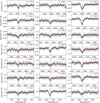 |
Fig. 4 Transmission spectra for all lines detected in KELT-9b (gray dots). Black dots indicate the binned transmission spectrum with a step of 0.1 Å. The red dashed lines represent the best Gaussian fit of the planetary signal from the MCMC analysis. |
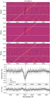 |
Fig. 5 The results of the analysis of the Fe II line at λ5018.4 Å for KELT-9b. Top panel: residual map in the stellar rest frame. The light- tilted signal is the atmospheric signal of Fe II, while the dark almost vertical signal is the RM effect. The white horizontal lines indicate the start and end of the transit, while the tilted white line indicates the expected trace of the Fe II line considering velocities coming from the planet’s atmosphere, assuming vsys = −21.61 km s−1 as the average vsys from our analysis. Second panel: best-fit model of the planetary signal and of the RM and CLV effects. Third panel: same as the top panel, but with the RM and CLV effects corrected. Fourth panel: transmission spectrum of the detected line (gray dots). The black dots indicate the binned transmission spectrum with a step of 0.1 Å. The red line is the best Gaussian fit of the planetary signal derived from the MCMC analysis, the blue line shows the LTE model, and the green line indicates the NLTE model. Bottom panel: residuals after removing Gaussian fit from the TS. |
7 NLTE transmission spectroscopic models
Fossati et al. (2021, 2023) showed that NLTE effects impact significantly the temperature-pressure (TP) profile and transmission spectrum of both KELT-9b and KELT-20b. In particular, NLTE effects increase by more than 3000 K the temperature in the middle and upper atmosphere, compared to TP profiles computed assuming LTE. Generally NLTE effects lead to stronger absorption in transmission spectra, except for some typically weak lines mostly of neutral iron and calcium.
We compared the results of our observations with the synthetic NLTE transmission spectra of Fossati et al. (2021, 2023). The considered TP profiles are the same as those presented by Fossati et al. (2021) for KELT-9b and by Fossati et al. (2023) for KELT-20b. Each of the two TP profiles has been computed employing the HELIOS code (Malik et al. 2017, 2019, see also Fossati et al. 2021 for the additionally considered opacities) in the lower atmosphere (pressures higher than about 0.1 mbar) and the CLOUDY NLTE radiative transfer code (version 17.03; Ferland et al. 2013, 2017), through the CLOUDY for Exoplanets (CfE) interface (Fossati et al. 2021; Young et al. 2024), at lower pressures, and assuming solar abundances. This separation was applied because HELIOS does not account for NLTE effects that are relevant in the middle and upper atmosphere; whereas CLOUDY, which considers NLTE effects, is unreliable at densities greater than 1015 cm−3 (see Ferland et al. 2017, for more details). Fossati et al. (2021, 2023) presented also LTE TP profiles that have been computed in the same way, but assuming LTE for the CLOUDY calculations. Transmission spectra have been computed on the basis of the TP and abundance profiles obtained from the LTE and NLTE calculations following the procedure described by Young et al. (2020) and Fossati et al. (2020). We remark that the NLTE transmission spectra were computed by employing the NLTE TP profiles and enabling NLTE in the CLOUDY calculations. The LTE transmission spectra have been computed using the LTE TP profiles and imposing the LTE assumption for the CLOUDY transmission spectra calculation. Furthermore, these are forward self-consistent models that do not employ free parameters that are tweaked to fit the observations (i.e., the computation of the TP profiles and of the synthetic spectra is agnostic of the observations and employs exclusively the system parameters and the stellar spectral energy distribution as input). All details of the atmospheric structure (i.e., TP and abundance profiles) and transmission spectra calculations for KELT-9b and KELT-20b can be found in Fossati et al. (2021, 2023), respectively.
As in previous works (Borsa et al. 2021b), we broadened the NLTE synthetic spectra accounting for microturbulence velocity (νmic; added in quadrature to the thermal velocity), macroturbulence velocity (νmac), and planetary rotation. This was done with the assumption a tidally locked planet (i.e., vrot = 6.64 km s−1 for KELT-9b and vrot = 2.73 km s−1 for KELT-20b), using fastRotBroad from PyAstronomy. In particular, the synthetic spectra were computed for νmic values of 1, 2, 3, 4, 6, 8, 10, 12, 14, and 18 km s−1, with the transmission spectra for in-between νmic values obtained through interpolation using a fifth-degree polynomial.
We compared the observed and NLTE synthetic line profiles employing an MCMC algorithm to finally extract for each detected line the best fitting νmic−νmac pair. We ran the MCMC employing 10 000 steps and 20 walkers, assuming uniform priors on νmic and νmac in the 0–14 and 0–25 km s−1 ranges, respectively, and leaving the line center as a free parameter (see D’Arpa et al. 2024, for more details). The best fitting νmic and νmac values are listed in Tables 5 and 6, while the relative corner plots obtained from the MCMC fitting are displayed in the appendix (Figs. A.19 and A.20 for KELT-9b, and Figs. B.18 and B.19 for MASCARA-2b).
In the case of KELT-9b, we find average νmic and νmac values of 2.7 ± 1.6 km s−1 and 8.2 ± 3.7 km s−1, respectively, which agree within 1σ with what independently obtained in previous studies by Borsa et al. (2021b, νmic = 3.0 ± 0.7 km s−1, νmac = 13 ± 5 km s−1), and D’Arpa et al. (2024) (νmac = 3.0 ± 0.3 km s−1, νmac = 6.8 ± 1.2 km s−1) employing the same models, but considering different spectral lines and/or different data analysis methods. In Fig. 13, we present the fitted values of νmic and νmic for each of the detected lines.
Also, in the case of KELT-20b, we find that the best fitting NLTE models are for non-zero microturbulence and/or macroturbulence values and on average we find νmic =1.4 ± 1.3 km s−1 and νmac = 5.1 ± 3.1 km s−1. Figure 14 shows the fitted values of νmac and νmac for each of the detected lines.
In Fig. 15, we show as an example the observed transmission spectra compared to the LTE and NLTE synthetic profiles for KELT-9b and KELT-20b. In the case of KELT-9b, the NLTE profiles reproduce significantly better the observed features compared to the LTE profiles. In the case of KELT-20b, NLTE effects seem to have less of an impact on the line profiles, particularly for weak lines; whereas the difference between the LTE and NLTE features is larger for stronger lines, for which the NLTE synthetic spectra allow for a better ft to the observations.
These results support those of Fossati et al. (2021, 2023), who found that transmission spectra computed accounting for NLTE effects fit significantly better the hydrogen Balmer line profiles compared to those obtained assuming LTE. Altogether, these results indicate that the higher middle and upper atmospheric temperature obtained when accounting for NLTE effects is a better representation of the planetary atmosphere. The good fit obtained by the NLTE transmission spectra of the metal lines presented here is a further indication that the NLTE model is capable to adequately reproduce not only the TP profile, but also the Fe II ionisation fraction and level population across the atmosphere. In turn, this supports the conclusion that in KELT-9b and KELT-20b, the temperature inversion is driven by metal-line heating; thus, NLTE effects play the role of over-populating the lower energy levels of Fe II and under-populating Mg II, which are responsible for driving most of the heating and cooling, respectively.
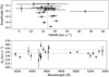 |
Fig. 6 Amplitude, Kp, and FWHM of the Fe II lines detected in atmosphere of KELT-9b. Top panel: amplitude of the transmission signal detected from the MCMC analysis for each of the detected lines as the function of their FWHM. The red vertical dashed line indicates the mean value of FWHM. Bottom panel: Kp as a function of wavelength of the detected lines. The red horizontal dashed line indicates the mean Kp value, while the gray horizontal dashed line indicates the theoretical value. |
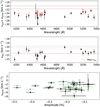 |
Fig. 7 vsys+wind and vsys of the Fe II lines detected in atmosphere of KELT-9b. Top panel: fitted vsys+wind for each of the detected lines. The red dots represent the results of D’Arpa et al. (2024). Middle panel: fitted vsys for each of the detected lines. The red dashed horizontal lines indicate the mean value of the vsys = −21.61 ± 0.77 km s−1, while the grey horizontal dashed lines indicate literature vsys values: −17.74 ± 0.11 km s−1 (Hoeijmakers et al. 2019), −19.819 ± 0.024 km s−1 (Borsa et al. 2019), and −20.22 ± 0.49 km s−1 (Gaia). Bottom panel: vwind versus amplitude plot, where green points represent the values calculated by correcting the fitted vsys+wind by the mean vsys and the black points represent the values corrected by vsys fitted for each of the lines separately. |
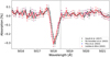 |
Fig. 8 Transmission spectrum around the Fe II 5018.4 Å line in the atmosphere of KELT-9b for T0 and period from Gaudi et al. (2017) (black dots), Pai Asnodkar et al. (2022) (green dots), Pino et al. (2022) (blue points), and Ivshina & Winn (2022) (red points). The black vertical line represents the theoretical position of the studied line. Blue and green points are indistinguishable from the red and black points. |
8 Cross-correlation analysis of the Fe II lines
In addition to transmission spectroscopy around single lines, for both planets, we applied the cross-correlation (CC) method to the available data sets. Following the data reduction steps described in Sect. 4, we cross-correlated the residuals with synthetic models of Fe II. The CC was performed with crosscorrRV from PyAstronomy for each order and each orbital phase separately from −200 to 200 km s−1 with a step size of 0.8 km s−1.
Synthetic LTE models of Fe II were created with PetitRadTrans (Mollière et al. 2019) assuming an isothermal pressure-temperature profile at T = Teq (see Table 1), solar abundances (Asplund et al. 2009), and a cloud layer at P0 = 1 mbar to simulate the continuum opacity produced by H-. (e.g., Hoeijmakers et al. 2019, Stangret et al. 2022, Borsa et al. 2021a). The CC was performed for three different synthetic models, one consisting of all the lines from PetitRadTrans, the second consisting only of lines detected by single-line analysis, and a third one consisting only the lines not detected by single-line analysis. The models computed for KELT-9b and KELT-20b are shown in Fig. 16 (right panel).
Due to the strong influence of the RM effect on each of the Fe II lines, it was necessary to correct the CC maps from this effect. In the first step, we cross-correlated the models of RM and CLV effects with the synthetic models of Fe II. This method turned out to be insufficient in our case, and thus we decided to correct the RM and CLV effects by fitting a Gaussian to the visible structures coming from these effects. Given that the RM effect produces different structures in the CC maps for the two planets, in the case of KELT-9b, we removed the RM signal around −100, −40, 20, and 90 km s−1. Then, in the case of KELT-20b, we removed the RM signal only from -150 to 100 km s−1.
In the next step, we moved the residuals to the planetary rest frame assuming vsys = 0 km s−1 and Kp in the range of 0300 km s−1, where the planetary signal is expected to have its maximum near the theoretical Kp and vsys. Then, after co-adding the in-transit residuals (T1 – T4), we find the best Kp and calculate the S/N plot by dividing the results by the standard deviation calculated away from the expected planetary signal (−200 to -100 km s−1 and 100 to 200 km s−1).
In the top panels of Fig. 17, we present the CC analysis for KELT-9b. The left panel shows the CC residual maps, where the vertical bright signals around -50 km s-1 and 90 km s−1, and the darker signal around −120 km s−1 are the CLV and RM effects. The planetary signal is visible as a tilted dark signal following a red tilted dashed line, which indicates the theoretical radial velocity of the planetary signal. The two horizontal red dashed lines indicate T1 and T4. In the second panel, we present the residual maps after correcting for the CLV and RM effects. In the third panel, we present the Kp map calculated for Kp ranging from 0 to 300 km s−1. The Fe II signal was detected with S/N = 27.02 ± 0.92 and vsys+wind = −25.06 ± 0.10 km s−1 for the CC computed considering all lines, with S/N = 21.97 ± 0.74 and vsys+wind = −24.88 ± 0.11 km s−1 considering the lines detected in the single-line analysis, and with S/N = 8.06 ± 0.27 and vsys+wind = −25.72 ± 0.44 km s−1 considering the lines not detected in the single-line analysis. We successfully identified the signal from the lines not detected in the single-line analysis using the cross-correlation method, although the signal was much weaker than the one coming from the detected lines. This indicates that the main contributors to the cross-correlation analysis were the lines that were detected also through single-line analysis.
In the bottom row of Fig. 17, we present the cross-correlation results for KELT-20b. The signal was detected with S/N = 11.51 ± 0.46 and vsys+wind = −24.27 ± 0.13 km s−1 for the CC computed considering all lines, with S/N = 11.00 ± 0.44 and vsys+wind = −24.32 ± 0.12 km s−1, considering the lines detected in the single-line analysis, and with S/N = 6.98 ± 0.55 and vsys+wind = −25.19 ± 1.04 km s−1 considering the lines not detected in the single-line analysis. Similarly to KELT-9b, the main contributors to the CC signal are the lines detected with the single-line analysis.
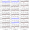 |
Fig. 9 Transmission spectra for all the lines detected in KELT-20b (gray dots) and the transmission spectra around the non-detected lines are marked with blue dots. Dark dots indicate the binned transmission spectrum with a step of 0.1 Å. The red dashed lines represent the best fit of the planetary signal from the MCMC analysis. |
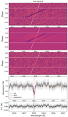 |
Fig. 10 Same as Fig. 5, but for KELT-20b. In the top panel, the RM effect is a tilted dark signal and the planetary signal from Fe II is a bright vertical signal. |
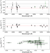 |
Fig. 12 Same as Fig. 7, but for KELT-20b. In the upper panel, the green points represent the measurement obtained by Casasayas-Barris et al. (2019). In the middle panel, we plot several literature systemic velocities with gray horizontal lines: −23.3 ± 0.3 km s−1 (Lund et al. 2017), -21.3 ± 0.4 (Talens et al. 2018), −22.06 ± 0.35 km s−1 (Nugroho et al. 2020b), −24.48 ± 0.04 km s−1 (Rainer et al. 2021), and −26.78 ± 0.71 km s−1 (Gaia). The red horizontal line indicates the mean vsys value of −24.52 km s−1 derived in this work. |
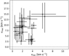 |
Fig. 13 Best-fitting νmic and νmic values obtained for each of the Fe II lines detected in the atmosphere of KELT-9b. |
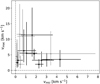 |
Fig. 14 Same as Fig. 13, but for KELT-20b. The values for which both νmic and νmac are consistent with 0 km s−1 or could not be determined are plotted with grey color. |
9 Planetary radius
We employ two distinct methodologies for determining the radius of the planet from the detected lines. In the first methodology, we concentrate on the detected signal from the planet, following the approach of Chen et al. (2020) to calculate the effective radius of the planet (hereafter, Reff). Using the amplitude of the detected signal, we considered Reff /Rp = (δ + h)/δ, where h is the line contrast and δ is (Rp/R*)2 from Table 1. The measured average values are Reff = 1.15 ± 0.07 Rp for KELT-9b and Reff = 1.08 ± 0.04 Rp for KELT-20b. In the bottom panels of Figs. 18 and 19, we present the obtained Reff values as a function of wavelength for all lines detected through the single-line analysis.
In the second methodology, we focused on the detected RM and CLV effect, disregarding the signal coming from the planet. Here, the radius of the planet was calculated by fitting the modeled RM and CLV effect, which were calculated assuming different radii of the planet (hereafter Rλ). The top plots of Figs. 18 and 19 present the Rλ as a function of wavelength for all detected lines.
This method allowed us to find the optimal strength of the RM and CLV effect to clear the map from the effects and, thus, detect weaker lines. For both planets, we find that the radius of the planet (Rλ), as measured using the RM effect, exhibits a linear trend with wavelength. Furthermore, some of the calculated radii were found to be smaller than 1 Rp. The same analysis was repeated using stellar models computed with TurboSpectrum (Plez 2012), presenting a similar behavior (see Fig. A.21 for KELT-9b). As discussed by Casasayas-Barris et al. (2019), where the radius was fitted using a similar methodology focusing on the RM and CLV models, the discrepancy can be attributed to a number of factors. Firstly, the models depend on several parameters, such as Teff, log g, and [Fe/H], where their uncertainties could lead to significant differences among the stellar models. We expect that NLTE effects in both KELT-9 and KELT-20 do not play a significant role in shaping the stellar spectra (e.g., Fossati et al. 2009). However, the models used in the analysis, which assumed an LTE atmosphere of those stars, could potentially introduce a minor additional uncertainty to the overall strength of the effect. Consequently, the collective impact of all uncertainties could result discrepancies in the planetary radius. Furthermore, as seen for example in Fig. A.21, the observed trend appears to be linear.
Here, it is crucial to stress that the obtained Rλ values should not be interpreted as the physical parameter of the planet, but as a scaling factor for the RM and CLV effect. Furthermore, we want to show that because the scaling factor is different for different lines, the RM and CLV effects cannot be corrected for the CC maps without considering an additional scaling factor and/or scaling the strength depending on wavelength, which would require further investigation. Also, we strongly encourage future analyses of the planetary signal to fit the RM and CLV models in the 2D maps. This will ensure that the effects are not under- or overcorrected.
10 Conclusions
In this work, we focused on the two ultra-hot Jupiters KELT-9b and KELT-20b, presenting single-line detections and crosscorrelation analysis of Fe II. We combined six transit observations for each of the planets obtained with the HARPS-N high-resolution spectrograph.
In the case of KELT-9b, using single-line analysis, we detected 21 separated lines of Fe II, with a mean vwind of -3.41 ± 1.56 km s−1 . The blue-shifted lines can indicate the existence of day-to-night winds. In addition, we measured a vsys of −21.61 ± 0.77 km s−1. With the cross-correlation method, we detected the Fe II signal at the level of S/N = 27.02. Additionally, we show that atmospheric models accounting for NLTE effects fit the observations significantly better, as compared to models computed assuming LTE. On the basis of the NLTE models, we obtained νmic = 2.7 ± 1.6 km s−1 and νmac = 8.2 ± 3.7 km s−1, in agreement with previous works.
In the transmission spectrum of KELT-20b, we identified 17 single lines of Fe II. With the measurements of vsys using MCMC fitting (vsys = −24.52 ± 0.40 km s−1) and comparing our results with the literature, it is not clear if the atmospheric signal can conclusively lead to the detection of atmospheric winds. Further studies are required to achieve more precise measurements of vsys. The cross-correlation analysis has revealed a strong detection of Fe II in the atmosphere of KELT-20b with an S/N of 11.51. Similarly to KELT-9b, the observations support models computed considering NLTE effects, from which we obtained νmic = 1.4 ± 1.3 km s−1 and νmac = 5.1 ± 3.1 km s−1.
The analysis of the systemic velocity focused on the analysis of the RM effect. As mentioned in Sect. 4, we modeled the RM and CLV effects assuming vsys = 0.0 km s−1, and during the MCMC analysis we found the best vsys for each of the lines. In the case of KELT-9b, we find an average vsys value of −21.61 ± 0.77 km s−1. The literature values presented by Hoeijmakers et al. (2019), Borsa et al. (2019), and Gaia are -17.74 ± 0.11 km s−1, −19.819 ± 0.024 km s−1, and −20.22 ± 0.49 km s−1, respectively. Depending on which vsys is considered for the correction of the wind velocity, we obtain average wind velocities ranging between −7.2 km s−1 and −4.2 km s−1.
For KELT-20b the obtained mean value of vsys is −24.63 km s−1. The literature measurements presented in the past were −23.3 km s−1 (Lund et al. 2017), -21.3 (Talens et al. 2018), −22.06 km s−1 (Nugroho et al. 2020b), −24.48 km s−1 (Rainer et al. 2021), and −26.78 km s−1 (Gaia). These values are inconsistent among each other. Our measurements are comparable to the values obtained by Rainer et al. (2021) using the same dataset from HARPS-N, which leads to the detection of red-shifted winds of 1.12 km s−1. When considering all the literature vsys values, vwinds varies from −2.21 km s−1 to 3.27 km s−1. In the case of KELT-20b, precise measurements of vsys are necessary to confirm the existence of atmospheric winds.
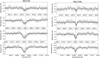 |
Fig. 15 Transmission spectra of the Fe II lines at λ4522 Å, λ4583 Å, λ5018 Å, and λ5169 Å for KELT-9b (left column) and KELT-20b (right column) in comparison to the LTE (blue) and NLTE (green) synthetic profiles computed for the best fitting νmic and νmac values. The red line is the best Gaussian fit of the planetary signal. |
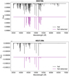 |
Fig. 16 Synthetic transmission spectra computed considering only Fe II for KELT-9b (top panel) and KELT-20b (bottom panel). The black lines are for models created with PetitRadTrans considering all lines, while the purple lines are for models computed considering only the lines detected through the single-line analysis. |
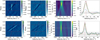 |
Fig. 17 Cross-correlation results for KELT-9b (top panels) and KELT-20b (bottom panels) using all Fe II lines. Left column: cross-correlation residual maps, where the lbright tilted signal is the RM effect, the dark signal is the Fe II atmospheric signal, the red horizontal dashed lines indicate the T1 and T4, and the dashed tilted line represents the expected velocity of the planet where for visualization reasons we assumed vsys equal to the average vsys from the single line analysis. Center-left column: same as the maps in the first column, but after correcting for the RM effect. Center-right column: Kp maps in the range of Kp from 0 to 300 km s−1, where the two horizontal gray dashed lines indicate the theoretical Kp and the best Kp values, respectively, and the vertical gray dashed line indicates the mean vsys value from the single line analysis. Right column: S/N for the best Kp value (black line), fitted Gaussian function (red dashed line), S/N obtained using only the lines detected in the single-line analysis (green line), and S/N obtained using only the lines not detected in the single-line analysis (blue line). The black dashed vertical line indicates the mean vsys value and the red vertical line indicates the velocity of the signal from the Gaussian fit. |
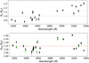 |
Fig. 18 Rλ and Reff of the Fe II lines detected in atmosphere of KELT- 9b. Top panel : fitted Rλ for each of the lines. The dashed horizontal line indicates Rλ = RP. Bottom panel : calculated Reff values using the amplitude of the detected signal for each of the lines (black dots) and the values obtained by D’Arpa et al. (2024) (green dots). |
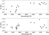 |
Fig. 19 Same as Fig. 18, but for KELT-20b. The green dots in the top panel represent the measurements obtained by Casasayas-Barris et al. (2019) through fitting the strength of the RM effect. |
Data availability
An extended version of the manuscript, with an appendix including Figs. A.1-A.21 and Figs. B.1-B19, can be found on Zenodo https://zenodo.org/records/13881142.
Acknowledgements
The authors and, in particular, M.S. acknowledge the support of the PRIN INAF 2019 through the project “HOT-ATMOS”. This work made use of PyAstronomy (Czesla et al. 2019) and the VALD database, operated at Uppsala University, the Institute of Astronomy RAS in Moscow, We acknowledge the use of the ExoAtmospheres database during the preparation of this work The authors also acknowledge financial contribution from INAF GO Large Grant 2023 GAPS-2 and from the European Union - Next Generation EU RRF M4C2 1.1 PRIN MUR 2022 project 2022CERJ49 (ESPLORA). We acknowledge the Italian Center for Astronomical Archive https://www.ia2.inaf.it/ for providing technical assistance, services and supporting activities of the GAPS collaboration. L.M. acknowledges financial contribution from PRIN MUR 2022 project 2022J4H55R. TZi acknowledges support from CHEOPS ASI-INAF agreement no. 2019-29-HH.0, NVIDIA Academic Hardware Grant Program for the use of the Titan V GPU card and the Italian MUR Departments of Excellence grant 2023-2027 “Quantum Frontiers”. Part of the research activities described in this paper were carried out with contribution of the Next Generation EU funds within the National Recovery and Resilience Plan (PNRR), Mission 4 − Education and Research, Component 2 − From Research to Business (M4C2), Investment Line 3.1 − Strengthening and creation of Research Infrastructures, Project IR0000034 − “STILES − Strengthening the Italian Leadership in ELT and SKA”.
References
- Arcangeli, J., Désert, J.-M., Line, M. R., et al. 2018, ApJ, 855, L30 [Google Scholar]
- Asplund, M., Grevesse, N., Sauval, A. J., & Scott, P. 2009, ARA&A, 47, 481 [NASA ADS] [CrossRef] [Google Scholar]
- Bello-Arufe, A., Buchhave, L. A., Mendonça, J. M., et al. 2022, A&A, 662, A51 [NASA ADS] [CrossRef] [EDP Sciences] [Google Scholar]
- Borsa, F., Rainer, M., Bonomo, A. S., et al. 2019, A&A, 631, A34 [NASA ADS] [CrossRef] [EDP Sciences] [Google Scholar]
- Borsa, F., Allart, R., Casasayas-Barris, N., et al. 2021a, A&A, 645, A24 [EDP Sciences] [Google Scholar]
- Borsa, F., Fossati, L., Koskinen, T., Young, M. E., & Shulyak, D. 2021b, Nat. Astron., 6, 226 [Google Scholar]
- Borsa, F., Giacobbe, P., Bonomo, A. S., et al. 2022, A&A, 663, A141 [NASA ADS] [CrossRef] [EDP Sciences] [Google Scholar]
- Borsato, N. W., Hoeijmakers, H. J., Prinoth, B., et al. 2023, A&A, 673, A158 [NASA ADS] [CrossRef] [EDP Sciences] [Google Scholar]
- Borsato, N. W., Hoeijmakers, H. J., Cont, D., et al. 2024, A&A, 683, A98 [NASA ADS] [CrossRef] [EDP Sciences] [Google Scholar]
- Cabot, S. H. C., Madhusudhan, N., Welbanks, L., Piette, A., & Gandhi, S. 2020, MNRAS, 494, 363 [Google Scholar]
- Casasayas-Barris, N., Pallé, E., Yan, F., et al. 2018, A&A, 616, A151 [NASA ADS] [CrossRef] [EDP Sciences] [Google Scholar]
- Casasayas-Barris, N., Pallé, E., Yan, F., et al. 2019, A&A, 628, A9 [NASA ADS] [CrossRef] [EDP Sciences] [Google Scholar]
- Castelli, F., & Kurucz, R. L. 2003, in Modelling of Stellar Atmospheres, 210, eds. N. Piskunov, W. W. Weiss, & D. F. Gray, A20 [NASA ADS] [Google Scholar]
- Cauley, P. W., Shkolnik, E. L., Ilyin, I., et al. 2019, AJ, 157, 69 [Google Scholar]
- Changeat, Q., Edwards, B., Al-Refaie, A. F., et al. 2022, ApJS, 260, 3 [NASA ADS] [CrossRef] [Google Scholar]
- Chen, G., Casasayas-Barris, N., Pallé, E., et al. 2020, A&A, 635, A171 [NASA ADS] [CrossRef] [EDP Sciences] [Google Scholar]
- Cont, D., Yan, F., Reiners, A., et al. 2022, A&A, 657, L2 [NASA ADS] [CrossRef] [EDP Sciences] [Google Scholar]
- Cosentino, R., Lovis, C., Pepe, F., et al. 2012, SPIE Conf. Ser., 8446, 84461V [Google Scholar]
- Cosentino, R., Lovis, C., Pepe, F., et al. 2014, SPIE Conf. Ser., 9147, 91478C [Google Scholar]
- Covino, E., Esposito, M., Barbieri, M., et al. 2013, A&A, 554, A28 [NASA ADS] [CrossRef] [EDP Sciences] [Google Scholar]
- Czesla, S., Schröter, S., Schneider, C. P., et al. 2019, PyA: Python astronomy-related packages, Astrophysics Source Code Library [record ascl:1906.010] [Google Scholar]
- D’Arpa, M. C., Saba, A., Borsa, F., et al. 2024, A&A, 690, A237 [NASA ADS] [CrossRef] [EDP Sciences] [Google Scholar]
- Ehrenreich, D., Lovis, C., Allart, R., et al. 2020, Nature, 580, 597 [Google Scholar]
- Ferland, G. J., Porter, R. L., van Hoof, P. A. M., et al. 2013, Rev. Mexicana Astron. Astrofis., 49, 137 [Google Scholar]
- Ferland, G. J., Chatzikos, M., Guzmán, F., et al. 2017, Rev. Mexicana Astron. Astrofis., 53, 385 [Google Scholar]
- Foreman-Mackey, D., Hogg, D. W., Lang, D., & Goodman, J. 2013, PASP, 125, 306 [Google Scholar]
- Fossati, L., Ryabchikova, T., Bagnulo, S., et al. 2009, A&A, 503, 945 [NASA ADS] [CrossRef] [EDP Sciences] [Google Scholar]
- Fossati, L., Shulyak, D., Sreejith, A. G., et al. 2020, A&A, 643, A131 [NASA ADS] [CrossRef] [EDP Sciences] [Google Scholar]
- Fossati, L., Young, M. E., Shulyak, D., et al. 2021, A&A, 653, A52 [NASA ADS] [CrossRef] [EDP Sciences] [Google Scholar]
- Fossati, L., Biassoni, F., Cappello, G. M., et al. 2023, A&A, 676, A99 [NASA ADS] [CrossRef] [EDP Sciences] [Google Scholar]
- Fu, G., Sing, D. K., Lothringer, J. D., et al. 2022, ApJ, 925, L3 [NASA ADS] [CrossRef] [Google Scholar]
- Gaudi, B. S., Stassun, K. G., Collins, K. A., et al. 2017, Nature, 546, 514 [NASA ADS] [Google Scholar]
- Helling, C., Gourbin, P., Woitke, P., & Parmentier, V. 2019, A&A, 626, A133 [NASA ADS] [CrossRef] [EDP Sciences] [Google Scholar]
- Hoeijmakers, H. J., Ehrenreich, D., Heng, K., et al. 2018, Nature, 560, 453 [CrossRef] [Google Scholar]
- Hoeijmakers, H. J., Ehrenreich, D., Kitzmann, D., et al. 2019, A&A, 627, A165 [NASA ADS] [CrossRef] [EDP Sciences] [Google Scholar]
- Hoeijmakers, H. J., Cabot, S. H. C., Zhao, L., et al. 2020a, A&A, 641, A120 [EDP Sciences] [Google Scholar]
- Hoeijmakers, H. J., Seidel, J. V., Pino, L., et al. 2020b, A&A, 641, A123 [NASA ADS] [CrossRef] [EDP Sciences] [Google Scholar]
- Husser, T.-O., Wende-von Berg, S., Dreizler, S., et al. 2013, A&A, 553, A6 [NASA ADS] [CrossRef] [EDP Sciences] [Google Scholar]
- Ivshina, E. S., & Winn, J. N. 2022, ApJS, 259, 62 [CrossRef] [Google Scholar]
- Jacobs, B., Désert, J. M., Pino, L., et al. 2022, A&A, 668, L1 [NASA ADS] [CrossRef] [EDP Sciences] [Google Scholar]
- Jensen, A. G., Cauley, P. W., Redfield, S., Cochran, W. D., & Endl, M. 2018, AJ, 156, 154 [Google Scholar]
- Johnson, M. C., Wang, J., Asnodkar, A. P., et al. 2023, AJ, 165, 157 [NASA ADS] [CrossRef] [Google Scholar]
- Kasper, D., Bean, J. L., Line, M. R., et al. 2021, ApJ, 921, L18 [CrossRef] [Google Scholar]
- Kasper, D., Bean, J. L., Line, M. R., et al. 2023, AJ, 165, 7 [NASA ADS] [CrossRef] [Google Scholar]
- Kausch, W., Noll, S., Smette, A., et al. 2015, A&A, 576, A78 [NASA ADS] [CrossRef] [EDP Sciences] [Google Scholar]
- Kreidberg, L., Line, M. R., Parmentier, V., et al. 2018, AJ, 156, 17 [NASA ADS] [CrossRef] [Google Scholar]
- Langeveld, A. B., Madhusudhan, N., & Cabot, S. H. C. 2022, MNRAS, 514, 5192 [NASA ADS] [CrossRef] [Google Scholar]
- Lothringer, J. D., Barman, T., & Koskinen, T. 2018, ApJ, 866, 27 [NASA ADS] [CrossRef] [Google Scholar]
- Lowson, N., Zhou, G., Wright, D. J., et al. 2023, AJ, 165, 101 [NASA ADS] [CrossRef] [Google Scholar]
- Lund, M. B., Rodriguez, J. E., Zhou, G., et al. 2017, AJ, 154, 194 [Google Scholar]
- Maguire, C., Gibson, N. P., Nugroho, S. K., et al. 2023, MNRAS, 519, 1030 [Google Scholar]
- Malik, M., Grosheintz, L., Mendonça, J. M., et al. 2017, AJ, 153, 56 [Google Scholar]
- Malik, M., Kitzmann, D., Mendonça, J. M., et al. 2019, AJ, 157, 170 [Google Scholar]
- Mollière, P., Wardenier, J. P., van Boekel, R., et al. 2019, A&A, 627, A67 [Google Scholar]
- Nugroho, S. K., Kawahara, H., Masuda, K., et al. 2017, AJ, 154, 221 [Google Scholar]
- Nugroho, S. K., Gibson, N. P., de Mooij, E. J. W., et al. 2020a, ApJ, 898, L31 [Google Scholar]
- Nugroho, S. K., Gibson, N. P., de Mooij, E. J. W., et al. 2020b, MNRAS, 496, 504 [Google Scholar]
- Pai Asnodkar, A., Wang, J., Eastman, J. D., et al. 2022, AJ, 163, 155 [NASA ADS] [CrossRef] [Google Scholar]
- Parmentier, V., Line, M. R., Bean, J. L., et al. 2018, A&A, 617, A110 [NASA ADS] [CrossRef] [EDP Sciences] [Google Scholar]
- Parviainen, H. 2015, MNRAS, 450, 3233 [Google Scholar]
- Parviainen, H., & Aigrain, S. 2015, MNRAS, 453, 3821 [Google Scholar]
- Petz, S., Johnson, M. C., Asnodkar, A. P., et al. 2024, MNRAS, 527, 7079 [Google Scholar]
- Pino, L., Brogi, M., Désert, J. M., et al. 2022, A&A, 668, A176 [NASA ADS] [CrossRef] [EDP Sciences] [Google Scholar]
- Piskunov, N., & Valenti, J. A. 2017, A&A, 597, A16 [NASA ADS] [CrossRef] [EDP Sciences] [Google Scholar]
- Plez, B. 2012, Turbospectrum: Code for spectral synthesis, Astrophysics Source Code Library [record ascl:1205.004] [Google Scholar]
- Prinoth, B., Hoeijmakers, H. J., Kitzmann, D., et al. 2022, Nat. Astron., 6, 449 [NASA ADS] [CrossRef] [Google Scholar]
- Prinoth, B., Hoeijmakers, H. J., Pelletier, S., et al. 2023, A&A, 678, A182 [NASA ADS] [CrossRef] [EDP Sciences] [Google Scholar]
- Rainer, M., Borsa, F., Pino, L., et al. 2021, A&A, 649, A29 [NASA ADS] [CrossRef] [EDP Sciences] [Google Scholar]
- Ridden-Harper, A., de Mooij, E., Jayawardhana, R., et al. 2023, AJ, 165, 211 [NASA ADS] [CrossRef] [Google Scholar]
- Ryabchikova, T., Piskunov, N., Kurucz, R. L., et al. 2015, Phys. Scr, 90, 054005 [Google Scholar]
- Sánchez-López, A., Lin, L., Snellen, I. A. G., et al. 2022, A&A, 666, L1 [NASA ADS] [CrossRef] [EDP Sciences] [Google Scholar]
- Seidel, J. V., Ehrenreich, D., Wyttenbach, A., et al. 2019, A&A, 623, A166 [NASA ADS] [CrossRef] [EDP Sciences] [Google Scholar]
- Sicilia, D., Malavolta, L., Pino, L., et al. 2022, A&A, 667, A19 [NASA ADS] [CrossRef] [EDP Sciences] [Google Scholar]
- Singh, V., Scandariato, G., Smith, A. M. S., et al. 2024, A&A, 683, A1 [NASA ADS] [CrossRef] [EDP Sciences] [Google Scholar]
- Smette, A., Sana, H., Noll, S., et al. 2015, A&A, 576, A77 [NASA ADS] [CrossRef] [EDP Sciences] [Google Scholar]
- Stangret, M., Casasayas-Barris, N., Pallé, E., et al. 2020, A&A, 638, A26 [NASA ADS] [CrossRef] [EDP Sciences] [Google Scholar]
- Stangret, M., Casasayas-Barris, N., Pallé, E., et al. 2022, A&A, 662, A101 [NASA ADS] [CrossRef] [EDP Sciences] [Google Scholar]
- Talens, G. J. J., Justesen, A. B., Albrecht, S., et al. 2018, A&A, 612, A57 [NASA ADS] [CrossRef] [EDP Sciences] [Google Scholar]
- Turner, J. D., de Mooij, E. J. W., Jayawardhana, R., et al. 2020, ApJ, 888, L13 [Google Scholar]
- Wyttenbach, A., Mollière, P., Ehrenreich, D., et al. 2020, A&A, 638, A87 [EDP Sciences] [Google Scholar]
- Yan, F., & Henning, T. 2018, Nat. Astron., 2, 714 [Google Scholar]
- Yan, F., Pallé, E., Fosbury, R. A. E., Petr-Gotzens, M. G., & Henning, T. 2017, A&A, 603, A73 [NASA ADS] [CrossRef] [EDP Sciences] [Google Scholar]
- Yan, F., Casasayas-Barris, N., Molaverdikhani, K., et al. 2019, A&A, 632, A69 [NASA ADS] [CrossRef] [EDP Sciences] [Google Scholar]
- Yan, F., Pallé, E., Reiners, A., et al. 2020, A&A, 640, L5 [NASA ADS] [CrossRef] [EDP Sciences] [Google Scholar]
- Yan, F., Wyttenbach, A., Casasayas-Barris, N., et al. 2021, A&A, 645, A22 [EDP Sciences] [Google Scholar]
- Yan, F., Pallé, E., Reiners, A., et al. 2022a, A&A, 661, L6 [NASA ADS] [CrossRef] [EDP Sciences] [Google Scholar]
- Yan, F., Reiners, A., Pallé, E., et al. 2022b, A&A, 659, A7 [NASA ADS] [CrossRef] [EDP Sciences] [Google Scholar]
- Young, M. E., Fossati, L., Koskinen, T. T., et al. 2020, A&A, 641, A47 [NASA ADS] [CrossRef] [EDP Sciences] [Google Scholar]
- Young, M. E., Spring, E. F., & Birkby, J. L. 2024, MNRAS, 530, 4356 [NASA ADS] [CrossRef] [Google Scholar]
See Data availability section after the acknowledgments.
All Tables
Observing log of the KELT-9b and KELT-20b transit observations. The table does not include spectra that were excluded from the analysis.
Detected and non-detected Fe II lines for KELT-9b for each of the nights. Detected lines are colored green, non-detected lines are colored red, and possible detections are colored yellow.
All Figures
|
Fig. 1 Illustrative example displaying the dependence of time from the mid-transit and the radial velocity of the planet change on the T0 and orbital period (for only one exposure), as calculated by Gaudi et al. 2017, Pai Asnodkar et al. 2022, Pino et al. 2022, and Ivshina & Winn 2022. The values radial velocities of the planet change between 1.8 to 4.4 km s−1 and the time difference from the mid-transit changes from 3.95 to 6.01 min depending on the exposure used in this work, in comparison with the values assuming T0 and period from Gaudi et al. 2017. |
| In the text | |
|
Fig. 2 Equilibrium temperature as the function of the transmission spectroscopy metrics for all known ultra-hot Jupiters (Teq > 2000 K). Planets with the Fe II detected in their atmospheres are marked with the star symbol (the list of planets was taken from the ExoAtmospheres database). |
| In the text | |
|
Fig. 3 Changes in S/N and airmass during the observations of KELT-9b (upper panel) and KELT-20b (lower panel). The black vertical dotted lines indicate T1 and T4, and the gray vertical dotted lines indicate T2 and T3. The black crosses indicate the low S/N spectra that were excluded from the analysis. |
| In the text | |
|
Fig. 4 Transmission spectra for all lines detected in KELT-9b (gray dots). Black dots indicate the binned transmission spectrum with a step of 0.1 Å. The red dashed lines represent the best Gaussian fit of the planetary signal from the MCMC analysis. |
| In the text | |
|
Fig. 5 The results of the analysis of the Fe II line at λ5018.4 Å for KELT-9b. Top panel: residual map in the stellar rest frame. The light- tilted signal is the atmospheric signal of Fe II, while the dark almost vertical signal is the RM effect. The white horizontal lines indicate the start and end of the transit, while the tilted white line indicates the expected trace of the Fe II line considering velocities coming from the planet’s atmosphere, assuming vsys = −21.61 km s−1 as the average vsys from our analysis. Second panel: best-fit model of the planetary signal and of the RM and CLV effects. Third panel: same as the top panel, but with the RM and CLV effects corrected. Fourth panel: transmission spectrum of the detected line (gray dots). The black dots indicate the binned transmission spectrum with a step of 0.1 Å. The red line is the best Gaussian fit of the planetary signal derived from the MCMC analysis, the blue line shows the LTE model, and the green line indicates the NLTE model. Bottom panel: residuals after removing Gaussian fit from the TS. |
| In the text | |
|
Fig. 6 Amplitude, Kp, and FWHM of the Fe II lines detected in atmosphere of KELT-9b. Top panel: amplitude of the transmission signal detected from the MCMC analysis for each of the detected lines as the function of their FWHM. The red vertical dashed line indicates the mean value of FWHM. Bottom panel: Kp as a function of wavelength of the detected lines. The red horizontal dashed line indicates the mean Kp value, while the gray horizontal dashed line indicates the theoretical value. |
| In the text | |
|
Fig. 7 vsys+wind and vsys of the Fe II lines detected in atmosphere of KELT-9b. Top panel: fitted vsys+wind for each of the detected lines. The red dots represent the results of D’Arpa et al. (2024). Middle panel: fitted vsys for each of the detected lines. The red dashed horizontal lines indicate the mean value of the vsys = −21.61 ± 0.77 km s−1, while the grey horizontal dashed lines indicate literature vsys values: −17.74 ± 0.11 km s−1 (Hoeijmakers et al. 2019), −19.819 ± 0.024 km s−1 (Borsa et al. 2019), and −20.22 ± 0.49 km s−1 (Gaia). Bottom panel: vwind versus amplitude plot, where green points represent the values calculated by correcting the fitted vsys+wind by the mean vsys and the black points represent the values corrected by vsys fitted for each of the lines separately. |
| In the text | |
|
Fig. 8 Transmission spectrum around the Fe II 5018.4 Å line in the atmosphere of KELT-9b for T0 and period from Gaudi et al. (2017) (black dots), Pai Asnodkar et al. (2022) (green dots), Pino et al. (2022) (blue points), and Ivshina & Winn (2022) (red points). The black vertical line represents the theoretical position of the studied line. Blue and green points are indistinguishable from the red and black points. |
| In the text | |
|
Fig. 9 Transmission spectra for all the lines detected in KELT-20b (gray dots) and the transmission spectra around the non-detected lines are marked with blue dots. Dark dots indicate the binned transmission spectrum with a step of 0.1 Å. The red dashed lines represent the best fit of the planetary signal from the MCMC analysis. |
| In the text | |
|
Fig. 10 Same as Fig. 5, but for KELT-20b. In the top panel, the RM effect is a tilted dark signal and the planetary signal from Fe II is a bright vertical signal. |
| In the text | |
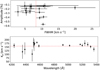 |
Fig. 11 Same as Fig. 6, but for KELT-20b. |
| In the text | |
|
Fig. 12 Same as Fig. 7, but for KELT-20b. In the upper panel, the green points represent the measurement obtained by Casasayas-Barris et al. (2019). In the middle panel, we plot several literature systemic velocities with gray horizontal lines: −23.3 ± 0.3 km s−1 (Lund et al. 2017), -21.3 ± 0.4 (Talens et al. 2018), −22.06 ± 0.35 km s−1 (Nugroho et al. 2020b), −24.48 ± 0.04 km s−1 (Rainer et al. 2021), and −26.78 ± 0.71 km s−1 (Gaia). The red horizontal line indicates the mean vsys value of −24.52 km s−1 derived in this work. |
| In the text | |
|
Fig. 13 Best-fitting νmic and νmic values obtained for each of the Fe II lines detected in the atmosphere of KELT-9b. |
| In the text | |
|
Fig. 14 Same as Fig. 13, but for KELT-20b. The values for which both νmic and νmac are consistent with 0 km s−1 or could not be determined are plotted with grey color. |
| In the text | |
|
Fig. 15 Transmission spectra of the Fe II lines at λ4522 Å, λ4583 Å, λ5018 Å, and λ5169 Å for KELT-9b (left column) and KELT-20b (right column) in comparison to the LTE (blue) and NLTE (green) synthetic profiles computed for the best fitting νmic and νmac values. The red line is the best Gaussian fit of the planetary signal. |
| In the text | |
|
Fig. 16 Synthetic transmission spectra computed considering only Fe II for KELT-9b (top panel) and KELT-20b (bottom panel). The black lines are for models created with PetitRadTrans considering all lines, while the purple lines are for models computed considering only the lines detected through the single-line analysis. |
| In the text | |
|
Fig. 17 Cross-correlation results for KELT-9b (top panels) and KELT-20b (bottom panels) using all Fe II lines. Left column: cross-correlation residual maps, where the lbright tilted signal is the RM effect, the dark signal is the Fe II atmospheric signal, the red horizontal dashed lines indicate the T1 and T4, and the dashed tilted line represents the expected velocity of the planet where for visualization reasons we assumed vsys equal to the average vsys from the single line analysis. Center-left column: same as the maps in the first column, but after correcting for the RM effect. Center-right column: Kp maps in the range of Kp from 0 to 300 km s−1, where the two horizontal gray dashed lines indicate the theoretical Kp and the best Kp values, respectively, and the vertical gray dashed line indicates the mean vsys value from the single line analysis. Right column: S/N for the best Kp value (black line), fitted Gaussian function (red dashed line), S/N obtained using only the lines detected in the single-line analysis (green line), and S/N obtained using only the lines not detected in the single-line analysis (blue line). The black dashed vertical line indicates the mean vsys value and the red vertical line indicates the velocity of the signal from the Gaussian fit. |
| In the text | |
|
Fig. 18 Rλ and Reff of the Fe II lines detected in atmosphere of KELT- 9b. Top panel : fitted Rλ for each of the lines. The dashed horizontal line indicates Rλ = RP. Bottom panel : calculated Reff values using the amplitude of the detected signal for each of the lines (black dots) and the values obtained by D’Arpa et al. (2024) (green dots). |
| In the text | |
|
Fig. 19 Same as Fig. 18, but for KELT-20b. The green dots in the top panel represent the measurements obtained by Casasayas-Barris et al. (2019) through fitting the strength of the RM effect. |
| In the text | |
Current usage metrics show cumulative count of Article Views (full-text article views including HTML views, PDF and ePub downloads, according to the available data) and Abstracts Views on Vision4Press platform.
Data correspond to usage on the plateform after 2015. The current usage metrics is available 48-96 hours after online publication and is updated daily on week days.
Initial download of the metrics may take a while.