| Issue |
A&A
Volume 676, August 2023
|
|
|---|---|---|
| Article Number | A99 | |
| Number of page(s) | 21 | |
| Section | Planets and planetary systems | |
| DOI | https://doi.org/10.1051/0004-6361/202346787 | |
| Published online | 17 August 2023 | |
The GAPS programme at TNG
XLV. HI Balmer lines transmission spectroscopy and NLTE atmospheric modelling of the ultra-hot Jupiter KELT-20b/MASCARA-2b
1
Space Research Institute, Austrian Academy of Sciences,
Schmiedlstrasse 6,
8042
Graz, Austria
e-mail: This email address is being protected from spambots. You need JavaScript enabled to view it.
2
DISAT, Università degli Studi dell’Insubria,
via Valleggio 11,
22100
Como, Italy
3
INAF - Osservatorio Astronomico di Brera,
via E. Bianchi 46,
23807
Merate, Italy
4
Dipartimento di Fisica, Università degli Studi di Torino,
via Pietro Giuria 1,
10125,
Torino, Italy
5
Institute of Physics, University of Graz,
Universitätsplatz 5,
8010
Graz, Austria
6
Instituto de Astrofísica de Andalucía (CSIC),
Glorieta de la Astronomia s/n,
18008
Granada, Spain
7
INAF - Osservatorio Astrofisico di Torino,
Via Osservatorio 20,
10025
Pino Torinese, Italy
8
Lunar and Planetary Laboratory, University of Arizona,
1629 East University Boulevard,
Tucson, AZ
85721-0092, USA
9
INAF - Osservatorio Astrofisico di Catania,
Via S. Sofia 78,
95123
Catania, Italy
10
INAF - Osservatorio Astronomico di Padova,
Vicolo dell’Osservatorio 5,
35122
Padova, Italy
11
Department of Physics, University of Oxford,
Denys Wilkinson Building, Keble Road,
Oxford,
OX1 3RH, UK
12
INAF - Osservatorio Astronomico di Cagliari,
Via della Scienza 5,
09047
Selargius (CA), Italy
13
INAF - Osservatorio Astronomico di Trieste,
via Tiepolo 11,
34143
Trieste, Italy
14
Instituto de Astrofisica de Canarias (IAC),
38205
La Laguna, Tenerife, Spain
15
Fundación Galileo Galilei - INAF,
Rambla José Ana Fernandez Pérez 7,
38712
Breña Baja, TF, Spain
16
Dipartimento di Fisica e Astronomia “Galileo Galilei” - Università di Padova,
Vicolo dell’Osservatorio 3,
35122
Padova, Italy
17
Department of Physics, University of Rome Tor Vergata,
Via della Ricerca Scientifica 1,
00133
Roma, Italy
18
Max Planck Institute for Astronomy,
Königstuhl 17,
69117
Heidelberg, Germany
19
INAF - Osservatorio Astrofisico di Arcetri,
Largo Enrico Fermi 5,
50125
Firenze, Italy
20
INFN, Sezione di Milano-Bicocca,
Piazza della Scienza 3,
20126
Milano, Italy
Received:
2
May
2023
Accepted:
28
June
2023
Abstract
Aims. We aim to extract the transmission spectrum of the HI Balmer lines of the ultra-hot Jupiter (UHJ) KELT-20b/MASCARA-2b from observations and to further compare the results with what was obtained through forward modelling, accounting for non-local thermodynamic equilibrium (NLTE) effects.
Methods. We extracted the line profiles from six transits obtained with the HARPS-N high-resolution spectrograph attached to the Telescopio Nazionale Galileo telescope. We computed the temperature-pressure (TP) profile employing the HELIOS code in the lower atmosphere and the CLOUDY NLTE code in the middle and upper atmosphere. We further used CLOUDY to compute the theoretical planetary transmission spectrum in LTE and NLTE for comparison with observations.
Results. We detected the Hα (0.79±0.03%; 1.25 Rp), Ηβ (0.52±0.03%; 1.17 Rp), and Ηγ (0.39±0.06%; 1.13 Rp) lines, and we detected the Ηδ line at almost 4σ (0.27±0.07%; 1.09 Rp). The models predict an isothermal temperature of ≈2200 K at pressures >10−2 bar and of ≈7700 K at pressures <10−8 bar, with a roughly linear temperature rise in between. In the middle and upper atmosphere, the NLTE TP profile is up to ~3000 K hotter than in LTE. The synthetic transmission spectrum derived from the NLTE TP profile is in good agreement with the observed HI Balmer line profiles, validating our obtained atmospheric structure. Instead, the synthetic transmission spectrum derived from the LTE TP profile leads to significantly weaker absorption compared to the observations.
Conclusions. Metals appear to be the primary agents leading to the temperature inversion in UHJs, and the impact of NLTE effects on them increases the magnitude of the inversion. We find that the impact of NLTE effects on the TP profile of KELT-20b/MASCARA-2b is larger than for the hotter UHJ KELT-9b, and thus NLTE effects might also be relevant for planets cooler than KELT-20b/MASCARA-2b.
Key words: planets and satellites: atmospheres / planets and satellites: individual: KELT-20b / planets and satellites: individual: MASCARA-2b
© The Authors 2023
 Open Access article, published by EDP Sciences, under the terms of the Creative Commons Attribution License (https://creativecommons.org/licenses/by/4.0), which permits unrestricted use, distribution, and reproduction in any medium, provided the original work is properly cited.
This article is published in open access under the Subscribe to Open model. This email address is being protected from spambots. You need JavaScript enabled to view it. to support open access publication.
1 Introduction
Transmission and emission spectroscopy, both from the ground and from space, have led to significant advances in our understanding of exoplanetary atmospheres. In this context, ultra-hot Jupiters (UHJs), that is, planets with an equilibrium temperature (Teq) greater than ≈2000 K and for which H− opacity and thermal dissociation are significant, play a key role. This is because the high atmospheric temperatures of these planets lead to large pressure scale heights and, thus, more easily detectable spectral features. Furthermore, these planets are typically detected orbiting rather bright intermediate-mass stars (i.e. F- and A-type), which facilitates high-quality observations, particularly at optical wavelengths.
With an equilibrium temperature of nearly 4000 K, KELT-9b (Gaudi et al. 2017) is the most extreme of the UHJs and so far also the most studied, both observationally and theoretically. Because of the brightness of the host star (V ≈ 7.6 mag), KELT-20b (Lund et al. 2017), also known as MASCARA-2b (Talens et al. 2018), is one of the most studied UHJs in terms of atmospheric characterisation observations, mainly through ground-based high-resolution spectroscopy.
KELT-20b/MASCARA-2b orbits its A2V host star (HD 185603) with a period of about 3.47 days, which implies an equilibrium temperature of about 2200 K, assuming zero albedo and complete heat redistribution (Lund et al. 2017). Photometric transit observations provide a rather precise measurement of the planetary radius of about 1.83 RJ (Talens et al. 2018), but the broad spectral lines due to the rapid rotation of the host star (ν sin i = 116.23 km s−1; Prot = 0.695 days; Rainer et al. 2021) hinder a precise measurement of the planetary mass, for which just a 3σ upper limit of 3.51 MJ has been obtained (Lund et al. 2017).
Multiple ground-based transmission spectroscopy observations enabled the clear detection of the Hα and Hβ hydrogen Balmer lines, as well as of the NaI D doublet, the CaII infrared triplet, the CaII H&K lines, and multiple FeII lines (Casasayas-Barris et al. 2018, 2019; Nugroho et al. 2020). The cross-correlation technique led to the further detection of FeI, MgI, and CrII in the planetary atmosphere, as well as to the confirmation of some of the previously detected species (Stangret et al. 2020; Hoeijmakers et al. 2020; Nugroho et al. 2020; Rainer et al. 2021; Cont et al. 2022; Bello-Arufe et al. 2022; Johnson et al. 2023).
Thanks to its high equilibrium temperature, KELT-20b/MASCARA-2b has also been observed during and around secondary eclipse both from the ground and from space. Applications of the cross-correlation technique to high-resolution ground-based day-side observations enabled the detection of FeI, FeII, SiI, and CrI on the atmospheric day side (Borsa et al. 2022; Cont et al. 2022; Johnson et al. 2023; Yan et al. 2022; Kasper et al. 2023). Space-based secondary eclipse observations led to the detection of water in the lower atmosphere, the measurement of the brightness temperature in different bands, and constraints on the atmospheric metallicity (Fu et al. 2022). These observations have also been used to constrain the atmospheric temperature-pressure (TP) profile at pressures higher than 10−5 bar, which is probed by the cores of metal lines in the optical band (Borsa et al. 2022; Fu et al. 2022; Yan et al. 2022). The detection of emission features close to the secondary eclipse clearly indicates the presence of a temperature inversion, that is, an atmospheric temperature increasing with decreasing pressure. Retrievals of the TP profile performed on the observations confirm the temperature increase at the ~0.1 bar level and a rather isothermal profile of about 2200 K at higher pressures, which is supported by forward modelling (Borsa et al. 2022; Fu et al. 2022; Yan et al. 2022).
Several previous studies sought to identify the radiatively active species that, in addition to what provided by hydrogen Balmer line heating (García Muñoz & Schneider 2019), contribute to the temperature inversion, focusing particularly on the search for molecules such as TiO, VO, and FeH. These attempts have not been successful (Nugroho et al. 2020; Johnson et al. 2023), the only exception being that FeH was tentatively detected by Kesseli et al. (2020), though this was not confirmed in follow-up observations (Johnson et al. 2023). These non-detections and the simultaneous detection of a number of neutral and singly ionised atomic species support the idea that metal absorption of the stellar radiation, particularly of ultraviolet (UV) photons, is at the origin of the temperature inversion, as predicted by models of UHJs (Lothringer et al. 2018; Lothringer & Barman 2019; Fossati et al. 2021). This was particularly evident in the case of KELT-9b, for which a broad range of atomic species has been detected (e.g. Hoeijmakers et al. 2018, 2019; Yan et al. 2019; Turner et al. 2020; Borsa et al. 2021b; Pino et al. 2020). Furthermore, for KELT-9b, Fossati et al. (2021) show that non-local thermodynamic equilibrium (NLTE) effects lead to a significant overpopulation of FeII and underpopulation of MgII, which are the key agents driving heating and cooling, respectively, in the planetary atmosphere. In particular, the NLTE-driven overpopulation of excited FeII significantly increases the absorption of stellar near-UV radiation, further increasing the heating rate. This stems from the fact that the near-UV spectral range, which is also where the host star’s spectral energy distribution peaks, contains several FeII lines that rise from low energy levels. This conclusion is supported by the fact that the forward model presented by Fossati et al. (2021), which accounts for NLTE effects, was able not only to fit the observed hydrogen Balmer line profiles, but also to predict the presence of the OI infrared triplet and its strength in the planetary transmission spectrum, which was then confirmed by observations (Borsa et al. 2021b).
Here, we present the results of transmission spectroscopy of KELT-20b/MASCARA-2b based on six transit observations conducted with the aim of detecting hydrogen Balmer line absorption and constraining the shape of the absorption line profiles. This work follows the observations of Rainer et al. (2021) and Borsa et al. (2022) of this same planet; they respectively focused on measuring the Rossiter-McLaughlin (RM) effect during transit and detecting species through day-side measurements. We interpret the hydrogen Balmer line observations by using a forward model that spans from the lower atmosphere (10 bar) to the upper atmosphere (~10−12 bar) and includes NLTE effects, comparable to the model used by Fossati et al. (2021) to explain the observations of KELT-9b.
This paper is organised as follows. Section 2 presents the observations and the methodology employed to analyse the data. Section 3 describes the atmospheric modelling. Section 4 presents the modelling results (Sect. 4.1) and the hydrogen Balmer line profiles obtained from the observations (Sect. 4.2). In Sect. 5 we compare the observational and modelling results, present the synthetic UV-to-infrared transmission spectrum, and extract more information about the properties of the planetary atmosphere. Finally, we present our conclusions in Sect. 6.
2 Observations and data analysis
KELT-20b/MASCARA-2b was observed in the optical band with the high resolution (R ~ 115 000) HARPS-N spectrograph (Cosentino et al. 2012) located at Telescopio Nazionale Galileo (TNG) during six different transits between the years 2017 and 2022. The first three transits that we analyse are taken from the TNG archive and have previously been analysed by Casasayas-Barris et al. (2019), who looked for the hydrogen Balmer lines in the planetary atmosphere, as well as for other chemical species. We add here further three transits taken in the context of the atmospheric characterisation part of the GAPS programme (e.g. Borsa et al. 2019; Giacobbe et al. 2021; Guilluy et al. 2022), for which the H Balmer lines were not analysed before.
Table 1 summarises the observations considered in this work. Nights 2 and 6 present an unstable signal-to-noise ratio (S/N). Therefore, for these nights we decided to discard all spectra with S/N < 50. Furthermore, nights 2 and 3 suffered a problem that affected the telescope’s Atmospheric Dispersion Corrector (ADC; see Casasayas-Barris et al. 2019, for more details), which causes wavelength-dependent flux losses in particular in the blue part of the spectrum, and thus called for particular attention in the normalisation process. All spectra have been reduced with the standard data reduction software (DRS) v3.7 and we analysed the one-dimensional pipeline products (i.e. s1d), which cover the 3800–6900 Å wavelength range and have a constant wavelength step of 0.01 Å.
We focused our attention on the Balmer lines Hα, Hβ, Hλ, and Hδ. For each transit, we calculated the transmission spectra following a procedure similar to that described by Wyttenbach et al. (2015). We started by correcting telluric lines across the whole wavelength range, employing MOLECFIT v4.2.3 (Smette et al. 2015; Kausch et al. 2015) and following the prescriptions of Allart et al. (2017). In particular, we corrected for absorption caused by telluric O2 and H2O. An example of the correction performed is presented in Fig. 1. We then Doppler-shifted all spectra in the stellar reference frame by subtracting the theoretical stellar radial velocity at each orbital phase, and normalised them to the same continuum level in a narrow range around each considered line (i.e. Hα 6525–6595 Å; Hβ 4810–1910 Å; Ηγ 4310–1370 Å; and Ηδ 4080–4120 Å). We then calculated an average out-of-transit spectrum (master-out, Mout) employing a weighted average on the stellar flux, divided each spectrum by Mout, and normalised again to remove any remaining small linear trend that has propagated throughout the analysis procedure. This last step was particularly important for the analysis of nights 2 and 3, because of the faulty ADC affecting the continuum flux.
At this point, we corrected the residual spectra for the contamination given by stellar rotation (i.e. the RM effect) and centre-to-limb variations (CLVs), which are known to possibly affect the transmission spectrum and eventually cause false detections (e.g. Borsa & Zannoni 2018; Casasayas-Barris et al. 2020). To this end, we created a model of the contamination as in Borsa et al. (2021a), which follows the approach of Yan et al. (2017), by inserting ATLAS9 stellar atmosphere models and a VALD line list (Ryabchikova et al. 2015) into Spectroscopy Made Easy (SME; Piskunov & Valenti 2017), based on the system parameters listed in Table 2. The modelled contamination has been calculated for each observed orbital phase and removed from the data by dividing for it. The extension of the planetary radius Rp,λ used to model the CLV and RM effects on each of the Balmer lines has been calculated iteratively, until reaching a value for which the final amplitude of the Gaussian fit to the line in the transmission spectrum (see Sect. 4.2) and the value of Rp,λ used in the CLV+RM model coincide within 0.5σ, with σ being the error-bar on the line depth calculated as described in Sect. 4.2.
We then calculated the final transmission spectrum for each night by shifting all residual spectra in the planetary reference frame and performing a weighted average of all residual spectra taken during the full part of the transit (i.e. between the second and third contact points). We finally obtained the average transmission spectrum of each Balmer line by performing a weighted average of the transmission spectra obtained from each of the six nights of observation.
Log of the transit observations of KELT-20b/MASCARA-2b used in this work.
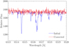 |
Fig. 1 Example of MOLECFIT tellurics correction in the proximity of the Hα line. |
Adopted parameters of the KELT-20/MASCARA-2 system.
3 Atmospheric modelling
We computed the theoretical atmospheric TP profile of KELT-20b/MASCARA-2b at the sub-stellar point, employing the scheme described in detail by Fossati et al. (2021). It consists of the separate computation of TP profiles of the lower (P ≳ 10−4 bar) atmosphere with the HELIOS code (Malik et al. 2017, 2019) and of the upper (P ≲ 10−4 bar) atmosphere with the CLOUDY NLTE radiative transfer code (Ferland et al. 2017), the latter through the CLOUDY for Exoplanets (CfE) interface (Fossati et al. 2021). The HELIOS and CLOUDY TP profiles are then joined together to obtain a single TP profile that is used as starting point to derive the atmospheric chemical composition and transmission spectra. We adopt this scheme, because HELIOS does not account for NLTE effects that are relevant in the middle and upper atmosphere, while CLOUDY, which considers NLTE effects, is unreliable in the lower atmosphere at densities greater than 1015 cm−3 (see Ferland et al. 2017 and Fossati et al. 2021 for more details).
HELIOS1 is a radiative-convective equilibrium code taking as input planetary mass, radius, and atmospheric abundances, orbital semi-major axis, and stellar radius and effective temperature, further assuming equilibrium abundances, which we computed using the FASTCHEM2 code (Stock et al. 2018). For the simulation, we divided the atmosphere into 100 layers logarithmically distributed in the 100−10−9 bar pressure range. We computed the HELIOS model with a heat redistribution parameter, f, which accounts for the day-to-night side heat redistribution efficiency, equal to 0.25. This leads to a TP profile in the lower atmosphere comparable to that obtained from retrievals of day-side observations (Borsa et al. 2022; Fu et al. 2022). Given the high planetary atmospheric temperature, we considered additional opacities not present in the public version of the HELIOS code as described by Fossati et al. (2021).
CLOUDY is a general-purpose plane-parallel microphysics radiative transfer code that accounts for (photo)chemistry and NLTE effects (Ferland et al. 1998, 2013, 2017). For the calculations presented here, we employed CLOUDY version 17.03. CLOUDY computations include a wide range of atomic (i.e. all elements up to Zn) and molecular species, and are valid across a wide interval of plasma temperatures (3–1010 K) and densities (<1015 cm−3). This covers the parameter space of what is expected in upper planetary atmospheres. CLOUDY is a hydrostatic code and we come back to the validity of this assumption in the case of KELT-20b/MASCARA-2b in Sect. 5. Details of the code relevant to exoplanet atmospheric calculations are given in Sect. 2.2.1 of Fossati et al. (2021).
To set up the CLOUDY runs, we employed the CfE interface, which writes CLOUDY input files on the basis of input parameters given by the user, runs CLOUDY, and reads CLOUDY output files. Then, CfE uses the information contained in the output files to set up a new CLOUDY calculation in an iterative process until the temperature profile has converged. The details of how CfE sets up CLOUDY input files and the iteration procedure are described in Sect. 2.2.2 of Fossati et al. (2021).
For the atmospheric modelling, we considered the system parameters listed in Table 2. For the calculations, we employed a synthetic spectral energy distribution computed with the PHOENIX code3 (Husser et al. 2013). Because the host star is earlier than spectral type A3–A4, we did not add any X-ray and extreme ultraviolet (EUV) emission to the photospheric fluxes provided by the PHOENIX model (Fossati et al. 2018). However, rapidly rotating early-type stars could present magnetic activity close to the equator as a result of the low local effective temperature caused by gravity darkening, but this is not the case for KELT-20/MASCARA-2, because its rotational velocity is just about 45% of the critical break-up velocity. This further justifies our assumption of considering just photospheric emission.
The 1015 cm−3 density limit above which CLOUDY’s computation of the heating and cooling rates becomes unreliable lies at a pressure of about 0.3 mbar, while the continuum lies at a pressure of about 6 mbar. This is the pressure at which the HELIOS model gives an optical depth of 2/3 around 5000 Å, which is the wavelength corresponding to the peak efficiency of the MASCARA optical system used to discover the planet (Talens et al. 2017). For this reason, we run CfE setting the planetary transit radius of 1.83 RJ (Talens et al. 2018) at the reference pressure (p0) of 6 mbar. The top panel of Fig. A.1 shows a comparison between CLOUDY TP profiles obtained setting the planetary transit radius at different p0 values of 100, 6, and 1 mbar, indicating that uncertainties on the location of the reference pressure do not impact the results. To save on computational time, for the CLOUDY calculations we considered all elements up to Zn and only hydrogen molecules (i.e. H2,  ,
,  ), because the inclusion of all molecules present in the CLOUDY database did not affect the resulting TP profile (see the middle panel of Fig. A.1). Finally, in agreement with Fossati et al. (2021), we find that the number of layers considered for the computation of the TP profile (i.e. 180) does not impact the results (see the bottom panel of Fig. A.1).
To mimic atmospheric heat redistribution in the computation of the CLOUDY TP profiles, we scaled the spectral energy distribution multiplying it by a factor f1 ≤ 1. Following Fossati et al. (2021), we computed TP profiles with varying f1 values looking for the one leading to the TP profile that best matches the HELIOS one around the 10−4 bar level. We finally adopted f1 = 1.0, but we remark that the value employed for f1 has no significant impact on the TP profile at pressures lower than about 10−5 bar (Fossati et al. 2021). For all calculations, we assumed solar atmospheric composition (Lodders 2003).
4 Results
4.1 Atmospheric TP and abundance profiles
We resampled the final theoretical TP profile, obtained by joining the HELIOS and CLOUDY profiles, over 200 layers equally spaced in log p ranging from 10 bar to 4×10⁻¹² bar. The considered pressure range is wide enough to cover the formation region of UV, optical, and infrared lines in the transmission spectrum.
We combined the HELIOS and CLOUDY theoretical TP profiles at a pressure of 10−4 bar and then fitted the entire profile with a polynomial to smooth the edge at the joining point, further interpolating on the final pressure scale. Figure 2 shows the composite theoretical TP profile in comparison to the original HELIOS and CLOUDY theoretical profiles. The final profile is roughly isothermal at pressures higher than about 10 mbar and lower than about 10−8 bar, while the section in between those pressures is characterised by a linear temperature rise from about 2200 K up to about 7700 K. Therefore, the temperature varies by about 5500 K from the lower to the upper atmosphere, which implies that an isothermal approximation for the entire atmosphere would be inappropriate for this planet.
We identified the Hα line formation region by computing CLOUDY models starting from the top of the atmosphere (at 10−12 bar) and subsequently increasing the pressure of the lower considered layer, further looking at the transmitted spectrum around the Hα line. The top boundary of the line formation region (i.e. at low pressure) was then set where, with increasing pressure of the lower considered layer, the transmitted spectrum started to show Hα absorption, while the bottom boundary of the line formation region (i.e. at high pressure) was set where the Hα absorption stopped increasing with increasing pressure of the lower considered layer. In this way, we obtained that the Hα line formation region is confined in a rather narrow pressure range between about 10−10 and 10−7 bar, where the temperature is higher than about 7000 K. This range is similar to that found for KELT-9b using the same modelling scheme employed here (Turner et al. 2019; Fossati et al. 2021). Both host stars (i.e. KELT-9 and KELT-20/MASCARA-2) are not supposed to have a chromosphere (Fossati et al. 2018), and thus their Lyα lines are totally absorbed, which prevents hydrogen photo-excitation. Therefore, the excitation of the hydrogen atoms to the n = 2 level, which then leads to the formation of the Balmer lines, has to occur mostly thermally. This is further confirmed by the fact that photoionisation and subsequent recombination to the n = 2 level have a low probability in comparison to thermal excitation, because of the very low EUV emission of the host star.
The derived temperature inversion supports the results of secondary eclipse observations (Borsa et al. 2022; Fu et al. 2022; Yan et al. 2022) as well as previous general atmospheric modelling of UHJs (Lothringer et al. 2018), though the inclusion of NLTE effects strongly increases the magnitude of the inversion compared to previous local thermodynamic equilibrium (LTE) modelling. The retrieval approach followed by Borsa et al. (2022) and Yan et al. (2022) to constrain the TP profile from their secondary eclipse observations assumes a two-point TP profile where the temperature below the higher pressure point and above the lower pressure point was considered to be isothermal, with a linear gradient in between. At the two nodes of the two-point TP profile, they obtained a lower temperature value lying around 2200 K with the turning point located in the 0.1–1 bar range and a higher temperature value of about 5300 K with the turning point at a pressure of about 10−5 bar. Instead, Fu et al. (2022) did not make any assumption on the shape of the TP profile obtaining an isothermal profile at ≈2200 K at pressures higher than about 10−2 bar, with a roughly linearly decreasing temperature at lower pressures up to 10−4 bar, where they stopped their calculation. The assumed two-point shape of the TP profile resembles well the temperature profile obtained by combining HELIOS and CLOUDY. As expected by the choice of parameters used to compute the HELIOS TP profile, in the lower atmosphere (>10−5 bar) the retrieved profiles match ours well (i.e. within 1σ). Instead, in the upper atmosphere (<10−5 bar) the retrieved temperatures are more than 1500 K cooler and the turning points located at a 1000 times higher pressure compared to what is predicted by CLOUDY (see Fig. A.2). This difference can be ascribed to the fact that emission observations do not probe high enough in the atmosphere to cover the pressures below 10−5 bar (Borsa et al. 2022; Fu et al. 2022; Yan et al. 2022).
To obtain a homogeneous synthetic chemical atmospheric structure, we passed the composite TP profile to CLOUDY (see Fossati et al. 2021, for more details). Figure 3 shows the theoretical density profiles with respect to the total hydrogen density of the main hydrogen-bearing species (neutral hydrogen HI, protons HII, Η−, molecular hydrogen H2,  ,
,  ), plus electrons (e−). The middle and upper atmosphere (<10−3 bar) are largely dominated by neutral hydrogen, which is significantly ionised only at the very top, around 5×10⁻¹¹ bar, namely a thousand times lower pressure than what the same model predicted for KELT-9b (Fossati et al. 2021). This is ultimately caused by the fact that KELT-9b is more irradiated by EUV photons as a result of the hotter host star (both stars have only photospheric emission; Fossati et al. 2018) and closer orbital separation. Instead, the lower atmosphere is dominated by H2 and neutral hydrogen, with H2 rapidly decreasing with decreasing pressure below the 10 mbar level. As expected given that KELT-20b/MASCARA-2b is an UHJ (e.g. Arcangeli et al. 2018), H− is relatively abundant with its density first increasing with decreasing pressure up to the 1 μbar level and then decreasing at lower pressures.
Figure 4 shows the theoretical mixing ratio as a function of pressure for some of the most relevant elements in terms of abundance and observability. As a consequence of the assumption of solar composition, helium is the second most abundant element throughout. Thanks to its high ionisation energy, oxygen remains in its neutral state almost up to the top of the considered pressure range (similarly to hydrogen), while carbon, which has a slightly lower ionisation energy, starts to ionise significantly at the 1 nbar level. Sodium and potassium have similar ionisation energies and indeed behave similarly, with the ionisation occurring in the 0.01–1 bar pressure range. Also, as a result of their similar ionisation energies, magnesium, silicon, and iron have comparable behaviours with the singly ionised atoms becoming dominant at the millibar level. This result confirms that FeI and FeII lines are likely to form at different altitudes in the planetary atmosphere, as suggested by the different velocities and widths of these features detected through the cross-correlation technique (Stangret et al. 2020; Nugroho et al. 2020; Hoeijmakers et al. 2020). Among those shown in Fig. 4, calcium is the only element for which the second ionised species become dominant within the simulated pressure range.
Figure 2 shows that in the upper atmosphere the CLOUDY TP profile is about 3000 K hotter than predicted by the HELIOS model. Remarkably, this difference is about 1000 K larger than that found for KELT-9b. Following Fossati et al. (2021), we tested whether this difference could be ascribed to NLTE effects by computing an additional TP profile with CLOUDY, but assuming LTE. We remark that even when enforcing the LTE assumption, CLOUDY computes the populations of the first two energy levels of hydrogen in NLTE. In the middle and upper atmosphere, the CLOUDY LTE TP profile, shown in Fig. 2, is significantly cooler than the NLTE one and lies close to that computed with HELIOS. Furthermore, the similarity between the CLOUDY LTE and HELIOS TP profiles in the middle atmosphere suggests that molecules do not have a significant impact on the shape of the TP profile at pressures lower than 0.1 mbar.
To identify the elements primarily responsible for the difference between the LTE and NLTE TP profiles, we computed CLOUDY NLTE TP profiles excluding one of the elements at a time, except for H and He that we always kept in each model. Similarly to the case of KELT-9b, we found that Fe and Mg are the elements that most shape the TP profile. In particular, Fe dominates the heating and Mg the cooling in the middle and upper atmosphere (Fig. 5). Removing Fe leads to a TP profile that in the middle and upper atmosphere is between 1000 and 2000 K cooler than that obtained including Fe. Instead, excluding Mg leads to an about 300 K hotter TP profile. The other elements, instead, contribute less than 50 K to the heating or cooling in the planetary atmosphere.
Compared to the case of KELT-9b (see Fig. 7 of Fossati et al. 2021), the TP profile computed excluding Fe shows a significantly smaller temperature increase in the upper atmosphere (<10−10 bar), which is most likely due to the weaker EUV emission of KELT-20/MASCARA-2 compared to KELT-9. This suggests that metals are primarily responsible for the heating and cooling in the middle and upper atmosphere. To confirm this, we extracted from the CLOUDY run the three main heating and cooling agents and display them in Fig. 6. We find that metal line absorption (particularly of Fe; Fig. 5) is the main heating mechanism throughout the entire middle and upper atmosphere, with photoionisation playing a secondary role, while numerous species contribute to the cooling of the middle and upper atmosphere, but Mg is by far the most important atmospheric coolant.
To deepen our understanding of the roles played by Mg and Fe in shaping the TP profile, we took the output obtained after the last NLTE CfE iteration and used it as input for a further CLOUDY run, but considering only FeI (i.e. FeI is not allowed to ionise) or FeII (i.e. FeII is not allowed to ionise or recombine), fixing the FeI or FeII density profile to that obtained accounting for all elements and ions, and then did the same with Mg as well. Figure 7 shows the temperature and the total heating rate as a function of pressure obtained in all these cases and it clearly indicates that most of the heating is caused by FeII, while most of the cooling is caused by MgII. Therefore, the combined impact of NLTE effects on the level populations of Fe and Mg (see Figs. A.3–A.6) leads to a general temperature increase in the middle and upper atmosphere when compared to the LTE profile.
Interestingly, in the case of KELT-20b/MASCARA-2b, the inclusion of NLTE effects leads to a larger temperature increase in the middle and upper atmosphere compared to KELT-9b, although the latter is hotter and orbits a hotter star. This can be understood by looking at the departure coefficients that are defined as
 (1)
(1)
where nNLTE and nLTE are the densities of a given atom lying in a certain level in NLTE and LTE, respectively, with the nLTE profiles obtained through the Boltzmann equation. A comparison of the Mg and Fe departure coefficients computed by CLOUDY for the two planets in the middle and upper atmosphere (see Figs. A.3 to A.6 for KELT-20b/MASCARA-2b and Figs. C.1 to C.5 of Fossati et al. 2021) indicates that the b profiles obtained for FeI and Mg for KELT-20b/MASCARA-2b are on average significantly smaller (larger in modulus) than those obtained for KELT-9b. Therefore, the middle and upper atmosphere of KELT-20b/MASCARA-2b has less MgII available for driving the cooling, and thus the larger difference between the LTE and NLTE TP profiles obtained for KELT-20b/MASCARA-2b compared to KELT-9b might be ascribed to a lack of cooling rather than to an increase in heating.
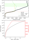 |
Fig. 2 Theoretical atmospheric structure obtained for KELT-20b/MASCARA-2b. Top: HELIOS (dashed orange line) and CLOUDY (in NLTE; dashed cyan line) TP profiles. The solid black line shows the composite TP profile. The horizontal dotted black line indicates the location of the continuum according to the HELIOS model. The horizontal dash-dotted red line gives the location of the CLOUDY’s upper-density limit of 1015 cm−3. The dashed dark green line shows the CLOUDY TP profile computed assuming LTE. The hatched area indicates the Hα line formation region. Bottom: pressure (black; left y-axis) and temperature (red; right y-axis) composite theoretical profiles as a function of the planetary polar radius. |
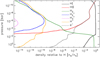 |
Fig. 3 Density relative to the total density of hydrogen for neutral hydrogen (HI; solid black line), protons (HII~; red), molecular hydrogen (H2; dark green), |


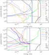 |
Fig. 4 Atmospheric mixing ratios obtained for metals. Top: mixing ratios for hydrogen (solid black line), H2 (dotted black), He (red), C (blue), O (dark green), Na (violet), K (orange), and electrons (bright green) as a function of atmospheric pressure. Neutral (XI), singly ionised (XII), and doubly ionised (XIII) species are shown as solid, dashed, and dash-dotted lines, respectively. Bottom: same as the top panel, but for Mg (red), Si (blue), Ca (dark green), and Fe (violet). The hydrogen, H2, and e− mixing ratios are shown in both panels for reference. |
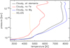 |
Fig. 5 Comparison between the NLTE CLOUDY TP profiles obtained considering all elements up to Zn (solid black line) and excluding Fe (solid red line) or Mg (solid blue line). The dashed orange line shows the HELIOS (i.e. LTE) TP profile for reference. |
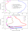 |
Fig. 6 Heating and cooling contributions in the atmosphere of KELT-20b/MASCARA-2b. Top: contribution to the total heating as a function of pressure. At each pressure bin, the plot shows the three most important heating processes. The main heating processes occurring in the middle and upper atmosphere are hydrogen photoionisation (red; photoionisation of HI lying in the ground state), metal line absorption (blue), H− absorption (green), photoionisation of hydrogenic species (photoionisation of excited HI; magenta), and collisions with H2 (brown). Bottom: contribution to the total cooling as a function of pressure. At each pressure bin, the plot shows the three most important cooling agents. |
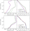 |
Fig. 7 Atmospheric structure and heating rate obtained from isolating the impacts of Fe and Mg ions. Top: temperature (left) and total heating rate (right) as a function of pressure obtained accounting for all elements (black; same as in Figs. 2 and 5), considering that in the planetary atmosphere Fe exists only in the form of FeI (blue), only in the form of FeII (green), or is absent (i.e. no Fe; same as Fig. 5; red). Bottom: same as the top, but for Mg. |
4.2 Hydrogen Balmer lines
We detect Hα, Hβ and Ηγ with an absorption depth of 0.789±0.034% (≈23σ), 0.517±0.034% (≈15σ), and 0.394±0.057 % (≈7σ), respectively. We also report the detection of Ηδ at almost 4σ with an absorption depth of 0.272±0.070 %. We note that KELT-20b/MASCARA-2b is only the second planet, after KELT-9b, for which Ηδ has been detected (Wyttenbach et al. 2020). The obtained line depths translate into planetary radii of about 1.25 Rp, 1.17 Rp, 1.13 Rp, and 1.09 Rp for Hα, Hβ, Ηγ, and Ηδ, respectively, under the assumption of a symmetrically distributed atmosphere. The line profiles obtained from the HARPS-N observations are shown in Fig. 8.
The Hα, Hβ and marginally Ηγ lines have already been identified in the atmosphere of KELT-20b/MASCARA-2b by Casasayas-Barris et al. (2019) from the analysis of the transits collected during nights 1 to 3, plus an additional transit taken with the CARMENES spectrograph. We note that in the present work we do not use the CARMENES data to avoid any possible instrumental systematics, since one more transit would not add much to our HARPS-N six-transit dataset. Our results are in agreement within 1σ with theirs (see Fig. A.7), despite the fact that Casasayas-Barris et al. (2019) optimised the radial velocity semi-amplitude of the planet Kp for each transit with a Markov chain Monte Carlo analysis, while we used the same theoretical Kp (Table 2) for all six datasets. Planetary atmospheric variations during transit could mimic Kp variations. When the part of the atmosphere in view during transit changes (because of the orbital movement and planetary rotation), regions of the atmosphere with different dynamics could become visible, which could lead to discrepancies between the actual planetary velocity and the system of velocity of the atmosphere itself. This phenomenon has been clearly observed in the case of WASP-76b (Ehrenreich et al. 2020; Kesseli & Snellen 2021). The possibility that this could happen also for KELT-20b/MASCARA-2b has been mentioned by Rainer et al. (2021), but their analysis of Fe cross-correlation functions did not lead to a statistically significant detection of this phenomenon.
Our approach of using the same Kp for all the transits is justified by the fact that we aim to obtain an average planetary line profile to compare with theoretical simulations, which do not account for any possible transit-by-transit variability. To support this approach, we looked for any variation of the Hα and Hβ absorption depths, centre, and full width half maximum (FWHM) among the six transits when using the same Kp value. The absorption depth, centre, and FWHM values were derived by performing a Gaussian fit of average transmission spectrum given by each transit with a linear regression4 using CPNest5 Del Pozzo & Veitch 2022), which is a PYTHON implementation of the nested sampling algorithm (Skilling 2006). By looking at the transmission spectra individually, we could find neither significant variations beyond the 2.1σ level nor correspondences in the pattern shown by the absorption depths, centre, and FWHM between the two lines (see Fig. 10 and Table A.1). A further check of our results has been performed independently by using the Sloppy pipeline (Sicilia et al. 2022), obtaining fully compatible results.
To further validate the use of the same Kp, we compared the depths of the Hα line with varying Kp. Within a reasonable range of Kp values (Fig. 9), the depth of the average line is compatible within error bars. This fact is a consequence that the width of the line profile is quite large, and the deviation of the average line depth value becomes significant only for Kp values ≲50 km s−1 or ≳280 km s−1.
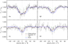 |
Fig. 8 Comparison between observed and synthetic Hα (top left), Bβ (top right), Ηγ (bottom left), and Hδ (bottom right) line profiles. The solid black line shows the observations, while to guide the eye the black dots show the observed profiles re-binned to about 4.5 km s−1. The dashed red line indicates the Gaussian fit to the observations. The solid blue and dash-dotted green lines show the CLOUDY synthetic line profiles computed in NLTE and LTE, respectively. The central wavelengths of the Balmer lines (in vacuum) used to convert the wavelengths into velocities are 6564.60 Å for Hα, 4862.71 Å for Hβ, 4341.69 Å for Ηγ, and 4102.892 Å for Hδ. |
5 Discussion
5.1 Comparison with the observations
To compare the observations with the modelling results and further explore the impact of NLTE effects, we used CLOUDY to compute synthetic transmission spectra in both LTE and NLTE. To this end, we followed the procedure described by Young et al. (2020) and Fossati et al. (2020), dividing the entire atmosphere into 100 layers equally spaced in log p and considering a spectral resolution of 100 000. The theoretical NLTE transmission spectrum was computed employing the composite TP profile shown in Fig. 2 and enabling NLTE throughout the entire transmission spectrum calculation. Instead, the theoretical LTE transmission spectrum was computed employing the LTE TP profile shown in Fig. 2, further joined together with the HELIOS profile as done to obtain the composite NLTE TP profile (see Sect. 4.1), and imposing the LTE assumption also for the CLOUDY transmission spectrum calculation.
The CLOUDY calculations presented above take the substellar point into account, but the computation of transmission spectra implies a different geometry (i.e. from emission geometry to transmission geometry), which then calls for a new calibration of the reference pressure, p0, that corresponds to the reference radius, R0, that is, the measured transit radius, Rp. To obtain a more robust calibration, particularly when comparing the model with the observations, we employed a procedure different from that followed by Fossati et al. (2021). We computed several transmission spectra by setting p0 at different pressure levels in the 0.001–0.1 bar pressure range. We then convolved each synthetic transmission spectrum with the MASCARA instrument bandpass (Talens et al. 2017) to obtain Rp/Rs as a function of p0. Finally, for the comparison with the observations, we considered the synthetic transmission spectrum computed with the p0 value, which leads to the transmission spectrum that best matches the observed Rp/Rs of 0.1175 (Talens et al. 2018). For the LTE and NLTE theoretical transmission spectra, we find best-fitting reference pressure values of 0.001 bar and 0.002 bar, respectively.
To explore the possible error introduced by an inaccurate p0–Rp calibration, Fig. A.8 shows theoretical NLTE transmission spectra in the region of the Hα line computed by setting the transit radius at the reference pressure of 0.1, 0.01, and 0.001 bar, both before and after normalisation. As expected, the non-normalised synthetic transmission spectra have different continua, with the difference decreasing with increasing p0, because the atmosphere becomes more and more compact with increasing pressure. Following normalisation to the continuum, we find that the actual choice of reference pressure value has no significant impact on the line absorption depth, particularly when compared with the noise level of the observations. Together with the top panel of Fig. A.1, this shows that the choice of reference pressure, in the computation of both the theoretical TP profile and transmission spectrum, has no significant impact on the modelling results.
Figure 8 shows the comparison between the observed and the synthetic Hα, Hβ, Ηγ, and Ηδ line profiles (for context, Fig. A.9 shows the profiles of the HI departure coefficients). As also shown by the χ2 and reduced χ2 ( ) values listed in Table 3, the NLTE synthetic spectra are a good match to the data, while the synthetic LTE line profiles are systematically weaker than the observations. This is mostly due to the difference in underlying TP profiles employed to compute the theoretical transmission spectra, particularly because, even in LTE, CLOUDY computes the hydrogen population of the first two energy levels accounting for NLTE effects (see Fossati et al. 2021).
The NLTE synthetic spectra slightly overestimate the line absorption depth compared to the observations. Furthermore, the predicted line profiles are significantly broader and rounder than the observed ones, which are instead more triangular. These differences are probably caused by the fact that we consider only the day-side temperature profile, and thus assume that the TP profile computed at the sub-stellar point is valid across the entire planet (i.e. both day and night sides). This leads us to overestimate the gas temperature at the terminator region and thus the line absorption depth and broadening, because the night side has a lower temperature. Without this assumption the lines forming on the night side of the terminator region would not be as strong and broad, and would mostly contribute to the shape of the line core, making the synthetic lines weaker and more triangular, similar to the observed ones. Furthermore, a lower temperature would also lead to a less extended atmosphere, and thus decreased line absorption depth. The shape of the theoretical HS line appears to be asymmetric, which is probably due to contamination by a nearby FeI line.
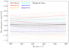 |
Fig. 9 Variation in the Hα absorption depth as a function of Kp. |
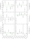 |
Fig. 10 Amplitude, centre, and FWHM values of the Gaussian fit performed on the Balmer Hα and Hβ lines for the average transmission spectrum obtained each night. No significant variations are present among the six transits, with the largest discrepancies in the absorption depth shown during night 2 (Hα, 1.8σ) and night 6 (Ηβ, 2.1σ). The full set of values is presented in Table A.1. |
χ2 and reduced χ2 ( ) values obtained from the comparison between the synthetic LTE and NLTE transmission spectra with the non-binned observations.
5.2 Ultraviolet to infrared transmission spectrum
To enable future comparisons with observations obtained in a broad range of wavelengths and by different facilities, we computed the synthetic NLTE and LTE transmission spectra ranging from the far-UV to the mid-infrared (i.e. from 912 Å to 2.85 μm). Figure 11 shows the LTE and NLTE synthetic transmission spectra across the whole considered wavelength range. Similar plots, but zooming into specific wavelength ranges for better visibility can be found in Appendix (Figs. A.10–A.15). For completeness and easier comparison with observations, we show in Fig. A.16 the transit depth difference between the theoretical LTE and NLTE transmission spectra.
Across the simulated wavelength range, the synthetic LTE transmission spectrum tends to underestimate the absorption, although there is a small sample of lines, mostly belonging to CaI and Fe-peak elements, where the LTE assumption overestimates the absorption. As for KELT-9b (Fossati et al. 2021), we find the strongest deviation from LTE in the UV band, with the deviation from LTE lying mostly between 5 and 15%, with a peak of about 17.5% for the Lyα line. on average, in the optical band the deviation from LTE is smaller and lies below 5%, but there are exceptions, such as the hydrogen Balmer lines where the deviation from LTE reaches between 10 and 15%. As in the case of KELT-9b (Fossati et al. 2021; Borsa et al. 2021b), the OI triplet at about 7780 Å shows a prominent deviation from LTE. However, in relation to the Hα line, the absorption depth of the oI triplet is smaller in this case compared to KELT-9b, which suggests that it might be harder to detect these lines in the atmosphere of KELT-20b/MASCARA-2b. The infrared band is dominated by the Paschen a line, for which we find a deviation from LTE of about 13%. The predicted absorption depth of this line is comparable to that of the Hγ and Hδ lines and might thus be detectable.
As described by Fossati et al. (2021), the strong difference between the theoretical LTE and NLTE transmission spectra, particularly in the UV wavelength range, is due to the difference in underlying TP profiles. Most of the spectral lines lying in the UV belong to ionised species, which are more abundant in the NLTE model as a consequence of the higher temperature of the NLTE TP profile compared to the LTE TP profile, particularly in the line forming region. Furthermore, the hotter temperature of the NLTE model leads to a higher pressure scale height compared to the LTE model, which also affects the absorption depth of the lines in the transmission spectrum.
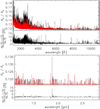 |
Fig. 11 Comparison between the theoretical LTE (red) and NLTE (black) transmission spectra. The top plot covers the UV and optical range, while the bottom plot covers the infrared band. The transmission spectra have been computed by applying a spectral resolution of 100 000. Within each plot, the bottom panel shows the deviation from LTE (in percent). |
5.3 Upper atmosphere
CLOUDY is a hydrostatic code and thus the fact that the composite theoretical TP profile produces a good fit to the observed hydrogen Balmer lines (see Fig. 8) implies that the atmosphere, at least in the line formation region and underneath it, is not in the hydrodynamic escape regime. In Fig. 12, we plot the theoretical sound speed (Cs) and the Jeans escape parameter as a function of pressure; the latter was calculated using Eq. (7) of Fossati et al. (2017, see also Volkov et al. 2011) for zero bulk flow velocity. This version of the Jeans escape parameter is based on the gravitational potential difference between a point in the atmosphere and the Roche lobe, which lies at about 9.5 RJ (i.e. about 5.2 Rp), and thus the Jeans escape parameter goes to zero at the Roche lobe. The Jeans escape parameter is well above 20 in the line formation region and thus any outflow in this region of the atmosphere is subsonic, explaining why the density profiles are close to hydrostatic (e.g. Koskinen et al. 2013). In agreement with Casasayas-Barris et al. (2019), we conclude that the Balmer lines do not directly constrain atmospheric escape and the planetary mass-loss rate.
5.4 Impact of planetary mass
The radial velocity measurements enabled one to set just an upper limit on the planetary mass. Therefore, we tested the impact of the choice of a planetary mass of 3.51 MJ (Borsa et al. 2022) on the main results. The top panel of Fig. 13 shows a comparison between the CLOUDY TP profiles computed considering a planetary mass equal to 2.5, 3.0, and 3.51 MJ. The three theoretical TP profiles are almost identical, which indicates that planetary mass has no impact on the obtained temperature structure. The profiles computed for 2.5 and 3.0 MJ do not extend in the upper atmosphere as much as that computed for 3.51 MJ, because of CLOUDY convergence problems at low pressures for the low-mass models.
We also computed HELIOS TP profiles assuming planetary masses of 2.5 and 3.0 MJ obtaining results essentially identical to those obtained for a planetary mass of 3.51 MJ. For each of the two additional values of the planetary mass, following the procedure described in Sect. 4.1 we combined the HELIOS and CLOUDY TP profiles to obtain the composite theoretical TP profile, and then we followed the procedure described in Sect. 5.1 to compute the synthetic transmission spectra. From the calibration of the transmission spectra to the observed planet-to-star radius ratio, we obtained a reference pressure value of 0.002 bar, which is the same as that we derived for a planetary mass of 3.51 MJ.
The middle panel of Fig. 13 shows the normalised Hα synthetic transmission spectra as a function of planetary mass, further comparing them to the observed profile. As expected, the line absorption depth increases with decreasing planetary mass and the higher considered mass of 3.51 MJ leads to a better fit to the data compared to what is obtained with lower masses. Under the assumption that the obtained theoretical TP profiles are representative of the planetary atmosphere, we conclude that the mass of KELT-20b/MASCARA-2b should lie between 3.0 and 3.51 MJ.
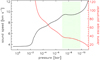 |
Fig. 12 Atmospheric sound speed (black; left y-axis) and Jeans escape parameter (red; right y-axis) profiles as a function of pressure computed on the basis of the composite TP profile. The hatched area indicates the Hα line formation region. |
6 Conclusions
We have presented the transmission spectrum of the UHJ KELT-20b/MASCARA-2b that covers the Hα, Ηβ, Ηγ, and Ηδ line profiles extracted from six transit observations obtained with the HARPS-N high-resolution spectrograph. The Hα, Hβ and Ηγ lines are definitely detected with absorption depths of 0.79±0.03% (1.25 Rp), 0.52±0.03% (1.17 Rp), and 0.39±0.06% (1.13 Rp), respectively, while the Ηδ line is detected at the ~4σ level with an absorption depth of 0.27±0.07% (1.09 Rp). Our observed Hα and Hβ line profiles are in agreement with those obtained by Casasayas-Barris et al. (2019) based on three transit observations. Ours is the first detection of the Ηγ and Ηδ lines in the atmosphere of KELT-20b/MASCARA-2b; the Ηδ line might be contaminated by a nearby FeI line.
We have also presented the results of forward modelling of the TP profile of the planetary atmosphere at the sub-stellar point, covering the 10 bar to 10−12 bar range. The results were computed by combining the HELIOS (LTE) and CLOUDY (NLTE) codes, thus accounting for NLTE effects in the middle and upper atmosphere. We find an isothermal temperature of ≈2200 K at pressures higher than ≈10−2 bar and of ≈7700 K at pressures lower than ≈10−8 bar; in between these pressure values, the temperature increases roughly linearly. From comparing the LTE and NLTE theoretical TP profiles, we find that accounting for NLTE effects leads to a temperature increase in the middle and upper atmosphere of up to about 3000 K. As was found for KELT-9b, the temperature inversion is caused by metal-line absorption of the stellar photons. Furthermore, the higher temperature of the NLTE TP profile, in comparison to the LTE one, is caused by the impact of NLTE effects on the level populations of Fe and Mg, which play a significant role in heating and cooling, respectively. This result supports the idea that accounting for Fe, Mg, and their level population is of critical importance for adequately modelling the atmospheric energy balance of UHJs. This agrees with the result of Nugroho et al. (2020) and Johnson et al. (2023), who looked for the signature of potential molecular species that might cause the temperature inversion, without finding it. Metals are the primary cause of the temperature inversion, and the impact of NLTE effects on those metals increases the magnitude of the temperature rise.
In the model of KELT-9b, the inclusion of NLTE effects leads to a temperature increase in the upper atmosphere of about 2000 K compared to the LTE profile (Fossati et al. 2021), while in the model of KELT-20b/MASCARA-2b, which is cooler and orbits a cooler host compared to KELT-9b, we find a temperature increase of about 3000 K. Comparisons of the departure coefficients computed for the two planets in the middle and upper atmosphere led us to conclude that this difference might be ascribed to a lack of cooling in the atmosphere of KELT-20b/MASCARA-2b, rather than to an increase in heating. Therefore, NLTE effects might also significantly impact the TP profile of planets cooler than UHJs. This calls for a dedicated parameter study to gain insight into the impact that the system parameters have on the deviation from LTE on the atmospheric TP profile.
We remark that the shape of the stellar spectral energy distribution is likely to play a fundamental role in the properties of the upper atmosphere of UHJs, and in particular on whether a planet hosts a hydrostatic or hydrodynamic atmosphere. Both KELT-9b and KELT-20b/MASCARA-2b host hydrostatic atmospheres, and the spectral lines lying in the optical range (including Hα) do not probe the exosphere and do not directly constrain mass loss. This is because both host stars are earlier than spectral type A3–A4 and thus do not have strong X-ray or EUV emission (Fossati et al. 2018). This prevents the atmospheric hydrogen, which is by far the most abundant element, from heating up significantly and thus prevents the upper atmosphere from reaching temperatures high enough to become hydrodynamic. Instead, for planets orbiting stars later than A3–A4, the X-ray and EUV irradiation is expected to be significant, which in turn leads to strong hydrogen heating and thus most likely to a hydrodynamic atmosphere. For this reason, the observations of planets orbiting stars earlier and later than A3–A4 should not be directly compared to infer general properties of planets orbiting early-type stars.
We employed the LTE and NLTE theoretical TP profiles to compute high-resolution synthetic transmission spectra, covering the UV to infrared wavelength range and thus including the hydrogen Balmer lines. We find that the NLTE synthetic transmission spectrum is a good fit to the observed Balmer lines, while, as a result of the cooler temperature structure, the LTE synthetic line profiles are systematically weaker than the observations. The synthetic NLTE profiles are slightly stronger and systematically broader than the observed ones, which is probably caused by the use of the sub-stellar TP profile as the underlying structure for computing transmission spectra that probe instead the terminator region. From comparing the theoretical LTE and NLTE transmission spectra over the entire considered wavelength range, we find the strongest deviation from LTE in the UV spectral band, while in the optical and infrared the hydrogen Balmer and Paschen lines present the strongest deviation from LTE.
Finally, we considered the NLTE atmospheric structure to compute the sound speed and the Jeans escape parameter across the planetary atmosphere. We find that the sound speed increases with decreasing pressure, up to a value of about 12 km s−1 at the top of our simulation domain. Instead, the Jeans escape parameter suggests that the planetary atmosphere remains hydrostatic within the entire simulated pressure range.
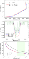 |
Fig. 13 Comparison between the CLOUDY TP profiles (top), normalised Hα transmission spectra (middle), and Jeans escape parameter (bottom) computed by setting the planetary mass equal to 3.51 MJ (black; Borsa et al. 2022), 2.5 MJ (red), and 3.0 MJ (blue). In the top panel, the TP profiles are rigidly shifted horizontally by the value indicated in the legend for visualisation purposes. In the middle panel, the green line shows the observed Hα transmission spectrum. |
Acknowledgements
This paper is based on observations collected with the 3.58 m Telescopio Nazionale Galileo (TNG), operated on the island of La Palma (Spain) by the Fundacion Galileo Galilei of the INAF (Istituto Nazionale di Astrofisica) at the Spanish observatorio del Roque de los Muchachos, in the frame of the programme Global Architecture of Planetary Systems (GAPS). This research used the facilities of the Italian Center for Astronomical Archive (IA2) operated by INAF at the Astronomical observatory of Trieste. We acknowledge support from PRIN INAF 2019. D.S. acknowledges funding from project PID2021-126365NB-C21(MCI/AEI/FEDER, UE) and financial support from the grant CEX2021-001131-S funded by MCIN/AEI/10.13039/501100011033. We thank the anonymous referee for the useful comments that led to improve the paper.
Appendix A Additional figures and table
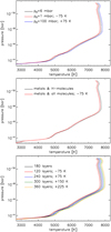 |
Fig. A.1 Comparison among TP profiles computed considering different assumptions for reference pressure, atmospheric composition, and number of layers. Top: Comparison between CLOUDY TP profiles obtained when fixing the planetary transit radius to the reference pressure (p0) values of 100 mbar (blue), 6 mbar (black), and 1 mbar (red). Middle: Comparison between CLOUDY TP profiles computed when accounting for metals plus only hydrogen molecules (black) and for metals plus all molecules present in the CLOUDY database (red). Bottom: Comparison between CLOUDY TP profiles obtained considering different numbers of layers, as indicated in the legend. For visualisation purposes, the TP profiles are rigidly shifted horizontally by the value indicated in the legend. |
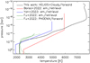 |
Fig. A.2 Comparison between our composite TP profile (black) with those published in the literature retrieved from secondary eclipse observations by Borsa et al. (2022, red), Yan et al. (2022, blue), and Fu et al. (2022, green). As a further comparison, the dashed green line shows the result of the forward model presented by Fu et al. (2022). We recall that the retrieved profiles are an average over the illuminated planet disk; the black line is computed for the sub-stellar point. |
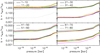 |
Fig. A.3 Departure coefficients as a function of pressure for the first 80 energy levels of FeI. The energy levels are numbered from 1 to 80, and are separated into groups of ten levels and two line styles (solid and dashed) for each panel. Within each group of ten energy levels, the order of the line colours corresponding to increasing energy is black, red, blue, dark green, magenta, yellow, brown, grey, bright green, and orange. The dotted line (at 1.0) indicating nNLTE = nLTE is for reference. |
Gaussian fit parameters for Hα and Hβ.
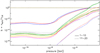 |
Fig. A.6 Same as Fig. A.3, but for MgII and up to the first 20 energy levels, which are those included in the 17.03 CLOUDY distribution. |
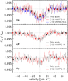 |
Fig. A.7 Comparison between our results obtained from combining six transits observed with HARPS-N (black) and that published by Casasayas-Barris et al. (2019) employing HARPS-N (three transits; red) and CARMENES (one transit; blue). The top, middle, and bottom panels show the comparison for the Hα, Hβ, and Ηγ lines, respectively. The central wavelengths of the Balmer lines (in vacuum) used to convert the wavelengths into velocities are 6564.60 Å for Hα, 4862.71 Å for Hβ, and 4341.69 Å for Ηγ. Lines correspond to the original data, while to guide the eye dots are the data binned to about 7.5 km s−1. The vertical and horizontal dotted lines respectively at zero and one are for reference. The HARPS-N transmission spectra of Casasayas-Barris et al. (2019) are about 20% noisier than those presented here. |
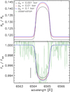 |
Fig. A.8 Comparison between CLOUDY synthetic transmission spectra of the Hα line before (top) and after (bottom) normalisation, computed considering different reference pressure levels at 0.001 bar (black), 0.01 bar (red), and 0.1 bar (blue). For reference, in the bottom panel the green line shows the observed Hα transmission spectrum, while the straight black line shows the average 1σ uncertainty obtained from the observations. Wavelengths are in vacuum. |
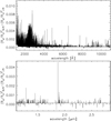 |
Fig. A.16 Transit depth difference between the NLTE and LTE transmission spectra shown in Fig. 11. The top plot covers the UV and optical range, while the bottom plot covers the infrared band. |
References
- Allart, R., Lovis, C., Pino, L., et al. 2017, A & A, 606, A144 [NASA ADS] [CrossRef] [EDP Sciences] [Google Scholar]
- Arcangeli, J., Désert, J.-M., Line, M. R., et al. 2018, ApJ, 855, L30 [Google Scholar]
- Bello-Arufe, A., Buchhave, L. A., Mendonça, J. M., et al. 2022, A & A, 662, A51 [NASA ADS] [CrossRef] [EDP Sciences] [Google Scholar]
- Borsa, F., & Zannoni, A. 2018, A & A, 617, A134 [NASA ADS] [CrossRef] [EDP Sciences] [Google Scholar]
- Borsa, F., Rainer, M., Bonomo, A. S., et al. 2019, A & A, 631, A34 [NASA ADS] [CrossRef] [EDP Sciences] [Google Scholar]
- Borsa, F., Allart, R., Casasayas-Barris, N., et al. 2021a, A & A, 645, A24 [NASA ADS] [CrossRef] [EDP Sciences] [Google Scholar]
- Borsa, F., Fossati, L., Koskinen, T., Young, M. E., & Shulyak, D. 2021b, Nat. Astron., 6, 226 [Google Scholar]
- Borsa, F., Giacobbe, P., Bonomo, A. S., et al. 2022, A & A, 663, A141 [NASA ADS] [CrossRef] [EDP Sciences] [Google Scholar]
- Casasayas-Barris, N., Pallé, E., Yan, F., et al. 2018, A & A, 616, A151 [CrossRef] [EDP Sciences] [Google Scholar]
- Casasayas-Barris, N., Pallé, E., Yan, F., et al. 2019, A & A, 628, A9 [NASA ADS] [CrossRef] [EDP Sciences] [Google Scholar]
- Casasayas-Barris, N., Pallé, E., Yan, F., et al. 2020, A & A, 635, A206 [NASA ADS] [CrossRef] [EDP Sciences] [Google Scholar]
- Cont, D., Yan, F., Reiners, A., et al. 2022, A & A, 657, A2 [Google Scholar]
- Cosentino, R., Lovis, C., Pepe, F., et al. 2012, SPIE Conf. Ser., 8446, 84461V [Google Scholar]
- Del Pozzo, W., & Veitch, J. 2022, CPNest: Parallel nested sampling, Astrophysics Source Code Library, [record ascl:2205.021] [Google Scholar]
- Ehrenreich, D., Lovis, C., Allart, R., et al. 2020, Nature, 580, 597 [Google Scholar]
- Ferland, G. J., Korista, K. T., Verner, D. A., et al. 1998, PASP, 110, 761 [Google Scholar]
- Ferland, G. J., Porter, R. L., van Hoof, P. A. M., et al. 2013, Rev. Mexicana Astron. Astrofis., 49, 137 [Google Scholar]
- Ferland, G. J., Chatzikos, M., Guzmán, F., et al. 2017, Rev. Mexicana Astron. Astrofis., 53, 385 [Google Scholar]
- Fossati, L., Erkaev, N. V., Lammer, H., et al. 2017, A & A, 598, A90 [NASA ADS] [CrossRef] [EDP Sciences] [Google Scholar]
- Fossati, L., Koskinen, T., Lothringer, J. D., et al. 2018, ApJ, 868, L30 [CrossRef] [Google Scholar]
- Fossati, L., Shulyak, D., Sreejith, A. G., et al. 2020, A & A, 643, A131 [NASA ADS] [CrossRef] [EDP Sciences] [Google Scholar]
- Fossati, L., Young, M. E., Shulyak, D., et al. 2021, A & A, 653, A52 [NASA ADS] [CrossRef] [EDP Sciences] [Google Scholar]
- Fu, G., Sing, D. K., Lothringer, J. D., et al. 2022, ApJ, 925, L3 [NASA ADS] [CrossRef] [Google Scholar]
- García Muñoz, A., & Schneider, P. C. 2019, ApJ, 884, L43 [Google Scholar]
- Gaudi, B. S., Stassun, K. G., Collins, K. A., et al. 2017, Nature, 546, 514 [NASA ADS] [Google Scholar]
- Giacobbe, P., Brogi, M., Gandhi, S., et al. 2021, Nature, 592, 205 [NASA ADS] [CrossRef] [Google Scholar]
- Guilluy, G., Giacobbe, P., Carleo, I., et al. 2022, A & A, 665, A104 [NASA ADS] [CrossRef] [EDP Sciences] [Google Scholar]
- Hoeijmakers, H. J., Ehrenreich, D., Heng, K., et al. 2018, Nature, 560, 453 [CrossRef] [Google Scholar]
- Hoeijmakers, H. J., Ehrenreich, D., Kitzmann, D., et al. 2019, A & A, 627, A165 [NASA ADS] [CrossRef] [EDP Sciences] [Google Scholar]
- Hoeijmakers, H. J., Cabot, S. H. C., Zhao, L., et al. 2020, A & A, 641, A120 [NASA ADS] [CrossRef] [EDP Sciences] [Google Scholar]
- Husser, T. O., Wende-von Berg, S., Dreizler, S., et al. 2013, A & A, 553, A6 [NASA ADS] [CrossRef] [EDP Sciences] [Google Scholar]
- Johnson, M. C., Wang, J., Pai Asnodkar, A., et al. 2023, AJ, 165, 157 [NASA ADS] [CrossRef] [Google Scholar]
- Kasper, D., Bean, J. L., Line, M. R., et al. 2023, AJ, 165, 7 [NASA ADS] [CrossRef] [Google Scholar]
- Kausch, W., Noll, S., Smette, A., et al. 2015, A & A, 576, A78 [NASA ADS] [CrossRef] [EDP Sciences] [Google Scholar]
- Kesseli, A. Y., & Snellen, I. A. G. 2021, ApJ, 908, L17 [Google Scholar]
- Kesseli, A. Y., Snellen, I. A. G., Alonso-Floriano, F. J., Mollière, P., & Serindag, D. B. 2020, AJ, 160, 228 [NASA ADS] [CrossRef] [Google Scholar]
- Koskinen, T. T., Yelle, R. V., Harris, M. J., & Lavvas, P. 2013, Icarus, 226, 1695 [NASA ADS] [CrossRef] [Google Scholar]
- Lodders, K. 2003, ApJ, 591, 1220 [Google Scholar]
- Lothringer, J. D., & Barman, T. 2019, ApJ, 876, 69 [Google Scholar]
- Lothringer, J. D., Barman, T., & Koskinen, T. 2018, ApJ, 866, 27 [NASA ADS] [CrossRef] [Google Scholar]
- Lund, M. B., Rodriguez, J. E., Zhou, G., et al. 2017, AJ, 154, 194 [Google Scholar]
- Malik, M., Grosheintz, L., Mendonça, J. M., et al. 2017, AJ, 153, 56 [Google Scholar]
- Malik, M., Kitzmann, D., Mendonça, J. M., et al. 2019, AJ, 157, 170 [Google Scholar]
- Nugroho, S. K., Gibson, N. P., de Mooij, E. J. W., et al. 2020, MNRAS, 496, 504 [Google Scholar]
- Pino, L., Désert, J.-M., Brogi, M., et al. 2020, ApJ, 894, L27 [Google Scholar]
- Piskunov, N., & Valenti, J. A. 2017, A & A, 597, A16 [NASA ADS] [CrossRef] [EDP Sciences] [Google Scholar]
- Rainer, M., Borsa, F., Pino, L., et al. 2021, A & A, 649, A29 [NASA ADS] [CrossRef] [EDP Sciences] [Google Scholar]
- Ryabchikova, T., Piskunov, N., Kurucz, R. L., et al. 2015, Physica Scripta, 90, 054005 [NASA ADS] [CrossRef] [Google Scholar]
- Sicilia, D., Malavolta, L., Pino, L., et al. 2022, A & A, 667, A19 [NASA ADS] [CrossRef] [EDP Sciences] [Google Scholar]
- Skilling, J. 2006, Bayesian Anal., 1, 833 [Google Scholar]
- Smette, A., Sana, H., Noll, S., et al. 2015, A & A, 576, A77 [NASA ADS] [CrossRef] [EDP Sciences] [Google Scholar]
- Stangret, M., Casasayas-Barris, N., Pallé, E., et al. 2020, A & A, 638, A26 [NASA ADS] [CrossRef] [EDP Sciences] [Google Scholar]
- Stock, J. W., Kitzmann, D., Patzer, A. B. C., & Sedlmayr, E. 2018, MNRAS, 479, 865 [NASA ADS] [Google Scholar]
- Talens, G. J. J., Spronck, J. F. P., Lesage, A. L., et al. 2017, A & A, 601, A11 [NASA ADS] [CrossRef] [EDP Sciences] [Google Scholar]
- Talens, G. J. J., Justesen, A. B., Albrecht, S., et al. 2018, A & A, 612, A57 [NASA ADS] [CrossRef] [EDP Sciences] [Google Scholar]
- Turner, O. D., Anderson, D. R., Barkaoui, K., et al. 2019, MNRAS, 485, 5790 [NASA ADS] [CrossRef] [Google Scholar]
- Turner, J. D., de Mooij, E. J. W., Jayawardhana, R., et al. 2020, ApJ, 888, L13 [Google Scholar]
- Volkov, A. N., Johnson, R. E., Tucker, O. J., & Erwin, J. T. 2011, ApJ, 729, L24 [Google Scholar]
- Wyttenbach, A., Ehrenreich, D., Lovis, C., Udry, S., & Pepe, F. 2015, A & A, 577, A62 [NASA ADS] [CrossRef] [EDP Sciences] [Google Scholar]
- Wyttenbach, A., Mollière, P., Ehrenreich, D., et al. 2020, A & A, 638, A87 [NASA ADS] [CrossRef] [EDP Sciences] [Google Scholar]
- Yan, F., Pallé, E., Fosbury, R. A. E., Petr-Gotzens, M. G., & Henning, T. 2017, A & A, 603, A73 [NASA ADS] [CrossRef] [EDP Sciences] [Google Scholar]
- Yan, F., Casasayas-Barris, N., Molaverdikhani, K., et al. 2019, A & A, 632, A69 [CrossRef] [EDP Sciences] [Google Scholar]
- Yan, F., Reiners, A., Pallé, E., et al. 2022, A & A, 659, A7 [NASA ADS] [CrossRef] [EDP Sciences] [Google Scholar]
- Young, M. E., Fossati, L., Koskinen, T. T., et al. 2020, A & A, 641, A47 [NASA ADS] [CrossRef] [EDP Sciences] [Google Scholar]
We specified the use of an intrinsic scatter in the fit model to take into account the noise present in the data.
All Tables
χ2 and reduced χ2 () values obtained from the comparison between the synthetic LTE and NLTE transmission spectra with the non-binned observations.
All Figures
|
Fig. 1 Example of MOLECFIT tellurics correction in the proximity of the Hα line. |
| In the text | |
|
Fig. 2 Theoretical atmospheric structure obtained for KELT-20b/MASCARA-2b. Top: HELIOS (dashed orange line) and CLOUDY (in NLTE; dashed cyan line) TP profiles. The solid black line shows the composite TP profile. The horizontal dotted black line indicates the location of the continuum according to the HELIOS model. The horizontal dash-dotted red line gives the location of the CLOUDY’s upper-density limit of 1015 cm−3. The dashed dark green line shows the CLOUDY TP profile computed assuming LTE. The hatched area indicates the Hα line formation region. Bottom: pressure (black; left y-axis) and temperature (red; right y-axis) composite theoretical profiles as a function of the planetary polar radius. |
| In the text | |
|
Fig. 3 Density relative to the total density of hydrogen for neutral hydrogen (HI; solid black line), protons (HII~; red), molecular hydrogen (H2; dark green), |
| In the text | |
|
Fig. 4 Atmospheric mixing ratios obtained for metals. Top: mixing ratios for hydrogen (solid black line), H2 (dotted black), He (red), C (blue), O (dark green), Na (violet), K (orange), and electrons (bright green) as a function of atmospheric pressure. Neutral (XI), singly ionised (XII), and doubly ionised (XIII) species are shown as solid, dashed, and dash-dotted lines, respectively. Bottom: same as the top panel, but for Mg (red), Si (blue), Ca (dark green), and Fe (violet). The hydrogen, H2, and e− mixing ratios are shown in both panels for reference. |
| In the text | |
|
Fig. 5 Comparison between the NLTE CLOUDY TP profiles obtained considering all elements up to Zn (solid black line) and excluding Fe (solid red line) or Mg (solid blue line). The dashed orange line shows the HELIOS (i.e. LTE) TP profile for reference. |
| In the text | |
|
Fig. 6 Heating and cooling contributions in the atmosphere of KELT-20b/MASCARA-2b. Top: contribution to the total heating as a function of pressure. At each pressure bin, the plot shows the three most important heating processes. The main heating processes occurring in the middle and upper atmosphere are hydrogen photoionisation (red; photoionisation of HI lying in the ground state), metal line absorption (blue), H− absorption (green), photoionisation of hydrogenic species (photoionisation of excited HI; magenta), and collisions with H2 (brown). Bottom: contribution to the total cooling as a function of pressure. At each pressure bin, the plot shows the three most important cooling agents. |
| In the text | |
|
Fig. 7 Atmospheric structure and heating rate obtained from isolating the impacts of Fe and Mg ions. Top: temperature (left) and total heating rate (right) as a function of pressure obtained accounting for all elements (black; same as in Figs. 2 and 5), considering that in the planetary atmosphere Fe exists only in the form of FeI (blue), only in the form of FeII (green), or is absent (i.e. no Fe; same as Fig. 5; red). Bottom: same as the top, but for Mg. |
| In the text | |
|
Fig. 8 Comparison between observed and synthetic Hα (top left), Bβ (top right), Ηγ (bottom left), and Hδ (bottom right) line profiles. The solid black line shows the observations, while to guide the eye the black dots show the observed profiles re-binned to about 4.5 km s−1. The dashed red line indicates the Gaussian fit to the observations. The solid blue and dash-dotted green lines show the CLOUDY synthetic line profiles computed in NLTE and LTE, respectively. The central wavelengths of the Balmer lines (in vacuum) used to convert the wavelengths into velocities are 6564.60 Å for Hα, 4862.71 Å for Hβ, 4341.69 Å for Ηγ, and 4102.892 Å for Hδ. |
| In the text | |
|
Fig. 9 Variation in the Hα absorption depth as a function of Kp. |
| In the text | |
|
Fig. 10 Amplitude, centre, and FWHM values of the Gaussian fit performed on the Balmer Hα and Hβ lines for the average transmission spectrum obtained each night. No significant variations are present among the six transits, with the largest discrepancies in the absorption depth shown during night 2 (Hα, 1.8σ) and night 6 (Ηβ, 2.1σ). The full set of values is presented in Table A.1. |
| In the text | |
|
Fig. 11 Comparison between the theoretical LTE (red) and NLTE (black) transmission spectra. The top plot covers the UV and optical range, while the bottom plot covers the infrared band. The transmission spectra have been computed by applying a spectral resolution of 100 000. Within each plot, the bottom panel shows the deviation from LTE (in percent). |
| In the text | |
|
Fig. 12 Atmospheric sound speed (black; left y-axis) and Jeans escape parameter (red; right y-axis) profiles as a function of pressure computed on the basis of the composite TP profile. The hatched area indicates the Hα line formation region. |
| In the text | |
|
Fig. 13 Comparison between the CLOUDY TP profiles (top), normalised Hα transmission spectra (middle), and Jeans escape parameter (bottom) computed by setting the planetary mass equal to 3.51 MJ (black; Borsa et al. 2022), 2.5 MJ (red), and 3.0 MJ (blue). In the top panel, the TP profiles are rigidly shifted horizontally by the value indicated in the legend for visualisation purposes. In the middle panel, the green line shows the observed Hα transmission spectrum. |
| In the text | |
|
Fig. A.1 Comparison among TP profiles computed considering different assumptions for reference pressure, atmospheric composition, and number of layers. Top: Comparison between CLOUDY TP profiles obtained when fixing the planetary transit radius to the reference pressure (p0) values of 100 mbar (blue), 6 mbar (black), and 1 mbar (red). Middle: Comparison between CLOUDY TP profiles computed when accounting for metals plus only hydrogen molecules (black) and for metals plus all molecules present in the CLOUDY database (red). Bottom: Comparison between CLOUDY TP profiles obtained considering different numbers of layers, as indicated in the legend. For visualisation purposes, the TP profiles are rigidly shifted horizontally by the value indicated in the legend. |
| In the text | |
|
Fig. A.2 Comparison between our composite TP profile (black) with those published in the literature retrieved from secondary eclipse observations by Borsa et al. (2022, red), Yan et al. (2022, blue), and Fu et al. (2022, green). As a further comparison, the dashed green line shows the result of the forward model presented by Fu et al. (2022). We recall that the retrieved profiles are an average over the illuminated planet disk; the black line is computed for the sub-stellar point. |
| In the text | |
|
Fig. A.3 Departure coefficients as a function of pressure for the first 80 energy levels of FeI. The energy levels are numbered from 1 to 80, and are separated into groups of ten levels and two line styles (solid and dashed) for each panel. Within each group of ten energy levels, the order of the line colours corresponding to increasing energy is black, red, blue, dark green, magenta, yellow, brown, grey, bright green, and orange. The dotted line (at 1.0) indicating nNLTE = nLTE is for reference. |
| In the text | |
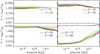 |
Fig. A.4 Same as Fig. A.3, but for FeII. |
| In the text | |
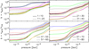 |
Fig. A.5 Same as Fig. A.3, but for MgI. |
| In the text | |
|
Fig. A.6 Same as Fig. A.3, but for MgII and up to the first 20 energy levels, which are those included in the 17.03 CLOUDY distribution. |
| In the text | |
|
Fig. A.7 Comparison between our results obtained from combining six transits observed with HARPS-N (black) and that published by Casasayas-Barris et al. (2019) employing HARPS-N (three transits; red) and CARMENES (one transit; blue). The top, middle, and bottom panels show the comparison for the Hα, Hβ, and Ηγ lines, respectively. The central wavelengths of the Balmer lines (in vacuum) used to convert the wavelengths into velocities are 6564.60 Å for Hα, 4862.71 Å for Hβ, and 4341.69 Å for Ηγ. Lines correspond to the original data, while to guide the eye dots are the data binned to about 7.5 km s−1. The vertical and horizontal dotted lines respectively at zero and one are for reference. The HARPS-N transmission spectra of Casasayas-Barris et al. (2019) are about 20% noisier than those presented here. |
| In the text | |
|
Fig. A.8 Comparison between CLOUDY synthetic transmission spectra of the Hα line before (top) and after (bottom) normalisation, computed considering different reference pressure levels at 0.001 bar (black), 0.01 bar (red), and 0.1 bar (blue). For reference, in the bottom panel the green line shows the observed Hα transmission spectrum, while the straight black line shows the average 1σ uncertainty obtained from the observations. Wavelengths are in vacuum. |
| In the text | |
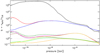 |
Fig. A.9 Same as Fig. A.3, but for the first ten energy levels of HI. |
| In the text | |
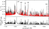 |
Fig. A.10 Same as Fig. 11, but for the 1100–1550Å band. |
| In the text | |
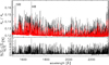 |
Fig. A.11 Same as Fig. 11, but for the 1500–2350Å band. |
| In the text | |
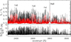 |
Fig. A.12 Same as Fig. 11, but for the 2300–3050Å band. |
| In the text | |
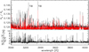 |
Fig. A.13 Same as Fig. 11, but for the 3000–4050Å band. |
| In the text | |
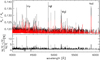 |
Fig. A.14 Same as Fig. 11, but for the 4000–6100Å band. |
| In the text | |
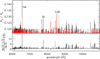 |
Fig. A.15 Same as Fig. 11, but for the 6000–11000Å band. |
| In the text | |
|
Fig. A.16 Transit depth difference between the NLTE and LTE transmission spectra shown in Fig. 11. The top plot covers the UV and optical range, while the bottom plot covers the infrared band. |
| In the text | |
Current usage metrics show cumulative count of Article Views (full-text article views including HTML views, PDF and ePub downloads, according to the available data) and Abstracts Views on Vision4Press platform.
Data correspond to usage on the plateform after 2015. The current usage metrics is available 48-96 hours after online publication and is updated daily on week days.
Initial download of the metrics may take a while.