| Issue |
A&A
Volume 692, December 2024
|
|
|---|---|---|
| Article Number | A79 | |
| Number of page(s) | 22 | |
| Section | Extragalactic astronomy | |
| DOI | https://doi.org/10.1051/0004-6361/202451207 | |
| Published online | 03 December 2024 | |
TODDLERS: A new UV-millimeter emission library for star-forming regions
II. Star-formation rate indicators using Auriga zoom simulations
1
Sterrenkundig Observatorium, Universiteit Gent, Krijgslaan 281-S9, B-9000 Gent, Belgium
2
The University of Texas at Dallas, 800 W Campbell Rd, Richardson, TX 75080, USA
3
Faculté des sciences et de génie, Université Laval, Pavillon Alexandre-Vachon, Québec G1V 0A6, Canada
4
Université Côte d’Azur, Observatoire de la Côte d’Azur, CNRS, Laboratoire Lagrange, F-06000 Nice, France
⋆ Corresponding author; This email address is being protected from spambots. You need JavaScript enabled to view it.
Received:
21
June
2024
Accepted:
21
October
2024
Abstract
Context. The current generation galaxy formation simulations often approximate star formation, making it necessary to use models of star-forming regions to produce observables from such simulations. In the first paper of this series, we introduced TODDLERS, a physically motivated, time-resolved model for UV–millimeter (mm) emission from star-forming regions, implemented within the radiative transfer code SKIRT. In this work, we use the SKIRT-TODDLERS pipeline to produce synthetic observations.
Aims. We aim to demonstrate the potential of TODDLERS model through observables and quantities pertaining to star-formation. An additional goal is to compare the results obtained using TODDLERS with the existing star-forming regions model in SKIRT.
Methods. We calculated broadband and line emission maps for the 30 Milky Way-like galaxies of the Auriga zoom simulation suite at a redshift of zero. Analyzing far-ultraviolet (FUV) and infrared (IR) broadband data, we calculated kiloparsec (kpc)-resolved IR correction factors, kIR, which allowed us to quantify the ratio of FUV luminosity absorbed by dust to reprocessed IR luminosity. Furthermore, we used the IR maps to calculate the kpc-scale mid-infrared (MIR) colors (8 μm/24 μm) and far-infrared (FIR) colors (70 μm/500 μm) of the Auriga galaxies. We used Hα and Hβ line maps to study the Balmer decrement and dust correction. We verified the fidelity of our model’s FIR fine structure lines as star formation rate (SFR) indicators.
Results. The integrated UV-mm spectral energy distributions (SEDs) exhibit higher FUV and near-ultraviolet (NUV) attenuation and lower 24 μm emission compared to the existing star-forming regions model in SKIRT, alleviating tensions with observations reported in earlier studies. The light-weighted mean kIR increases with aperture and inclination, while its correlation with kpc-resolved specific star-formation rate (sSFR) is weaker than literature values from resolved SED fitting, potentially due to inaccuracies in local energy balance representation. The kpc-scale MIR-FIR colors show an excellent agreement with local observational data, with anti-correlation degree varying by galaxy morphology. We find that the Balmer decrement effectively corrects for dust, with the attenuation law varying with dust amount. The Hα emission attenuation levels in our models are comparable to those observed in the high-density regions of state-of-the-art radiation hydrodynamical simulations. The FIR fine-structure line emission-based luminosity-SFR relations are consistent with global observational relations, with the [C II] line displaying the best agreement.
Key words: radiative transfer / methods: numerical / dust / extinction / HII regions / ISM: lines and bands / galaxies: ISM
© The Authors 2024
 Open Access article, published by EDP Sciences, under the terms of the Creative Commons Attribution License (https://creativecommons.org/licenses/by/4.0), which permits unrestricted use, distribution, and reproduction in any medium, provided the original work is properly cited.
This article is published in open access under the Subscribe to Open model. This email address is being protected from spambots. You need JavaScript enabled to view it. to support open access publication.
1. Introduction
Star formation is a fundamental phenomenon in astrophysics, crucial for shaping the evolution of galaxies (Kennicutt 1998). This process transforms dust and gas within molecular clouds into stars, injecting chemical elements and energy into the interstellar medium (ISM; McKee & Ostriker 2007; Krumholz 2014; Chevance et al. 2020). Young, massive stars at star-forming sites play a crucial role in shaping a galaxy’s spectral energy distribution (SED), producing some of the most prominent observational signatures across wavelengths (Churchwell et al. 2006, 2007; Hanaoka et al. 2019; Tacchella et al. 2023). Emission from recent star formation dominates the UV output of galaxies (Salim et al. 2007; Gil de Paz et al. 2007; Hao et al. 2011; Robotham & Driver 2011), while reprocessed emission by dust creates prominent infrared (IR) features (Calzetti et al. 2000; Rieke et al. 2009; Kennicutt & Evans 2012). Furthermore, massive stars emit radiation that ionizes the surrounding gas, leading to the production of recombination emission lines such as Hα and Hβ (Leitherer et al. 1999; Osterbrock & Ferland 2006). These lines (in)directly trace the ionizing radiation output of young, massive stars. The energetic free electrons produced through ionization heat the gas, and the subsequent cooling through metal emission also leaves important observational signatures (Rubin 1985; Ferland et al. 1998). These emission features serve as crucial tools for uncovering the physical conditions and chemical makeup of the ISM, providing valuable insights into galaxy formation and evolution (Kewley & Dopita 2002; Kewley et al. 2019; Nakajima & Maiolino 2022; Crain & van de Voort 2023).
On the theoretical front, hydrodynamical numerical simulations have become indispensable in the study of galaxy formation and evolution (Somerville & Davé 2015; Vogelsberger et al. 2020a). The scale of the model significantly influences its focus and complexity, necessitating the use of sub-grid models to approximate unresolved phenomena such as star formation, stellar feedback, and the interaction of energy and matter on scales smaller than can be directly simulated. Currently, some state-of-the-art isolated galaxy simulations are able to achieve a parsec-scale (pc-scale) resolution, allowing them to resolve cold molecular gas in regions where stars are born. Notable works in this direction include Smith et al. (2018), Marinacci et al. (2019), Kannan et al. (2020), Feldmann et al. (2023), Katz et al. (2022), Richings et al. (2022), Steinwandel et al. (2024), and Deng et al. (2024). Although the detailed processes of star formation are realized through sub-grid models, these high-resolution simulations represent the most realistic current models of the influence of stellar feedback on the surrounding gas in galaxy simulations. On the other hand, simulations that encompass a larger number of galaxies enable the study of galaxy formation and evolution in a cosmological context. These efforts generally come in two guises. Some directly simulate a large co-moving volume, such as Illustris (Vogelsberger et al. 2014), EAGLE (Crain et al. 2017), Simba (Davé et al. 2019), IllustrisTNG (Pillepich et al. 2019), and NewHorizon (Dubois et al. 2021). Others zoom in on interesting regions or halos with specific characteristics, using a higher number of resolution elements, such as NIHAO (Wang et al. 2015a), Auriga (Grand et al. 2017), ARTEMIS (Font et al. 2020), THE THREE HUNDRED project (Cui et al. 2022), and HELLO project (Waterval et al. 2024). In both cases, due to limitations in the physical modeling, resolution constraints, or the high computational cost from very small time steps in dense gas regions, approximate treatments of the ISM are necessary. These approximations often result in an ISM that is highly unresolved and overly smooth. Common techniques include implementing an effective equation of state and/or artificial temperature as well as pressure floors to prevent unresolved numerical fragmentation and maintain computational stability (Springel & Hernquist 2003; Schaye et al. 2015; Inoue & Yoshida 2019). While these approaches enable the simulation of larger volumes or higher resolution in specific regions, they significantly impact the modeled ISM structure, limiting the ability to resolve its cold, dense phases. Furthermore, the use of such methods fundamentally changes the behavior of mechanical, chemical, radiative, and thermodynamical feedback processes. As a result, simulated galaxies frequently display smoother structures on scales of several hundred parsecs and tend to be thicker and kinematically hotter than observed (Marinacci et al. 2019; Benítez-Llambay et al. 2018). Thus, these simulations are unable to capture detailed small-scale information about star-forming environments, including the intricate physical conditions such as gas density, temperature, and chemical composition. These gas conditions are critical for determining the emission from star-forming regions as they influence the ionization states and excitation mechanisms (Osterbrock & Ferland 2006; Draine 2011; Ryden & Pogge 2021).
While efforts to simulate the multi-phase ISM continue for the next generation of cosmological simulations (see, e.g., Ploeckinger & Schaye 2020; Chaikin et al. 2023), the production of synthetic observations using current-generation large-volume simulations requires sub-grid models to incorporate small-scale gas emission, such as those from star-forming regions. This helps ensure a proper accounting of the complex interplay of physical processes at smaller scales. Such an approach bridges the gap between large-scale cosmological simulations and the small-scale information required for predicting emissions from star-forming regions. Several examples in the literature use this method to predict individual line luminosities (Olsen et al. 2017; Pellegrini et al. 2020; Olsen et al. 2021; Hirschmann et al. 2023; Garg et al. 2022). However, there is a dearth of models that predict both continuum and line-emission from UV to millimeter wavelengths as this requires combining multiple specialty radiative transfer techniques. Our work is dedicated to such multi-wavelength modeling in the context of high-resolution hydrodynamical simulations. By adopting this approach, we aim to enhance the predictive power of current-generation simulations, striving for greater realism while maintaining similar computational efforts.
In Kapoor et al. (2023, hereafter Paper I), we introduced a physically motivated, time-resolved representation of UV to millimeter (UV–mm) emission from star-forming regions, including both emission lines and continua. The model was constructed using a 1D evolution model for a spherical, homogeneous gas cloud exposed to stellar feedback, coupled with the photoionization code Cloudy. The inclusion of the TODDLERS library in SKIRT, a state-of-the-art three-dimensional (3D) multi-physics Monte Carlo radiative transfer code, facilitates forward modeling of cosmological hydrodynamical simulations. This integration provides meaningful insights from the complex observations made by integral field unit (IFU) instruments. This is particularly relevant and timely given the increasing number of advanced IFU instruments such as Multi Unit Spectroscopic Explorer (MUSE; Bacon et al. 2010) on the Very Large Telescope (VLT), Atacama Large Millimeter/submillimeter Array (ALMA; Wootten & Thompson 2009), James Webb Space Telescope (JWST; Gardner et al. 2006), and Spectromètre ImageuràTransformée de Fourier pour l’Etude en Long et en Large de raies d’Emission (SITELLE; Drissen et al. 2019) on the Canada-France-Hawaii Telescope (CFHT) are actively gathering data, allowing for spectrally and spatially resolved observations, enabling comprehensive mapping of galaxy properties. While Paper I laid the foundations of this investigation by detailing the methodology, key diagnostics, and comparisons with state-of-the-art models (such as the one presented in Groves et al. 2008, referred to as HiiM3 for the version available in SKIRT), this work focuses on applying the TODDLERS library to generate synthetic observables using the Auriga suite of simulations (Grand et al. 2017). Through an exploration of broadband images, optical, and FIR spectra, we aim to demonstrate the capabilities and potential of the TODDLERS model and provide a detailed comparison of the synthetic data with observations to validate our approach.
In Sect. 2, we provide background information on the Auriga simulations, the DustPedia project, the SKIRT radiative transfer code, and the TODDLERS model, which comprise the tools and datasets used in our study. In Sect. 3, we describe the process of exporting Auriga snapshots to SKIRT for performing the RT simulations and the calibration of the free parameters for accurate physical modeling. Section 4 describes the data products generated in this work. In Sect. 5, we compare the Auriga SEDs obtained using TODDLERS in the post-processing pipeline with those obtained using HiiM3. We also analyze the broadband images generated in this work, focusing on hybrid UV-IR star-formation rate (SFR) indicators and mid-infrared-far-infrared (MIR-FIR) colors to evaluate their utility and correspondence to observed galaxy properties. In Sect. 6, we discuss and present the analysis of the Balmer and FIR fine-structure line emission of Auriga galaxies using TODDLERS. Finally, in Sect. 7, we summarize our findings, present our conclusions, and suggest directions for future research and applications.
2. Background
2.1. Auriga simulations
Auriga (Grand et al. 2017, 2024) is a set of 30 zoom simulations aimed at the modeling of Milky Way-type galaxies in a full cosmological context, carried out using the moving-mesh magnetohydrodynamics (MHD) code AREPO (Springel 2010). These simulations follow a Λ cold dark matter cosmology consistent with the Planck Collaboration Int. XVI (2014) data release. The host dark matter halos of the zoomed galaxy simulations were drawn from a dark-matter-only simulation of a comoving side length of 100 cMpc, with selection criteria on the mass and the isolation of the host halos. The virial mass ranges between 1 and 2 times 1012 M⊙, consistent with recent determinations of the Milky Way mass (see Wang et al. 2015b, and references therein).
The Auriga physics model uses primordial and metal-line cooling with self-shielding corrections. A spatially uniform UV background field (Faucher-Giguère et al. 2009) is employed. The ISM is modeled with a two-phase equation of state from Springel & Hernquist (2003). Star formation proceeds stochastically in gas with densities higher than a threshold density (nthr = 0.13 cm−3). The star formation probability in the candidate gas cells scales exponentially with time, with a characteristic time scale of tSF = 2.2 Gyr. The single stellar population (SSP) of each star particle is represented by the Chabrier (2003) initial mass function (IMF). Mass and metal returns from Type Ia supernovae (SNIa), asymptotic giant branch (AGB), and Type II supernovae (SNII) stars are calculated at each time step and are distributed among nearby gas cells with a top-hat kernel. The number of SNII events equals the number of stars in an SSP that lie in the mass range 8−100 M⊙. The model includes gas accretion by black holes, with active galactic nucleus (AGN) feedback in radio and quasar modes, both of which are always active and are thermal in nature. Magnetic fields are treated with ideal MHD following Pakmor & Springel (2013).
2.2. DustPedia project
The DustPedia galaxy sample (Davies et al. 2017) contains 875 nearby galaxies with matched aperture photometry in more than 40 bands from UV to millimeter wavelengths (Clark et al. 2018). The DustPedia galaxy sample covers a broad dynamic range of various physical properties, including stellar mass, SFR, and morphological stage, making it representative for galaxies in the local Universe. The observed and inferred physical properties of the DustPedia galaxies have studied in detail using various techniques (e.g., Casasola et al. 2017, 2020, 2022; Bianchi et al. 2018; De Vis et al. 2019; Nersesian et al. 2019, 2020). The sample is therefore ideal for a comparison between observed and simulated galaxies at z ∼ 0, as has been used in this way by various authors (Trčka et al. 2020; Kapoor et al. 2021; Camps et al. 2022). Here we follow the same approach as in Kapoor et al. (2021, hereafter referred to as K21), using the DustPedia data set to calibrate the RT post-processing recipe for the simulated Auriga galaxies (as described in Sect. 3.6).
2.3. SKIRT radiative transfer code
The 3D Monte Carlo radiative transfer code SKIRT (Baes et al. 2011; Camps & Baes 2015, 2020) is capable of importing the output from various kinds of hydrodynamical simulations. It contains a hybrid parallelization strategy (Verstocken et al. 2017), a library of flexible input models (Baes & Camps 2015), and a suite of advanced spatial grids for discretizing the medium (Camps et al. 2013; Saftly et al. 2014; Lauwers et al. 2024). It simulates the absorption, scattering, and thermal emission by dust grains, including stochastic heating (Camps et al. 2015) and support for kinematics (Camps & Baes 2020; Barrientos Acevedo et al. 2023) and polarisation (Peest et al. 2017; Vandenbroucke et al. 2021). Apart from dust radiative transfer, the code is designed to perform Lyman-α radiative transfer (Camps et al. 2021), X-ray radiative transfer (Vander Meulen et al. 2023), 21 centimeter (cm) hydrogen radiative transfer (Gebek et al. 2023), and non-local thermodynamic equilibrium (non-LTE) line radiative transfer (Matsumoto et al. 2023) without any constraints on geometrical complexity.
The code has been extensively used to generate line-emission maps, synthetic UV to submm broadband images, spectral energy distributions, and polarisation maps for idealized galaxies (Gadotti et al. 2010; Peest et al. 2017; Lin et al. 2021), as well as for high-resolution 3D galaxy models (De Looze et al. 2014a; Williams et al. 2019; Nersesian et al. 2020) and for galaxies extracted from cosmological simulations (Camps et al. 2016; Vogelsberger et al. 2020b; Kapoor et al. 2021; Vandenbroucke et al. 2021; Trčka et al. 2022; Camps et al. 2022; Barrientos Acevedo et al. 2023; Baes et al. 2024).
2.4. TODDLERS star-forming regions emission library
Time evolution of Observables including Dust Diagnostics and Line Emission from Regions containing young Stars, TODDLERS, was described in Paper I as a UV–mm emission library generated by assuming the spherical evolution of a homogeneous gas cloud around a young stellar cluster that accounts for stellar feedback processes. This includes stellar winds, supernovae, and radiation pressure, as well as the gravitational forces on the gas. The tug-of-war between stellar feedback and gravitational force in these models generally results in one of two scenarios:
-
Dissolution of the gas cloud when stellar feedback is able to unbind the system.
-
Gas recollapse under gravitational forces when stellar feedback isn’t strong enough. In such cases, a subsequent burst of star formation using the leftover gas is assumed to occur with the same star-formation efficiency. This process can repeat itself if the combined stellar feedback from all generations of clusters is not enough to unbind the cloud.
We note that these models are calculated assuming a burst star-formation with a Kroupa IMF in the mass range 0.1−100 M⊙ and employ the high mass-loss Geneva tracks in the STARBURST99 population synthesis code. These stellar models do not account for binary evolution or single star rotation, which lead to more homogeneous stellar evolution and affect their radiative output and spectral hardness (Maeder & Meynet 2012; Xiao et al. 2018). Additionally, mass loss from massive stars–an essential input to our calculations, influencing mechanical luminosity and ram pressure–remains an area of active research (see, for example, Kee et al. 2021; Björklund et al. 2023; Jiang 2023). As a result, the uncertainties in the stellar models are propagated into our models. An upcoming iteration of TODDLERS (Kapoor et al., in prep.) will consider binary evolution using BPASS (Eldridge et al. 2017) and relax the burst star-formation assumption.
This semi-analytical evolution model is coupled with the photoionization code Cloudy (Ferland et al. 2017) to calculate time-dependent UV–mm SEDs for star-forming clouds of varying metallicity (Z, same value for the gas and the stellar system/s), star-formation efficiency (ϵSF), birth-cloud density (ncl), and birth-cloud mass (Mcl). The calculated SEDs include the stellar, nebular, and dust continuum emission along with a wide range of emission lines originating from H II, photo-dissociation, and molecular gas regimes tabulated at an intrinsic resolution of R = λ/Δλ = 5 × 10⁴.
3. Methodology
In this paper, we use the new emission library TODDLERS to generate synthetic observations. This is achieved by post-processing thirty z = 0 Milky Way-like galaxies of the Auriga simulation suite. The post-processing procedure takes an approach similar to the one discussed in K21, changing only the sub-grid star-forming regions model with respect to K21, namely, by incorporating TODDLERS in the post-processing pipeline instead of HiiM3. Here, we briefly discuss the key aspects of our post-processing pipeline.
The Auriga-SKIRT post-processing pipeline requires the specification of two key components: the diffuse dust distribution and the radiation sources in the simulated galaxies. Regarding the diffuse dust, it is assumed that a constant fraction of the metals, denoted as fdust, within the dust-containing interstellar medium (DISM) is present in the form of dust grains. The source geometry is derived from the stellar particle data obtained from the simulation snapshot. Suitable SEDs are assigned to these sources. During the assignment of SEDs, a distinction is made between young and old stars based on their recorded ages within the simulation. The following presents a summary of each of these components.
3.1. Diffuse dust spatial distribution and grain model
For each gas cell, we set the dust density, ρdust, as follows:
 (1)
(1)
where Z and ρgas represent the metallicity and gas density given by the gas cell’s properties in the Auriga snapshot. We define the DISM by distinguishing rotationally supported interstellar gas, settled in the disk, from the hot circumgalactic gas following Torrey et al. (2012):
 (2)
(2)
Throughout this work, we use this dust-distribution recipe for the Auriga galaxies, this is the same as recT12 in K21.
The diffuse dust in our simulations incorporates the THEMIS dust model, as described by Jones et al. (2017). This model encompasses two types of dust grains: amorphous silicates and amorphous hydrocarbons. Regarding the amorphous silicates, it is assumed that half of the mass consists of amorphous enstatite, while the other half is composed of amorphous forsterite. The size distribution follows a lognormal distribution, which remains consistent for both populations of amorphous silicates, spanning sizes within the range of a ≃ 10 − 3000 nm. The distribution peak occurs at apeak ≃ 140 nm. For the amorphous hydrocarbon population, the size distribution comprises a combination of a power-law and a lognormal distribution. The power-law distribution is applied to amorphous carbon particles with sizes a ≲ 20 nm, while the lognormal distribution is employed for larger grains within the size range of a ≃ 10 − 3000 nm. The lognormal distribution exhibits a peak at apeak ≃ 160 nm. In this work, we used 15 bins to discretize the various grain size distributions.
3.2. Star-forming regions
The sub-resolution gas and dust emission is dealt with by assigning the young stellar particles in the simulation SEDs from the TODDLERS library. We earmarked all particles in the simulation snapshots with an age below 30 Myr as star-forming regions.
The TODDLERS library has five parameters, namely: the age of the system, Z, ϵSF, ncl, and Mcl. The system’s age corresponds to the overall evolution time and matches the age of the oldest cluster in the system, though younger stellar clusters may also be present due to recollapse events (see Sect. 2.4). The age and Z were taken directly from the simulation and a power-law distribution with an exponent −1.8 is assumed for Mcl. We treated ϵSF and ncl as free parameters to be calibrated. We assigned a single value to these parameters for the entire Auriga galaxy sample, although varying these values is straightforward. The calibration process for ϵSF and ncl is described in Sect. 3.6. Finally, in addition to assigning TODDLERS model parameters to the star-forming particles, we normalized the assigned SED. This is described in the next subsection.
3.3. Matching model SFR with the simulation
In the TODDLERS model, star-forming regions are capable of undergoing multiple episodes of star formation. In Paper I, we normalized the observables by the stellar mass at a given time in well-sampled cloud mass distributions parametrized by Z, ϵSF, and ncl. This presents a problem in the case of clouds exhibiting recollapse events due to an inconsistency in the stellar age. Indeed, in the case of recollapsing models, the overall age of the cloud is not representative of all the stellar generations present in it.
To ensure alignment between the TODDLERS model’s SFR and the SFR of the simulated galaxy, we divided the simulation star particles into sub-particles. Each sub-particle corresponds to one of the specific cloud masses defined in the TODDLERS model while having the other model parameters remain the same1. Each of the sub-particles was also assigned a weight, which can be modified to allow for the correct representation of the SFR despite the presence of recollapsing shells.
The calculation of the weights of the sub-particles consists of the following steps:
-
As mentioned earlier, star particles younger than 30 Myr are tagged as star forming. The 30 Myr period is segmented into N bins; here, we use N = 30.
-
The initial weight for the ith sub-particle, which corresponds to one of the eight cloud mass values in our parameter space, for the jth star-particle is calculated as follows:
 (3)
(3)where χi represents the fractional mass in each of the clouds and follows directly from the power-law mass distribution with the same exponent as Paper I (α = −1.8). Minit is the initial particle mass reported by the simulation. We note that the division of particles into sub-particles is needed as the recollapse times are cloud mass-dependent (see Paper I), which are required for updating the initial weights.
-
To update the weights of sub-particles belonging to a given time bin, we systematically evaluate the impact of recollapsing models. Starting with the earliest time bin, we examine all bins prior to the given bin for the presence of recollapse events that could contribute stellar mass to the bin in question. Given the simulation stellar mass in the kth time-bin,
 (or
(or  ) and the total stellar mass contributed by recollapsing shells from bins prior to that bin,
  , we update the weight of sub-particle i of the particle j in time bin k as:
 (4)
(4)
This approach effectively reflects the proportion of stellar mass not attributable to recollapsed shells. It ensures that the total stellar mass in a bin, which could include contributions from star formation in both clouds undergoing their first burst (pristine) and older systems showing recollapse, matches the total stellar mass given in the simulation. The weights calculated in Eq. (4) serve as normalization factors for the observables.
An example of the fractional SFR contribution originating from recollapsing shells using the above method is shown in Fig. 1. The system is assumed to have a constant SFR and has TODDLERS parameters fixed at Z = 0.02, ϵSF = 0.025, and ncl = 320 cm−3. In this case, star formation in recollapsing shells contributes approximately 20% on average over the 30 Myr period.
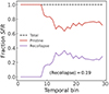 |
Fig. 1. Example of the fractional SFR contribution originating from recollapsing shells using the method discussed in Sect. 3.3. The system is assumed to have a uniform SFH and has TODDLERS parameters fixed at Z = 0.02, ϵSF = 0.025, ncl = 320 cm−3. The mean value of recollapsing shells is 19%. |
It is worth mentioning that this method could lead to negative weights in some cases. An example of this could be the case of a system exhibiting a sharply declining star formation history (SFH) in the 30 Myr period. In these cases, (ϵSF, ncl) combinations which do not exhibit recollapse could be used instead.
3.4. Older stellar population
All stellar particles with an age greater than 30 Myr are assumed to be in systems that have cleared dust and gas around them. These are assigned SEDs from the Bruzual & Charlot (2003) template library based on metallicity and age. We employ a Chabrier IMF while using this library. Table 1 summarizes the various parameters related to the input radiation sources and the dusty media, the last column states the source of the values used in the SKIRT input model.
Input parameters of the SKIRT radiative transfer model for each of the Auriga components, in addition to the particle and cell positions.
3.5. Radiative transfer configuration
The SKIRT simulations carried in this work are broadly comprised of two steps: first, the propagation of light originating from primary sources through the computational domain to assess the absorption of energy by interstellar dust; second, the propagation in the previous determines the temperature distribution, and thus, the thermal emission properties of the dust on a cell-by-cell basis within the domain. If the secondary emission is turned on, the thermal emission spectrum of each cell is propagated to generate mock observations at longer wavelengths. Given the aforementioned procedure, the fidelity of a SKIRT simulation critically depends on the optimal discretization of the computational domain. To generate optimal spatial grids for Auriga galaxies, we used an octree grid with levels of 6 to 12 and a maximum cell dust fraction value of 10−6.
Regarding the wavelength grids employed in this work, we note that SKIRT employs separate, independent wavelength grids for the sources, the mean radiation field, the dust emission, and the instruments (Camps & Baes 2020). We use a logarithmic wavelength grid with 40 points running from 0.02 μm to 10 μm for storing the mean radiation field in each cell. For dust emission, a nested logarithmic grid is employed. The low-resolution part of this nested grid has 100 points, running from 1 μm to 2000 μm, whereas the higher-resolution part runs in the polycyclic aromatic hydrocarbon (PAH) emission range from 2 μm to 25 μm with 400 wavelength points.
3.6. Calibration
Following K21, we used an SFR, stellar-mass, and morphology-based criteria to make a cut in the DustPedia sample. For the DustPedia galaxies, the SFR is the one obtained as a result of SED fitting carried out using the CIGALE code (Roehlly et al. 2012; Boquien et al. 2019). This SED fitting follows the settings described in Bianchi et al. (2018), Nersesian et al. (2019), Trčka et al. (2020). As the entire Auriga sample is star-forming at z = 0, we consider DustPedia star-forming galaxies with SFRcig > 0.8 M⊙ yr−1, where SFRcig is the SFR inferred using the CIGALE SED fitting code. The stellar mass is tracked by the flux in the 2MASS-K band, with a pivot wavelength of 2.16 μm. We note that this is different from K21, where the WISE-W1 band was used as a proxy for the stellar mass. We make this choice in order to avoid the contribution of the PAH features that contribute to this band. We chose all the DustPedia galaxies that fall within the K-band luminosity range of the Auriga sample. Finally, the DustPedia dataset is limited to late-type galaxies (Hubble stage > 0 in the DustPedia catalog). These cuts in the Dustpedia sample result in 45 galaxies, which we call DPD45 in the text.
We keep the dust-to-metal fraction for the diffuse dust fixed at the value found in K21, namely, fdust = 0.14. Keeping this value fixed ensures that a consistent comparison can be made with the results obtained in that paper, where HiiM3 was employed as the emission library for star-forming regions. On the other hand, the free parameters of the TODDLERS model (ϵSF, ncl) are found by comparing broadband luminosity scaling relations between the post-processed Auriga galaxies and DPD45. To quantify the effect of changing the free parameters, we used a two-dimensional (2D) generalization of the well-known Kolmogorov–Smirnov (K-S) test (Peacock 1983). The K-S test computes a metric D which can be interpreted as a measure of the “distance” between two sets of 2D data points, with smaller D values indicating better correspondence. The selected values of the free parameters are the ones that minimize the average D value obtained by applying the K-S test on set of scaling relations. We chose the scaling relation between 2MASS-K, and each one of GALEX-FUV, GALEX-NUV, WISE-22, SPIRE-250, and SPIRE-500 for this purpose. We note that our calibration is robust regardless of the method used to calculate the distance between DPD45 and the synthetic datasets. We confirmed this by testing with the 2D Wasserstein distance (Bonneel et al. 2015).
By scanning the TODDLERS’ parameter space, we find that the parameter set ϵSF = 0.025, ncl = 320 cm−3 gives a very good match to the observational data. We note that while the minimum of the average D is degenerate to the free parameters of the model, the chosen parameter set shows a good agreement across all the broadbands used for calibration. Figure 2 shows the scaling relations when the optimal values of the free parameters are employed. Also shown in Fig. 2 are the scaling relations obtained for the Auriga galaxies using HiiM3 star-forming regions’ library and the calibration described in K21.
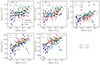 |
Fig. 2. Comparison of broad-band luminosity scaling relations between the DustPedia sub-sample DPD44 (blue stars) and SKIRT post-processed Auriga galaxies using the two available star-forming regions’ libraries in SKIRT, TODDLERS (red crosses), and HiiM3 (green crosses) at the calibrated parameter values. The Auriga sample in both cases consists of 60 points, including an edge-on and face-on configuration for each of the 30 Auriga galaxies. The rolling median lines use four bins of equal width in the K-band luminosity, LK. |
The scaling relations obtained with the calibrated TODDLERS parameter set exhibit a higher level of consistency with the observational data when compared to the HiiM3 calibrated scaling relations, as indicated by the average D value. It is especially worth mentioning the enhanced attenuation in the GALEX bands resulting from the change in the star-forming regions’ library, where the average decrease in the FUV band with respect to the runs in K21 is ≈0.3 dex. This is an encouraging development in light of the findings in previous studies of a similar nature which found higher FUV and NUV luminosities when compared to observations. These discrepancies were attributed to the star-forming regions library (e.g., Baes et al. 2019; Trčka et al. 2020, 2022; Kapoor et al. 2021; Camps et al. 2022; Gebek et al. 2024).
4. Synthetic data products
For the purpose of this work, we generated the following synthetic data products for the Auriga galaxies:
-
Broadband images were generated in the same set of 50 broadbands as those used in K21. Additionally, we generated transparent images in the UV and optical bands. To achieve this, we used the incident stellar spectra from TODDLERS models and removed the diffuse dust.
-
High spectral resolution images were generated in the wavelength range of 0.3 − 0.7 μm with a spectral resolution of R = λ/Δλ = 3000. We used SKIRT in the extinction-only mode for this set. An example of the result obtained by spatially integrating such images is shown on the left side of Fig. 3. Apart from this, we also calculate transparent images without diffuse dust and foreground dust attenuation in the TODDLERS models. However, the TODDLERS models do consider the Lyman continuum (LyC) absorption by dust. We note that the choice of the spectral resolution for the images is not limited by TODDLERS library, which was sampled at R = 5 × 10⁴. This choice is simply motivated by the computation time and the fact that we did not consider any kinematics in this work.
-
High spectral resolution images were generated in the FIR wavelength range of 10 − 200 μm. We focused on small windows within this wavelength range to generate luminosity maps of a set of fine-structure lines. The used lines and the windows are shown on the right-side panel of Fig. 3. We note that these images are the projections of light from the star-forming regions alone and do not take into account any diffuse media.
-
Projected physical property maps: These maps include 2D projections of the physical properties such as the SFR surface density averaged over a certain period, the stellar mass surface density (Σ⋆), mass-weighted metallicity, and mass-weighted stellar ages. These maps serve as the true values whenever we carried out a a comparison with synthetic observations.
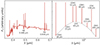 |
Fig. 3. Observables generated for the line-emission-based analysis carried out in this work. Left: Spectrum at a resolution R = 3000 in the optical 0.4 − 0.7 μm, right: Selected windows for lines in the FIR, again at R = 3000. At each of these wavelengths, we also generate images at a spatial resolution of 0.5 kpc. |
The images and the projected physical property maps were generated with a spatial resolution Δx = 500 pc/pix, and at four inclinations: 0°, 30°, 60°, and 90°. The field of view (FOV) was fixed to 90 kpc for all maps. The optimal choice of the number of photon packets for the SKIRT runs is dependent on both the spatial and spectral resolution. The choices made in this work are discussed in Appendix A.
5. UV-mm SEDs and broadband maps
In this section, we focus on the global Auriga SEDs and the broadband maps generated from our post-processing procedure. The SEDs provide a convenient way to highlight the differences arising from variations in sub-grid treatment and calibration choices. Following this, we use the broadband maps to produce maps of quantities related to the correction of dust-obscured UV. Additionally, we examine resolved maps of MIR-FIR colors and compare them to observational data.
5.1. UV–mm SEDs: TODDLERS vs. HiiM3
In Sect. 3.6 we showed that it is possible to successfully calibrate the TODDLERS parameters to reproduce observational scaling relations. In this section we consider the Auriga UV-mm SEDs and the implications of changing the of star-forming regions’ sub-grid treatment as well as varying the TODDLERS parameters around the calibrated values. Figure 4 shows the median SEDs for all the Auriga galaxies for various combinations of the two TODDLERS parameters along with the median SED obtained in K21 using the HiiM3 library. The filled area gives the range of values encountered for the entire Auriga sample. The median values and the ranges are calculated using SEDs at 0°, 90° for each of the Auriga galaxies.
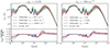 |
Fig. 4. Comparison of the median UV-mm SEDs from the SKIRT post-processed Auriga galaxies using the two available star-forming regions libraries in SKIRT, TODDLERS (red) and HiiM3 (green) at the calibrated parameter values. The median is calculated by considering only the exactly edge-on and face-on inclinations. The corresponding filled areas give the range of values encountered for the entire Auriga sample. The lower panels show the ratio of the median SED obtained using TODDLERS and HiiM3 libraries, with the range shown by the filled area only for the fiducial run. |
The left panel in Fig. 4 shows the impact of changing ncl in the range 80 − 1280 cm−3 while keeping fixed at ϵSF = 0.025, while in the right panel ϵSF is varied from 0.01 − 0.05 while keeping ncl fixed at 320 cm−3. In comparison to the HiiM3 library, with its free parameters calibrated in K21, the most significant differences are in the UV attenuation, MIR emission, and the FIR emission in the 50−100 μm spectral regimes. A comparison of the images obtained using these two libraries in selected bands is shown in Fig. C.1. The dust emission characteristics are primarily a result of the non-PAH dust size distribution in TODDLERS having a cut-off at 0.03 μm. This implies that the MIR emission contribution from non-PAH dust is only sizeable when the radiation intensity is high, namely, during the early stages of evolution. Instead, the grain size distribution leads to a stronger emission in the 50−100 μm range.
We note that the changes in UV attenuation and MIR emission, resulting from the altered sub-grid treatment of emission from star-forming regions, reduce the discrepancies with observational data reported in earlier studies of similar nature (see Sect. 3.6). Additionally, a recent comparison of IllustrisTNG-100 galaxies post-processed with HiiM3 templates has shown that these galaxies produce bluer FUV-NUV colors compared to observational data (Gebek et al. 2024). By changing the star-forming regions’ treatment to TODDLERS, this discrepancy is reduced. This can also be inferred from the redder UV slopes in the SEDs produced using TODDLERS in Fig. 4, compared to those produced with HiiM3. The better agreement with observational data is not limited to the UV and UV colors; in Sect. 5.3 we demonstrate this for the resolved MIR-FIR colors of the Auriga sample.
As for the impact of changing the two parameters of TODDLERS, increasing ncl at a fixed ϵSF leads to more compact star-forming regions. This tends to increase the UV attenuation in Auriga galaxies and a shift of the FIR peak to lower wavelengths. On the other hand, increasing ϵSF at a fixed ncl leads to a lower UV attenuation, with a slight movement of the FIR peak to lower wavelengths. It is worth noting that the attenuation in the star-forming regions also impacts the emission by the diffuse dust, which is not deficient in small grains. In particular, the single-photon heating contribution in the MIR goes up with TODDLERS parameters which promote a rapid dissolution of the clouds, namely, at lower ncl and/or higher ϵSF. Rapid shell dissolution ensures that the UV from star-forming regions escapes with a lower attenuation and heats the diffuse dust.
5.2. UV-mm broadband maps
To carry out a spatially resolved analysis on the broadband images generated by our TODDLERS-SKIRT post-processing pipeline, we used all the pixels within Ropt2, the optical radius defined in Grand et al. (2017, Table 1). We assumed the native physical resolution of our images (500 pc/pix) to be equivalent to an angular resolution of 12″. All images were then convolved with a SPIRE-500 μm point spread function (PSF) using the convolution kernels of Aniano et al. (2011). This was followed by a re-gridding procedure that generates a photometric grid across each galaxy containing individual squares 36″ × 36″ in size. These squares have a side corresponding to a physical scale of 1.5 kpc, which is comparable to the physical pixel scale of the observational data we employ for comparison. The convolution process uses astropy.convolution.convolve_fft3 and the re-gridding employs the reproject package4 with reproject_exact algorithm. We apply the aforementioned data processing method to each of the Auriga galaxies, considering three face-on inclinations: 0.0°, 30.0°, and 60.0°.
To maintain consistency with the observational datasets used in this section, we apply a selection criterion to the Auriga galaxies based on their disc-mass-fraction (fdisc). We use the values reported in Grand et al. (2017, Table 1) and select galaxies with fdisc ≥ 0.5. This criterion results in a sub-sample of 22 galaxies, which we refer to as Auriga-D. This selection process effectively removes the most irregular and bulge-dominated systems, leaving us with a disk-dominated subset.
In the following discussion, the GALEX-FUV, IRAC 8 μm, MIPS 24 μm, PACS 70 μm, PACS 100 μm, and SPIRE 500 μm bands are simply referred to as FUV, 8, 24, 70, 100, and 500 μm bands, respectively.
5.2.1. SFR using FUV and IR broadband data: Spatially varying IR correction factors
Given that star-forming regions are often dust obscured, accurately measuring SFR necessitates the tandem use of indicators which capture obscured and unobscured star formation. To that end, hybrid calibrations using FUV and IR broadband data are available in the literature, e.g., Liu et al. (2011, hereafter referred to as L11) and those in Hao et al. (2011, hereafter referred to as H11). These can be written as:
![Mathematical equation: $$ \begin{aligned} \mathrm{SFR}(\mathrm{M_{\odot }}\,\mathrm{yr}^{-1}) = C_{1}\,[L_{\rm FUV} + k_{\rm IR}\cdot L_{\rm IR}]. \end{aligned} $$](/articles/aa/full_html/2024/12/aa51207-24/aa51207-24-eq8.gif) (5)
(5)
In Eq. (5), C1 = 4.6 × 10−44 assuming a stellar IMF as given in Kroupa (2001), with a constant SFR maintained over a period of 100 Myr, and using solar metallicity stellar models from Leitherer et al. (1999). kIR depends on the IR band used for the correction. The L11 calibration using MIR gives k24 = 6.0, and the calibration in H11 with total-infrared (TIR) uses kTIR = 0.46. The quantities within the square brackets in Eq. (5) indicates the FUV luminosities that have been corrected to their intrinsic values. The luminosities in these equations are measured in units of erg s−1.
Instead of employing a fixed kIR framework, as utilized in L11 and H11, local variations in kIR were recognized in Boquien et al. (2016, hereafter referred to as B16) by making use of the SED-fitting driven spatially resolved estimation of the FUV attenuation. Their results are based on a sample of eight star-forming spiral galaxies: NGC 628, NGC 925, NGC 1097, NGC 3351, NGC 4321, NGC 4736, NGC 5055, and NGC 7793. SED fitting was done using these galaxies, primarily of Sa type or later, at a kpc resolution. The analysis in B16 ties kIR variability to specific galactic properties, such as the specific star-formation rate (sSFR), and invites a deeper investigation into the systematics affecting kIR, specifically through the lens of simulated galaxies. The test-bed provided by simulated galaxies allows for an in-depth analysis of how factors like galaxy inclination and chosen apertures influence SFR estimations without assumptions made in SED fitting, like fixed galaxy metallicity. Furthermore, the intrinsic FUV luminosity on resolved scales is readily available. Given both the attenuated and unattenuated FUV values, we could find spatially varying infrared correction factors (kIR). We solve the following equation to do so:
 (6)
(6)
where LFUV, intr., LFUV, and LIR are the intrinsic GALEX-FUV due to the stellar particles (including the unattenuated UV from star-forming regions), the observed UV as given by the synthetic maps generated by SKIRT, and the values given by the IR synthetic maps, respectively. We use 24, 70, and TIR maps for the calculation of kIR. The TIR is based on the three-band approximation given in Table 3 of Galametz et al. (2013) which used 24, 70, and 100 μm bands to get the TIR emission. This approximation performs the best based on their goodness-of-fit criteria.
Equation (6) applied to the post-processed Auriga galaxies probes the connection between the component of the radiation heating the dust largely attributable to star formation (numerator in Eq. (6)) and the dust re-emission characteristics in realistic radiative transfer settings. Figure 5 shows kIR in the case of 24 μm, 70 μm, and TIR for three Auriga galaxies, AU-1, AU-2, and AU-21 for all pixels within the Ropt. The local kIR values can vary significantly from the single values used in the literature (see Table 2) and tend to be lower in the central parts of the galaxies. The lower central values could be understood by considering Eq. (6), in which the numerator is only affected by younger stellar populations while the denominator or dust emission is affected by the presence of both young and old stars in the spatial region being probed. Thus, in the central regions of the galaxies, where older populations dominate, there is an increasing contribution of older stars to dust emission, resulting in lower values of kIR.
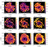 |
Fig. 5. Spatially varying IR correction factor, kIR for three Auriga galaxies in a face-on configuration. From left to right: k24, k70, and kTIR for AU-21 (top), AU-23 (middle), and AU-27 (bottom). Each panel also lists the luminosity weighted mean of the value obtained using all the pixels. |
Comparison of kIR values obtained for the Auriga-D sample and the observational sample considered in this work.
In order to readily compare the kIR values found in this work to that in the literature, we employ the light-weighted mean value, ⟨kIR⟩IR5 for each of 24 μm, 70 μm, and TIR bands. Figure 6 considers the impact of inclination and aperture on the ⟨kIR⟩IR using all the pixels from the Auriga-D sample. The aperture is reported as a fraction of Ropt, fR, opt, and uses 10 equi-spaced values between 0.25 × Ropt and Ropt. It is worth noting that the median value of Ropt for the Auriga sample is 24.25 kpc. This value is significantly higher than the FOV6 of the galaxies in B16. By visual inspection, we find that the FOV of all 8 galaxies used in that work is between 15 − 20 kpc. This range with respect to the median Auriga sample’s Ropt is represented by the gray region in Fig. 6.
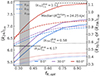 |
Fig. 6. Mean light-weighted IR correction factors, ⟨kIR⟩IR as a function of the aperture and the inclination using the galaxies in the Auriga-D sample. The aperture is given as a fraction of the optical radius, with the gray region denoting a median aperture of 15−20 kpc of the simulated galaxies. The values from B16 are shown as gray lines. |
As anticipated, due to the lower central values, enlarging the aperture size results in a consistent increase in ⟨kIR⟩IR. Similarly, increasing the inclination also leads to an increase in ⟨kIR⟩IR, because as the inclination grows, pixels receive more contributions from the outer regions of the galaxies.
Comparing to the values reported in B16, we consider two apertures fR, opt = 0.33, which corresponds to a median Auriga FOV value of ∼15 kpc which is similar to that in B16, and a larger value, fR, opt = 1. In the case of the smaller aperture, for an Auriga sample which contains all three inclination used in this work, we find that the ⟨k24⟩24 as well as the 1σ dispersion are in a very good agreement with similar quantities reported in B16. On the other hand, both ⟨k70⟩70 and ⟨kTIR⟩TIR are nearly 40% lower in the case of the smaller aperture. Although, for the same aperture, the ⟨kTIR⟩TIR value is lower by about 25% with respect to that in L11. For the larger aperture, we find that ⟨k24⟩24, ⟨k70⟩70, and ⟨kTIR⟩TIR values for the Auriga sample are around 20% higher, 25% lower, and 25% lower, respectively, in comparison to the values in B16. The ⟨kTIR⟩TIR in this case is in good agreement with the value in H11. These results are tabulated in Table 2.
5.2.2. kIR and sSFR correlations
As mentioned earlier in this paper, the numerator in Eq. (6) is related to recent star formation, while the denominator is affected by dust heating by both recent and older stellar populations. Assuming a local energy balance, we expect local variations in kIR to correlate with the sSFR, provided that the denominator can be linearly decomposed based on heating from each source. As noted by B16 (also see Draine & Li 2007), the linear decomposition of the IR contribution due to heating by old and young populations hinges on the proportionality of the IR emission in a specific band to the intensity of the incident radiation field. Notably, this applies to the TIR and the 24 μm band. The explanation is trivial in the case of the TIR. For the 24 μm and 70 μm, the correlation between incident radiation intensity and band luminosity could break down if the emission peak due grains in equilibrium passes through the band at intensity levels expected for a given application. In such cases, there is no one-to-one mapping between incident intensity and the band luminosity. This intensity threshold is high in the case of the 24 μm band emission, while it is significantly lower for the 70 μm band7.
Figure 7 presents the relation between kIR and the sSFR for the Auriga-D sub-sample using the aperture fR, opt = 1.0 at the three face-on inclinations. We reiterate that the sSFR values are calculated using the projected mass maps as discussed in Sect. 4. As expected, the Pearson correlation coefficients (PCC) for the k24 and kTIR exhibit higher values in comparison to k70. More interestingly, the values of the PCC using Auriga galaxies for k24 (0.57) and kTIR (0.73) are lower than those in B16, which have a value of 0.76 and 0.97, respectively. When using a smaller aperture, fR, opt = 0.33 for the Auriga sample, we obtain PCC values of 0.73, 0.63, and 0.74 for k24, k70, and kTIR, respectively. In the case of k24, the rise in dispersion in the k24−sSFR relation at higher sSFR values seem to be driven by the rapid change in the value of k24 for individual star-forming regions as a function of age as shown in Fig. 8. The lack of very small grains in the dust model employed in TODDLERS (lower size cut-off at 0.03 μm) means that the flux in the 24 μm band rapid declines as the shells expand (see Paper I). As for the lower kTIR, it could be an indication of the local energy balance being violated such that the IR flux is mostly heated by the stellar population outside the pixel Smith & Hayward (2018). This hypothesis could be readily tested by applying spatially resolved SED fitting to our Auriga models; however, we plan to explore this in future studies.
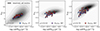 |
Fig. 7. Spatially varying IR correction factor, kIR, shown as a function of the projected sSFR for the Auriga-D sub-sample using the three face-on inclinations. The circular points represent the light-weighted values for individual galaxies at the three inclinations considered in this work. |
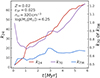 |
Fig. 8. kIR as a function of time for an individual model from the TODDLERS library. |
5.3. Resolved MIR-FIR colors of the Auriga sample
As discussed in the last section, the shape of the infrared SED is affected by the intensity of incident radiation. This fact is reflected in the color-color relations of the IR SED. Specifically, recent work carried out by Gregg et al. (2022, hereafter referred to as G22) demonstrates that galaxies with higher star-formation rate densities (SFRD) tend to show strong anti-correlations between their MIR (8/24 flux density ratios) and FIR (70/500 flux density ratios) colors. This reinforces the tight color-color relation discussed in Calzetti et al. (2018, hereafter referred to as C18), which was derived from observations of the central starburst region of the dwarf galaxy NGC 4449. Additionally, G22 note that in regions with lower SFRD, the strong MIR-FIR anti-correlation is less evident, primarily due to increased dispersion caused by heating from old stellar populations and the impact of metallicity on 8 μm emission. In general, the majority of their galaxies do not exhibit a strong MIR-FIR anti-correlation.
In the following, we describe how we used the Auriga kpc-scale broadband images and test how they stack against observational results. We have used galaxy morphology as a way to distinguish between galaxies with or without the strong anti-correlation in MIR-FIR colors. Given the large contribution in both MIR and FIR from star-forming regions, we also considered the impact of changing the sub-grid treatment on the color-color relation of Auriga galaxies.
5.3.1. Relation with morphology
Figure 9 shows the color-color relation for three Auriga galaxies, AU-1, AU-2, and AU-21, along with their SFRD maps based on the prescription in L11. These three galaxies encompass the range of MIR-FIR correlations observed in our sample. AU-1 exhibits a relatively high correlation between the blue and red colors of the IR SED, akin to the “Regime-1” galaxies described in G22, which are characterized by higher PCC. Conversely, AU-2 displays considerable dispersion in its data, mirroring the characteristics of NGC 5457 or, more broadly, the “Regime-2” galaxies in G22, characterized by the lower correlations between MIR-FIR colors. AU-21 exhibits a behaviour that is between these two. We note that the data points from the Auriga galaxies generally cluster around the relation outlined in C18, whether they exhibit significant dispersion or not.
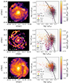 |
Fig. 9. SFRD maps (left) and associated MIR-FIR color-color relations (right) for three Auriga galaxies AU-1, AU-2, and AU-21 post-processed with TODDLERS models. The figures in the right column also indicate the PCC value, the SFR of the galaxy inferred using the calibration given in L11 (black value; see Sect. 5.2.1), and the true SFR of the galaxies averaged over 100 Myr (red value). The gray filled contours represent the colors of the KINGFISH sample as reported by G22 while the dashed curve is the relation for NGC-4449 given in C22. |
As noted in G22, the dispersion in the color-color plot largely comes down to the presence of different environments in the same galaxy. Such a difference could be either due to the presence of regions of low SFRD or to a variation in metallicity. This implies that the galaxy morphology could be a predictor of the dispersion in this color-color plane. In order to tie the dispersion in the color-color plot to the morphology of the galaxies, we used statmorph (Rodriguez-Gomez et al. 2019) on the kpc resolution SFRD maps. We used three non-parametric indicators of galaxy morphology (NPIGM) here: concentration, smoothness, and M20, which gauge the central concentration, clumpiness, and the presence of non central bright features in a galaxy, respectively. We note that a higher value of smoothness implies higher clumpiness in the image.
In order to quantify the dispersion on the color-color plot, we use the mean distance of the points from the color-color relation given in C18, namely, the black dashed curve in Fig. 9, denoted by ⟨DC18⟩. Figure 10 shows ⟨DC18⟩ as a function of the three NPIGM for all Auriga galaxies except AU-11, which is undergoing a merger. The points are color-coded by the PCC value obtained for a given galaxy. All three face-on inclinations of the Auriga galaxies have been used to populate Fig. 10.
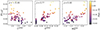 |
Fig. 10. Dispersion in Auriga galaxies’ MIR-FIR color-color plot as a function of the non-parametric indicators of galaxy morphology applied to the SFRD maps. The data includes all the three inclinations and all Auriga galaxies except AU-11, which is undergoing a merger. The data-points are color-coded using the Pearson correlation coefficient obtained for the color-color relation for individual galaxies. |
Based on Fig. 9, galaxies with lower central concentration, higher clumpiness, presence of prominent spiral arms show a higher dispersion, and thus, a lower PCC in the Auriga sample. The smoothness indicator appears to be the best in predicting the dispersion in the MIR-FIR color-color relation at kpc resolutions. This is expected and is in line with the findings in G22 due to the fact that the clumpier systems appear so due to the presence of low and high SFRD regions within the same galaxy. Galaxies with low clumpiness are more uniform in their SFRD maps, and show higher PCC. We note that more compact Auriga galaxies, like AU-10, AU-13, AU-22, AU-26, AU-28, AU-30 exhibit lower dispersion values due their high SFRD.
5.3.2. MIR-FIR colors of the Auriga sample: TODDLERS vs. HiiM3
In Paper I, we examined the MIR-FIR color–color plot employing the a population of TODDLERS star-forming regions. That comparison highlights the difference between TODDLERS and HiiM3 libraries in the observational space without considering the effects of the dust exterior to the star-forming regions, which can have a significant effect on the luminosity in the considered bands, particularly in the 8 μm and 500 μm bands. Here, we extend that comparison between TODDLERS and HiiM3 using Auriga galaxies on a kpc scale. This allows us to visualize the impact of changing the sub-grid treatment from TODDLERS to HiiM3 on the color-color plane and compare the results with the observational data from G22.
Figure 11 shows the effect of changing the sub-grid treatment of star-forming regions using the Auriga-D sub-sample using the three face-on inclinations. We note that the addition of diffuse dust to the galaxies significantly lowers the 70/500 color (cf. Fig. 21 in Paper I). The colors obtained for the Auriga galaxies using TODDLERS are largely consistent with those G22. In contrast, the results for the Auriga galaxies when using HiiM3 show an offset with respect to the observational data in both 8/24 and 70/500 colors. This is because the HiiM3 templates exhibit higher 24 μm and lower 70 μm luminosities compared to those in the TODDLERS library, using the free parameter values determined by the calibration in K21 (cf. Fig. 4).
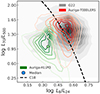 |
Fig. 11. MIR-FIR color-color diagram considering all the pixels of the Auriga-D galaxies at inclinations 0°, 30°, and 60° along with consolidated “Regime-1” and “Regime-2” data from G22 (gray region). The orange contours represent the data when TODDLERS library is employed, while the green contours are obtained in the case of HiiM3. The darkness of the contour colors represents the density of the pixels on a linear scale. Also shown are the median values for each of the three datasets using round markers of corresponding colors. The dashed black curve is the relation obtained in C18. |
6. Line-emission based SFR
Next, we used our synthetic line-emission maps to generate SFR maps. We applied two strategies, one using the Hα emission and the other using the FIR forbidden lines, [O I] 63 μm, [O III] 88 μm, and [C II] 158 μm. We re-gridded all the line-maps used in the upcoming sections to a 1 kpc resolution using the reproject_exact algorithm. We note that in order to avoid noisy pixels, we only make use of the pixels at or above the 5σ level.
6.1. SFR from Hα emission
In this section, we concentrate on deriving the SFR from Balmer line maps. Having access to both attenuated and transparent maps allows us to calculate a fitting function for the attenuation curve of the Hα line emission in Auriga galaxies as a function of the attenuation on resolved scales. We then apply a Balmer decrement-based dust correction to these maps. Additionally, we compare our results with those using 3D radiation-hydrodynamics simulations as reported in Tacchella et al. (2022, hereafter referred to as T22)
Before delving into the Balmer line maps using the Auriga galaxies at z = 0, it is worthwhile to look at the predictions from the TODDLERS models, especially at the escape fractions and the LyC destruction due to dust.
6.1.1. LyC destruction by dust and escape fractions
As discussed in Paper I, we only employ a mass-based stopping criterion in our Cloudy models, namely, the extent of our models is only dictated by mass, which makes them susceptible to leaking ionizing photons if the shells are rapidly thinned. Apart from this, TODDLERS models consider the presence of dust within H II regions which leads to the destruction of ionizing photons. In both these cases, the amount of ionizing photons that would otherwise lead to the production of Hα is reduced.
In order to quantify these effects, we generate a population of star-forming regions with uniform sampled ages between 0−30 Myr and applying the methodology discussed in Sect. 3.3 to ensure an SFR of 1 M⊙ yr−1. For this population, we calculate a Hydrogen ionizing photon rate weighted mean escape fraction, using the incident and output spectra of our models in the energy range 1.0 − 1.8 × Eion.,H, where Eion.,H is the Hydrogen ionizing energy. This averaged quantity, ⟨fesc.⟩, is shown with the dashed lines in Fig. 12. We similarly define a mean dust absorption fraction, ⟨fabs⟩. This is calculated in a manner described in Paper I. The results for Z = 0.08, 0.02, 0.04 are shown in the top row of Fig. 12.
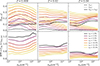 |
Fig. 12. Fraction of LyC photons that do not participate in the production of Hα at Z = 0.008, 0.02, 0.04 (top) for a population of H II regions generated (as per Sect. 3.3) for the parameters of the TODDLERS models, ϵSF and ncl. The solid line represents the sum of the escape fraction (dashed) and absorption by dust (dotted). Conversion of Hα luminosity to SFR (bottom), using a fixed conversion factor, CHα = 5.5 × 1042, using the same SF region populations and TODDLERS model parameters as the top row. |
For a population of star-forming regions such as the ones considered here, at the lowest end of the cloud density values, the presence of leaky H II regions can lead to up to ≈30% of the LyC photons escaping the system at Z = 0.02. This number declines with increasing ncl and decreasing ϵSF. The escape fractions at fixed parameter (ncl, ϵSF) generally tend to be lower (higher) at higher (lower) metallicity values shown in Fig. 12. The escape fractions from the H II regions are in good agreement with observational studies, such as Crocker et al. (2011), Pellegrini et al. (2012), and Relaño et al. (2012). We also note that these model escape fractions do not reflect galaxy escape fractions. The photons from leaky H II regions are expected to be absorbed elsewhere in the ISM and the global escape fraction are not expected to be more than a few percent Heckman et al. (2011). In the current work, we do not model the diffuse gas ionized outside the star-forming regions.
The average fraction of LyC photons absorbed by dust remains between 10 − 25%, and this fraction gradually increases with ncl and ϵSF. This is in good agreement with the values reported in literature Calzetti (2013). On the other hand, based on the radiation-hydrodynamical simulations, T22 report an ⟨fabs⟩ of 28% for a Milky-Way like simulation, closer to the higher end of the values encountered in our models. We note that the individual H II region’s fabs is correlated with the ionization parameter Paper I, thus, for a population, the averaged value would depend on the SFH. For the population considered here, the variation in the absorbed fraction of LyC photons ⟨fabs⟩ across the three metallicities, while keeping other parameters constant, is within 10%.
The bottom row of Fig. 12 shows the estimated SFR using the Hα conversion factor for Z = 0.02 and an IMF suitable for our models (CHα = 5.5 × 10−42 for Hα luminosity in erg s−1). Figure 13 shows the ratio of the SFR inferred by summing all pixels in the transparent Hα map to the simulation value averaged over the past 30 Myr employing the calibrated TODDLERS’ parameters. The scatter points’ color reflects the SFR weighted metallicity of the Auriga galaxies. It is worth noting that all Auriga galaxies exhibit an SFR weighted mean metallicity lying between 0.03 and 0.06. Using the same CHα as above results in inferred to simulation ratio values that lie in the range of 0.725−0.9.
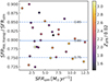 |
Fig. 13. Ratio of the inferred SFR, using a conversion factor of CHα = 5.5 × 1042, applied to the transparent Hα luminosity, compared to the SFR reported by the simulation across the entire Auriga galaxy sample. The color-coding indicates the SFR-weighted metallicity of each Auriga galaxy. |
6.1.2. Dust attenuation
The wavelength of the Hα line makes it highly susceptible to dust attenuation. Dust attenuation is dealt with using the Balmer decrement correction method, where the theoretical recombination ratio of Hα and Hβ line luminosities is known, and any changes to this value are considered to arise from the effects of dust (Osterbrock & Ferland 2006). The Balmer decrement could be summarized using the following equation:
 (7)
(7)
where, AHα is the Hα line attenuation. (Hα/Hβ)obs, (Hα/Hβ)int are the observed and intrinsic Balmer decrements, respectively. k(Hα) and k(Hβ) represent the extinction curve values for the wavelengths of Hα and Hβ, respectively. The intrinsic Balmer is typically assumed to be 2.87, a Case-B value which holds at an electron temperature of 104 K and an electron density of 100 cm−3Osterbrock & Ferland (2006). While this ratio can vary if the temperature or density change, this ratio falls in the narrow range of 2.87 − 3.05 for a wide variety of conditions, thus for the rest of this work, we used a value of 2.87 for this quantity.
Similar to the approach in T22, given that we have access to both the dust attenuated and transparent Hα maps, and thus, AHα, we invert Eq. (7) to find the attenuation law, or the ratio, k(λHα)/k(λHβ), as a function of AHα. An example of this process is given in Fig. 14, portraying the intrinsic and attenuated maps required for the calculation of AHα, and the observed Balmer decrement. Knowing these quantities and the intrinsic Balmer decrement allow us to calculate k(λHα)/k(λHβ) as a function of AHα, which is shown in the last column of that figure. At this point, it is worth pointing out that our sub-grid models for the Balmer lines, generated using Cloudy, assume isotropic transmission through dusty clouds. Consequently, the lines are subject to dust attenuation as described by the exponential integral function E2(τd) where τd represents the dust optical depth (refer to Röllig et al. 2007, for more details on the radiative transfer in Cloudy). This assumption results in a significantly enhanced intensity decay compared to the exponential decay observed at the same optical depth.
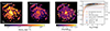 |
Fig. 14. Hα maps and attenuation law for one of the Auriga galaxies, AU-1. Panel 1: Transparent Hα surface density, Panel 2: Observed Hα surface density, Panel 3: The observed Balmer decrement, and Panel 4: The attenuation law found by inverting Eq. (7), also shown is the fit to the attenuation law for a simulated Milky-Way galaxy done in T22 (orange) and the fit to the resolved face-on data obtained in this work. |
Following T22, we assume a power-law form of the extinction curve, k ∝ λn, and fit the attenuation law using the face-on resolved data by using:
 (8)
(8)
where a, b, and c are the fitting parameters. The fit to the resolved data from 30 Auriga galaxies is shown in Fig. 15, with a = −0.187, b = 0.183, and c = −0.096. Additionally, the integrated/global values for the Auriga galaxies are shown as scatter points. The global values follow the fit to the resolved data without any dependence on the inclination. We note that as our modelling does not consider the diffuse Hα emission, it misses the lower attenuation data, which results in our fit being lower at AHα < 1 in comparison to the fit in T22.
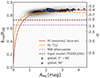 |
Fig. 15. Attenuation law obtained by using the Face-on (0° inclination) resolved data for the entire Auriga sample. The circular markers represent the integrated values for Auriga galaxies. The red curve indicates the fit to the data described in Sect. 6.1.2 while the orange curve is the fit from T22. Also shown are the Milky-Way attenuation (purple dashed line) and the input dust model value employed in TODDLERS models (maroon dashed line). |
The median value of kHα/kHβ, which defines the slope of the attenuation law, using the integrated AHα of the Auriga galaxies at all inclinations, as obtained from the resolved attenuation law fit, is 0.88. This is slightly higher than the value of 0.83 reported for simulations resembling the Milky-Way in T22. This difference is likely due to the larger median size of the dust grains employed in the TODDLERS model, which is expected to move the attenuation law to shallower slope, (see Fig. 11 in Salim & Narayanan 2020). Our fit in Fig. 15 lies slightly above the one from T22 for pixels with AHα > 2 for the same reason.
The corrected Hα to the transparent Hα ratio as a function of the observed Hα using the median kHα/kHβ value of 0.88 is shown in Fig. 16. Using this attenuation law recovers the global Hα luminosities within ±0.25 dex. Using the same attenuation law for the resolved data results in a median overestimation of 0.14 dex. This is expected given the dependence of Balmer decrement correction on resolution (Vale Asari et al. 2020).
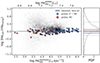 |
Fig. 16. Balmer-decrement based attenuation correction for our models when applied to Auriga galaxies as described in Sect. 6.1.2. The ratio of corrected Hα to transparent Hα is shown as a function of the observed Hα luminosity. The circular markers represent the global values while the hexbins represent the kpc-scale data. |
6.2. SFR from FIR lines
In the relatively cooler regions of the ISM, such as in photo-dissociation regions (PDRs), the emission of far-infrared forbidden lines of elements such as carbon and oxygen facilitates cooling. The first ionization energy of oxygen is 13.62 eV, which closely matches that of hydrogen. Therefore, in regions of the ISM where Hydrogen is neutral, oxygen is also predominantly O I. In contrast, carbon largely exists as the singly ionized C II due to its lower first ionization energy of 11.3 eV. This is low enough that the Milky Way’s ultraviolet radiation field can maintain the neutral carbon fraction as low as 10−3 (Ryden & Pogge 2021). Given the difference of energies of transition (Eu in Table B.1), [C II] 158 μm ([C II] from here onwards) dominates cooling under 100 K in neutral regions, while [O I] 63 μm ([O I] from here onwards) plays an important role in the 500 ≤ T [K]≤8000 neutral regime. Considering Table B.1, [O III] 88 μm line ([O III] from here onwards), with an upper state energy of approximately 163 K and a high ionization potential of 35.1 eV for O+, emerges primarily from diffuse, highly ionized regions near young O stars. However, due to its low critical density for excitation, other lines, such as [O III] 52 μm and optical lines including [O III] 5007 Å and Hα, might play dominant roles in the cooling of ionized gas regions at higher densities.
The use of [C II] 158 μm as an SFR indicator is directly related to its action as the principal coolant for the neutral atomic gas in the interstellar medium. Consequently, its high luminosity makes it attractive as an indicator for distant galaxies. However, the limitations in terms of density (both electron and hydrogen) in ionized and neutral regimes, respectively, means that [C II] line may not effectively trace dense neutral gas that is poised for imminent star formation, or ionized gas around young stars. [O I] serves as an effective coolant in dense and/or warm PDRs. This connection to PDRs links it to star-forming activities. This is also a luminous line, generally observed to be the second brightest line following [C II] 158 μm. The [O III] line is directly linked to star formation as this line primarily emanates from diffuse, highly ionized regions around young O stars, offering insights into the early stages of star formation, but as mentioned earlier, its low electron critical density could lead to lower brightness.
The TODDLERS library offers support for all of these lines, with the important caveat that these lines only emerge from gas around young stars. It is also worth noting that the results are an aggregate of all star-forming regions, thus, no inclination effects are present. Future releases of SKIRT will allow users to add contributions of the diffuse media to these lines, it is a worthwhile effort to see the contribution of star-forming regions alone.
6.2.1. Global SFR comparison
To compare the global SFR values of Auriga galaxies with those in the literature, we reference results from De Looze et al. (2011, 2014b) and Herrera-Camus et al. (2015) (hereafter referred to as DL11, DL14, and HC15, respectively) for the [C II] line. For the [O I] and [O III] lines, we used results from De Looze et al. (2014b). The L11 sample consists of 24 local star-forming galaxies given in Brauher et al. (2008). We used the SFR calibration for the nearby metal poor dwarfs and starburst galaxies reported in DL14 (see Table 3 in that paper). The HC15 sample comprises 46 local star-forming galaxies selected from the KINGFISH catalog (Kennicutt et al. 2011). The calibration is given as:
![Mathematical equation: $$ \begin{aligned} \log (\mathrm{SFR}[\mathrm{M_{\odot }\,yr^{-1}}]) = \alpha + \beta \,\log (L_{\mathrm{line}}[\mathrm{L_{\odot }}]), \end{aligned} $$](/articles/aa/full_html/2024/12/aa51207-24/aa51207-24-eq12.gif) (9)
(9)
with the fitting coefficients for the various observational datasets employed for comparison with our data given in Table 3.
Fitting function coefficients and dispersion for the global observational data used in this work.
Figure 17 shows the simulations’ true SFR averaged over 30 Myr as a function of line luminosity obtained with our post-processing procedure. The L−SFR relation is shown for two apertures for the Auriga galaxies. Also shown are the reference literature SFR calibrations from DL11, DL14, and HC15. The 1σ scatter is shown as filled regions. The L−SFR for the Auriga galaxies using the [C II] line is in good agreement with the observational data. The effect of aperture does not change the slope of the relation.
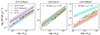 |
Fig. 17. Line luminosity vs. SFR relation for the Auriga galaxies post-processed with the TODDLERS library. The SFR for the Auriga galaxies is the simulation reported value averaged over 30 Myr. The orange points represent values using an aperture (see Sect. 5.2.1) fR, opt = 1, while the green ones are for fR, opt = 0.33. The straight lines represent various observational relations and the associated filled areas represent the 1σ dispersion on the calibration. |
As for the L−SFR relation for [O I] line, while the Auriga galaxies’ are largely within the observational scatter, they appear to have somewhat higher [O I] line luminosities in comparison to the observed galaxies of similar SFR values. This is likely due to a higher metallicity of our star-forming regions. We expect the self-absorption effects to add additional dispersion in the relation due to inclination effects. The effect of a change in aperture does not lead to a large systematic change in the L−SFR relation of the Auriga galaxies.
In the case of the [O III] line, the literature calibrations for the dwarf and starburst galaxies show a very large difference. This is expected given the low critical density of the [O III] line. The Auriga L−SFR relation is sandwiched between the relations for the two different galaxy kinds. We also note that the starburst sample in DL14 just contains 9 galaxies. The L−SFR relation for the smaller aperture shows a systematic offset with respect to the larger one, this is likely an effect of the metallicity gradient in the galaxies. The central parts of the galaxies have a higher metallicity, thus a lower ionizing photon production. Also, the higher mechanical luminosity associated with clusters of higher metallicity leads to shells at higher gas densities.
6.2.2. Resolved SFR comparison
We employ synthetic maps for the [C II], [O I], and [O III] lines and compare them with the true projected values to create fitting functions for the Auriga galaxies. We fit a straight line in log-log space using the kpc-scale maps of the three fine-structure line maps from all 30 Auriga galaxies. This allows us to determine the values of α and β for the equation of the form:
![Mathematical equation: $$ \begin{aligned} \log (\Sigma _{\mathrm{SFR} }[\mathrm{M_{\odot }\,yr^{-1}\,kpc^{-2}}]) = \alpha + \beta \,\log (\Sigma _{\rm line}[\mathrm{L_{\odot }\,kpc^{-2}}]). \end{aligned} $$](/articles/aa/full_html/2024/12/aa51207-24/aa51207-24-eq13.gif) (10)
(10)
The results of this fitting procedure are are shown in Fig. 18. Also shown are the Σline − ΣSFR relations for the low-metallicity dwarf galaxies from DL14. In the case of [C II] line, the relation in HC15 is also shown (see Table 4). These relations are given below:
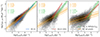 |
Fig. 18. Linear fits in the log-log space obtained using the line-emission for Auriga galaxies based on Eq. (10). The shaded area signifies the 1σ dispersion of the fits. The orange fits uses all the pixels, while the green ones only use the brightest 10% of pixels out of the entire Auriga sample for each line. The observational fits for metal-poor dwarf galaxies reported in DL14 are shown in red while those for the [C II] line reported in HC15 are shown in blue. The filled areas represent the 1σ dispersion on the various fits. |
Fitting function coefficients and dispersion for the resolved observational data used in this work.
We calculated two kinds of fits for the Auriga galaxies: 1. a fit using all pixels with a brightness level at and above 5σ level. 2. a fit using pixels above the 90 percentile level, namely, the brightest 10% pixels. Considering the slope of the fits arising from the use of all pixels in the Auriga sample, Auriga galaxies’ [C II] fits are sub-linear, both DL14 and HC15 report higher values of the slope. Given that we are missing a [C II] producing component, it is non-trivial to speculate how its presence would influence this relation. We plan to redo this comparison with a more comprehensive ISM model in future. Interestingly, the ![Mathematical equation: $ \Sigma_{[{\mathrm{C}\,\textsc{ii}}]}{-}\Sigma_{\mathrm{SFR}} $](/articles/aa/full_html/2024/12/aa51207-24/aa51207-24-eq14.gif) relation for the brightest 10% of the pixels agrees quite well with the relation given in HC15 as well as DL14.
relation for the brightest 10% of the pixels agrees quite well with the relation given in HC15 as well as DL14.
For ![Mathematical equation: $ \Sigma_{[{\mathrm{O}\,\textsc{i}}]}{-}\Sigma_{\mathrm{SFR}} $](/articles/aa/full_html/2024/12/aa51207-24/aa51207-24-eq15.gif) and
and ![Mathematical equation: $ \Sigma_{[{\mathrm{O}\,\textsc{iii}}]}{-}\Sigma_{\mathrm{SFR}} $](/articles/aa/full_html/2024/12/aa51207-24/aa51207-24-eq16.gif) , we find increasing flatter overall relations, only for the most luminous parts of the Auriga galaxies these relations show a super-linear relation. The dispersion in the relation is also higher for the [O I] and [O III] lines in comparison to that of the [C II] relation with the [O III] line’s relation showing the highest dispersion. Remarkably, the slopes of the [O I] and [O III] lines’ relations of the brightest Auriga pixels show similar slopes as those obtained for the low-metallicity dwarf galaxies in DL14.
, we find increasing flatter overall relations, only for the most luminous parts of the Auriga galaxies these relations show a super-linear relation. The dispersion in the relation is also higher for the [O I] and [O III] lines in comparison to that of the [C II] relation with the [O III] line’s relation showing the highest dispersion. Remarkably, the slopes of the [O I] and [O III] lines’ relations of the brightest Auriga pixels show similar slopes as those obtained for the low-metallicity dwarf galaxies in DL14.
7. Summary and outlook
In this study, we use the TODDLERS emission library for star-forming regions within SKIRT radiative transfer code to produce several synthetic observations for the 30 Milky Way-like galaxies of the Auriga simulation suite. We have updated the population synthesis method using the TODDLERS library in order to match the SFR of the simulated galaxies while considering the SFR contribution due to recollapsing shells. The calibration of the model parameters follows a method similar to Kapoor et al. (2021). This involves using analogous galaxies from the DustPedia project and comparing the multi-wavelength broadband data of the simulated galaxies with that of the observed galaxies. The calibrated Auriga broadband data shows higher level of agreement with the DustPedia galaxies, particularly in the UV and MIR bands compared to the data in Kapoor et al. (2021).
We have produced publicly available broadband and line-emission maps at a spatial resolution of 0.5 kpc. The broadband maps consist of 50 commonly used filters spanning the UV-mm range. We have calculated two kinds of line-emission maps: 1. a set of maps in the optical wavelength range of 0.3 − 0.7 μm, 2. a set of maps with specific spectral windows centered at the wavelengths of bright IR lines. These lines are [S III] 18 μm, [S III] 33 μm, [O III] 52 μm, [O I] 63 μm, [O III] 88 μm, [N II] 122 μm, [C II] 158 μm, and [N II] 205 μm. Both these have a spectral resolution, R = 3000. The following summarizes the main results and conclusions of this work:
-
Using the integrated Auriga UV-mm SEDs, we find that the TODDLERS based star-forming regions’ treatment allows for higher FUV and NUV attenuation, and lower MIR emission around 24 μm relative to the SEDs obtained for Auriga galaxies using HiiM3. Earlier studies have consistently pointed out issues with these exact wavelength regimes (e.g., Baes et al. 2019; Trčka et al. 2020, 2022; Kapoor et al. 2021; Camps et al. 2022; Gebek et al. 2024), with SEDs produced with HiiM3 exhibiting lower UV attenuation and higher MIR fluxes. Additionally, TODDLERS produces stronger FIR emission in the 50−100 μm range, influenced by the non-PAH dust size distribution, which has a lower cut-off at 0.03 μm.
-
We performed a self-consistent calculation of the IR correction factors used for SFR calculation using observed FUV and IR data. This is calculated as:
 . The IR bands utilized for this calculation are 24 μm, 70 μm, and TIR. The kIR values vary significantly across different regions of a galaxy and are influenced by sSFR as dust heating is from both young and old stellar populations. Enlarging the aperture size and increasing galaxy inclination generally increases light-weighted mean kIR values. The kIR−sSFR correlations observed in our study were somewhat lower than those reported in Boquien et al. (2016), where the authors employed SED fitting to derive the values. In particular, the lower Pearson correlation coefficient in the case of kTIR−sSFR seems to suggest that the local energy balance employed in the SED fitting needs a critical examination. We plan to do this in a future work using our post-processed galaxies and the CIGALE code.
 -
Our models show that galaxies with higher SFR densities exhibit strong anti-correlations between their MIR and FIR colors, aligning with observational findings in Calzetti et al. (2018), Gregg et al. (2022). At the same time, the dispersion in MIR-FIR color-color plots is influenced by galaxy morphology, with clumpier systems (higher smoothness values) showing greater dispersion. The presence of low and high SFRD regions within galaxies tends to increase the dispersion through the variations in 8 μm emission. It is also noteworthy that the MIR-FIR colors of the Auriga galaxies using the TODDLERS sub-grid treatment were largely consistent with local galaxy data from Gregg et al. (2022). In contrast, the HiiM3 templates show significant offsets.
-
Using the TODDLERS library, we quantify the reduction in ionizing photons available for Hα production due to 1. dust within H II regions, and 2. the escape fractions. For a population of H II regions with a constant SFR and Z ∈ [0.008, 0.02, 0.04], 10−25% of LyC photons are absorbed by dust, consistent with existing literature. The escape fraction of LyC photons varies with ncl and ϵSF, with up to 30% escaping, decreasing as ncl increases and ϵSF decreases.
-
We have calculated an attenuation law (kHα/kHβ) for Hα based on the dust-attenuated and transparent Hα maps. For the kpc-resolved Auriga data, the attenuation law is generally a function of the Hα attenuation. We determined a fitting function for the attenuation law as a function of the Hα attenuation. The median value of the attenuation law using the global AHα and the fitting function is found to be 0.88, which is slightly higher than that reported by the radiation hydrodynamical simulations of Tacchella et al. (2022). This discrepancy is likely due to the larger median size of dust grains in the TODDLERS models. Applying this attenuation law in the Balmer decrement correction equation corrects the observed global Hα luminosities to within ±0.25 dex of the transparent values.
-
Using FIR fine-structure lines [C II] 158 μm, [O I] 63 μm, and [O III] 88 μm originating from gas in star-forming regions, we compare the results with those in De Looze et al. (2011, 2014b), Herrera-Camus et al. (2015). On a global scale, we find a good agreement between the Auriga models and the observational L−SFR relation for the [C II] line. In the case of [O I], the Auriga galaxies exhibit somewhat higher line luminosities at a given SFR compared to results in De Looze et al. (2014b), we attribute this to the higher metallicity of the Auriga SF regions. The observational [O III] SFR calibration is highly dependent on the galaxy type given the lower critical density of the [O III] line. We find that the Auriga [O III] L−SFR relation lies between the starburst and the metal poor dwarf galaxy sample of De Looze et al. (2014b). Additionally, we employed synthetic kpc-resolved maps for the [C II], [O I], and [O III] FIR lines and projected SFRD maps to calculate log-log space linear fitting functions for the Auriga galaxies’ line brightness and SFRD. Our fits have sub-linear slopes for all three lines when using all the Auriga pixels, but super-linear slopes when using only the brightest 10% pixels.
This work is the first study to use the TODDLERS library for post-processing hydrodynamical simulations. The next step is to use the TODDLERS library to produce high spatial and spectral resolution IFU cubes for a broader array of galaxies (Andreadis et al., in prep.). This effort will utilize SKIRT’s comprehensive support for gas and stellar kinematics. Additionally, we are developing a more detailed ISM model within SKIRT to include emission from diffuse gas. Applying the post-processing methods described in this study to various redshift snapshots will also allow us to directly explore and assess the cosmic evolution of galaxy morphology and various scaling relations. Applying the TODDLERS framework to a broader range of galaxies and across various redshifts will provide valuable insights that can be used to refine the model. In the future, we aim to enhance the model’s versatility by adjusting the stellar templates to reflect different abundance sets, the specific physical processes at play, and variations in the IMF. Additionally, we plan to adapt the dust model within TODDLERS to better represent the diverse conditions found in different galactic environments. These modifications will help improve the model’s predictions and extend its applicability across a wider range of scenarios.
8. Data availability
All the synthetic observations generated for this work are publicly available at www.auriga.ugent.be. The cosmological simulation data from the Auriga Project used in this work are publicly available at https://wwwmpa.mpa-garching.mpg.de/auriga/data
105 − 106.75 M⊙ in steps of 0.25 dex.
2 × Ropt is always smaller than the original FOV of 90 kpc used for our maps.
In contrast, the mean kIR is represented simply by ⟨kIR⟩.
FOV is assumed to be twice the radius of the circular aperture.
Typical values for Draine & Li (2007, Fig. 15 in that work) model are ∼105 U and ∼50 U, respectively, where U is the interstellar radiation field in the solar neighborhood.
Acknowledgments
We thank Remy Indebetouw, Ilse De Looze, Jérémy Chastenet, and Brian Van Den Noortgaete for useful discussions. We thank Benjamin Gregg for providing the MIR-FIR colors’ data from the KINGFISH sample. Additionally, we would like to express our gratitude to the anonymous referee for their valuable feedback. MaBa and AG acknowledge the financial support of the Flemish Fund for Scientific Research (FWO-Vlaanderen). MéBo gratefully acknowledges support from the ANID BASAL project FB210003 and from the FONDECYT regular grant 1211000. This work was supported by the French government through the France 2030 investment plan managed by the National Research Agency (ANR), as part of the Initiative of Excellence of Université Côte d’Azur under reference number ANR-15-IDEX-01. The simulations carried out for this work used the Tier-2 facilities of the Flemish Supercomputer Center (https://www.vscentrum.be) located at Ghent University.
References
- Aniano, G., Draine, B. T., Gordon, K. D., & Sandstrom, K. 2011, PASP, 123, 1218 [Google Scholar]
- Bacon, R., Accardo, M., Adjali, L., et al. 2010, SPIE Conf. Ser., 7735, 773508 [Google Scholar]
- Baes, M., & Camps, P. 2015, Astron. Comput., 12, 33 [NASA ADS] [CrossRef] [Google Scholar]
- Baes, M., Verstappen, J., De Looze, I., et al. 2011, ApJS, 196, 22 [Google Scholar]
- Baes, M., Trčka, A., Camps, P., et al. 2019, MNRAS, 484, 4069 [Google Scholar]
- Baes, M., Gebek, A., Trčka, A., et al. 2024, A&A, 683, A181 [NASA ADS] [CrossRef] [EDP Sciences] [Google Scholar]
- Barrientos Acevedo, D., van der Wel, A., Baes, M., et al. 2023, MNRAS, 524, 907 [NASA ADS] [CrossRef] [Google Scholar]
- Benítez-Llambay, A., Navarro, J. F., Frenk, C. S., & Ludlow, A. D. 2018, MNRAS, 473, 1019 [CrossRef] [Google Scholar]
- Bianchi, S., De Vis, P., Viaene, S., et al. 2018, A&A, 620, A112 [NASA ADS] [CrossRef] [EDP Sciences] [Google Scholar]
- Björklund, R., Sundqvist, J. O., Singh, S. M., Puls, J., & Najarro, F. 2023, A&A, 676, A109 [NASA ADS] [CrossRef] [EDP Sciences] [Google Scholar]
- Bonneel, N., Rabin, J., Peyré, G., & Pfister, H. 2015, J. Math. Imaging Vision, 51, 22 [NASA ADS] [CrossRef] [Google Scholar]
- Boquien, M., Kennicutt, R., Calzetti, D., et al. 2016, A&A, 591, A6 [NASA ADS] [CrossRef] [EDP Sciences] [Google Scholar]
- Boquien, M., Burgarella, D., Roehlly, Y., et al. 2019, A&A, 622, A103 [NASA ADS] [CrossRef] [EDP Sciences] [Google Scholar]
- Brauher, J. R., Dale, D. A., & Helou, G. 2008, ApJS, 178, 280 [NASA ADS] [CrossRef] [Google Scholar]
- Bruzual, G., & Charlot, S. 2003, MNRAS, 344, 1000 [NASA ADS] [CrossRef] [Google Scholar]
- Calzetti, D. 2013, in Secular Evolution of Galaxies, eds. J. Falcón-Barroso, & J. H. Knapen (IOP Science), 419 [CrossRef] [Google Scholar]
- Calzetti, D., Armus, L., Bohlin, R. C., et al. 2000, ApJ, 533, 682 [NASA ADS] [CrossRef] [Google Scholar]
- Calzetti, D., Wilson, G. W., Draine, B. T., et al. 2018, ApJ, 852, 106 [NASA ADS] [CrossRef] [Google Scholar]
- Camps, P., & Baes, M. 2015, Astron. Comput., 9, 20 [Google Scholar]
- Camps, P., & Baes, M. 2020, Astron. Comput., 31, 100381 [NASA ADS] [CrossRef] [Google Scholar]
- Camps, P., Baes, M., & Saftly, W. 2013, A&A, 560, A35 [NASA ADS] [CrossRef] [EDP Sciences] [Google Scholar]
- Camps, P., Misselt, K., Bianchi, S., et al. 2015, A&A, 580, A87 [NASA ADS] [CrossRef] [EDP Sciences] [Google Scholar]
- Camps, P., Trayford, J. W., Baes, M., et al. 2016, MNRAS, 462, 1057 [CrossRef] [Google Scholar]
- Camps, P., Behrens, C., Baes, M., Kapoor, A. U., & Grand, R. 2021, ApJ, 916, 39 [NASA ADS] [CrossRef] [Google Scholar]
- Camps, P., Kapoor, A. U., Trcka, A., et al. 2022, MNRAS, 512, 2728 [NASA ADS] [CrossRef] [Google Scholar]
- Casasola, V., Cassarà, L. P., Bianchi, S., et al. 2017, A&A, 605, A18 [NASA ADS] [CrossRef] [EDP Sciences] [Google Scholar]
- Casasola, V., Bianchi, S., De Vis, P., et al. 2020, A&A, 633, A100 [NASA ADS] [CrossRef] [EDP Sciences] [Google Scholar]
- Casasola, V., Bianchi, S., Magrini, L., et al. 2022, A&A, 668, A130 [NASA ADS] [CrossRef] [EDP Sciences] [Google Scholar]
- Chabrier, G. 2003, PASP, 115, 763 [Google Scholar]
- Chaikin, E., Schaye, J., Schaller, M., et al. 2023, MNRAS, 523, 3709 [NASA ADS] [CrossRef] [Google Scholar]
- Chevance, M., Kruijssen, J. M. D., Vazquez-Semadeni, E., et al. 2020, Space Sci. Rev., 216, 50 [NASA ADS] [CrossRef] [Google Scholar]
- Churchwell, E., Povich, M. S., Allen, D., et al. 2006, ApJ, 649, 759 [CrossRef] [Google Scholar]
- Churchwell, E., Watson, D. F., Povich, M. S., et al. 2007, ApJ, 670, 428 [NASA ADS] [CrossRef] [Google Scholar]
- Clark, C. J. R., Verstocken, S., Bianchi, S., et al. 2018, A&A, 609, A37 [NASA ADS] [CrossRef] [EDP Sciences] [Google Scholar]
- Crain, R. A., & van de Voort, F. 2023, ARA&A, 61, 473 [NASA ADS] [CrossRef] [Google Scholar]
- Crain, R. A., Bahé, Y. M., Lagos, C. D. P., et al. 2017, MNRAS, 464, 4204 [NASA ADS] [CrossRef] [Google Scholar]
- Crocker, A. F., Calzetti, D., Thilker, D. A., & KINGFISH Team 2011, Am. Astron. Soc. Meet. Abstr., 217, 112.03 [NASA ADS] [Google Scholar]
- Cui, W., Dave, R., Knebe, A., et al. 2022, MNRAS, 514, 977 [NASA ADS] [CrossRef] [Google Scholar]
- Davé, R., Anglés-Alcázar, D., Narayanan, D., et al. 2019, MNRAS, 486, 2827 [Google Scholar]
- Davies, J. I., Baes, M., Bianchi, S., et al. 2017, PASP, 129, 044102 [NASA ADS] [CrossRef] [Google Scholar]
- De Looze, I., Baes, M., Bendo, G. J., Cortese, L., & Fritz, J. 2011, MNRAS, 416, 2712 [Google Scholar]
- De Looze, I., Fritz, J., Baes, M., et al. 2014a, A&A, 571, A69 [NASA ADS] [CrossRef] [EDP Sciences] [Google Scholar]
- De Looze, I., Cormier, D., Lebouteiller, V., et al. 2014b, A&A, 568, A62 [NASA ADS] [CrossRef] [EDP Sciences] [Google Scholar]
- De Vis, P., Jones, A., Viaene, S., et al. 2019, A&A, 623, A5 [NASA ADS] [CrossRef] [EDP Sciences] [Google Scholar]
- Deng, Y., Li, H., Liu, B., et al. 2024, A&A, 691, A231 [NASA ADS] [CrossRef] [EDP Sciences] [Google Scholar]
- Draine, B. T. 2011, Physics of the Interstellar and Intergalactic Medium (Princeton: Princeton University Press) [Google Scholar]
- Draine, B. T., & Li, A. 2007, ApJ, 657, 810 [CrossRef] [Google Scholar]
- Drissen, L., Martin, T., Rousseau-Nepton, L., et al. 2019, MNRAS, 485, 3930 [NASA ADS] [CrossRef] [Google Scholar]
- Dubois, Y., Beckmann, R., Bournaud, F., et al. 2021, A&A, 651, A109 [NASA ADS] [CrossRef] [EDP Sciences] [Google Scholar]
- Eldridge, J. J., Stanway, E. R., Xiao, L., et al. 2017, PASA, 34, e058 [Google Scholar]
- Faucher-Giguère, C.-A., Lidz, A., Zaldarriaga, M., & Hernquist, L. 2009, ApJ, 703, 1416 [Google Scholar]
- Feldmann, R., Quataert, E., Faucher-Giguère, C.-A., et al. 2023, MNRAS, 522, 3831 [NASA ADS] [CrossRef] [Google Scholar]
- Ferland, G. J., Korista, K. T., Verner, D. A., et al. 1998, PASP, 110, 761 [Google Scholar]
- Ferland, G. J., Chatzikos, M., Guzmán, F., et al. 2017, Rev. Mex. Astron. Astrofis., 53, 385 [NASA ADS] [Google Scholar]
- Font, A. S., McCarthy, I. G., Poole-Mckenzie, R., et al. 2020, MNRAS, 498, 1765 [NASA ADS] [CrossRef] [Google Scholar]
- Gadotti, D. A., Baes, M., & Falony, S. 2010, MNRAS, 403, 2053 [NASA ADS] [CrossRef] [Google Scholar]
- Galametz, M., Kennicutt, R. C., Calzetti, D., et al. 2013, MNRAS, 431, 1956 [NASA ADS] [CrossRef] [Google Scholar]
- Gardner, J. P., Mather, J. C., Clampin, M., et al. 2006, Space Sci. Rev., 123, 485 [Google Scholar]
- Garg, P., Narayanan, D., Byler, N., et al. 2022, ApJ, 926, 80 [NASA ADS] [CrossRef] [Google Scholar]
- Gebek, A., Baes, M., Diemer, B., et al. 2023, MNRAS, 521, 5645 [NASA ADS] [CrossRef] [Google Scholar]
- Gebek, A., Trčka, A., Baes, M., et al. 2024, MNRAS, 531, 3839 [CrossRef] [Google Scholar]
- Gil de Paz, A., Boissier, S., Madore, B. F., et al. 2007, ApJS, 173, 185 [Google Scholar]
- Grand, R. J. J., Gómez, F. A., Marinacci, F., et al. 2017, MNRAS, 467, 179 [NASA ADS] [Google Scholar]
- Grand, R. J. J., Fragkoudi, F., Gómez, F. A., et al. 2024, MNRAS, 532, 1814 [NASA ADS] [CrossRef] [Google Scholar]
- Gregg, B., Calzetti, D., & Heyer, M. 2022, ApJ, 928, 120 [NASA ADS] [CrossRef] [Google Scholar]
- Groves, B., Dopita, M. A., Sutherland, R. S., et al. 2008, ApJS, 176, 438 [NASA ADS] [CrossRef] [Google Scholar]
- Hanaoka, M., Kaneda, H., Suzuki, T., et al. 2019, PASJ, 71, 6 [NASA ADS] [CrossRef] [Google Scholar]
- Hao, C.-N., Kennicutt, R. C., Johnson, B. D., et al. 2011, ApJ, 741, 124 [Google Scholar]
- Heckman, T. M., Borthakur, S., Overzier, R., et al. 2011, ApJ, 730, 5 [Google Scholar]
- Herrera-Camus, R., Bolatto, A. D., Wolfire, M. G., et al. 2015, ApJ, 800, 1 [Google Scholar]
- Hirschmann, M., Charlot, S., Feltre, A., et al. 2023, MNRAS, 526, 3610 [NASA ADS] [CrossRef] [Google Scholar]
- Inoue, S., & Yoshida, N. 2019, MNRAS, 488, 4400 [NASA ADS] [CrossRef] [Google Scholar]
- Jiang, Y.-F. 2023, Galaxies, 11, 105 [NASA ADS] [CrossRef] [Google Scholar]
- Jones, A. P., Köhler, M., Ysard, N., Bocchio, M., & Verstraete, L. 2017, A&A, 602, A46 [NASA ADS] [CrossRef] [EDP Sciences] [Google Scholar]
- Kannan, R., Marinacci, F., Vogelsberger, M., et al. 2020, MNRAS, 499, 5732 [Google Scholar]
- Kapoor, A. U., Camps, P., Baes, M., et al. 2021, MNRAS, 506, 5703 [NASA ADS] [CrossRef] [Google Scholar]
- Kapoor, A. U., Baes, M., van der Wel, A., et al. 2023, MNRAS, 526, 3871 [NASA ADS] [CrossRef] [Google Scholar]
- Katz, H., Liu, S., Kimm, T., et al. 2022, ArXiv e-prints [arXiv:2211.04626] [Google Scholar]
- Kee, N. D., Sundqvist, J. O., Decin, L., de Koter, A., & Sana, H. 2021, A&A, 646, A180 [NASA ADS] [CrossRef] [EDP Sciences] [Google Scholar]
- Kennicutt, R. C. 1998, ARA&A, 36, 189 [NASA ADS] [CrossRef] [Google Scholar]
- Kennicutt, R. C., & Evans, N. J. 2012, ARA&A, 50, 531 [NASA ADS] [CrossRef] [Google Scholar]
- Kennicutt, R. C., Calzetti, D., Aniano, G., et al. 2011, PASP, 123, 1347 [Google Scholar]
- Kewley, L. J., & Dopita, M. A. 2002, ApJS, 142, 35 [Google Scholar]
- Kewley, L. J., Nicholls, D. C., & Sutherland, R. S. 2019, ARA&A, 57, 511 [Google Scholar]
- Kroupa, P. 2001, MNRAS, 322, 231 [NASA ADS] [CrossRef] [Google Scholar]
- Krumholz, M. R. 2014, Phys. Rep., 539, 49 [Google Scholar]
- Lauwers, A., Baes, M., Camps, P., & Vander Meulen, B. 2024, A&A, 689, A13 [NASA ADS] [CrossRef] [EDP Sciences] [Google Scholar]
- Leitherer, C., Schaerer, D., Goldader, J. D., et al. 1999, ApJS, 123, 3 [Google Scholar]
- Lin, Y.-H., Hirashita, H., Camps, P., & Baes, M. 2021, MNRAS, 507, 2755 [NASA ADS] [CrossRef] [Google Scholar]
- Liu, G., Koda, J., Calzetti, D., Fukuhara, M., & Momose, R. 2011, ApJ, 735, 63 [NASA ADS] [CrossRef] [Google Scholar]
- Maeder, A., & Meynet, G. 2012, Rev. Mod. Phys., 84, 25 [Google Scholar]
- Marinacci, F., Sales, L. V., Vogelsberger, M., Torrey, P., & Springel, V. 2019, MNRAS, 489, 4233 [NASA ADS] [CrossRef] [Google Scholar]
- Matsumoto, K., Camps, P., Baes, M., et al. 2023, A&A, 678, A175 [NASA ADS] [CrossRef] [EDP Sciences] [Google Scholar]
- McKee, C. F., & Ostriker, E. C. 2007, ARA&A, 45, 565 [Google Scholar]
- Nakajima, K., & Maiolino, R. 2022, MNRAS, 513, 5134 [NASA ADS] [CrossRef] [Google Scholar]
- Nersesian, A., Xilouris, E. M., Bianchi, S., et al. 2019, A&A, 624, A80 [NASA ADS] [CrossRef] [EDP Sciences] [Google Scholar]
- Nersesian, A., Verstocken, S., Viaene, S., et al. 2020, A&A, 637, A25 [NASA ADS] [CrossRef] [EDP Sciences] [Google Scholar]
- Olsen, K., Greve, T. R., Narayanan, D., et al. 2017, ApJ, 846, 105 [Google Scholar]
- Olsen, K. P., Burkhart, B., Mac Low, M.-M., et al. 2021, ApJ, 922, 88 [NASA ADS] [CrossRef] [Google Scholar]
- Osterbrock, D. E., & Ferland, G. J. 2006, Astrophysics of gaseous nebulae and Active Galactic Nuclei (Sausalito: University Science Books) [Google Scholar]
- Pakmor, R., & Springel, V. 2013, MNRAS, 432, 176 [NASA ADS] [CrossRef] [Google Scholar]
- Peacock, J. A. 1983, MNRAS, 202, 615 [NASA ADS] [Google Scholar]
- Peest, C., Camps, P., Stalevski, M., Baes, M., & Siebenmorgen, R. 2017, A&A, 601, A92 [NASA ADS] [CrossRef] [EDP Sciences] [Google Scholar]
- Pellegrini, E. W., Oey, M. S., Winkler, P. F., et al. 2012, ApJ, 755, 40 [NASA ADS] [CrossRef] [Google Scholar]
- Pellegrini, E. W., Rahner, D., Reissl, S., et al. 2020, MNRAS, 496, 339 [Google Scholar]
- Pillepich, A., Nelson, D., Springel, V., et al. 2019, MNRAS, 490, 3196 [Google Scholar]
- Planck Collaboration Int. XVI. 2014, A&A, 566, A54 [NASA ADS] [CrossRef] [EDP Sciences] [Google Scholar]
- Ploeckinger, S., & Schaye, J. 2020, MNRAS, 497, 4857 [CrossRef] [Google Scholar]
- Relaño, M., Kennicutt, R. C., Eldridge, J. J., Lee, J. C., & Verley, S. 2012, MNRAS, 423, 2933 [CrossRef] [Google Scholar]
- Richings, A. J., Faucher-Giguère, C.-A., Gurvich, A. B., Schaye, J., & Hayward, C. C. 2022, MNRAS, 517, 1557 [NASA ADS] [CrossRef] [Google Scholar]
- Rieke, G. H., Alonso-Herrero, A., Weiner, B. J., et al. 2009, ApJ, 692, 556 [NASA ADS] [CrossRef] [Google Scholar]
- Robotham, A. S. G., & Driver, S. P. 2011, MNRAS, 413, 2570 [Google Scholar]
- Rodriguez-Gomez, V., Snyder, G. F., Lotz, J. M., et al. 2019, MNRAS, 483, 4140 [NASA ADS] [CrossRef] [Google Scholar]
- Roehlly, Y., Burgarella, D., Buat, V., et al. 2012, ASP Conf. Ser., 461, 569 [NASA ADS] [Google Scholar]
- Röllig, M., Abel, N. P., Bell, T., et al. 2007, A&A, 467, 187 [Google Scholar]
- Rubin, R. H. 1985, ApJS, 57, 349 [NASA ADS] [CrossRef] [Google Scholar]
- Ryden, B., & Pogge, R. W. 2021, Interstellar and Intergalactic Medium (Cambridge: Cambridge University Press) [CrossRef] [Google Scholar]
- Saftly, W., Baes, M., & Camps, P. 2014, A&A, 561, A77 [NASA ADS] [CrossRef] [EDP Sciences] [Google Scholar]
- Salim, S., & Narayanan, D. 2020, ARA&A, 58, 529 [NASA ADS] [CrossRef] [Google Scholar]
- Salim, S., Rich, R. M., Charlot, S., et al. 2007, ApJS, 173, 267 [NASA ADS] [CrossRef] [Google Scholar]
- Schaye, J., Crain, R. A., Bower, R. G., et al. 2015, MNRAS, 446, 521 [Google Scholar]
- Smith, D. J. B., & Hayward, C. C. 2018, MNRAS, 476, 1705 [Google Scholar]
- Smith, M. C., Sijacki, D., & Shen, S. 2018, MNRAS, 478, 302 [NASA ADS] [CrossRef] [Google Scholar]
- Somerville, R. S., & Davé, R. 2015, ARA&A, 53, 51 [Google Scholar]
- Springel, V. 2010, MNRAS, 401, 791 [Google Scholar]
- Springel, V., & Hernquist, L. 2003, MNRAS, 339, 289 [Google Scholar]
- Steinwandel, U. P., Kim, C.-G., Bryan, G. L., et al. 2024, ApJ, 960, 100 [NASA ADS] [CrossRef] [Google Scholar]
- Tacchella, S., Smith, A., Kannan, R., et al. 2022, MNRAS, 513, 2904 [NASA ADS] [CrossRef] [Google Scholar]
- Tacchella, S., Johnson, B. D., Robertson, B. E., et al. 2023, MNRAS, 522, 6236 [NASA ADS] [CrossRef] [Google Scholar]
- Torrey, P., Vogelsberger, M., Sijacki, D., Springel, V., & Hernquist, L. 2012, MNRAS, 427, 2224 [NASA ADS] [CrossRef] [Google Scholar]
- Trčka, A., Baes, M., Camps, P., et al. 2020, MNRAS, 494, 2823 [CrossRef] [Google Scholar]
- Trčka, A., Baes, M., Camps, P., et al. 2022, MNRAS, 516, 3728 [CrossRef] [Google Scholar]
- Vale Asari, N., Wild, V., de Amorim, A. L., et al. 2020, MNRAS, 498, 4205 [NASA ADS] [CrossRef] [Google Scholar]
- Vandenbroucke, B., Baes, M., Camps, P., et al. 2021, A&A, 653, A34 [NASA ADS] [CrossRef] [EDP Sciences] [Google Scholar]
- Vander Meulen, B., Camps, P., Stalevski, M., & Baes, M. 2023, A&A, 674, A123 [NASA ADS] [CrossRef] [EDP Sciences] [Google Scholar]
- Verstocken, S., Van De Putte, D., Camps, P., & Baes, M. 2017, Astron. Comput., 20, 16 [NASA ADS] [CrossRef] [Google Scholar]
- Vogelsberger, M., Genel, S., Springel, V., et al. 2014, MNRAS, 444, 1518 [Google Scholar]
- Vogelsberger, M., Marinacci, F., Torrey, P., & Puchwein, E. 2020a, Nat. Rev. Phys., 2, 42 [Google Scholar]
- Vogelsberger, M., Nelson, D., Pillepich, A., et al. 2020b, MNRAS, 492, 5167 [NASA ADS] [CrossRef] [Google Scholar]
- Wang, L., Dutton, A. A., Stinson, G. S., et al. 2015a, MNRAS, 454, 83 [NASA ADS] [CrossRef] [Google Scholar]
- Wang, W., Han, J., Cooper, A. P., et al. 2015b, MNRAS, 453, 377 [NASA ADS] [CrossRef] [Google Scholar]
- Waterval, S., Macciò, A. V., Buck, T., et al. 2024, MNRAS, 533, 1463 [CrossRef] [Google Scholar]
- Williams, T. G., Baes, M., De Looze, I., et al. 2019, MNRAS, 487, 2753 [NASA ADS] [CrossRef] [Google Scholar]
- Wootten, A., & Thompson, A. R. 2009, Proc. IEEE, 97, 1463 [NASA ADS] [CrossRef] [Google Scholar]
- Xiao, L., Stanway, E. R., & Eldridge, J. J. 2018, MNRAS, 477, 904 [Google Scholar]
Appendix A: Choice of number photon packets
In K21, it was shown that 2 × 10¹⁰ photon packets offer a good compromise between sufficient signal-to-noise ratio (S/N) and an acceptable simulation run time for image generation in a range of broadbands spanning the UV–submm spectral range. This value was for broadband images generated with Auriga galaxies at 50 pc/pixel spatial resolution. Based on those tests, we calculate the optimal photon packet number for the various images generated for this work, which have a 500 pc/pixel resolution. In the case of the broadband images, we have:
 (A.1)
(A.1)
where Nph, BB is the optimal photon packet number for the broadband photometry, N0 = 2 × 10¹⁰ and Δx is the physical pixel scale in pc. Equation (A.1) results in an optimal photon value of 2 × 10⁸ photons for broadband photometry.
For the high spectral-resolution (HSR) images at R = 3000, we analyze the photon noise characteristics. We determine that for optical HSR images, a photon count of Nph, HSR = 2 × 10¹¹ results in a relative error of Rerr < 0.1 for the region within Ropt of the Auriga galaxies. This threshold is required for the results to be considered reliable (Camps & Baes 2020). In contrast, for the infrared HSR maps, a higher photon count of Nph, HSR = 5 × 10¹¹ is necessary to achieve a similar level of reliability. In the case of the infrared HSR maps, where only primary photon-packets are shot, this increase in the number of photon-packets does not impact the run time in a critical way. Note that these images are always re-gridded to a lower resolution in this work, which increases the signal-to-noise even further. Figure A.1 shows the Rerr statistic for one of the Auriga galaxies for the chosen number of photon packets. The relative error remains under 0.05 for most of the pixels.
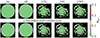 |
Fig. A.1. Rerr statistic for the lines and the adjoining continuum at the photon-packet counts given in Sect. 4. The galaxy shown is AU-1. |
Appendix B: FIR fine-structure lines’ excitation conditions
Table B.1 gives the line excitation conditions for the three fine-structure lines used in this work, the second column gives the energy required to ionize the neutral species to the ionization state in question, followed by the energy difference between the levels resulting in the line. The next two columns give the critical Hydrogen density for the lines originating predominantly in neutral regions, and the electron density for those originating in the ionized regions, respectively. Both values are given for [C II] 158 μm, which originates in both regimes. The last column gives the likely sources of origin of the given line. Table adapted from De Looze et al. (2014b).
Line excitation conditions for the three fine-structure lines used in this work.
Appendix C: Acronyms
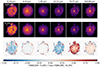 |
Fig. C.1. Comparison of spatial maps generated by SKIRT for TODDLERS (top row), HiiM3 (middle row) models of AU-21, and the normalized difference between the two (bottom row). Columns show different bands centered at wavelengths listed on top. Images use a cube root scale. For each band, the images for both models share the same colormap limits, but the colormap limits may vary between bands. The data has been smoothed using a uniform filter of three pixels. |
Acronyms.
All Tables
Input parameters of the SKIRT radiative transfer model for each of the Auriga components, in addition to the particle and cell positions.
Comparison of kIR values obtained for the Auriga-D sample and the observational sample considered in this work.
Fitting function coefficients and dispersion for the global observational data used in this work.
Fitting function coefficients and dispersion for the resolved observational data used in this work.
Line excitation conditions for the three fine-structure lines used in this work.
All Figures
|
Fig. 1. Example of the fractional SFR contribution originating from recollapsing shells using the method discussed in Sect. 3.3. The system is assumed to have a uniform SFH and has TODDLERS parameters fixed at Z = 0.02, ϵSF = 0.025, ncl = 320 cm−3. The mean value of recollapsing shells is 19%. |
| In the text | |
|
Fig. 2. Comparison of broad-band luminosity scaling relations between the DustPedia sub-sample DPD44 (blue stars) and SKIRT post-processed Auriga galaxies using the two available star-forming regions’ libraries in SKIRT, TODDLERS (red crosses), and HiiM3 (green crosses) at the calibrated parameter values. The Auriga sample in both cases consists of 60 points, including an edge-on and face-on configuration for each of the 30 Auriga galaxies. The rolling median lines use four bins of equal width in the K-band luminosity, LK. |
| In the text | |
|
Fig. 3. Observables generated for the line-emission-based analysis carried out in this work. Left: Spectrum at a resolution R = 3000 in the optical 0.4 − 0.7 μm, right: Selected windows for lines in the FIR, again at R = 3000. At each of these wavelengths, we also generate images at a spatial resolution of 0.5 kpc. |
| In the text | |
|
Fig. 4. Comparison of the median UV-mm SEDs from the SKIRT post-processed Auriga galaxies using the two available star-forming regions libraries in SKIRT, TODDLERS (red) and HiiM3 (green) at the calibrated parameter values. The median is calculated by considering only the exactly edge-on and face-on inclinations. The corresponding filled areas give the range of values encountered for the entire Auriga sample. The lower panels show the ratio of the median SED obtained using TODDLERS and HiiM3 libraries, with the range shown by the filled area only for the fiducial run. |
| In the text | |
|
Fig. 5. Spatially varying IR correction factor, kIR for three Auriga galaxies in a face-on configuration. From left to right: k24, k70, and kTIR for AU-21 (top), AU-23 (middle), and AU-27 (bottom). Each panel also lists the luminosity weighted mean of the value obtained using all the pixels. |
| In the text | |
|
Fig. 6. Mean light-weighted IR correction factors, ⟨kIR⟩IR as a function of the aperture and the inclination using the galaxies in the Auriga-D sample. The aperture is given as a fraction of the optical radius, with the gray region denoting a median aperture of 15−20 kpc of the simulated galaxies. The values from B16 are shown as gray lines. |
| In the text | |
|
Fig. 7. Spatially varying IR correction factor, kIR, shown as a function of the projected sSFR for the Auriga-D sub-sample using the three face-on inclinations. The circular points represent the light-weighted values for individual galaxies at the three inclinations considered in this work. |
| In the text | |
|
Fig. 8. kIR as a function of time for an individual model from the TODDLERS library. |
| In the text | |
|
Fig. 9. SFRD maps (left) and associated MIR-FIR color-color relations (right) for three Auriga galaxies AU-1, AU-2, and AU-21 post-processed with TODDLERS models. The figures in the right column also indicate the PCC value, the SFR of the galaxy inferred using the calibration given in L11 (black value; see Sect. 5.2.1), and the true SFR of the galaxies averaged over 100 Myr (red value). The gray filled contours represent the colors of the KINGFISH sample as reported by G22 while the dashed curve is the relation for NGC-4449 given in C22. |
| In the text | |
|
Fig. 10. Dispersion in Auriga galaxies’ MIR-FIR color-color plot as a function of the non-parametric indicators of galaxy morphology applied to the SFRD maps. The data includes all the three inclinations and all Auriga galaxies except AU-11, which is undergoing a merger. The data-points are color-coded using the Pearson correlation coefficient obtained for the color-color relation for individual galaxies. |
| In the text | |
|
Fig. 11. MIR-FIR color-color diagram considering all the pixels of the Auriga-D galaxies at inclinations 0°, 30°, and 60° along with consolidated “Regime-1” and “Regime-2” data from G22 (gray region). The orange contours represent the data when TODDLERS library is employed, while the green contours are obtained in the case of HiiM3. The darkness of the contour colors represents the density of the pixels on a linear scale. Also shown are the median values for each of the three datasets using round markers of corresponding colors. The dashed black curve is the relation obtained in C18. |
| In the text | |
|
Fig. 12. Fraction of LyC photons that do not participate in the production of Hα at Z = 0.008, 0.02, 0.04 (top) for a population of H II regions generated (as per Sect. 3.3) for the parameters of the TODDLERS models, ϵSF and ncl. The solid line represents the sum of the escape fraction (dashed) and absorption by dust (dotted). Conversion of Hα luminosity to SFR (bottom), using a fixed conversion factor, CHα = 5.5 × 1042, using the same SF region populations and TODDLERS model parameters as the top row. |
| In the text | |
|
Fig. 13. Ratio of the inferred SFR, using a conversion factor of CHα = 5.5 × 1042, applied to the transparent Hα luminosity, compared to the SFR reported by the simulation across the entire Auriga galaxy sample. The color-coding indicates the SFR-weighted metallicity of each Auriga galaxy. |
| In the text | |
|
Fig. 14. Hα maps and attenuation law for one of the Auriga galaxies, AU-1. Panel 1: Transparent Hα surface density, Panel 2: Observed Hα surface density, Panel 3: The observed Balmer decrement, and Panel 4: The attenuation law found by inverting Eq. (7), also shown is the fit to the attenuation law for a simulated Milky-Way galaxy done in T22 (orange) and the fit to the resolved face-on data obtained in this work. |
| In the text | |
|
Fig. 15. Attenuation law obtained by using the Face-on (0° inclination) resolved data for the entire Auriga sample. The circular markers represent the integrated values for Auriga galaxies. The red curve indicates the fit to the data described in Sect. 6.1.2 while the orange curve is the fit from T22. Also shown are the Milky-Way attenuation (purple dashed line) and the input dust model value employed in TODDLERS models (maroon dashed line). |
| In the text | |
|
Fig. 16. Balmer-decrement based attenuation correction for our models when applied to Auriga galaxies as described in Sect. 6.1.2. The ratio of corrected Hα to transparent Hα is shown as a function of the observed Hα luminosity. The circular markers represent the global values while the hexbins represent the kpc-scale data. |
| In the text | |
|
Fig. 17. Line luminosity vs. SFR relation for the Auriga galaxies post-processed with the TODDLERS library. The SFR for the Auriga galaxies is the simulation reported value averaged over 30 Myr. The orange points represent values using an aperture (see Sect. 5.2.1) fR, opt = 1, while the green ones are for fR, opt = 0.33. The straight lines represent various observational relations and the associated filled areas represent the 1σ dispersion on the calibration. |
| In the text | |
|
Fig. 18. Linear fits in the log-log space obtained using the line-emission for Auriga galaxies based on Eq. (10). The shaded area signifies the 1σ dispersion of the fits. The orange fits uses all the pixels, while the green ones only use the brightest 10% of pixels out of the entire Auriga sample for each line. The observational fits for metal-poor dwarf galaxies reported in DL14 are shown in red while those for the [C II] line reported in HC15 are shown in blue. The filled areas represent the 1σ dispersion on the various fits. |
| In the text | |
|
Fig. A.1. Rerr statistic for the lines and the adjoining continuum at the photon-packet counts given in Sect. 4. The galaxy shown is AU-1. |
| In the text | |
|
Fig. C.1. Comparison of spatial maps generated by SKIRT for TODDLERS (top row), HiiM3 (middle row) models of AU-21, and the normalized difference between the two (bottom row). Columns show different bands centered at wavelengths listed on top. Images use a cube root scale. For each band, the images for both models share the same colormap limits, but the colormap limits may vary between bands. The data has been smoothed using a uniform filter of three pixels. |
| In the text | |
Current usage metrics show cumulative count of Article Views (full-text article views including HTML views, PDF and ePub downloads, according to the available data) and Abstracts Views on Vision4Press platform.
Data correspond to usage on the plateform after 2015. The current usage metrics is available 48-96 hours after online publication and is updated daily on week days.
Initial download of the metrics may take a while.