| Issue |
A&A
Volume 692, December 2024
|
|
|---|---|---|
| Article Number | A93 | |
| Number of page(s) | 13 | |
| Section | Planets, planetary systems, and small bodies | |
| DOI | https://doi.org/10.1051/0004-6361/202450659 | |
| Published online | 04 December 2024 | |
The emergence of the MD − Ṁ* correlation in the magnetohydrodynamic wind scenario
1
Dipartimento di Fisica ‘Aldo Pontremoli’, Università degli Studi di Milano,
via G. Celoria 16,
20133
Milano,
Italy
2
European Southern Observatory,
Karl-Schwarzschild-Strasse 2,
85748
Garching bei München,
Germany
3
Leiden Observatory, Leiden University,
PO Box 9513,
2300 RA
Leiden,
The Netherlands
4
Université Paris-Saclay, CNRS, Institut d’Astrophysique Spatiale,
91405
Orsay,
France
5
Dipartimento di Fisica e Astronomia, Università di Bologna,
Via Gobetti 93/2,
40122
Bologna,
Italy
6
Fakultat für Physik, Ludwig-Maximilians-Universität München,
Scheinersts. 1,
81679
München,
Germany
★ Corresponding author; luigi.zallio@unimi.it
Received:
8
May
2024
Accepted:
30
October
2024
Context. There is still much uncertainty around the mechanism that rules the accretion of proto-planetary disks. In recent years, magnetohydrondynamic (MHD) wind-driven accretion has been proposed as a valid alternative to the more conventional viscous accretion. In particular, winds have been shown to reproduce the observed correlation between the mass of the disk MD and the mass accretion rate onto the central star Ṁ*, but this has been done only for specific conditions. It is not clear whether this implies fine tuning or if it is a general result.
Aims. We investigated under which conditions the observed correlation between the mass of the disk MD and the mass accretion rate onto the central star Ṁ*, can be obtained.
Methods. We present mainly analytical calculations, supported by Monte Carlo simulations. We also perform a comparison with the observed data to test our predictions.
Results. In the absence of a correlation between the initial mass M0 and the initial accretion timescale tacc,0 , we find that the slope of the MD − Ṁ* correlation depends on the value of the spread of the initial conditions of masses and lifetimes of disks. Then we clarify the conditions under which a disk population can be fitted with a single power law. Moreover, we derive an analytical expression for the spread of log(MD/Ṁ*) valid when the spread of tacc is taken to be constant. In the presence of a correlation between M0 and tacc,0, we derive an analytical expression for the slope of the MD−Ṁ* correlation in the initial conditions of disks and at late times. In this new scenario, we clarify under which conditions the disk population can be fitted by a single power law, and we provide empirical constraints on the parameters ruling the evolution of disks in our models.
Conclusions. We conclude that MHD winds can predict the observed values of the slope and the spread of the MD−Ṁ* correlation under a broad range of initial conditions. This is a fundamental expansion of previous works on the MHD paradigm, exploring the establishment of this fundamental correlation beyond specific initial conditions.
Key words: protoplanetary disks
© The Authors 2024
 Open Access article, published by EDP Sciences, under the terms of the Creative Commons Attribution License (https://creativecommons.org/licenses/by/4.0), which permits unrestricted use, distribution, and reproduction in any medium, provided the original work is properly cited.
This article is published in open access under the Subscribe to Open model. Subscribe to A&A to support open access publication.
1 Introduction
Proto-planetary disks are the birth environments of planets. In recent decades, significant progress has been made in the field of submillimeter radio astronomy, in particular thanks to the development of the Atacama Large Millimeter/Sub-millimeter Array (ALMA) observatory. Thanks to a transformational improvement in the capabilities of the new generation of telescopes, we now know that disks are substructured, showing gaps, spirals, kinks, and many more features (e.g., Andrews 2020).
In addition to high resolution observations, the study of disk demographics has also advanced significantly. In recent years, it has become possible to collect global disk properties such as submillimeter fluxes (e.g., Mann et al. 2014; Ansdell et al. 2016, 2017; Barenfeld et al. 2016; Pascucci et al. 2016; Cox et al. 2017; Eisner et al. 2018; Cazzoletti et al. 2019; Cieza et al. 2019; Ansdell 2020), disk radii (e.g., Barenfeld et al. 2017; Ansdell et al. 2018; Sanchis et al. 2021), and rates of mass accretion onto the central stars (e.g., Manara et al. 2015; Manara et al. 2017; Alcalá et al. 2017; Manara et al. 2020). This astonishing amount of new data allowed us to start investigating the statistical distributions of disk properties, which make it possible to constrain evolutionary models (e.g., Manara et al. 2023 for a review). However, despite all the progress that has been made, we are still far from a paradigm that can completely describe the formation and evolution of disks (e.g., Morbidelli & Raymond 2016).
Understanding how protoplanetary disks accrete material onto the central star and evolve is of cardinal importance for developing a standard model of planet formation and evolution. Two main physical scenarios have been proposed to explain accretion onto the central star: viscous accretion (e.g., Shakura & Sunyaev 1973; Lynden-Bell & Pringle 1974), which redistributes the angular momentum within the disk (e.g., Pringle 1981; Frank et al. 2002), and magnetohydrodynamic (MHD) wind-driven accretion, where a vertical magnetic field launches a wind that extracts angular momentum from the disk (e.g., Blandford & Payne 1982; Ferreira 1997; Lesur 2021). Despite all the work put in developing these paradigms, there is still significant uncertainty regarding which scenario best describes the evolution of proto-planetary disks, as their key predictions (e.g., the different time evolution of disk radii) are difficult to observe on a statistically significant sample of observations.
In this context, observations have allowed us to find a correlation between the mass of the proto-planetary disk and the mass accretion rate onto the central star (e.g., Manara et al. 2016; hereafter called the MD − Ṁ* correlation). In the viscous paradigm, the MD − Ṁ* correlation naturally arises with a slope close to unity, in agreement with observations (e.g., Lodato et al. 2017; Rosotti et al. 2017); on the other hand, it is still not clear which conditions can produce it in the MHD scenario. In particular, it is uncertain whether it would be a general feature of wind-driven populations or if specific initial conditions would be needed.
Recently, 1D disk evolution models have been proposed to describe the effect of MHD disk-winds on the long-term evolution of disks (Suzuki et al. 2016; Bai 2016; Tabone et al. 2022a). In particular, Tabone et al. (2022a) developed analytical solutions of global disk quantities (i.e., the surface density, the characteristic disk radius, the mass of the disk, and the mass accretion rate) for the MHD wind-driven scenario, and offered some insights about retrieving the correlation. In Tabone et al. (2022b), they show that for a particular set of initial parameters, the MHD model can reproduce the observed correlation in the Lupus region, the spread around this trend, and the decline of the disk fraction. In particular, they qualitatively show that a linear relationship can be obtained assuming no correlation between disk mass and accretion timescale tacc,0. Starting from the solutions of Tabone et al. (2022a), in this work we conduct an extensive analysis to discuss the universality of this result and whether it implies fine tuning.
The scope of the present work is to go beyond the work of Tabone et al. (2022a) to quantify under which initial conditions it is possible to reproduce the observed MD–Ṁ* correlation. In Sect. 2, we show the condition under which it is possible to observe the MD−Ṁ* correlation under the assumption that the initial accretion timescale tacc,0 1 is not correlated with M0. We then analytically derive the slope of the MD−Ṁ*, correlation and its spread as a function of the spread of the disk age t and tacc,0. In Sect. 3, we relax the assumption of no correlation between M0 and tacc,0: we introduce a correlation in the form  , and we analytically derive the slope of the MD−Ṁ* correlation in the initial lifetime conditions of the disks and at late times. Then, by adding a spread in M0 , we show that we can retrieve the observed value of the slope under a broad range of conditions. In Sect. 4, we show that the spread derived in Sect. 2 agrees with the observed spread of log(MD /Ṁ*,). Finally, we present and investigate the
  degeneracy. In Sect. 5, we summarize our conclusions.
2 The MD-Ṁ*, correlation in the absence of a M0 − tacc,0 correlation
Tabone et al. (2022a) find that a proto-planetary disk evolving under the effect of MHD wind torque is governed by the master equation
 (1)
(1)
where αSS is the Shakura-Sunyaev α -parameter, while αDW is its analog for a MHD wind, and λ is the magnetic lever arm. In particular, αDW describes the amount of angular momentum extracted by the wind, while λ determines the mass-loss rate of the wind.
When the viscous torque is neglected (i.e., when MHD winds alone describe the disk evolution and dispersal), assuming αDW and λ to be constant across the disk, and λ to be constant in time, it is possible to solve analytically the master equation, obtaining the surface density profile
 (2)
(2)
where ξ = 1/[2(λ − 1)], and rc is the disk characteristic radius. Tabone et al. (2022a) present solutions where αDW increases as the disk mass decreases, namely as
 (3)
(3)
so that αDW accelerates the evolution of the disk. Here ω is a phenomenological parameter between 0 and 1 that describes the unknown dissipation of the magnetic field. In particular, ω describes the tendency of the magnetization to increase as the disk mass decreases. For example, the case ω = 1 mimics a disk where the magnetic field strength is constant over time, while the case ω = 0 represents a disk with constant magnetization, so that it is dispersed on the same timescale as the mass dissipation. In this set of solutions the disk mass evolves as
 (4)
(4)
and the mass accretion rate Ṁ*, evolves as
 (5)
(5)
where fM,0 is the initial mass ejection-to-accretion ratio
 (6)
(6)
In the end, MD (t) and Ṁ*(t) are controlled by the four independent parameters M0 , fM,0, tacc,0 and ω. In this work, if not otherwise specified we set fM,0 = 2.2 and ω = 0.8.
In this paper, we test the emergence of the MD−Ṁ* correlation. In principle, the accretion onto the central star Ṁ* happens in the innermost region of the disk, where this latter is expected to be turbulent (e.g., Najita et al. 1996, 2009; Carr et al. 2004; Hartmann et al. 2004; Ilee et al. 2014), while in the outer region we assume that the disk is non-turbulent. However, from the modeling point of view, a small turbulent inner disk will always simply re-adjust to the mass accretion rate to which it is fed by the outer wind-driven disk, since locally the viscous timescale is smaller than the disk age. In particular, the accretion rate onto the central star will always quickly adjust to the accretion rate at the inner edge of the non-turbulent region. Hence, we do not explicitly model an inner turbulent region.
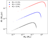 |
Fig. 1 Isochrones of a population of disks with t = 5 Myr for three values of M0 in the MD − Ṁ* plane. The colored dots are Monte Carlo simulations of 105 proto-planetary disks evolving following Eqs. (4), (5) with ω = 0.8, where tacc,0 follows a lognormal distribution centered on the natural logarithm of 1 Myr with a spread of 0.26 dex, while M0 = 0.1, 1.0, 10 M⊙. |
2.1 The emergence of the MD − Ṁ* correlation
When studying populations of disks of similar age, it is of great interest to consider the concept of isochrones (introduced for the first time in Lodato et al. 2017), defined as the location in the MD − Ṁ* plane of the sample of disks that have the same initial mass M0 , same age t, and different accretion timescales tacc,0 .
In Fig. 1, we show the shape of the isochrones of a population of disks. Every dot is a proto-planetary disk, for which the value of MD and Ṁ* are evaluated using Eqs. (4), (5): tacc,0 follows a lognormal distribution centered2 on the natural logarithm of 1 Myr with a spread of 0.26 dex, while M0 = 0.1, 1.0, 10 M⊙. We recover the analytical shape of the isochrone provided in Tabone et al. (2022a). As shown, these curves cannot intrinsically represent a disk population that follows the observed MD − Ṁ* correlation: the boomerang-shaped isochrones cannot be represented by a power law in the form  . These peculiar curves show that disks with high mass and low accretion rates are the ones with the longest tacc,0 , while disks with the lowest mass and low accretion rates are the ones with shortest tacc,0.
To visualize the MD − Ṁ* correlation we set M0 to follow a lognormal distribution rather than taking it as constant. We show in Fig. 2, the results for different values of its spread. We find that the boomerang shape of isochrones, as defined above, is visible in the MD − Ṁ* plane only if the spread of the initial accretion timescale is large enough. Roughly, we can say it tends to be visible for  , where tacc,0 is the initial accretion timescale of the disk, while in the opposite case the points follow a power law behavior.
We note that the observed MD − Ṁ* correlation (Manara et al. 2016) is a power law whose slope is close to unity. In order to sis- tematically determine the values of  and
and  that lead to a correlation between MD and Ṁ*, we use the coefficient of determination R2. Combining a visual inspection of the MD − Ṁ* plane with the evaluation of R2 from the best power law fit for each disk population, we derived a conservative “rule of thumb”: R2 ≳ 0.5. If R2 ≳ 0.5, the disk population can be safely fitted in the MD − Ṁ* with a single power law. We note that this general rule is only informative of the goodness of fit for a disk population in the MD − Ṁ* plane with a single power law, and that we investigate under which conditions we can derive a linear correlation between MD and Ṁ* (see below). We also note that our criterion is in agreement with the correlation coefficient found in Manara et al. (2016) of r = (0.56 ± 0.12), which changes to r = (0.7 ± 0.1) when the upper limits are considered in the analysis.
In Fig. 3 we show the value of R2 (the coefficient of determination) measured on a large grid of models. In these plots we set M0 and tacc,0 to follow a lognormal distribution centered on the natural logarithm of 0.1 M⊙ and 1 Myr, respectively, and we chose ω = 0.8. The hatched contours represent the regions where R2 = 0, and the dashed line represents the points where  . Figure 3 shows the regions of the
  plane that allow alow or high value of R2. Starting from these plots, we can extract different combinations of values for
  and
and  , and we can visualize which of them, at different ages and for different values of ω, yield a power law correlation in the MD − Ṁ* plane. We chose to span from very young (t = 105 yr) to evolved disk populations (t = 2.5 × 10⁶ yr) to fully explore the parameter space.
Tabone et al. (2022b) show that there is no requirement to fine-tune ω to reproduce the observed accretion rates and disk masses, although explaining the rapidity of disk dispersal disfavors values of ω ~ 0; in particular, if 0.5 ≲ ω < 1 these latter experience a steeper drop before being dispersed and in this way reproduce the observed distribution. Hence, we chose ω = 0.8, which is bracketed by the ω = 0.5 and ω = 1 solutions shown by Tabone et al. (2022b). For completeness, in Appendix A, we show the same plots as in Fig. 3, but for the extreme cases of ω = 0.2 and ω = 1, highlighting how the results of this work also hold for different values of ω.
From Fig. 3, we note that our criterion R2 ≳ 0.5 is very roughly described by
 (7)
(7)
In general, if Eq. (7) is satisfied, the population of disks that we consider can be described, in first approximation, as having constant tacc,0. For such a population, the slope of the MD − Ṁ* correlation is γ = 1 (for the analytical calculations, see Appendix B).
In Fig. 4, we show the MD − Ṁ* correlation in the regime described by Eq. (7). Here, M0 and tacc,0 follow a lognormal distribution centered on the natural logarithm of 0.1 M⊙ with a spread of 1.5 dex and on the natural logarithm of 2 Myr with a spread of 0.15 dex, respectively. The gray line is the fit of a single power law, which results in γ = 1. It is important to note that 4 shows that if  , we would not be observing a linear correlation between MD and Ṁ* ; we would instead see the boomerang isochrone shape shown in Fig. 1, which likewise depends on the value of ω.
We note that Eq. (7) is only an approximate criterion. The exact criterion under which the MD − Ṁ* correlation is a power law with a slope of unity is more complex and depends on the age and on the value of ω. In particular, we find that for low values of ω (see Appendix A) the correlation is harder to get, in particular at late time. For detailed studies we thus recommend using Figs. 3, A.1, and A.2 to identify the regions of the parameter space that give a correlation instead of Eq. (7).
We can summarize the results obtained as follows:
In the case in which there is no spread in M0 , a boomerangshaped isochrone appears in the MD − Ṁ* plane;
In the limit
 , the slope of the MD − Ṁ* relation is exactly 1, a result that can also be obtained analytically;
In the general case, we find that the correlation is recovered when the spread in initial disk mass is typically larger than the spread in initial accretion timescale. This rule of thumb can be refined using Figs. 3, A.1, and A.2.
However, observations provide us with more than a correlation; they give the spread around this correlation and the power law index. In particular, observational results (e.g., Manara et al. 2016; Testi et al. 2022) consistently find values of the MD − Ṁ* correlation that are <1 along with a large spread. Therefore, in the next section, we study under which conditions we can retrieve the observed value of the slope of the MD − Ṁ* correlation and its spread.
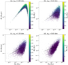 |
Fig. 2 MD − Ṁ* plane for different values of |


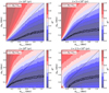 |
Fig. 3
|


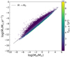 |
Fig. 4 MD − Ṁ* correlation with ω = 0.8 and t = 2 Myr. The colored dots are Monte Carlo simulations of 105 proto-planetary disks evolving following Eqs. (4), (5) where M0 and tacc,0 follow a lognormal distribution centered, respectively, on 0.1 M⊙ with a spread of 1.5 dex and on 2 Myr with a spread of 0.15 dex. The gray line represents the best fit of a single power law, for which γ = 1. |
2.2 The slope and the spread of the MD − Ṁ* correlation as a function of  and
and 
In order to constrain the values of  and
and  that can repro- duce the observed slope and spread of the MD − Ṁ* correlation, we performed a linear regression of the disks in the MD −Ṁ* plane for different combinations of
  and
and  . In Fig. 5, we show the results of our analysis. Here, the colored stripes in the
  plane represent the regions of the parameter space that predict values of the slope y and of the spread σ of the MD − Ṁ* correlation in agreement with the observed values. In a similar fashion to the analysis performed in Lodato et al. (2017), we show in orange the region γ ∈ [0.5,0.9], while in light blue the region σ ∈ [0.55,0.71] dex. In contrast with Lodato et al. 2017 and Tabone et al. 2022b, we neglected the effect of accretion variability and the uncertainties on the mass estimates. This means that the populations tend to underestimate the spread in MD/Ṁ*. In this plot, t = 2 Myr, ω = 0.8, and M0 and tacc,0 follow a lognormal distribution centered on the natural logarithm of 0.1 M⊙ and 2 Myr, respectively. The cross represents the work of Tabone et al. (2022b). Fig. 5 shows that it is possible to retrieve the observed values of the slope and the spread of the MD− Ṁ* correlation for
 ![${\sigma _{{M_0}}} \in [0.50,1.50]$](/articles/aa/full_html/2024/12/aa50659-24/aa50659-24-eq31.png) and
and ![${\sigma _{{t_{{\rm{acc}}{\rm{.}}0}}}} \in [0.40,0.75]$](/articles/aa/full_html/2024/12/aa50659-24/aa50659-24-eq32.png) .
.
We note that the results obtained here are valid for a fixed age t, a value of ω = 0.8, and the fixed median values M0 = 0.1 M⊙ and tacc,0 = 2 Myr. As we show in Appendix A, changing ω will change the derived values of  and
and  , but it remains true that it is possible to retrieve the observed slope and the spread of the MD− Ṁ* correlation for a wide range of spreads in disk mass and accretion timescales in the initial conditions. We also note that in Fig. 5 not all the populations fit the disk fraction. As discussed below and in Tabone et al. (2022b), a typical value of
  dex needs to be adopted to fit the observed decline of disk fraction with cluster age.
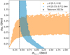 |
Fig. 5
|


2.3 The spread of log(MD− Ṁ*) as a function of the spread in t and tacc
Testi et al. (2022) and Somigliana et al. (2023) show that the spread of the accretion timescale MD/Ṁ* is a fundamental observable for disk population studies. Considering Eqs. (4), (5), we can evaluate the dimensionless spread of the accretion timescale when Ṁ* ∝ MD. Using the propagation of errors (see more details in Appendix C) on log(MD/Ṁ*), the dimensionless spread is
 (8)
(8)
where we use the notation 〈tacc,0〉 and 〈t〉 to remark this is the median value for the population, and we also allow for the possibility of an age spread σt in the population. This result is equivalent to the spread of the MD − Ṁ* correlation for a slope mildly different than 1, but we note that if the MD − Ṁ* correlation differs substantially from linearity, then Eq. (8) is not valid anymore.
The fundamental assumption underlying Eq. (8) is that  is taken to be constant in time. In reality, this value should be computed only over the population of surviving disks. It is not necessarily true that it stays constant as, while evolving with time, a disk population loses the fastest evolving disks; as a consequence,
  should decrease as time passes. However, as noted in the work of Somigliana et al. (2023), the spread on the accretion timescale decreases slowly in time in the MHD wind-driven scenario (a factor of 0.1 dex within 2 Myr). Therefore, Eq. (8) can be considered valid for young star-forming regions. Moreover, we note that the spread of log(MD /Ṁ*) is equal to that of the MD − Ṁ* correlation when the slope of the correlation is exactly 1. Therefore, in first approximation, the expression reported in Eq. (8) gives us an estimate of the order of magnitude of the spread of the MD − Ṁ* correlation, as further discussed in Sect. 4.1.
In Fig. 6, we show the spread of log(MD /Ṁ*) when t follows a lognormal distribution centered on the natural logarithm of 1 Myr, and σt = 0.43 dex. The black line is computed as the standard deviation from the Monte Carlo simulations of 105 disks that follow a lognormal distribution in t, tacc and M0. In particular, the value of σ(log(MD /Ṁ*)) is evaluated for 102 values of  that span [0, 1.1] dex, while σt = 0 dex. Here, M0 and tacc follow a lognormal distribution centered, namely, on the natural logarithm of 5 Myr for tacc and on the natural logarithm of 0.1 M⊙ for M0. The spread of log(MD/Ṁ*) is independent of the spread in M0 under the conditions for which Eq. (8) holds, which is that the slope of the MD − Ṁ* correlation is close to unity. In Fig. 5 we see, as we get close to γ = 1, that the cyan band representing the spread of the MD − Ṁ* correlation becomes vertical, while as we move away from those values the dependence on
  appears.
As shown in Testi et al. (2022) and Somigliana et al. (2023), the spread on the accretion timescale is an important observable that can be easily obtained from the data. We show a comparison with observations in Sect. 4.1.
Until now in the current paper, we considered disk populations for which M0 and tacc,0 are not correlated. First, we derived a general criterion for which we can retrieve a population of disks in the MD − Ṁ* plane that can be fitted with a single power law. Second, we studied under which initial conditions it is possible to reproduce the observed slope and spread of the MD − Ṁ* correlation. Finally, we provided an approximated analytical expression for the spread on the accretion timescale log(MD /Ṁ*). In the following, we study the emergence of the MD − Ṁ* correlation when M0 is correlated to tacc,0.
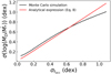 |
Fig. 6 Spread of the MD − Ṁ* correlation as a function of |

3 The MD − Ṁ* correlation in the presence of a M0−tacc,0 correlation
So far we have considered the initial accretion timescale tacc,0 to be uncorrelated with the initial mass of the disk M0. However, this is not necessarily the case. In the following, we assume a correlation between M0 and tacc,0 in the form
 (9)
(9)
Inserting Eq. (9) in Eqs. (4), (5), it is not possible to find an analytical derivation of the slope in the form of Eq. (B.3). However, it is possible to study the analytical behavior of the slope in the initial and final stages of the evolution of the disk, starting from the definition (following Tabone et al. 2022a) of
 (10)
(10)
as the disk dispersal time.
3.1 The MD − Ṁ* correlation at initial time
When taking a population of disks without spread in M0 , in the initial conditions (i.e., t/tdisp ≪1) we find that the slope is γ = 1 −1/ф (see Appendix D.1 for more details).
In Fig. 7, we show the MD − Ṁ* correlation for a disk population (dots) of 105 disks ruled from Eqs. (4), (5), where M0 is given by Eq. (9). Here, ф = 0.8, ω = 0.8, t = 0 yr, and tacc,0 follows a lognormal distribution centered on the natural logarithm of2 Myr with a spread of 0.13 dex. The black line shows the analytical MD − Ṁ* correlation (Eq. (D.2)), which agrees remarkably well with the Monte Carlo simulations.
3.2 The slope close to disk dispersal
When considering a population of disks without spread in M0 , close to dispersal (i.e., t/tdisp ~ 1) we find that γ = 1 − ω (see Appendix D.2 for more details). This is an unexpected result, as the slope appears to reach a specific value that is independent from the initial correlation between M0 and tacc,0. This occurs when a disk population is close to dispersal because all the disks also share a similar tacc,0 and, as a consequence, a similar M0 (as they are linked to each other). Thus, when t/tdisp ~ 1, the correlation between M0 and tacc,0 is lost and the memory of the initial conditions is forgotten. Tabone et al. (2022a) find a similar result, even without explicitly introducing a correlation. This supports the previous statement that, taking a population of disks that is about to be dispersed, it is only possible to observe the final evolutionary track of the disk (for which  ), thus losing any possibility of detecting the initial correlation between M0 and tacc,0.
In Fig. 8, we show the MD−Ṁ* correlation for ϕ = 0.8, ω = 0.8, and t = 3 Myr, where the other parameters are the same as in Fig. 7. We see in this case that the MD−Ṁ* correlation has a bent shape that could be better described by a double power law. We are interested in the left part of the plot, where MD ≲ 10−2 M⊙ (i.e., when the disk lifetime is similar to the disk dispersal time). The black line shows Eq. (D.6): the slope of the theoretical line (black) coincides with the MD−Ṁ* correlation in the above-cited region of the MD−Ṁ* plane, showing that when t ~ tdis p, the slope approaches the value γ = 1 − ω. The right part of Fig. 8 instead shows the disks that are still evolving, and hence still near the condition t/tdisp ≪ 1; we see that the slope here inverts its trend, in agreement with the value 1 − 1 /ϕ that we derived in Sect. 3.1.
In Appendix E, we show the calculation of the spread of the MD−Ṁ* correlation when  . The (trivial) results are in continuity with what we describe in Sect. 2.3.
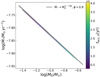 |
Fig. 7 Slope of the MD−Ṁ* correlation with ϕ = 0.8, ω = 0.8, and t = 0 yr. The dots are Monte Carlo simulations of 105 proto-planetary disks ruled from Eqs. (4) and (5) where M0 follows Eq. (9) and tacc,0 follows a lognormal distribution centered on the natural logarithm of 2 Myr with a spread of 0.13 dex. The black line represents Eq. (D.2). |
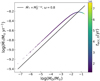 |
Fig. 8 Slope of the MD−Ṁ* correlation with ϕ = 0.8, ω = 0.8, and t = 3 Myr. The colored dots are Monte Carlo simulations of 105 protoplanetary disks ruled from Eqs. (4) and (5), where M0 follows Eq. (9) and tacc,0 follows a lognormal distribution centered on the natural logarithm of 2 Myr with a spread of 0.13 dex. The black line represents Eq. (D.6). |
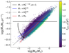 |
Fig. 9 MD−Ṁ* correlation with ϕ = 1, ω = 0.8, and t = 3.5 Myr. The dots are Monte Carlo simulations of 105 proto-planetary disks evolving following Eqs. (4) and (5), where M0 follows Eq. (9) and tacc,0 follows a lognormal distribution centered on the natural logarithm of 5 Myr with a spread of 0.13 dex. In addition, M0 is then generated following a lognormal distribution with the values of tacc,0 following Eq. (9) with a spread of 0.43 dex. The black line represents Eq. (D.2), the gray line is the best-fitting power law for the population, resulting in |


3.3 The role of  in the MD−Ṁ* correlation
If tacc,0 is generated following a lognormal distribution with a spread and  is satisfied, it is reasonable to think that M0 should also have a spread of its own (i.e., the spread in M0 reflects the fact that different stars living in the same stellar population have different masses, not only different initial timescales). To ensure that our populations have a spread in M0, we initially evaluated M0 with Eq. (9); then M0 was extracted with a lognormal distribution, with fixed spread, centered on the previously determined values of M0. In Fig. 9, once the spread in M0 is added, we see the appearance of the linear MD−Ṁ* relation. Here we show a population of disks identical to the one in Fig. 8, but we add a spread in M0 of 0.43 dex. The addition of
  hides the track shown in Fig. 8. Moreover, the slope becomes steeper as
  increases, going toward the linear behavior, which is plotted in red. As a reference, we plotted in gray the best-fitting power law for the population, resulting in a slope of 0.83; in blue the best-fitting power law for a population with
  dex, resulting in a slope of 0.65; while in black we report the slope obtained in Eq. (D.3).
We draw two main conclusions from this. First, it is still possible to derive the slope of the MD−Ṁ* correlation with a value different than unity after the introduction of the correlation  . It is also possible to tune the value of the MD−Ṁ* slope, changing the values of ϕ and
  : we discuss this in Sect. 4.2. Second, the addition of
  deletes the canonical signature of the slope shown in Figs. 7 and 8. This leads to a dramatic observational conclusion: it is not possible to directly observe the expected analytical signature of the slope because of the natural existence of spread in M0.
3.4 Describing the MD−Ṁ* correlation by a single power law
It is relevant to emphasize that, after the introduction of a spread in M0, the bent shape of the MD−Ṁ* correlation shown in Fig. 8 can still be recovered, but only for very low values of  .3 Figure 8 clearly shows that a single power law cannot properly fit the evolutionary track of the disks: a double power law seems much more appropriate. Hence, we conducted a test in order to quantitatively understand when a single power law starts to fit a disk population.
First, we introduced a broken double power law in the form
 (11)
(11)
where  is not a free parameter as the piecewise function is defined to be continuous in MD = x0. Then, after setting t = 3 Myr, we fitted both Eq. (11) and the equation of a single power law in the form
 (12)
(12)
to the Ṁ*−MD plane for different values of  , namely
 ![${\sigma _{{M_0}}} \in \left[ {0,0.022} \right]$](/articles/aa/full_html/2024/12/aa50659-24/aa50659-24-eq66.png) dex. The other parameters for the disk population are the same as in Fig. 9. Since Eq. (11) is defined based on six free-parameters (x0, k1, a, b, c, d), while Eq. (12) on only two (a, ζ), we performed the fit using the Bayesian Information Criterion (BIC), with the Python package RegscorePy.bic.
dex. The other parameters for the disk population are the same as in Fig. 9. Since Eq. (11) is defined based on six free-parameters (x0, k1, a, b, c, d), while Eq. (12) on only two (a, ζ), we performed the fit using the Bayesian Information Criterion (BIC), with the Python package RegscorePy.bic.
In Fig. 10, we show that the BIC is minimized from the double power law in the regime ![${\sigma _{{M_0}}} \in \left[ {0,0.01} \right]$](/articles/aa/full_html/2024/12/aa50659-24/aa50659-24-eq67.png) dex, hence showing that for very low values of
dex, hence showing that for very low values of  , the MD−Ṁ* correlation is better fitted with a double power law. However, as little spread in M0 is added, the red and the black curve become indistinguishable, highlighting the fact that those disk populations can be fitted both with a single or a double power law4.
From this we can conclude that when a little spread in Mo is added, the MD−Ṁ* correlation can be described by a single instead of a double power law. Thus, it is reasonable to use a single power law to fit the MD−Ṁ* correlation. We show the same plot of Fig. 10 in Appendix F for ![${\sigma _{{M_0}}} \in \left[ {0,0.43} \right]$](/articles/aa/full_html/2024/12/aa50659-24/aa50659-24-eq69.png) dex.
dex.
4 Comparison with the data. Empirical constraints on the spreads
4.1 MHD wind-driven accretion can reproduce the observed spread of log(MD−Ṁ*)
To assess whether MHD winds can reproduce both disk lifetimes and the observed spread in log(MD−Ṁ*), we conducted the following analysis.
So far, the spread in tacc,0 has been considered as a free parameter. As shown by Tabone et al. (2022b), though with a different ansatz for the distribution of tacc,0, the observed disk fraction sets both  and the median values of tacc,0. Following the work of Tabone et al. (2022b), we fitted the disk fraction (represented as the fraction of sources that show IR excess) reported in Fedele et al. (2010) and references therein. We first defined our disk fraction as the ratio of disks that, at a certain time t, satisfies the condition
 (13)
(13)
Then we performed a fit using the complementary cumulative distribution function (CCDF) assuming a lognormal distribution of tdisp. In this way, we find the parameters that describe the probability for a disk population to satisfy Eq. (13).
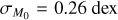
In Fig. 11, we show the results of the fit. We find that tdisp follows a lognormal distribution with a median value  Myr and a spread
  dex. After some sim-pie algebra deriving from Eq. (10), we find that the median value of the accretion timescale is
  Myr and the spread is
  dex. With these values, we evaluated the spread of the accretion timescale using Eq. (8) with t = 1.5 Myr and σt = 05 dex, obtaining σ(log(MD/Ṁ*)) = 1.01 dex.
We compared this value with the spread of the accretion timescale evaluated from the data found in Testi et al. (2022) for the four populations of L1688, Lupus, ChaI, and USco. We removed the upper limits from the sample and considered only the systems for which M* > 0.15 M⊙, in agreement with Testi et al. (2022). For L1688 and Lupus, we obtained values of σ(log(MD/Ṁ*)) that are closely comparable with that reported above, more specifically σ(log(MD/Ṁ*))L1688 = 0.86 dex, σ(log(MD/Ṁ*))Lupus = 1.08 dex. As we moved to the older region of ChaI, we obtained the higher spread σ(log(MD/Ṁ*))ChaI = 1.62 dex, a value that increases even more for USco, the oldest region of the sample, for which we obtained σ(log(MD/Ṁ*)US co = 2.02 dex. The reason behind these higher spreads is that to evaluate σ(log(MD/Ṁ*)), we assumed that the distribution of σ(log(MD/Ṁ*) is normal. This assumption is valid only for young populations of disks (e.g., L1688, Lupus, and at most ChaI); as the population evolves in time, we lose disks, and the distribution of σ(log(MD/Ṁ*) significantly deviates from the starting distribution.
We hence conclude that the spread predicted using Eq. (8) can reproduce well the spread of the accretion timescale for young populations of disks. This result is in agreement with the analysis of Tabone et al. (2022a), but in this work we assumed a lognormal distribution to fit for tdisp, as already performed by Somigliana et al. (2023), and we applied the results to different stellar regions. We furthermore recall that for our calculation we set σt = 0 dex, and we neglected accretion variability and mass uncertainty, so the value of σ(log(MD/Ṁ*)) that we predicted must be considered as a lower limit.
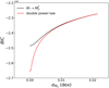 |
Fig. 10 BIC as function of |

![${\sigma _{{M_0}}} \in \left[ {0,0.022} \right]{\rm{dex}}$](/articles/aa/full_html/2024/12/aa50659-24/aa50659-24-eq71.png)

 |
Fig. 11 Disk fraction as a function of the cluster age (data from Fedele et al. 2010 and references therein), with the fit of the CCDF of tdisp. From the fit, we obtain tdisp = 2.37 Myr and |

4.2 Empirical constraints on  and ϕ
and ϕ
We conclude this work by showing the existence of a degeneracy between ϕ and  . As pointed out in Sect. 3.3, the slope of the MD−Ṁ* correlation is affected by both ϕ and
  . From Monte Carlo simulations it is possible to investigate the
  space in order to constrain for which values of ϕ and
  it is possible to retrieve a slope γ ∊ [0.5 ,0.9], with a spread on the MD−Ṁ* correlation σ ∊ [0.55 ,0.71] dex (Manara et al. 2016). To do this, we simply evaluated γ and the spread of the MD−Ṁ* correlation with a linear regression of the disks residing in the MD−Ṁ* plane. Each Monte Carlo simulation consists of 104 disks evolving according to Eqs. (4), (5), where
  .
.
In Fig. 12, we show the  plane with the corresponding values of γ. The coloured regions in the
  plane show the value of the slope and of its spread obtained via linear regression of a whole population of disks generated with specific values of ϕ and
  . In a similar fashion to the analysis performed in Lodato et al. (2017), we show in orange the region γ ∊ [0.5 , 0.9], while in light blue the region σ ∊ [0.55 , 0.71] dex. In this case t = 2 Myr, ω = 0.8, and tacc,0 follows a lognormal distribution centered on the values derived in Sect. 4.1. For comparison, we marked with a cross the region covered in Tabone et al. (2022b).
Following Sect. 3.3, we found that γ tends toward unity as  increases, regardless of the value of ϕ. However, there is a whole region of the
  plane that allows values of γ ≠ 1; this confirms the existence of a degeneracy between ϕ and
  . Moreover, following Fig. 12, we can constrain the ensemble of values of
  that allow us to have the observed values of γ and σ; we see that only values of ϕ ∊ [−2,1] and
 ![${\sigma _{{M_0}}} \in \left[ {0,1.75} \right]$](/articles/aa/full_html/2024/12/aa50659-24/aa50659-24-eq93.png) dex are allowed. Figure 12 leads us to understand that for higher values of ϕ we need higher values of
dex are allowed. Figure 12 leads us to understand that for higher values of ϕ we need higher values of  in order to retrieve the observed MD−Ṁ* correlation. This can be explained as follows: the stronger the correlation between M0 and tacc,0 is, the bigger the spread in M0 must be in order to break the bent shape shown in Fig. 8.
To conclude, we report that the range of values we found for σM0 is in agreement with the results found in Tabone et al. (2022a) for modeling the Lupus population, although there they explored only the case with no correlation between M0 and tacc,0. Moreover, we note that in this section we show a procedure to constrain the parameters that rule the evolution of MHD wind-driven disks in the presence of a correlation between M0 and tacc,0.
From Fig. 12, we understand that we can obtain values of the slope of the MD−Ṁ* correlation which are compatible with Manara et al. (2016), regardless of the initial conditions of the disk populations. We hence conclude that it is possible to derive the slope of the MD−Ṁ* correlation in the MHD wind-driven scenario under a broad range of conditions, a result that shows that the MD−Ṁ* correlation can also be easily obtained for this evolutionary paradigm.
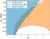 |
Fig. 12
|


5 Conclusions
In this paper, we investigated under which conditions the MD−Ṁ* correlation emerges in the MHD wind-driven evolutionary scenario.
We derived and analyzed the parameters that rule the appearing and tuning of the MD−Ṁ* correlation starting from the analytical solutions given by Tabone et al. (2022b). From our analysis we reach the following conclusions:
- (i)
Introducing a spread
 , we obtain the correlation between the mass of the disk MD and the accretion onto the central star Ṁ*. This holds as long as
  , a conservative criterion that is compatible with the general rule of thumb R2 ≳ 0.5. In the opposite case, the MD−Ṁ* correlation tends to the boomerang-shaped isochrone introduced by Lodato et al. (2017) for the viscous case and studied by Tabone et al. (2022a), and Tabone et al. (2022b) for the wind case, which look significantly different from the observed correlation;
 - (ii)
It is possible to derive a slope and a spread of the MD−Ṁ* correlation comparable to that found in Manara et al. (2016) varying
 and
and  . Hence, it is possible to derive the observed slope and spread of the MD−Ṁ* correlation under a range of initial conditions;
 - (iii)
Neglecting the time evolution of the accretion timescale, we derived an analytical expression for the spread of the accretion timescale log(MD−Ṁ*). The predictions arising from this formula are in agreement with the observed order of magnitude of σ(log(MD−Ṁ*)) evaluated for young populations of disks (Testi et al. 2022);
- (iv)
We introduced a correlation
 to understand if we can still derive the observed slope and spread of the MD−Ṁ* correlation. We analytically derived a slope γ = 1 − 1/ϕ in the initial conditions, and a slope γ = 1 − ω close to dispersal.
Furthermore, we found that the addition of a minimal spread in the initial disk mass distribution
 affects the slope of the MD−Ṁ* correlation. In particular, we showed that we can fit the MD−Ṁ* correlation with a single power law because of the existence of
  ;
; - (v)
We studied the degeneracy between ϕ and
 , and we confirmed that we can obtain values of the slope and of the spread of the MD−Ṁ* correlation in agreement with Manara et al. (2016) for a broad range of values on both
  and ϕ.
This work is the natural follow-up of the work of Tabone et al. (2022a) and Tabone et al. (2022b). We investigated in greater detail the emergence of the MD−Ṁ* correlation and demonstrated that the slope of the correlation is controlled by the correlation among the parameters describing the initial conditions (physically speaking, the star formation process). With this, we reached the fundamental conclusion that MHD wind-driven disks can reproduce the observed slope of the MD−Ṁ* correlation under a broad range of initial conditions. Therefore, no fine tuning of the model parameters is needed in the MHD scenario, but reproducing the correlation does exclude some regions of the parameter space, as shown by Figs. 5, and 12. While in this paper we focused only on the MHD wind scenario, our work implies that the observed MD−Ṁ* correlation cannot be used to discriminate between MHD winds and the viscous model. However, the correlation still constrains the model parameters for each scenario, as shown, for example, by our work and Lodato et al. (2017).
Data availability
All data used in this work are publicly available and can be found at the corresponding cited works. The scripts that have been used for this work will be shared under reasonable request to the corresponding author.
Acknowledgements
We are thankful to the anonymous referee who helped improve the clarity of the paper. The authors acknowledge support from the European Union (ERC Starting Grant DiscEvol, project number 101039651), from Fondazione Cariplo, grant No. 2022-1217, from the European Union’s Horizon 2020 research and innovation programme under the Marie Sklodowska-Curie grant agreement No 823823 (Dustbusters RISE project), and from the ERC Synergy Grant “ECOGAL” (project ID 855130). Views and opinions expressed are, however, those of the authors only and do not necessarily reflect those of the European Union or the European Research Council. Neither the European Union nor the granting authority can be held responsible for them. We thank Carlo Manara for the very useful comments he provided for ensuring the correctness of this work. Moreover, we thank Giacomo Lucertini for the useful discussions in statistics, Edoardo Merli for IT support, Davide Giovagnoli for interesting dialogues in mathematics, Enrico Ragusa and Chiara Scardoni for the many chats in physics.
Appendix A The  plane for different values of ω
In Figs. A.1, A.2 we show the  plane for ω = 0.2 and ω = 1.0, respectively. All the other parameters are the same as the ones presented in Fig. 3. We highlight that the “rule of thumb” derived in Sect. 2 holds also for these “extreme” values of ω. Moreover, we note that, in Fig. A.1 for evolved populations our general criterion R2 ≳ 0.5 does not correspond anymore necessarily to the region
  . The reason for this is shown in Fig. A.3: for evolved populations, when ω → 0, the disks collect around the evolved region of the “boomerang-shaped” isochrone, thus being effectively fitted with a single power law. However, we note that our criterion is very general, therefore any simulated population based on Figs. A.1, A.2, 3, must be checked directly in the MD−M* plane.
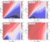 |
Fig. A.1
|


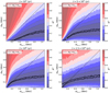 |
Fig. A.2
|


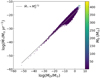 |
Fig. A.3 MD−Ṁ* correlation with ω = 0.2 and t = 2.5 Myr. The colored dots are Monte Carlo simulations of 105 proto-planetary disks evolving following Eqs. (4), (5) where M0 and tacc,0 follow a lognormal distribution centered, respectively, on the natural logarithm of 0.1 M⊙ with a spread of 0.8 dex and on the natural logarithm of 1 Myr with a spread of 0.4 dex. The gray line represents the best fit to the population, resulting in a slope γ = 0.72. |
Appendix B The slope of the MD−Ṁ* correlation when tacc,0 is constant: analytics
Considering tacc,0 as a constant value, Eq. (5) can be seen as
 (B.1)
(B.1)
Taking the hint from the work of Manara et al. 2016, it is possibile to investigate the analytical behavior of disks evolving according to Eq. (B.1), assuming that
 (B.2)
(B.2)
Performing the logarithmic derivative on Eq. (B.2), the slope γ results in the constant
 (B.3)
(B.3)
Appendix C The spread of the MD−Ṁ* correlation as function of the spread in t and tacc: analytics
Starting from Eqs. (4), (5), the ratio MD−Ṁ* reads
 (C.1)
(C.1)
Neglecting the covariance term between t and tacc,0, the spread of log(MD−Ṁ*) correlation is obtained with a simple propagation of errors as
![$\eqalign{ & \sigma \left( {\log \left( {{M_D}/{{\dot M}_*}} \right)} \right) = \left[ {\sigma _{{t_{{\rm{acc }},0}}}^2{{\left( {{{\partial \left( {\log \left( {{M_D}/{{\dot M}_*}} \right)} \right)} \over {\partial \log \left( {{t_{{\rm{acc}},0}}} \right)}}} \right)}^2} + } \right. \cr & \,\,\,\,\,\,\,\,\,\,\,\,\,\,\,\,\,\,\,\,\,\,\,\,\,\,\,\,\,\,\,\,\,\,\,\,\,\,\,\,\,\,\,{\left. {\sigma _t^2{{\left( {{{\partial \left( {\log \left( {{M_D}/{{\dot M}_*}} \right)} \right)} \over {\partial \log (t)}}} \right)}^2}} \right]^{1/2}}, \cr} $](/articles/aa/full_html/2024/12/aa50659-24/aa50659-24-eq118.png) (C.2)
(C.2)
which gives Eq. (8) after some simple algebra. We note that the quantity  is the spread of the accretion timescale. This quantity, due to dispersal of the fastest evolving disks, decreases as a function of time. However, for our calculations, we keep it fixed to its initial value.
Appendix D The slope of the MD−Ṁ* correlation when  : analytics
D.1 The slope for t/tdisp << 1
Injecting Eq. (9) into Eq. (4), we find that, in the initial conditions of the evolution of the disk, namely when t/tdisp << 1,
 (D.1)
(D.1)
Including this result in Eq. (5), after the trivial substitution of Eq. (9) in Eq. (5), we obtain
 (D.2)
(D.2)
The logarithmic derivative gives the slope in the form
 (D.3)
(D.3)
D.2 The slope for t ~ tdisp
We derive the slope in the final life-time conditions of a disk starting by choosing ϵ to be arbitrarily small. Then, inserting
 (D.4)
(D.4)
in Eqs. (4), (5) after the previous substitution of Eq. (9), ϵ is given by
 (D.5)
(D.5)
After some algebra, it is obtained that
 (D.6)
(D.6)
which leads to a slope of the form
 (D.7)
(D.7)
Appendix E The spread of the MD−Ṁ* correlation when 
E.1 The spread when  and t << tdisp
Following Sect. 2.3, the calculations for the spread when  lead to
 (E.1)
(E.1)
This shows the trivial fact that, in the initial conditions, the spread of the correlation depends uniquely on the spread of tacc,0, a result already shown in Fig. 6.
E.2 The spread when  and t ~ tdisp
A similar result is obtained when t ~ tdisp, obtaining
 (E.2)
(E.2)
It is clear that the more t approaches the value of tdisp, the littler is the value of ϵ. In the limit for ϵ → 0, Eq. (E.2) gives σ(log(Md/Ṁ*) → 0: a valid result that reflect the fact that when the disk is about to die, the slope of the Md−Ṁ* correlation inevitably tends toward the value 1 − ω.
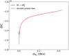 |
Fig. E.1 BIC as function of |

![${\sigma _{{M_0}}} \in [0,0.43]$](/articles/aa/full_html/2024/12/aa50659-24/aa50659-24-eq135.png)

Appendix F The likelihood and the BIC in a wider  range
range
In Fig. E.1 we show the same results of Fig. 10, in a range ![${\sigma _{{M_0}}} \in [0,1]$](/articles/aa/full_html/2024/12/aa50659-24/aa50659-24-eq138.png) . As can be seen, for significant values of
. As can be seen, for significant values of  , the Ṁ* − MD loses the double power law behavior in favor of a single power law written in the form of Eq. (12).
References
- Alcalá, J. M., Manara, C. F., Natta, A., et al. 2017, A&A, 600, A20 [NASA ADS] [CrossRef] [EDP Sciences] [Google Scholar]
- Andrews, S. M. 2020, ARA&A, 58, 483 [Google Scholar]
- Ansdell, M. 2020, in Five Years After HL Tau: A New Era in Planet Formation (HLTAU2020), 29 [Google Scholar]
- Ansdell, M., Williams, J. P., van der Marel, N., et al. 2016, ApJ, 828, 46 [Google Scholar]
- Ansdell, M., Williams, J. P., Manara, C. F., et al. 2017, VizieR Online Data Catalog: ALMA survey of protoplanetary disks in sigma Ori (Ansdell+, 2017), VizieR On-line Data Catalog: J/AJ/153/240 [Google Scholar]
- Ansdell, M., Williams, J. P., Trapman, L., et al. 2018, ApJ, 859, 21 [NASA ADS] [CrossRef] [Google Scholar]
- Bai, X.-N. 2016, ApJ, 821, 80 [Google Scholar]
- Barenfeld, S. A., Carpenter, J. M., Ricci, L., & Isella, A. 2016, ApJ, 827, 142 [Google Scholar]
- Barenfeld, S. A., Carpenter, J. M., Sargent, A. I., Isella, A., & Ricci, L. 2017, ApJ, 851, 85 [Google Scholar]
- Blandford, R. D., & Payne, D. G. 1982, MNRAS, 199, 883 [CrossRef] [Google Scholar]
- Carr, J. S., Tokunaga, A. T., & Najita, J. 2004, ApJ, 603, 213 [NASA ADS] [CrossRef] [Google Scholar]
- Cazzoletti, P., Manara, C. F., Liu, H. B., et al. 2019, A&A, 626, A11 [NASA ADS] [CrossRef] [EDP Sciences] [Google Scholar]
- Cieza, L. A., Ruíz-Rodríguez, D., Hales, A., et al. 2019, MNRAS, 482, 698 [Google Scholar]
- Cox, E. G., Harris, R. J., Looney, L. W., et al. 2017, ApJ, 851, 83 [Google Scholar]
- Eisner, J. A., Arce, H. G., Ballering, N. P., et al. 2018, ApJ, 860, 77 [CrossRef] [Google Scholar]
- Fedele, D., van den Ancker, M. E., Henning, T., Jayawardhana, R., & Oliveira, J. M. 2010, A&A, 510, A72 [NASA ADS] [CrossRef] [EDP Sciences] [Google Scholar]
- Ferreira, J. 1997, A&A, 319, 340 [Google Scholar]
- Frank, J., King, A., & Raine, D. J. 2002, Accretion Power in Astrophysics, 3rd edn. [Google Scholar]
- Hartmann, L., Hinkle, K., & Calvet, N. 2004, ApJ, 609, 906 [NASA ADS] [CrossRef] [Google Scholar]
- Ilee, J. D., Fairlamb, J., Oudmaijer, R. D., et al. 2014, MNRAS, 445, 3723 [Google Scholar]
- Lesur, G. 2021, J. Plasma Phys., 87, 205870101 [CrossRef] [Google Scholar]
- Lodato, G., Scardoni, C. E., Manara, C. F., & Testi, L. 2017, MNRAS, 472, 4700 [NASA ADS] [CrossRef] [Google Scholar]
- Lynden-Bell, D., & Pringle, J. E. 1974, MNRAS, 168, 603 [Google Scholar]
- Manara, C. F., Testi, L., Natta, A., & Alcalá, J. M. 2015, A&A, 579, A66 [NASA ADS] [CrossRef] [EDP Sciences] [Google Scholar]
- Manara, C. F., Rosotti, G., Testi, L., et al. 2016, A&A, 591, L3 [NASA ADS] [CrossRef] [EDP Sciences] [Google Scholar]
- Manara, C. F., Testi, L., Herczeg, G. J., et al. 2017, A&A, 604, A127 [NASA ADS] [CrossRef] [EDP Sciences] [Google Scholar]
- Manara, C. F., Natta, A., Rosotti, G. P., et al. 2020, A&A, 639, A58 [NASA ADS] [CrossRef] [EDP Sciences] [Google Scholar]
- Manara, C. F., Ansdell, M., Rosotti, G. P., et al. 2023, in Astronomical Society of the Pacific Conference Series, 534, Protostars and Planets VII, eds. S. Inutsuka, Y. Aikawa, T. Muto, K. Tomida, & M. Tamura, 539 [NASA ADS] [Google Scholar]
- Mann, R. K., Di Francesco, J., Johnstone, D., et al. 2014, ApJ, 784, 82 [NASA ADS] [CrossRef] [Google Scholar]
- Morbidelli, A., & Raymond, S. N. 2016, J. Geophys. Res. (Planets), 121, 1962 [NASA ADS] [CrossRef] [Google Scholar]
- Najita, J., Carr, J. S., Glassgold, A. E., Shu, F. H., & Tokunaga, A. T. 1996, ApJ, 462, 919 [NASA ADS] [CrossRef] [Google Scholar]
- Najita, J. R., Doppmann, G. W., Carr, J. S., Graham, J. R., & Eisner, J. A. 2009, ApJ, 691, 738 [NASA ADS] [CrossRef] [Google Scholar]
- Pascucci, I., Testi, L., Herczeg, G. J., et al. 2016, ApJ, 831, 125 [Google Scholar]
- Pringle, J. E. 1981, ARA&A, 19, 137 [NASA ADS] [CrossRef] [Google Scholar]
- Rosotti, G. P., Clarke, C. J., Manara, C. F., & Facchini, S. 2017, MNRAS, 468, 1631 [NASA ADS] [Google Scholar]
- Sanchis, E., Testi, L., Natta, A., et al. 2021, A&A, 649, A19 [NASA ADS] [CrossRef] [EDP Sciences] [Google Scholar]
- Shakura, N. I., & Sunyaev, R. A. 1973, A&A, 24, 337 [NASA ADS] [Google Scholar]
- Somigliana, A., Testi, L., Rosotti, G., et al. 2023, ApJ, 954, L13 [NASA ADS] [CrossRef] [Google Scholar]
- Suzuki, T. K., Ogihara, M., Morbidelli, A., Crida, A., & Guillot, T. 2016, A&A, 596, A74 [NASA ADS] [CrossRef] [EDP Sciences] [Google Scholar]
- Tabone, B., Rosotti, G. P., Cridland, A. J., Armitage, P. J., & Lodato, G. 2022a, MNRAS, 512, 2290 [NASA ADS] [CrossRef] [Google Scholar]
- Tabone, B., Rosotti, G. P., Lodato, G., et al. 2022b, MNRAS, 512, L74 [NASA ADS] [CrossRef] [Google Scholar]
- Testi, L., Natta, A., Manara, C. F., et al. 2022, A&A, 663, A98 [NASA ADS] [CrossRef] [EDP Sciences] [Google Scholar]
From Tabone et al. (2022a): the initial accretion timescale is a generalization of the viscous timescale and corresponds to the time that would be required to accrete a fluid particle located initially at rc(t = 0)/2 to the inner region of the disk with an accretion velocity equal to its initial value.
Some tests were conducted on this, but we found it redundant to show the resulting plots. In particular, the bent shape shown in Fig. 8 can be recovered for  dex. In the following, we show that as a minimum amount of
  is added, the MD−Ṁ* correlation is well described by a single power law.
All Figures
|
Fig. 1 Isochrones of a population of disks with t = 5 Myr for three values of M0 in the MD − Ṁ* plane. The colored dots are Monte Carlo simulations of 105 proto-planetary disks evolving following Eqs. (4), (5) with ω = 0.8, where tacc,0 follows a lognormal distribution centered on the natural logarithm of 1 Myr with a spread of 0.26 dex, while M0 = 0.1, 1.0, 10 M⊙. |
| In the text | |
|
Fig. 2 MD − Ṁ* plane for different values of |
| In the text | |
|
Fig. 3
|
| In the text | |
|
Fig. 4 MD − Ṁ* correlation with ω = 0.8 and t = 2 Myr. The colored dots are Monte Carlo simulations of 105 proto-planetary disks evolving following Eqs. (4), (5) where M0 and tacc,0 follow a lognormal distribution centered, respectively, on 0.1 M⊙ with a spread of 1.5 dex and on 2 Myr with a spread of 0.15 dex. The gray line represents the best fit of a single power law, for which γ = 1. |
| In the text | |
|
Fig. 5
|
| In the text | |
|
Fig. 6 Spread of the MD − Ṁ* correlation as a function of |
| In the text | |
|
Fig. 7 Slope of the MD−Ṁ* correlation with ϕ = 0.8, ω = 0.8, and t = 0 yr. The dots are Monte Carlo simulations of 105 proto-planetary disks ruled from Eqs. (4) and (5) where M0 follows Eq. (9) and tacc,0 follows a lognormal distribution centered on the natural logarithm of 2 Myr with a spread of 0.13 dex. The black line represents Eq. (D.2). |
| In the text | |
|
Fig. 8 Slope of the MD−Ṁ* correlation with ϕ = 0.8, ω = 0.8, and t = 3 Myr. The colored dots are Monte Carlo simulations of 105 protoplanetary disks ruled from Eqs. (4) and (5), where M0 follows Eq. (9) and tacc,0 follows a lognormal distribution centered on the natural logarithm of 2 Myr with a spread of 0.13 dex. The black line represents Eq. (D.6). |
| In the text | |
|
Fig. 9 MD−Ṁ* correlation with ϕ = 1, ω = 0.8, and t = 3.5 Myr. The dots are Monte Carlo simulations of 105 proto-planetary disks evolving following Eqs. (4) and (5), where M0 follows Eq. (9) and tacc,0 follows a lognormal distribution centered on the natural logarithm of 5 Myr with a spread of 0.13 dex. In addition, M0 is then generated following a lognormal distribution with the values of tacc,0 following Eq. (9) with a spread of 0.43 dex. The black line represents Eq. (D.2), the gray line is the best-fitting power law for the population, resulting in |
| In the text | |
|
Fig. 10 BIC as function of |
| In the text | |
|
Fig. 11 Disk fraction as a function of the cluster age (data from Fedele et al. 2010 and references therein), with the fit of the CCDF of tdisp. From the fit, we obtain tdisp = 2.37 Myr and |
| In the text | |
|
Fig. 12
|
| In the text | |
|
Fig. A.1
|
| In the text | |
|
Fig. A.2
|
| In the text | |
|
Fig. A.3 MD−Ṁ* correlation with ω = 0.2 and t = 2.5 Myr. The colored dots are Monte Carlo simulations of 105 proto-planetary disks evolving following Eqs. (4), (5) where M0 and tacc,0 follow a lognormal distribution centered, respectively, on the natural logarithm of 0.1 M⊙ with a spread of 0.8 dex and on the natural logarithm of 1 Myr with a spread of 0.4 dex. The gray line represents the best fit to the population, resulting in a slope γ = 0.72. |
| In the text | |
|
Fig. E.1 BIC as function of |
| In the text | |
Current usage metrics show cumulative count of Article Views (full-text article views including HTML views, PDF and ePub downloads, according to the available data) and Abstracts Views on Vision4Press platform.
Data correspond to usage on the plateform after 2015. The current usage metrics is available 48-96 hours after online publication and is updated daily on week days.
Initial download of the metrics may take a while.