| Issue |
A&A
Volume 672, April 2023
|
|
|---|---|---|
| Article Number | L15 | |
| Number of page(s) | 10 | |
| Section | Letters to the Editor | |
| DOI | https://doi.org/10.1051/0004-6361/202346164 | |
| Published online | 21 April 2023 | |
Letter to the Editor
Testing protoplanetary disc evolution with CO fluxes
A proof of concept in Lupus and Upper Sco
1
Institute of Astronomy, University of Cambridge, Madingley Road, Cambridge CB3 0HA, UK
e-mail: This email address is being protected from spambots. You need JavaScript enabled to view it.
2
European Southern Observatory, Karl-Schwarzschild-Strasse 2, 85748 Garching bei München, Germany
3
Dipartimento di Fisica, Università degli Studi di Milano, Via Celoria 16, 20133 Milano, Italy
Received:
16
February
2023
Accepted:
4
April
2023
Abstract
The Atacama Large Millimeter/submillimeter Array (ALMA) revolutionised our understanding of protoplanetary discs. However, the available data have not given conclusive answers yet on the underlying disc evolution mechanisms: viscosity or magnetohydrodynamic (MHD) winds. Improving upon the current results, mostly based on the analysis of disc sizes, is difficult because larger, deeper, and higher angular resolution surveys would be required, which could be prohibitive even for ALMA. In this Letter we introduce an alternative method to study disc evolution based on 12CO fluxes. Fluxes can be readily collected using less time-consuming lower resolution observations, while tracing the same disc physico-chemical processes as sizes: assuming that 12CO is optically thick, fluxes scale with the disc surface area. We developed a semi-analytical model to compute 12CO fluxes and benchmarked it against the results of DALI thermochemical models, recovering an agreement within a factor of three. As a proof of concept we compared our models with Lupus and Upper Sco data, taking advantage of the increased samples, by a factor 1.3 (Lupus) and 3.6 (Upper Sco), when studying fluxes instead of sizes. Models and data agree well only if CO depletion is considered. However, the uncertainties on the initial conditions limited our interpretation of the observations. Our new method can be used to design future ad hoc observational strategies to collect better data and give conclusive answers on disc evolution.
Key words: accretion, accretion disks / planets and satellites: formation / protoplanetary disks / stars: pre-main sequence / submillimeter: planetary systems
© The Authors 2023
 Open Access article, published by EDP Sciences, under the terms of the Creative Commons Attribution License (https://creativecommons.org/licenses/by/4.0), which permits unrestricted use, distribution, and reproduction in any medium, provided the original work is properly cited.
This article is published in open access under the Subscribe to Open model. This email address is being protected from spambots. You need JavaScript enabled to view it. to support open access publication.
1. Introduction
Over the last decades two disc evolution models, viscous theory (Lynden-Bell & Pringle 1974; Shakura & Sunyaev 1973) and the magnetohydrodynamic wind (MHD-wind) scenario (Blandford & Payne 1982), have been proposed (Manara et al. 2022). According to the viscous evolution model, the disc angular momentum is conserved and redistributed by turbulence: while a small fraction of the disc mass moves to larger sizes, the bulk is accreted. Instead, in the MHD-wind scenario, powerful magnetothermal winds are launched from the disc, allowing accretion to efficiently remove angular momentum. In addition to these mechanisms, thermal winds, not instrumental in driving the accretion process, are thought to play a key role in the disc dispersal phase (Pascucci et al. 2022), complicating the picture. Discriminating between these two scenarios requires large surveys targeting populations of discs of different ages in order to compare models and data in a statistical sense. In recent years, the Atacama Large Millimeter/submillimeter Array (ALMA) observed several nearby star-forming regions (SFRs) (e.g., Ansdell et al. 2016, 2018; Pascucci et al. 2016; Barenfeld et al. 2016; Cieza et al. 2019; Cazzoletti et al. 2019) at moderate resolution (0.25–0.50 arcsec) and sensitivity (0.1–0.4 M⊕), measuring fluxes and sizes for tens of discs (Manara et al. 2022; Miotello et al. 2022) from dust and CO rotational transitions.
Disc sizes have been particularly useful to study disc evolution because of the different trends predicted by models: while viscous discs are expected to get larger with time, in the MHD-wind scenario discs either remain the same or shrink (Manara et al. 2022). In the case of dust, Rosotti et al. (2019) predicted that the disc radius (enclosing 95% of the total dust flux) expands with time in viscous models. However, if present, this behaviour can only be detected in very deep surveys, with a sensitivity that is fifty times better than in the available data. This sensitivity can be reached with roughly five hours on-source at an intermediate resolution (0.6–0.7 arcsec), which would be prohibitive for any future ALMA survey targeting hundreds of discs. Zagaria et al. (2022) extended the work of Rosotti et al. (2019), showing that this same factor of fifty is needed to distinguish between viscous and MHD-wind evolution. Furthermore, a direct comparison between models and data is made more difficult by the presence of substructures (Toci et al. 2021; Zormpas et al. 2022; Zagaria et al. 2022) since the observed sizes may trace the effects of disc-planet interactions rather than disc evolution.
In the case of gas, following up on the early work of Najita & Bergin (2018), Trapman et al. (2020) used complex thermochemical models to show that small discs with low viscosities can explain most of the observationally inferred disc sizes in Lupus, but they spread too much to reproduce more compact discs in Upper Sco. MHD-wind models, instead, are broadly consistent with the gas disc sizes measured in both SFRs (Trapman et al. 2022). However, this comparison is affected by two main uncertainties: the small samples, particularly at the age of Upper Sco (Barenfeld et al. 2017), and the amount of carbon depletion. When the carbon abundance falls below xCO ≈ 10−6, Trapman et al. (2022) showed that discs observed with low sensitivity could look up to 70% smaller or be unresolved. To mitigate this problem, integration times of one hour per source would be needed, which is challenging for large surveys.
However, targeting disc sizes is not the only possible strategy to study disc evolution. Here we introduce an alternative method based on 12CO fluxes. Assuming that 12CO emission is optically thick, CO fluxes scale as the disc surface area (i.e., the radius squared), suggesting that modelling fluxes is an indirect way of studying sizes since they would trace the same physico-chemical processes in the disc. This assumption is supported by both models (Trapman et al. 2019, 2020, 2022; Miotello et al. 2021) and by the data. For example, Long et al. (2022) showed that the observationally inferred CO fluxes and sizes correlate well, with 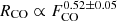 (see also Sanchis et al. 2021). Observing fluxes instead of sizes is less time consuming, firstly, because one would aim to detect, but not necessarily resolve, a target, and secondly, because there would be no need for very deep surveys targeting the faint outer disc regions that contribute marginally to the disc brightness. In this Letter we introduce a simple semi-analytical prescription to compute 12CO disc fluxes under the optically thick assumption. We benchmark this prescription against a grid of full radiative transfer simulations and show that they agree, on average, within a factor of three. Then, as a proof of concept, we compare these models with Lupus and Upper Sco data, highlighting the main limitations of the available datasets and the foreseen improvements with future dedicated surveys.
This Letter is organised as follows. In Sect. 2 we introduce our semi-analytical method. In Sect. 3 we run a disc population synthesis model and compare viscous and MHD-wind predictions with Lupus and Upper Sco data. Our results are discussed in Sect. 4, and in Sect. 5 we draw our conclusions. The code developed for this work is publicly available on github1.
2. Methods
Here we summarise our assumptions and final equation to compute CO fluxes (see Appendix A for the full derivation).
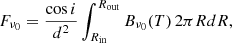
We considered 12CO emission to be optically thick and in local thermodynamical equilibrium. Under these assumptions
 (1)
(1)
where R is the cylindrical disc radius, i the disc inclination, and d its distance from the observer. The brightness profile in Eq. (1) can be written as
 (2)
(2)
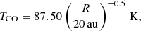
where Bν0 is the black-body emission at temperature T and frequency ν0, and the exponential term gives the thermal broadening of the line (Rybicki & Lightman 1986). Here mCO is the 12CO molecular mass, c the speed of light, and kB the Boltzmann constant. We adopted a power-law temperature profile with exponent −0.5 and normalisation 87.5 K at 20 au, in agreement with the inferences of Law et al. (2021, 2022a,b). Our disc inclination was fixed to the sky-averaged value of cos i = π/4.
We adopted Rin = 10−2 au and Rout = RCO, the radius where the gas surface density equals the column density, NCO = 5 × 1015 cm−2 (a density slightly larger than the standard result of van Dishoeck & Black 1988), where 12CO is not efficiently self-shielded against photodissociation and is quickly removed from the gas phase. To compute the gas surface density corresponding to NCO, we assumed the same carbon abundance of the diffuse ISM, xCO = 10−4. Although it is rather crude, this method is supported by the work of Trapman et al. (2019), who showed that RCO encloses all of the CO emission and is in good agreement with the results of complex thermochemical models. To test our method, we benchmarked our sizes and fluxes against the results of the thermochemical models of Miotello et al. (2016) and Trapman et al. (2020, 2022), run using the code DALI (Bruderer et al. 2012; Bruderer 2013). The results of this exercise are extensively discussed in Appendix B, where we show that our face-on fluxes underestimate DALI ones by a factor of three.
3. Population synthesis
We give a proof of concept of this new method comparing our semi-analytical predictions with the available Lupus (age ≲3 Myr, Luhman & Esplin 2020) and Upper Sco (age 5–10 Myr, Luhman 2020) data. A quick description of the datasets can be found in Appendix C. Here we note that even with the limited data available, working with fluxes instead of sizes increases the samples by a factor of 1.3 (48 instead of 36 sources) in Lupus and by a substantial factor of 3.6 (32 instead of 9 sources) in Upper Sco. For this comparison we relied on a disc population synthesis approach: we prescribed a set of initial conditions and evolved our models in the viscous or MHD-wind case under the assumption that these two SFRs can be regarded as subsequent evolutionary stages of the same population (i.e., they have the same initial conditions). Unfortunately, these initial conditions are either unknown or very uncertain (e.g., they were inferred neglecting any contribution of dust to disc evolution; Lodato et al. 2017; Tabone et al. 2022b). Future more accurate distributions will allow more reliable comparisons between evolutionary models and data.
3.1. Viscous case
We used the Lynden-Bell & Pringle (1974) analytical solution to compute the CO radius. In this case, the surface density at a given time is a function of the viscous timescale (tacc), initial disc mass (M0), and scale radius (R0). We assumed the viscous timescale to be distributed as log(tacc/yr) = 𝒩(5.8, 1.0), where the notation 𝒩(μ, σ) stands for a Gaussian distribution with mean μ and variance σ2. This distribution was inferred by Lodato et al. (2017) fitting the Lupus data in the Ṁacc − Mdisc plane, under the assumption that viscosity is an increasing function of the disc radius with exponent γ = 1.5. For the initial disc mass distribution we considered log(M0/M⊙) = 𝒩(−2.7, 0.7), similarly to Lodato et al. (2017). Even though young discs are known to be small (Maury et al. 2019; Maret et al. 2020; Tobin et al. 2020), their initial disc size distribution is not well constrained. To take into account possible envelope contributions, we adopted the best fit Rdisc ≈ R0 distribution of 25 Class 0 objects in Orion (VANDAM, Tobin et al. 2020) based on the radiative transfer models of Sheehan et al. (2022), under the assumption that gas and dust are co-located at such young ages: log(R0/au) = 𝒩(1.55, 0.4). Finally, we assumed an age of log(t/yr) = 𝒩(5.9, 0.3) for Lupus (corresponding to our choice of tacc; see Lodato et al. 2017) and 7.5 Myr for Upper Sco.
We checked the αSS (Shakura & Sunyaev 1973) distribution associated with our initial conditions (for a M⊙ star):
 (3)
(3)
Here we considered h to be a power law with exponent 0.25 and normalisation h0 = 0.1 at 10 au, in line with the results of Zhang et al. (2021). Our choices of tacc and R0 give a distribution of log αSS ≈ 𝒩(−2.42, 1.06).
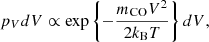
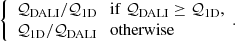
Our results are displayed in Fig. 1. Measured fluxes are shown as purple and orange patches for Lupus and Upper Sco; the survival functions and their 1σ spread were computed using the Kaplan–Meier estimator for left-censored datasets (see Appendix C). The survival functions for Ndiscs = 3000 models are plotted as solid lines of the same colours. Our results under standard assumptions (see Sect. 2) are presented in the left panel. To get a better insight into these flux distributions, we follow the evolution of the median disc (i.e., the disc whose initial conditions are the median of our assumed distributions). This disc spreads viscously, getting bigger and brighter, until an inversion time tinv (Eq. (12) of Toci et al. 2023). Then, the part of the disc that is viscously expanding falls below the CO photodissociation threshold, making the disc smaller and fainter. Our Upper Sco models are fainter than Lupus models because more discs (particularly those with larger R0, lower M0, and shorter tacc) went past their inversion time. Nevertheless, our models are ≳10 times brighter than the data. To reconcile models and observations we introduced a column density fudge factor ξ, that makes photodissociation more efficient: NCO → NCO/ξ. A discussion on the possible physico-chemical interpretation of such a factor can be found in Sect. 4. Our results are displayed in the right panel of Fig. 1, for  and
and  : these fudge factors are able to reconcile models and observations both at the age of Lupus and Upper Sco. However, for the faintest discs in Lupus and the brightest in Upper Sco a smaller (larger) correction factor would be required. This effect can also be due to warmer (colder) discs than our average temperature profile. We note that these fudge factors are not an artefact of our initial conditions; in other words, we found no sensible combination of the initial parameters able to viscously reproduce both Lupus and Upper Sco observations with
 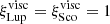 .
.
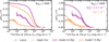 |
Fig. 1. Comparison of the data (patches) and viscous model (solid lines) survival functions at the age of Lupus (purple) and Upper Sco (orange). Left panel: standard assumptions. Right panel: reduced gas column density. Fudge factors (ξvisc, top right corner) are needed to match the data. |
3.2. MHD-wind case
We used the Tabone et al. (2022a) analytical solution with constant magnetic field strength (ω = 1) to compute the CO radius. This solution can reproduce both the disc fraction decay with time and the Lupus data in the Ṁacc − Mdisc plane (Tabone et al. 2022b). In this case the surface density at a given time is a function of the accretion timescale (tacc), the initial disc mass (M0), the initial scale radius (R0), and the lever-arm parameter (λ). Because the wind-driven prescription accounts for disc dispersal after a finite time, knowledge of the disc fraction distribution can be used to infer a distribution of tacc (see Eq. (A.2) of Tabone et al. 2022b). Following Tabone et al. (2022b), our initial disc mass distribution is log-normal with 1.0 dex spread and centred on M0 = 2 × 10⁻³ M⊙, with corresponding mass ejection-to-accretion ratio fM = 0.6. We chose the same initial radius distribution of the viscous case. Then, the lever-arm parameter distribution can be computed from R0 and fM (see Tabone et al. 2022b, where we fixed the innermost wind launching radius to 1 au). The parameter λ is distributed with μ ≈ 4.8 and σ ≈ 0.95. Finally, we assumed an age of 2 Myr for Lupus (corresponding to our choice of M0; see Tabone et al. 2022b) and 7.5 Myr for Upper Sco.
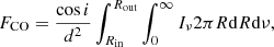
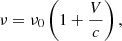
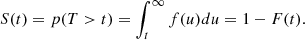
Our results are displayed in the left panel of Fig. 2, using the same symbols as Fig. 1. As noted above, these MHD-wind models have a finite lifetime which was chosen to reproduce the observed age dependence of the disc fraction in SFRs. Since Upper Sco is older than Lupus and their samples are of similar sizes (Appendix C), a larger number of initial discs is needed to reproduce the number of sources observed in the former region: N0, Lup = 196 and N0, Sco = 2490 (in Fig. 2 20 times more models are shown to better explore the initial conditions). In the MHD-wind case the median disc evolves slowly and its radius is constant with time, until t/tdepl ≳ 95%, when fast dispersal takes place and the disc gets abruptly smaller and dimmer. Consequently, we expect our CO flux distributions to be mostly dependent on the initial disc size. A clear difference with the viscous case is that the brightest MHD-wind models are almost as luminous as the brightest Lupus and Upper Sco data, while for fainter and fainter discs the discrepancy between models and data progressively increases. As a consequence, a constant fudge factor cannot reconcile models and observations; a disc mass dependent correction would need to be invoked. We obtained similar results for ω = 0.5 and the initial parameters explored by Tabone et al. (2022b).
 |
Fig. 2. Comparison of the data (patches) and MHD-wind model (solid lines) survival functions at the age of Lupus (purple) and Upper Sco (orange). Left panel: standard assumptions. A mass-dependent depletion factor needs to be invoked to match the data. Right panel: larger initial disc size distribution in Lupus. A constant fudge factor can reproduce the data (dotted line for |

4. Discussion
In this Letter we assumed that the Lupus and Upper Sco disc populations could be considered a respectively younger and older evolutionary stage of the same initial disc population. Under this hypothesis, we ran disc population synthesis models from sensible initial conditions and compared our CO flux distributions with the data.
To match models and data, in the viscous case we introduced a column density fudge factor that increases the CO photodissociation efficiency. This factor can be interpreted as the outcome of some processes depleting CO in protoplanetary discs (Miotello et al. 2022). The low gas masses estimated from CO in Lupus and Chamaeleon I discs (Ansdell et al. 2016, 2018; Miotello et al. 2017; Long et al. 2017) indicate that protoplanetary discs are fainter than expected in CO. This is supported by the few direct measurements of disc masses based on HD rotational line transitions, that require CO to be depleted by factors between 5 and 200 (Bergin et al. 2013; Favre et al. 2013; McClure et al. 2016; Schwarz et al. 2016). Two main processes have been proposed to explain CO underabundance: (i) because of CO chemical (gas- or ice-phase) conversion or evolution, carbon would be sequestered into more complex species, like CO2 or hydrocarbons, that can freeze-out onto grains at higher temperatures than CO (e.g., Bosman et al. 2018; Schwarz et al. 2018; ii) CO freeze-out on dust and subsequent grain growth into larger bodies that no longer participate in gas-phase chemistry would lock carbon up in the disc midplane and transport it radially (e.g., Krijt et al. 2016, 2018; Powell et al. 2022). A combination of the two processes is most likely to take place (e.g., Booth et al. 2017; Krijt et al. 2020) and is needed to explain depletion factors of 100 on a timescale of 1 to 3 Myr inferred from the comparison between Class I and Class II discs (Zhang et al. 2020). The carbon depletion scenario is supported by the detection of C2H in several protoplanetary discs, which can be explained by carbon and oxygen depletion with C/O ≳ 1 (Bergin et al. 2016; Cleeves et al. 2018; Miotello et al. 2019; Bosman et al. 2021). This result is consistent with the carbon-to-oxygen ratio inferred from the available N(CS)/N(SO) upper limits (Semenov et al. 2018; Facchini et al. 2021; Le Gal et al. 2021).
The fudge factor we introduced in the viscous case to explain Lupus data is in line with the observationally inferred CO depletion factors of two orders of magnitude (Miotello et al. 2022). Notably, in addition to CO fluxes, these carbon-depleted models can also reproduce very well the Ṁacc − Mdisc correlation (by construction) and the CO size-luminosity correlation (see Appendix D). Here we caution that our  should be interpreted as a population average rather than an absolute depletion factor; other factors (e.g. a spread in the stellar mass and luminosity, dust evolution, and different source inclinations) can effect CO depletion, either by changing disc chemistry or the observed luminosities. The larger correction needed in the case of Upper Sco, instead, could be explained in three different ways. Firstly, CO is more depleted in Upper Sco than in Lupus. This hypothesis is supported by several evolutionary models, where the carbon depletion factor increases with time (Krijt et al. 2020; Powell et al. 2022). Furthermore, Anderson et al. (2019) showed that CO abundances ≤10−6 are needed to explain the observed N2H+ and CO line fluxes of two Upper Sco discs. Secondly, other processes are affecting disc evolution in Upper Sco. Removing the less bound material from the disc outer regions, external photoevaporation halts viscous spreading, making discs smaller and fainter (e.g., Clarke 2007). While in Lupus the irradiation levels are expected to be low (Cleeves et al. 2016) and photoevaporation to be negligible (with the possible exception of large discs, Haworth et al. 2017), Trapman et al. (2020) argued that the level of irradiation in Upper Sco can be ≈100 times higher and photoevaporation more efficient. Thirdly, the initial conditions are different. In this case, Upper Sco cannot be regarded as the subsequent evolutionary stage of Lupus and the two regions must be modelled separately (e.g., if tacc is shorter in Upper Sco than in Lupus, its disc fluxes will decrease faster).
In the MHD-wind case, models and data have different shapes; no fudge factors are needed to explain the brightest sources, but fainter models require some corrections. Even though Trapman et al. (2022) invoked carbon depletion to reconcile MHD-wind models and the observationally inferred disc sizes in Upper Sco, we note that some of the brightest Upper Sco discs in our dataset were not included in their work because they were not well resolved (see black-contour dots in Fig. C.1). In any case, considering our previous arguments on carbon depletion, our conclusion that MHD-wind models do not need lower CO column densities to match the brightest sources is puzzling. A possible explanation is that our initial disc size distribution is not suitable; in the MHD-wind models of Tabone et al. (2022a,b), R0 is constant with time, and thus it must match the observed disc sizes in Lupus and Upper Sco. For Lupus, assuming as initial disc size distribution log(R0/au) = 𝒩(1.75, 0.4), whose trailing edge agrees with the observationally inferred RCO, 68 distribution (Sanchis et al. 2021), MHD-wind models require a fudge factor of  , similar to the viscous one, to match the data. This is shown in the right panel of Fig. 2, where models with a reduced CO column density are plotted with a dotted line. As in the viscous case, these models can also reproduce very well the Ṁacc − Mdisc correlation (by construction) and the CO size-luminosity correlation (see Appendix D). Instead, the very few constraints on the disc size distribution in Upper Sco are not in contrast with our assumption for the initial disc distribution in Sect. 3. A possible explanation would be that Upper Sco discs were born more compact than Lupus discs (Barenfeld et al. 2016, 2017; Miotello et al. 2021) or became smaller due to environmental effects such as photoevaporation (Trapman et al. 2020). Better data are needed to draw robust conclusions.
5. Conclusions
In this Letter we introduced a new method to study protoplanetary disc evolution based on 12CO fluxes. Assuming optically thick emission, we built a semi-analytical model to compute disc fluxes; the results agree well (within a factor of three) with those of more time-expensive thermochemical models (DALI). Then, we simulated families of discs, evolving from the same initial conditions either under the effect of viscosity or MHD winds, and compared their fluxes with Lupus and Upper Sco data. Using fluxes instead of sizes increases our observational samples by a factor of 1.3 in Lupus and 3.6 in Upper Sco, allowing for a more robust comparisons between models and data.
In the viscous case, our models were brighter than the data. To match the observations, we introduced different column density fudge factors ( and
and  ) that can be explained by carbon depletion (Lupus), and the effects of thermal winds or different initial conditions (Upper Sco). In the MHD-wind case our models matched the brightest discs in Lupus and Upper Sco, but mass-dependent factors were needed to reproduce the fainter sources. In the case of Lupus, when larger initial disc sizes (compatible with the observed distribution) were prescribed, a constant factor (
 , comparable with
  ) was needed to reproduce the observed fluxes.
Unfortunately, our interpretation of the data is limited by the uncertainties on the initial conditions and the amount of carbon depletion. Nevertheless, our proof of concept shows the usefulness of CO fluxes to study disc evolution. Measuring fluxes instead of sizes is less time-consuming. Additionally, fluxes could be the only accessible observable in farther SFRs. Thanks to forthcoming surveys that will target tens of discs at limited resolution and with the potential to inform us about carbon depletion, we will be able to obtain the most knowledge about disc evolution from this new flux-oriented approach.
Acknowledgments
We are grateful to the referee for their useful comments. This Letter makes use of the following ALMA data: for Lupus ADS/JAO.ALMA#2015.1.00222.S (PI J. P. Williams), 2016.1.01239.S (PI S. van Terwisga), 2013.1.00226.S (PI K. Öberg), 2013.1.01020.S (PI T. Tsukagoshi) and for Upper Sco ADS/JAO.ALMA#2011.0.00526.S, 2013.1.00395.S (PI J. Carpenter), 2012.1.00743.S (PI G. van der Plas). ALMA is a partnership of ESO (representing its member states), NSF (USA), and NINS (Japan), together with NRC (Canada), NSC and ASIAA (Taiwan), and KASI (Republic of Korea), in cooperation with the Republic of Chile. The Joint ALMA Observatory is operated by ESO, AUI/NRAO, and NAOJ. We are grateful to L. Trapman for sharing the outputs of his DALI simulations and G. Rosotti for insightful discussions. F.Z. acknowledges support from STFC and Cambridge Trust for a Ph.D. studentship and is grateful to ESO for hosting him for the 2019 Summer Research Programme (Manara et al. 2019) and the 2022 Visitor Programme, when most of this work came to life. S.F. is funded by the European Union under the European Union’s Horizon Europe Research & Innovation Programme 101076613 (UNVEIL). A.M. acknowledges the Deutsche Forschungsgemeinschaft (DFG, German Research Foundation) – Ref no. FOR 2634/2, ER685/11-1. C.F.M. is funded by the European Union under the European Union’s Horizon Europe Research & Innovation Programme 101039452 (WANDA). Views and opinions expressed are however those of the author(s) only and do not necessarily reflect those of the European Union or the European Research Council. Neither the European Union nor the granting authority can be held responsible for them. This project has received funding from the European Union’s Horizon 2020 research and innovation programme under the Marie Sklodowska-Curie grant agreement No 823823 (Dustbusters RISE project). Software: numpy (Harris et al. 2020), matplotlib (Hunter 2007), scipy (Virtanen et al. 2020), JupyterNotebook (Kluyver et al. 2016), lifelines (Davidson-Pilon 2019).
References
- Anderson, D. E., Blake, G. A., Bergin, E. A., et al. 2019, ApJ, 881, 127 [Google Scholar]
- Ansdell, M., Williams, J. P., van der Marel, N., et al. 2016, ApJ, 828, 46 [Google Scholar]
- Ansdell, M., Williams, J. P., Trapman, L., et al. 2018, ApJ, 859, 21 [NASA ADS] [CrossRef] [Google Scholar]
- Barenfeld, S. A., Carpenter, J. M., Ricci, L., & Isella, A. 2016, ApJ, 827, 142 [Google Scholar]
- Barenfeld, S. A., Carpenter, J. M., Sargent, A. I., Isella, A., & Ricci, L. 2017, ApJ, 851, 85 [Google Scholar]
- Bergin, E. A., Cleeves, L. I., Gorti, U., et al. 2013, Nature, 493, 644 [Google Scholar]
- Bergin, E. A., Du, F., Cleeves, L. I., et al. 2016, ApJ, 831, 101 [Google Scholar]
- Blandford, R. D., & Payne, D. G. 1982, MNRAS, 199, 883 [CrossRef] [Google Scholar]
- Booth, R. A., Clarke, C. J., Madhusudhan, N., & Ilee, J. D. 2017, MNRAS, 469, 3994 [Google Scholar]
- Bosman, A. D., Walsh, C., & van Dishoeck, E. F. 2018, A&A, 618, A182 [NASA ADS] [CrossRef] [EDP Sciences] [Google Scholar]
- Bosman, A. D., Alarcón, F., Bergin, E. A., et al. 2021, ApJS, 257, 7 [NASA ADS] [CrossRef] [Google Scholar]
- Bruderer, S. 2013, A&A, 559, A46 [NASA ADS] [CrossRef] [EDP Sciences] [Google Scholar]
- Bruderer, S., van Dishoeck, E. F., Doty, S. D., & Herczeg, G. J. 2012, A&A, 541, A91 [NASA ADS] [CrossRef] [EDP Sciences] [Google Scholar]
- Canovas, H., Caceres, C., Schreiber, M. R., et al. 2016, MNRAS, 458, L29 [CrossRef] [Google Scholar]
- Cazzoletti, P., Manara, C. F., Liu, H. B., et al. 2019, A&A, 626, A11 [NASA ADS] [CrossRef] [EDP Sciences] [Google Scholar]
- Cieza, L. A., Ruíz-Rodríguez, D., Hales, A., et al. 2019, MNRAS, 482, 698 [Google Scholar]
- Clarke, C. J. 2007, MNRAS, 376, 1350 [NASA ADS] [CrossRef] [Google Scholar]
- Cleeves, L. I., Öberg, K. I., Wilner, D. J., et al. 2016, ApJ, 832, 110 [Google Scholar]
- Cleeves, L. I., Öberg, K. I., Wilner, D. J., et al. 2018, ApJ, 865, 155 [Google Scholar]
- Davidson-Pilon, C. 2019, J. Open Source Softw., 4, 1317 [NASA ADS] [CrossRef] [Google Scholar]
- Facchini, S., Teague, R., Bae, J., et al. 2021, AJ, 162, 99 [NASA ADS] [CrossRef] [Google Scholar]
- Favre, C., Cleeves, L. I., Bergin, E. A., Qi, C., & Blake, G. A. 2013, ApJ, 776, L38 [Google Scholar]
- Harris, C. R., Millman, K. J., van der Walt, S. J., et al. 2020, Nature, 585, 357 [NASA ADS] [CrossRef] [Google Scholar]
- Haworth, T. J., Facchini, S., Clarke, C. J., & Cleeves, L. I. 2017, MNRAS, 468, L108 [CrossRef] [Google Scholar]
- Hunter, J. D. 2007, Comput. Sci. Eng., 9, 90 [NASA ADS] [CrossRef] [Google Scholar]
- Kluyver, T., Ragan-Kelley, B., Pérez, F., et al. 2016, in Positioning and Power in Academic Publishing: Players, Agents and Agendas, eds. F. Loizides, & B. Scmidt (IOS Press), 87 [Google Scholar]
- Krijt, S., Ciesla, F. J., & Bergin, E. A. 2016, ApJ, 833, 285 [Google Scholar]
- Krijt, S., Schwarz, K. R., Bergin, E. A., & Ciesla, F. J. 2018, ApJ, 864, 78 [Google Scholar]
- Krijt, S., Bosman, A. D., Zhang, K., et al. 2020, ApJ, 899, 134 [NASA ADS] [CrossRef] [Google Scholar]
- Law, C. J., Teague, R., Loomis, R. A., et al. 2021, ApJS, 257, 4 [NASA ADS] [CrossRef] [Google Scholar]
- Law, C. J., Crystian, S., Teague, R., et al. 2022a, ApJ, 932, 114 [NASA ADS] [CrossRef] [Google Scholar]
- Law, C. J., Teague, R., Öberg, K. I., et al. 2022b, ApJ, submitted [arXiv:2212.08667] [Google Scholar]
- Le Gal, R., Öberg, K. I., Teague, R., et al. 2021, ApJS, 257, 12 [NASA ADS] [CrossRef] [Google Scholar]
- Lodato, G., Scardoni, C. E., Manara, C. F., & Testi, L. 2017, MNRAS, 472, 4700 [NASA ADS] [CrossRef] [Google Scholar]
- Long, F., Herczeg, G. J., Pascucci, I., et al. 2017, ApJ, 844, 99 [Google Scholar]
- Long, F., Andrews, S. M., Rosotti, G., et al. 2022, ApJ, 931, 6 [NASA ADS] [CrossRef] [Google Scholar]
- Luhman, K. L. 2020, AJ, 160, 186 [NASA ADS] [CrossRef] [Google Scholar]
- Luhman, K. L., & Esplin, T. L. 2020, AJ, 160, 44 [Google Scholar]
- Lynden-Bell, D., & Pringle, J. E. 1974, MNRAS, 168, 603 [Google Scholar]
- Manara, C. F., Harrison, C., Zanella, A., et al. 2019, The Messenger, 178, 57 [NASA ADS] [Google Scholar]
- Manara, C. F., Ansdell, M., Rosotti, G. P., et al. 2022, ArXiv e-prints [arXiv:2203.09930] [Google Scholar]
- Maret, S., Maury, A. J., Belloche, A., et al. 2020, A&A, 635, A15 [NASA ADS] [CrossRef] [EDP Sciences] [Google Scholar]
- Maury, A. J., André, P., Testi, L., et al. 2019, A&A, 621, A76 [NASA ADS] [CrossRef] [EDP Sciences] [Google Scholar]
- McClure, M. K., Bergin, E. A., Cleeves, L. I., et al. 2016, ApJ, 831, 167 [Google Scholar]
- Miotello, A., van Dishoeck, E. F., Kama, M., & Bruderer, S. 2016, A&A, 594, A85 [NASA ADS] [CrossRef] [EDP Sciences] [Google Scholar]
- Miotello, A., van Dishoeck, E. F., Williams, J. P., et al. 2017, A&A, 599, A113 [NASA ADS] [CrossRef] [EDP Sciences] [Google Scholar]
- Miotello, A., Facchini, S., van Dishoeck, E. F., et al. 2019, A&A, 631, A69 [NASA ADS] [CrossRef] [EDP Sciences] [Google Scholar]
- Miotello, A., Rosotti, G., Ansdell, M., et al. 2021, A&A, 651, A48 [NASA ADS] [CrossRef] [EDP Sciences] [Google Scholar]
- Miotello, A., Kamp, I., Birnstiel, T., Cleeves, L. I., & Kataoka, A. 2022, ArXiv e-prints [arXiv:2203.09818] [Google Scholar]
- Najita, J. R., & Bergin, E. A. 2018, ApJ, 864, 168 [Google Scholar]
- Pascucci, I., Testi, L., Herczeg, G. J., et al. 2016, ApJ, 831, 125 [Google Scholar]
- Pascucci, I., Cabrit, S., Edwards, S., et al. 2022, ArXiv e-prints [arXiv:2203.10068] [Google Scholar]
- Powell, D., Gao, P., Murray-Clay, R., & Zhang, X. 2022, Nat. Astron., 6, 1147 [CrossRef] [Google Scholar]
- Rosotti, G. P., Tazzari, M., Booth, R. A., et al. 2019, MNRAS, 486, 4829 [NASA ADS] [CrossRef] [Google Scholar]
- Rybicki, G. B., & Lightman, A. P. 1986, Radiative Processes in Astrophysics (Wiley-VCH) [Google Scholar]
- Sanchis, E., Testi, L., Natta, A., et al. 2020, A&A, 633, A114 [NASA ADS] [CrossRef] [EDP Sciences] [Google Scholar]
- Sanchis, E., Testi, L., Natta, A., et al. 2021, A&A, 649, A19 [NASA ADS] [CrossRef] [EDP Sciences] [Google Scholar]
- Schwarz, K. R., Bergin, E. A., Cleeves, L. I., et al. 2016, ApJ, 823, 91 [CrossRef] [Google Scholar]
- Schwarz, K. R., Bergin, E. A., Cleeves, L. I., et al. 2018, ApJ, 856, 85 [Google Scholar]
- Semenov, D., Favre, C., Fedele, D., et al. 2018, A&A, 617, A28 [NASA ADS] [CrossRef] [EDP Sciences] [Google Scholar]
- Shakura, N. I., & Sunyaev, R. A. 1973, A&A, 24, 337 [NASA ADS] [Google Scholar]
- Sheehan, P. D., Tobin, J. J., Looney, L. W., & Megeath, S. T. 2022, ApJ, 929, 76 [NASA ADS] [CrossRef] [Google Scholar]
- Tabone, B., Rosotti, G. P., Cridland, A. J., Armitage, P. J., & Lodato, G. 2022a, MNRAS, 512, 2290 [NASA ADS] [CrossRef] [Google Scholar]
- Tabone, B., Rosotti, G. P., Lodato, G., et al. 2022b, MNRAS, 512, L74 [NASA ADS] [CrossRef] [Google Scholar]
- Tobin, J. J., Sheehan, P. D., Megeath, S. T., et al. 2020, ApJ, 890, 130 [CrossRef] [Google Scholar]
- Toci, C., Rosotti, G., Lodato, G., Testi, L., & Trapman, L. 2021, MNRAS, 507, 818 [NASA ADS] [CrossRef] [Google Scholar]
- Toci, C., Lodato, G., Livio, F. G., Rosotti, G., & Trapman, L. 2023, MNRAS, 518, L69 [Google Scholar]
- Trapman, L., Facchini, S., Hogerheijde, M. R., van Dishoeck, E. F., & Bruderer, S. 2019, A&A, 629, A79 [NASA ADS] [CrossRef] [EDP Sciences] [Google Scholar]
- Trapman, L., Rosotti, G., Bosman, A. D., Hogerheijde, M. R., & van Dishoeck, E. F. 2020, A&A, 640, A5 [EDP Sciences] [Google Scholar]
- Trapman, L., Tabone, B., Rosotti, G., & Zhang, K. 2022, ApJ, 926, 61 [NASA ADS] [CrossRef] [Google Scholar]
- van der Plas, G., Ménard, F., Ward-Duong, K., et al. 2016, ApJ, 819, 102 [NASA ADS] [CrossRef] [Google Scholar]
- van Dishoeck, E. F., & Black, J. H. 1988, ApJ, 334, 771 [Google Scholar]
- van Terwisga, S. E., van Dishoeck, E. F., Ansdell, M., et al. 2018, A&A, 616, A88 [NASA ADS] [CrossRef] [EDP Sciences] [Google Scholar]
- Virtanen, P., Gommers, R., Oliphant, T. E., et al. 2020, Nat. Methods, 17, 261 [Google Scholar]
- Zagaria, F., Rosotti, G. P., Clarke, C. J., & Tabone, B. 2022, MNRAS, 514, 1088 [CrossRef] [Google Scholar]
- Zhang, K., Schwarz, K. R., & Bergin, E. A. 2020, ApJ, 891, L17 [Google Scholar]
- Zhang, K., Booth, A. S., Law, C. J., et al. 2021, ApJS, 257, 5 [NASA ADS] [CrossRef] [Google Scholar]
- Zormpas, A., Birnstiel, T., Rosotti, G. P., & Andrews, S. M. 2022, A&A, 661, A66 [NASA ADS] [CrossRef] [EDP Sciences] [Google Scholar]
Appendix A: Model derivation
Under the assumptions that the 12CO emission is optically thick and in local thermodynamical equilibrium (LTE), the CO brightness at the emitting frequency ν0 can be computed as
 (A.1)
(A.1)
where Bν0 is the black-body emission at temperature T, R is the disc cylindrical radius, i is its inclination, and d is the distance from the observer. We adopted a temperature profile similar to those inferred from CO high-resolution and sensitivity data in T Tauri discs (Law et al. 2021, 2022a,b),
 (A.2)
(A.2)
and added a temperature floor of Tfloor = 7 K, the typical interstellar radiation field in low-mass SFRs:
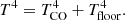 (A.3)
(A.3)
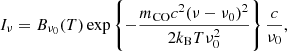
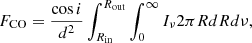
A comparison of our temperature profile in Eq. A.2 and those of Law et al. (2021, 2022a,b) is shown in Fig. A.1.
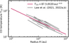 |
Fig. A.1. Comparison between Eq. A.2 (purple line) and the observationally inferred CO temperature profiles (grey). Data: IM Lup, AS 209, and GM Aur by Law et al. (2021); MY Lup, GW Lup, WaOph 6, DoAr 25, Sz 91, and CI Tau by Law et al. (2022a); DM Tau and LkCa 15 by Law et al. (2022b). |
We took into account thermal broadening of the 12CO line as explained by Rybicki & Lightman (1986). Calling V the gas velocity component along the line of sight, the probability of a CO molecule to be in the velocity range between V and V + dV follows the Maxwell–Boltzmann distribution
 (A.4)
(A.4)
where mCO is the 12CO molecular mass, c the speed of light, and kB the Boltzmann constant. The change in frequency (Doppler shift) associated with the velocity V is
 (A.5)
(A.5)
and hence, because pνdν = pVdV,
![Mathematical equation: $$ \begin{aligned} p_\nu d\nu =\dfrac{dV}{d\nu }p_V\left[\dfrac{c(\nu -\nu _0)}{\nu _0}\right]d\nu =\dfrac{c}{\nu _0}p_V\left[\dfrac{c(\nu -\nu _0)}{\nu _0}\right]d\nu . \end{aligned} $$](/articles/aa/full_html/2023/04/aa46164-23/aa46164-23-eq20.gif) (A.6)
(A.6)
Combining this expression with Eq. A.1 and integrating over the velocity space gives
 (A.7)
(A.7)
with
 (A.8)
(A.8)
which implicitly assumes that optical depth affects the line profile only at the peak (i.e. that the line is not optically thick on a wide velocity range), otherwise its profile would be saturated. The inclination was fixed to the sky-averaged value of cos i = π/4, and we adopted Rin = 10−2 au and Rout = RCO, the photodissociation radius (see Sect. 2).
Appendix B: Comparison with DALI models
We benchmarked the results of our semi-analytical model against the disc sizes and fluxes from the thermochemical radiative transfer code DALI published by Trapman et al. (2020, 2022) and Miotello et al. (2016) in the viscous and MHD-wind case, and for different disc inclinations, respectively. We considered a standard diffuse ISM carbon abundance, xCO = 10−4, and a photodissociation threshold of NCO = 5 × 1015 cm−2. Even though, this value is higher than the standard photodissociation column density of van Dishoeck & Black (1988), it gives a better agreement between disc sizes in DALI and our model. We tentatively attribute this difference to the effects of freeze-out on the CO column density in DALI.
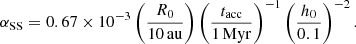
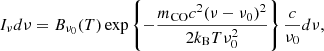
In the viscous case, sizes and fluxes are from the models of Trapman et al. (2020) for different initial disc masses and viscous timescales (see Table 1 therein), R0 = 10 au, d = 150 pc, and cos i = 1. Previous to comparison we converted the 90% CO sizes of Trapman et al. (2020) to RCO using Eq. F.7 in Trapman et al. (2019) and a power-law temperature profile of 40 K at 20 au and −0.25 exponent. For a given quantity 𝒬 ∈ {RCO, FCO} we computed the discrepancy factor between thermochemical model (𝒬DALI) and our method (𝒬1D) results as
 (B.1)
(B.1)
Our discrepancy factors are shown in the upper and lower panels of Fig. B.1 for sizes and fluxes. We used a colour gradient for different disc viscosities and the upward or downward triangle when DALI results overestimate or underestimate ours (Eq. B.1). Clearly, our models overestimate DALI disc sizes by less than a factor 1.3 in most cases and underestimate DALI fluxes by less than a factor 2.5. This difference is due to differences in the line profile because of the high optical depth.
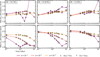 |
Fig. B.1. Discrepancy factor (Eq. B.1) between the 12CO J = 2 − 1 sizes (upper panels) and fluxes (lower panels) from our semi-analytical model and DALI (from Trapman et al. 2020) as a function of time, for a different disc mass and viscous timescale. Upward and downward triangles are used when DALI fluxes overestimate or underestimate our model fluxes, respectively. |
In the MHD-wind case, sizes and fluxes are from Trapman et al. (2022) for different initial disc masses, tacc = 0.5 Myr, R0 = 65 au, λ = 3, d = 150 pc, and cos i = 1. Our discrepancy factors are shown in Fig. B.2. Sizes agree well within a factor of 1.75 and fluxes within a factor of two in most cases.
 |
Fig. B.2. Discrepancy factor (Eq. B.1) between the 12CO J = 2 − 1 sizes (right panels) and fluxes (left panels) from our semi-analytical model and DALI (from Trapman et al. 2022) as a function of time, for a different disc mass. Upward and downward triangles are used when DALI fluxes overestimate or underestimate our model fluxes, respectively. |
As a final test, we compared our model fluxes with those of Miotello et al. (2016) for different disc inclinations. In this case we adopted a truncated power-law density profile with decay exponent γ = 1.5 (Lynden-Bell & Pringle 1974), on a log-spaced grid with 1 ≤ log(R/au)≤4 and a distance of 100 pc (Miotello et al. 2016). Our results are shown in Fig. B.3, where the discrepancy factor is plotted as a function of the disc mass for a different scale radius for the 12CO J = 2 − 1 transition at 230.538 GHz. We used purple and yellow symbols for different disc inclinations (10 and 80 degrees, respectively) and the upward or downward triangle when DALI fluxes overestimate or underestimate our model fluxes (Eq. B.1).
 |
Fig. B.3. Discrepancy factor (Eq. B.1) between the 12CO J = 2 − 1 fluxes from our semi-analytical model and DALI (from Miotello et al. 2016) as a function of the disc mass, for a different scale radius and disc inclination. Upward and downward triangles are used when DALI fluxes overestimate or underestimate our model fluxes, respectively. |
For models close to face-on (i = 10°), we recover a good agreement between the 1D model and DALI fluxes, with a discrepancy factor of less than two. Instead, for models close to edge-on (i = 80°), DALI fluxes are larger than ours by a factor of four to six. This can be explained by the increased optical depth through the line of sight, which makes the (otherwise optically thin) outer disc regions more opaque, increasing DALI model fluxes. In Fig. B.3, very large and massive discs (R0 = 200 au, M0 ≥ 5 × 10⁻³ M⊙) have a different behaviour, that can be explained by the effects of freeze-out, included in DALI but not in our models. The more massive a disc is, the less efficiently the stellar radiation can penetrate its atmosphere and heat its mid-plane (Miotello et al. 2016); this can cause high-levels of CO freeze-out that make the disc fainter. Larger discs are more prone to freeze-out because more mass resides in the colder outer regions. Even though the optical depth and temperature effects can be taken into account parametrically (e.g. Toci et al. 2023, for freeze-out), we decided to keep our model as simple as possible. This is motivated by Fig. B.4, where some of our viscous models from Sect. 3 are plotted over the average DALI discrepancy factor. Most of our models fall in a region of the parameter space where the discrepancy factor is about three.
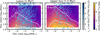 |
Fig. B.4. Comparison between the background average discrepancy factor between 1D models and the DALI fluxes of Miotello et al. (2016) (Eq. B.1) and the disc population synthesis models, colour-coded by their CO flux, in the same disc mass and scale radius range. Most models are expected to reproduce DALI fluxes within a factor of three. |
We obtained very similar results in the case of the 12CO J = 3 − 2 transition at 345.796 GHz.
Appendix C: Sample description
In this section we briefly introduce the Lupus and Upper Sco samples taken into account in Sect. 3.
Lupus discs were observed with ALMA in different programs (Ansdell et al. 2018; van Terwisga et al. 2018; Cleeves et al. 2016; Canovas et al. 2016; Sanchis et al. 2020, see summary in Table 1 of Sanchis et al. 2021) targeting a total of 100 discs. We have no information on CO fluxes for the five brown-dwarf discs observed by Sanchis et al. (2020). Of the remaining 95 discs, 48 were detected (>3σ, Ansdell et al. 2018) and 36 resolved (Sanchis et al. 2021) in 12CO. Upper Sco discs were observed with ALMA in different programs (Barenfeld et al. 2016; van der Plas et al. 2016) targeting a total of 113 discs. Of these, 32 were detected (>3σ, Barenfeld et al. 2016; van der Plas et al. 2016) and 9 resolved (with well-constrained sizes, Barenfeld et al. 2017; Trapman et al. 2020) in 12CO. It is then already clear that considering fluxes instead of sizes increases the sample by a factor of 1.3 in Lupus and by a remarkable 3.6 in Upper Sco. We further note that in Lupus the unresolved discs are all among the faintest sources, while in Upper Sco there are some unresolved discs that are brighter (and potentially larger) than the largest resolved ones. The Lupus surveys targeted the 12CO J = 2 − 1 transition, and the Upper Sco surveys observed the J = 3 − 2 transition. To get a homogeneous sample, we rescaled the CO fluxes to the J = 2 − 1 rest frequency multiplying by the square of the ratio of the J = 2 − 1 to J = 3 − 2 frequencies, assuming that the Rayleigh-Jeans approximation holds. We checked this assumption for our models and it works well with marginal discrepancies for the largest discs, where the temperatures can be low in the outer regions. We also rescaled the fluxes to a common distance of 150 pc using the Gaia EDR3 distances provided by Manara et al. (2022).
To compare models and observations we made use of the survival function. For a real-valued random variable T, known as lifetime, with probability density function f and cumulative distribution function F, the survival function S is defined as
 (C.1)
(C.1)
For the observational samples, the survival functions were computed considering the CO flux upper limits (left-censored dataset) using the Kaplan-Mayer estimator built in the Python package lifelines (Davidson-Pilon 2019) and are shown in Fig. C.1 in purple and orange for Lupus and Upper Sco. Resolved discs (Barenfeld et al. 2017; Sanchis et al. 2021) are plotted with a black contour.
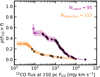 |
Fig. C.1. Survival function for Lupus (purple) and Upper Sco (orange). The number of discs targeted by ALMA in each SFR is shown in the same colour in the upper right corner. Resolved discs are plotted with a black contour. |
We would like to highlight two notes of caution. Firstly, while the Lupus sample is complete (i.e. all young stars with Class II or flat IR excess were observed with ALMA), Upper Sco is not (Luhman & Esplin 2020), which makes the survival function normalisation and the comparison between models and data (see Sect. 3) more uncertain. Future surveys observing a larger fraction of Upper Sco stars with discs will make this comparison more reliable. Secondly, a non-negligible fraction of Lupus discs (≥17, splitting equally between detections, 10, and non-detections, 7) are affected by foreground absorption. Instead, Barenfeld et al. (2016) do not report any information on foreground absorption in Upper Sco. For this reason we decided not to take it into account in our analysis.
Appendix D: Comparison with the size–luminosity correlation
Sanchis et al. (2021) and Long et al. (2022) showed that for the few sources with well-resolved 12CO emission, fluxes and sizes are correlated. In Fig. D.1 our best fit viscous and MHD-wind models from Sect. 3 (blue and green dots) are plotted in the size–luminosity plane in comparison with Long et al. (2022) data (orange dots), excluding TW Hya and the Herbig discs. Our models reproduce well the correlation slope and normalisation: they are roughly 1.5 times fainter than the bulk of the data, consistent with the systematic underestimation of our fluxes by a factor of two to three when compared to DALI models. The scatter about the correlation, instead, is underestimated. A better agreement could be obtained introducing a dispersion, for example in the CO temperature (as in Fig. A.1), which is expected to depend on the stellar luminosity and potentially the disc age.
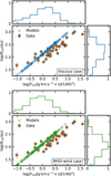 |
Fig. D.1. CO size–luminosity correlation. Data are plotted as orange dots and models as blue (viscous case, upper panel) and green (MHD-wind case, bottom panel) dots. Both models can reproduce the correlation slope and roughly its normalisation. |
All Figures
|
Fig. 1. Comparison of the data (patches) and viscous model (solid lines) survival functions at the age of Lupus (purple) and Upper Sco (orange). Left panel: standard assumptions. Right panel: reduced gas column density. Fudge factors (ξvisc, top right corner) are needed to match the data. |
| In the text | |
|
Fig. 2. Comparison of the data (patches) and MHD-wind model (solid lines) survival functions at the age of Lupus (purple) and Upper Sco (orange). Left panel: standard assumptions. A mass-dependent depletion factor needs to be invoked to match the data. Right panel: larger initial disc size distribution in Lupus. A constant fudge factor can reproduce the data (dotted line for |
| In the text | |
|
Fig. A.1. Comparison between Eq. A.2 (purple line) and the observationally inferred CO temperature profiles (grey). Data: IM Lup, AS 209, and GM Aur by Law et al. (2021); MY Lup, GW Lup, WaOph 6, DoAr 25, Sz 91, and CI Tau by Law et al. (2022a); DM Tau and LkCa 15 by Law et al. (2022b). |
| In the text | |
|
Fig. B.1. Discrepancy factor (Eq. B.1) between the 12CO J = 2 − 1 sizes (upper panels) and fluxes (lower panels) from our semi-analytical model and DALI (from Trapman et al. 2020) as a function of time, for a different disc mass and viscous timescale. Upward and downward triangles are used when DALI fluxes overestimate or underestimate our model fluxes, respectively. |
| In the text | |
|
Fig. B.2. Discrepancy factor (Eq. B.1) between the 12CO J = 2 − 1 sizes (right panels) and fluxes (left panels) from our semi-analytical model and DALI (from Trapman et al. 2022) as a function of time, for a different disc mass. Upward and downward triangles are used when DALI fluxes overestimate or underestimate our model fluxes, respectively. |
| In the text | |
|
Fig. B.3. Discrepancy factor (Eq. B.1) between the 12CO J = 2 − 1 fluxes from our semi-analytical model and DALI (from Miotello et al. 2016) as a function of the disc mass, for a different scale radius and disc inclination. Upward and downward triangles are used when DALI fluxes overestimate or underestimate our model fluxes, respectively. |
| In the text | |
|
Fig. B.4. Comparison between the background average discrepancy factor between 1D models and the DALI fluxes of Miotello et al. (2016) (Eq. B.1) and the disc population synthesis models, colour-coded by their CO flux, in the same disc mass and scale radius range. Most models are expected to reproduce DALI fluxes within a factor of three. |
| In the text | |
|
Fig. C.1. Survival function for Lupus (purple) and Upper Sco (orange). The number of discs targeted by ALMA in each SFR is shown in the same colour in the upper right corner. Resolved discs are plotted with a black contour. |
| In the text | |
|
Fig. D.1. CO size–luminosity correlation. Data are plotted as orange dots and models as blue (viscous case, upper panel) and green (MHD-wind case, bottom panel) dots. Both models can reproduce the correlation slope and roughly its normalisation. |
| In the text | |
Current usage metrics show cumulative count of Article Views (full-text article views including HTML views, PDF and ePub downloads, according to the available data) and Abstracts Views on Vision4Press platform.
Data correspond to usage on the plateform after 2015. The current usage metrics is available 48-96 hours after online publication and is updated daily on week days.
Initial download of the metrics may take a while.