| Issue |
A&A
Volume 692, December 2024
|
|
|---|---|---|
| Article Number | A192 | |
| Number of page(s) | 31 | |
| Section | Stellar structure and evolution | |
| DOI | https://doi.org/10.1051/0004-6361/202450176 | |
| Published online | 13 December 2024 | |
The rotation rate of single- and double-lined southern O stars
Determining what increases the rotation rate in binaries
1
Ruhr University Bochum, Faculty of Physics and Astronomy, Astronomical Institute (AIRUB), 44780 Bochum, Germany
2
Polish Academy of Sciences, Nicolaus Copernicus Astronomical Center, Bartycka 18, 00-716 Warszawa, Poland
3
Universidad Católica del Norte, Instituto de Astronomía, Avenida Angamos 0610, Antofagasta, Chile
⋆ Corresponding authors; This email address is being protected from spambots. You need JavaScript enabled to view it.
; This email address is being protected from spambots. You need JavaScript enabled to view it.
; This email address is being protected from spambots. You need JavaScript enabled to view it.
Received:
29
March
2024
Accepted:
14
October
2024
Abstract
We determined the projected rotational velocity (v sin i) of 238 southern O stars selected from the Galactic O-star Survey. The sample contains 130 spectroscopic single stars (C), 36 single-lined binaries (SB1), and 72 SB2 systems (including eight triples). We applied the Fourier method to high-resolution spectra taken at Cerro Murphy, Chile, and supplemented by archival spectra. The overall v sin i statistics peaks at slow rotators (40–100 km/s) with a tail towards medium (100–200 km/s) and fast rotators (200–400 km/s). Binaries, on average, show increased rotation, which differs for close (Porb < 10 d) and wide binaries (10 d < Porb < 3700 d), and for primaries and secondaries. The spin-up of close binaries is well explained by the superposition of spin-orbit synchronisation and mass transfer via Roche-lobe overflow. The increased rotation of wide binaries, however, needs another explanation. Therefore, we discuss various spin-up mechanisms. Timescale arguments lead us to favour a scenario where wide O binaries are spun-up by a combination of cloud or disk fragmentation, which lays the basis of triple and multiple stars, and the subsequent merging or swallowing of low-mass by higher-mass stars or proto-stars.
Key words: binaries: spectroscopic / stars: evolution / stars: massive / stars: rotation
© The Authors 2024
 Open Access article, published by EDP Sciences, under the terms of the Creative Commons Attribution License (https://creativecommons.org/licenses/by/4.0), which permits unrestricted use, distribution, and reproduction in any medium, provided the original work is properly cited.
This article is published in open access under the Subscribe to Open model. This email address is being protected from spambots. You need JavaScript enabled to view it. to support open access publication.
1. Introduction
O stars are rare, but are massive and luminous. They strongly influence the evolution of a galaxy. Located near their birth clouds, they trigger the formation of lower mass stars and of the next generation of stars. O stars are the main factories of higher chemical elements blown into the interstellar medium by fast winds and at the end of the stars’ life as a supernova. The initial angular momentum of a cloud core is at least three orders of magnitude larger than the rotational angular momentum of the resulting star and must be redistributed or removed during collapse (Zinnecker & Yorke 2007). The majority of O stars are found in binaries or multiple systems (e.g. Sana et al. 2012; Chini et al. 2012). Then the angular momentum is distributed on the rotational and orbital parts. In a binary the presence of a nearby companion induces tidal forces (Zahn 1975, 1977; Tassoul & Tassoul 1997) as well as mass-exchange and transfer of angular momentum between the primary and the secondary star (Kriz & Harmanec 1975; de Mink et al. 2013, and references therein).
For single O stars in the Milky Way, the projected rotational velocity, veqsin(i) (hereafter v sin i), was derived from the broadening of spectroscopic line profiles (Slettebak 1956; Conti & Ebbets 1977; Penny 1996; Howarth et al. 1997). The line broadening is caused by rotation and turbulence, being disentangled by various techniques (e.g. Simón-Díaz & Herrero 2007, 2014, and references therein). Additional contribution to line broadening comes from stellar pulsations (Aerts et al. 2014) and winds (Howarth & Prinja 1989; Kudritzki & Puls 2000; Martins et al. 2005a). Overall, the v sin i distribution is skewed with a peak at ∼75 km/s and a tail extending to ∼500 km/s. Here we divide the stars along v sin i into three groups: slow, medium, and fast rotators, separated by 100 km/s and 200 km/s.
We define ‘increased rotators’ as medium or fast rotators (v sin i > 100 km/s).
The Galactic O-star Survey (GOS, Maíz-Apellániz et al. 2004; Maíz Apellániz et al. 2016) established a basis to expand v sin i studies to binaries. Sota et al. (2011, 2014) classified the spectral types and binary nature of GOS stars, based on low-resolution (R ∼ 2500) spectra, supplemented by high-resolution information when available. Observationally, large databases of high-resolution spectra are being gathered in the course of several projects. Most prominent are the spectroscopic survey of Galactic OB stars at the IAC (IACOB, PI Sergio Simón Díaz, IAC) and the spectroscopic survey of Galactic O and WN stars (OWN, initiated by Rodolfo Barbá, La Serena). In addition, a dedicated survey on the southern O stars has been performed by our group, aimed at finding eclipsing or spectroscopic binaries, involving photometric and high-resolution spectral monitoring since 2009 from Cerro Murphy1 (PI Rolf Chini, Bochum). Finally, as a low-metallicity starburst complement, the VLT FLAMES Tarantula Survey (VFTS) observed 800 massive stars in the H II region 30 Doradus in the Large Magellanic Cloud (Evans et al. 2011).
Based on the GOS, the IACOB+OWN survey documented the progress in understanding the O stars by dozens of papers. Recently, Holgado et al. (2022) presented a statistical study on the projected rotational velocity (v sin i) of 285 Galactic single-line O stars in the full northern and southern hemisphere. This sample contains 230 single stars ‘C’ with non-detected radial velocity (RV) variations, adopted to have constant RV, and 55 single-lined binaries (SB1) with detected secure RV variations. In the binaries the detected component likely refers to the primary, whereas the secondary is not seen. Compared to the single stars, the primaries show a more pronounced tail of medium rotators, but a deficit of fast rotators. Holgado et al. provide empirical evidence supporting that the tail of fast rotators is mainly produced by binary interactions. Stars with extreme rotation (> 300 km/s) appear as single stars that are located in the lower zone of the spectroscopic Hertzsprung–Russell diagram (sHRD). The rotation rates of the youngest observed stars favour an empirical initial velocity distribution with ≲20% of the critical velocity.
Britavskiy et al. (2023) searched for empirical signatures of binarity in fast-rotating O-type stars (v sin i > 200 km/s). They expanded the IACOB+OWN sample of single-lined O stars (Holgado et al. 2022) by including eight double-lined binaries (SB2) which contain at least one fast rotator (v sin i > 200 km/s). In addition, they imployed Gaia and TESS data for astrometric and photometric (e.g. eclipse) information. Their empirical results seem to be in good agreement with the assumption that the tail of fast-rotating O-type stars is mostly populated by post-interaction binary products.
The VFTS presented v sin i of O stars in the LMC for 216 single stars (Ramírez-Agudelo et al. 2013), 85 SB1s, and 31 SB2s (Ramírez-Agudelo et al. 2015). The overall v sin i distribution of 114 (high-quality) primary stars resembles that of single stars, but it differs in two ways: in binaries the distribution is broader and slightly shifted to higher values. This shift is mostly due to short-period binaries (Porb ≲ 10 d). Second, the v sin i distribution of primaries lacks a significant population of stars spinning faster than 300 km/s, while such a population is clearly present in the single-star sample. The orbital periods were not directly measured, but have been inferred from Monte Carlo simulations of the amplitude of the radial velocity variations, max_dRV, of five to eight epochs (Sana et al. 2013). The higher average spin rate of stars in short-period binaries may either be explained by spin-up through tides in such close binary systems, or by spin-down of a fraction of the presumed-single stars and long-period binaries through magnetic braking (Ramírez-Agudelo et al. 2015). The fraction of SB2s in the VFTS is surprisingly low (31/332 = 9%), only one-third of that found in the Milky Way (Holgado et al. 2022, this work), while that of SB1s is very high (26%), suggesting that the majority of SB2s in the VFTS have escaped detection. Follow-up spectroscopy of 51 SB1s by the Tarantula Massive Binary Monitoring (TMBM) revealed that the SB2 fraction is indeed at least 50% higher (Shenar et al. 2022; Sana et al. 2022).
Comprehensive v sin i statistics of a complete sample of Galactic O stars that includes all SB2s is still desired. In the course of case studies of targeted Galactic clusters and SB2s, the rotation rate of disentangled primaries and secondaries have been derived by various authors using different methods (Table D.2, available at the CDS, lists a compilation of 49 southern SB2s). For this paper we used high-resolution spectra of a GOS-based sample of ∼250 southern O stars monitored with our telescopes from Cerro Murphy and supplemented by archival spectra from FEROS at ESO. We decided to analyse not only the SB2s, but the entire sample in a homogeneous way, to ensure that any methodical biases were minimised. Section 2 lists the sample and the spectra. Section 3 describes the SB classification and the determination of v sin i with the Fourier technique. We used several spectral lines to determine v sin i and checked for consistency. Section 4 presents the v sin i results obtained for different subsamples. In Sect. 5 we discuss the v sin i difference and spin-up mechanisms for close and wide binaries, primaries, and secondaries. Section 6 presents a summary and our conclusions.
2. Sample and spectra
2.1. Sample
We performed a comprehensive spectroscopic survey on a large representative sample of 249 O-type stars south of Declination +20°, visible from Cerro Murphy. Chini et al. (2012) presented early results on the multiplicity.
The sample is drawn from the Galactic O Star Catalogue (GOSC Version 2.0; Sota et al. 2008), which is assumed to be complete to V ≤ 8 mag. Sota et al. (2011, 2014) provided a comprehensive spectral classification. Two stars with four or more components are rejected from the sample, because the lines are faint and it is difficult to obtain reliable v sin i for them; these stars are: HD 101205 (SB7, Zasche et al. 2022), and the multiple system Herschel 36 with no less than 10 stellar components in a radius of 4″ Maíz Apellániz et al. (2015), Campillay et al. (2019). In addition, the complex system HD 57060 (= UW CMa) is excluded: our six spectra show at least three components, two narrow and one broad, with partly eclipses, hindering us to accurately disentangle the components. The O2 supergiant HD 093129 Aab shows at least two components (see also Maíz Apellániz et al. 2017) but unique disentangling of our data was not possible. We therefore rejected this source from the sample. Seven stars with spectral line profiles dominated by extreme winds preventing any reliable v sin i determination are also rejected from the sample: HD 39680, HD 45314, HD 169515, HD 313846, LSS 2063, LSS 4067, and Pismis 24-17. The SB2 system HD 104649 was rejected, because it turned out to be an early B-type pair. HD 93161 AB is now splitted into HD 93161 A and HD 93161 B.
The resulting sample of 238 stars is listed in Tables D.1 and D.2 (available at the CDS), splitted into spectroscopic binary types (C, SB1, SB2 and SB3), newly classified as described in Sect. 3.1. The sample is not strictly complete but it constitutes a representative sample suited for statistical studies, for example on v sin i differences between single- and double-line stars, early- and late-type stars, giants (luminosity class LC I-III) and dwarfs (LC IV+V).
2.2. Spectra
The v sin i study here is based on 3424 high-resolution multi-epoch optical spectra. About half (1762 spectra) were taken with the Bochum Echelle Spectrograph BESO (Fuhrmann et al. 2011) at the Universitätssternwarte Bochum on Cerro Murphy. BESO was mounted at the 1.5 m Hexapod-Telescope in the years from 2009 until 2012 and thereafter until 2020 at the 0.8 m IRIS telescope. BESO is a twin of the ESO FEROS spectrograph (Kaufer et al. 1997, 1999). The spectra comprise a wavelength range from 3620 to 8530 Å with a mean spectral resolution of R = 50 000. The entrance aperture of the star fibre is 3.4 arcsec. The integration time per spectrum was adapted to the published visual brightness of each star. It was our primary goal to monitor a large number of stars rather than to obtain a very high S/N for individual stars. All data were reduced with a pipeline based on the MIDAS package developed for FEROS (Stahl et al. 1999). We complemented the data set with archival high-resolution spectra taken with FEROS at ESO (N = 1628), with UVES at ESO (N = 7) (Dekker et al. 2000), and with ELODIE (N = 28) (Baranne et al. 1996) at the 1.93 m telescope of the Observatoire de Haute-Provence2.
Figure 1 (top) depicts the number of spectra per star; the median is 10 and the minimum is 4 obtained for 3 stars: HD 95589 is a C, BD +22 3782 marginally failed our SB1 criteria (Sect. 3.1) and we assigned C, while HD 93161 B is a robust SB1. Certainly, our SB classification suffers from incompleteness caused in case of small radial velocity differences (dRV), in other words a low mass ratio M2/M1 and/or a large separation of the binary components. This leads to a well-known bias favouring class C as discussed by Sana et al. (2012), among others. Likewise, a faint SB2 companion may escape detection, in particular if it has flat broad lines (e.g. Mahy et al. 2022). The detection of an SB system depends also on the quality of the spectra and their number. The fraction of detected SB systems, fSB, in the sample is about 40–45%. Figure 1 (bottom) compares the number of spectra for Cs and SBs. Cs have on the median about 9/12 fewer spectra than SBs. We note that we have finished the monitoring of a star once the obtained spectra establish its SB nature, even if there are fewer than ten spectra. This may explain the high fraction fSB ≳ 35% for the subsample with only four to ten spectra, in particular if they have been caught by chance at large dRV.
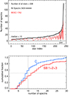 |
Fig. 1. Statistics of the spectra. Top: Number of spectra per star. The star index is sorted in ascending order of the total number of spectra per star (Ntot, black), and for equal Ntot in ascending order of the number of BESO spectra (red). Bottom: Cumulative fraction of the number of spectra for Cs and SBs, zoomed in to the range 0–30. The dotted lines mark the median; Cs have statistically (about 9/12) fewer spectra than SBs. |
3. Analysis
Whenever it was possible, we used the O III 5592 line and in addition suited lines among the master set of He I (4026, 4387, 4471, 4713, 4922, 5876, 6678, 7065) and He II lines (4200, 4541, 4686, 5411). Whether a line is suited depends on several factors and the spectral type of a star: for instance, He I 4387 is too faint in early O-type stars, while O III 5592 and He II lines are absent in B-type companions. He I 5876 is the brightest line but often suffers from wind features. He I 4026, 4387, 6678, 7065 are often noisy in BESO spectra. We took care to reject possible blends which may mimic a binary, e.g. O II 4924.5 near He I 4922, and He II 6683 near He I 6678. In addition, for some objects and spectra the He I 4471 line shows suspicious wings not seen in other helium lines, and in these cases we removed He I 4471 from further analysis. Our aim is to obtain robust v sin i by using as many lines as necessary, rather than using as many lines as possible. After visual inspection, we rejected asymmetric and suspicious cases. Table D.4 (available at the CDS) lists for each line how many stars use the line.
3.1. SB classification
The spectroscopic binary (SB) classification by Chini et al. (2012) was based on a limited number of spectra per star. Now about twice the number of spectra are available, allowing us to improve the former SB classification. Here, we re-inspected all spectra. A number of suspected binaries turn out to be likely single-lined stars with line profile variations (LPV). We have detected two new SB1s (CPD −58 2620, HD 093160) but no new SB2s; in other words: all (except of the two) SB1s and all SB2s found here have meanwhile been reported in publications apart from (Chini et al. 2012). For some SB2s we give the spectral types, if they are not yet published or if they differ from previous works. We here find 135 Cs, 41 SB1s, 54 SB2s and 8 SB3s. The inclusion of literature information yields a sample of 130 Cs, 36 SB1s, 64 SB2s and 8 SB3s for the scientific analysis.
We begin the description with stars with double (triple) lines; they are classified SB2 (SB3) accordingly. We required that the radial velocity (RV) of the binary components is consistent for at least four lines. A varying fast wind may mimic two stellar components with a “false faint secondary” lying in all spectra on the blue side of the line peak. Therefore, as a conservative approach, for an SB2 we required that the secondary should switch the position for different spectral epochs, for example from the blue to the red side of the primary. In addition, the spectral types of the disentangled components, derived from the He I 4471/He II 4541 equivalent width (EW) ratio (Conti & Alschuler 1971; Martins 2018), have to be consistent with literature results. To derive/check the luminosity classes we used the EW ratios He II 4686/He I 4713 and Si IV 4089/He I 4026 (Martins 2018). More details on the disentangling are given in Appendix A.
The stars not classified as SB2 or SB3 are adopted as single line stars. To identify a spectroscopic binary, SB1, it should exhibit reliable dRV. The detectability of RV variations depends on the line width (here denoted as FWHM of the inverted line profile), the line depth (or equivalently EW/FWHM), the signal-to-noise ratio (S/N) of the spectrum and on the number of spectra, whereby some good luck is needed to catch the target at two RVs with a large separation. Based on the experience with our data, in case of good S/N and EW, the uncertainty of RV is about 3% of the FWHM. We determined the FWHM of the line profile and dRVmax, the maximum of dRV for the set of spectra, using the four lines above. In general, the O III 5592 line is the sharpest but has a small EW, while He lines suffer more from LPVs. On the other hand, He I 5876 next to the interstellar lines Na5890 provides low wavelength calibration errors (which are typically about 3 km/s). This way we obtain an SB1 candidate, if dRV > 3 + 0.03 ⋅ FWHM km/s.
The S/N of the spectra is not homogeneous; this holds for both FEROS and BESO spectra as well. In particular, numerous BESO spectra taken during the early HPT operational phase suffer from a poor focus. For our data, the S/N inhomogeneity limits the use of σRV, the RV dispersion. Therefore, all SB1 candidates have been visually inspected by at least two of the three authors independently, and they had to agree on the SB1 classification.
RV variations are easier detected for a star with narrow lines (i.e. small v sin i). This inevitably poses a bias against the detection of SB1s among fast rotators (v sin i > 200 km/s). The remaining stars (not classified as SB1, SB2, SB3) are adopted as C. Nearly all of them show line profile variations (also in O III 5592) which could be real or caused by the relatively large noise. Therefore, we here do not distinguish between C and LPV (as Holgado et al. 2022 did).
3.2. Determination of vsini
3.2.1. Overview and caveats
The broadening of a spectral line profile is essentially caused by the atmospheric turbulence and the stellar rotation (e.g. Slettebak 1956; Conti & Ebbets 1977). It is widely assumed that the line profile Pline can be written as convolution of the stellar rotation profile Prot with the atmospheric turbulence profile Pturb,
 (1)
(1)
where Prot has a round elliptical shape, and Pturb looks more triangular and can be approximated by a Lorentzian profile (or a Gaussian or a combination of both). The different shape “round” and “triangle” has been used to disentangle turbulence and rotation by obtaining a best fit of Eq. (1) to the spectral line (Goodness-Of-Fit method, GOF). Modern techniques use synthetic model spectra for Pturb derived from e.g. the FASTWIND tool (Puls et al. 2005; Rivero González et al. 2012).
The Fourier transform (FT) spectrum of a Lorentzian or Gaussian is featureless, but the FT spectrum of Prot exhibits characteristic minima related to v sin i (Carroll 1933; Gray 1973, 2005), making the FT method ideally suited for determining v sin i. Royer (2005) has successfully applied the FT method to F- and A-type stars. Ryans et al. (2002) and Simón-Díaz & Herrero (2007, 2014) introduced the FT method to single O- and B-type stars and performed a thorough comparison of v sin i derived by FT and GOF. Both methods yield consistent v sin i values. Despite the great success achieved so far, the most important caveat is that other effects than stellar rotation may produce FT minima as well, potentially leading to biased v sin i values.
Conti & Ebbets (1977) already realised a lack of narrow-lined, slow rotating O stars with v sin i ≲ 50 km/s which would be expected for small inclination angles of the rotation axis with respect to the line-of-sight (i < 10°). Indeed, there exist slowly rotating magnetic O stars with well-determined rotation periods implying v sin i ≤ 1 km/s, but both the FT and GOF methods yield v sin i ≈ 45 km/s (Sundqvist et al. 2013). As suggested by these authors and others, the severe v sin i overestimates for slow rotators are most likely caused by an insufficient treatment of the competing broadening mechanisms often referred to as micro- and macro-turbulence. Aerts et al. (2014) also caution the blind application of the FT method to stars with considerable pulsational line broadening. Finally, O-type stars are well known to produce a strong wind (e.g. Howarth & Prinja 1989; Kudritzki & Puls 2000). We suggest that a slow wind (Martins et al. 2005a) or an expanding halo may cause spurious effects on v sin i for slow rotators; we describe some ideas on that in Appendix B. Winds might have only little influence on v sin i for medium and fast rotators which are at the focus of this paper.
3.2.2. Fourier transform method applied here
Compared to Helium and Balmer lines, the metal lines like O III 5592 are well known to be less affected by wind and turbulence, but often weak. Therefore, for each star, we have determined v sin i for O III 5592, several Helium lines. We applied the FT method following the recipes described in Simón-Díaz & Herrero (2007, 2014). We checked that the first FT minimum occurs at a frequency range where the median FT amplitude lies well above the noise level (see Fig. 2 in Simón-Díaz & Herrero 2007); data not fulfilling that criterium are rejected.
Almost all lines show an asymmetric profile. We rejected asymmetric lines where the profile is certainly dominated by a strong wind (P Cyg). Profiles with a mild asymmetry were accepted. Simón-Díaz et al. (2017) have extensively investigated asymmetric profiles and their skewness; profiles with blue or red asymmetries (negative and positive skewness, respectrively) may indicate the presence of stellar oscillations as well.
In order to increase the S/N, we averaged the line profiles from the 2–5 best spectra, shifted for each line to radial velocity RV = 0. We applied the FT method both to single and averaged spectra. The averaged spectra not only show a better S/N but the main advantage is: For the disentangled SB2+SB3 components, averaging the spectra reduces the residual wiggles which arise from a non-perfect disentangling (illustrated in Sect. 3.2.3). Likewise, for pulsating stars the line profile variations may average out.
We found in general that the first FT minimum is shallow, sometimes barely recognisable; this holds in particular for single spectra, where sometimes the first FT minimum escaped detection. Fourier theory predicts that (even small) profile asymmetry may smear out the first FT minimum. To understand the effect of profile asymmetry on the v sin i determination, we artificially symmetrised the profiles (i.e. consider mirrored profiles); we here expand the symmetrising approach of Sundqvist et al. (2013). The mirroring axis has been determined from a parabola fit of the profile trough. This allows us to examine four profile types and derive their v sin i, as illustrated with the example in Fig. 2 (top):
-
(1)
original profile (black dashed)
-
(2)
blue half mirrored (blue)
-
(3)
red half mirrored (red)
-
(4)
averaged red and blue mirrored (green).
The original profile shows a small asymmetry with a blue absorption which likely arises from a slow wind (v < 150 km/s). The three mirrored profiles are symmetric.
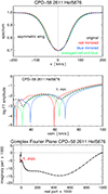 |
Fig. 2. Mirrored asymmetric line profiles and their Fourier transforms. Example from CPD−58°2611 in the He I 5876 line. Top: Original line profile with an asymmetric blue wing (black dashed), as well as the three types of symmetric line profiles: mirroring the red (v > 0 km/s) and blue (v < 0 km/s) halves of the line profile, and in green the averaged mirrored line profile. Middle: FT amplitude of the original line profile (black dashed), and the mirrored profiles (red, blue, green). Bottom: FT of the original asymmetric profile resembles a smooth chain of data points in the complex plane with non-zero imaginary part. The data point of the first minimum of the FT amplitude is marked in red. |
Figure 2 (middle panel) depicts the FT amplitudes: The first FT minimum of the original asymmetric profile (black dashed) is shallow, while the symmetric mirrored profiles yield a sharp minimum (red, blue, green). The green and black FT minima yield essentially the same v sin i values. This gives us confidence that the shallow black minimum is indeed related to the sought-for signature of rotation. However, the red and blue profiles yield smaller and larger v sin i, respectively. This is expected, if the blue profile suffers from the additional line broadening (i.e. the asymmetric wing of the original profile is caused by a wind).
The bottom panel of Fig. 2 plots the FT of the original profile in the complex Fourier plane. Mathematically, the FT of a symmetric profile is real (i.e. the imaginary part is zero). For an asymmetric profile, however, the imaginary part is non-zero; as a consequence the FT data points move in the complex Fourier plane around the (0,0) origin, leading to shallow rather than sharp amplitude minima.
The example of Fig. 2 suggests that the effect of a wind-caused asymmetry may easily be reduced by taking v sin i of the red mirrored profile (see also Sundqvist et al. 2013). However, this strategy seems to be not applicable in general for our data, because negative and positive skewness occur. One reason may be that the skewness is sensitive to the uncertainty of the mirroring axis, in particular for faint noisy lines. Thus, for about half of the lines the red mirrored profile yields a larger v sin i than the blue mirrored profile, contrary to what one would expect, if the blue wing is due to wind.
We take the median of these four v sin i values and the standard deviation of the median as an error estimate (for an individual line, e.g. O III 5592). This way, outliers among the four values have little influence on the adopted v sin i, but a large error warns us that the v sin i calculation may suffer from asymmetric profiles. Indeed, the mirroring method enabled us to reject numerous uncertain cases. Further error considerations are addressed in Sect. 3.2.4.
We were able to determine v sin i for all Cs and SB1s in our sample, and in the 64 SB2 and 8 SB3 systems for all stars except 10 secondaries and 2 tertiaries.
The detection limit for slow v sin i has to be calculated in Fourier space, since we seek for the first minimum of the FT amplitude. The crucial point is not only the spectral resolution (in our case R ∼ 50 000) and the noise level, but also the additional line broadening by turbulence vturb which is strong in O stars (Sect. 2.1. in Simón-Díaz & Herrero 2007). This steepens the decline of the FT amplitude, so that the noise level is reached at larger v sin i, compared to a negligible vturb. We estimate a lower limit of v sin i about 20–30 km/s (consistent with Fig. 4 in Simón-Díaz & Herrero 2007).
3.2.3. Residuals of the disentangling
For SB2s (and SB3s), the Gaussian decomposition may lead to residual wiggles in the resulting line profiles (Appendix A). Mostly the residuals are small, within the noise of the spectra. We have examined possible effects on v sin i, also using simulated line profiles, finding indeed that any effects on the determination of v sin i are negligible. However, a few SB2s show strong residuals, clearly exceeding the noise of the spectra and Fig. 3 shows one of the worst cases, HD 152219 (DT 5). In brief, the take-away messages from the top panels of the figure are:
-
(1)
Residuals can be characterised by Ares/Aline ≳ 0.3, where Ares is the peak-to-peak amplitude of the residual wiggles and Aline is the Gaussian height of the line. Any residuals produced by the faint component (with small Aline) are negligible for the bright component (with large Aline).
-
(2)
Relevant residuals are produced by the bright component (here the primary P) and play a role for the faint component (here the secondary S). Significant effects occur, if Aline(P)/Aline(S) ≳ 3.
-
(3)
Averaging of N spectra with different dRV is able to quickly smooth the residuals. For instance, Ares/Aline of S declines by about N1/2.
-
(4)
If dRV between P and S is sufficiently large, then most of the wiggles lie outside of the line-core of S. Then cutting-out a small window (typically ±3σ) around the line profile of S excludes most of the wiggles.
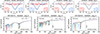 |
Fig. 3. One of the worst cases (DT 5) of the effects of disentangling residuals of HD 152219 in He I 4922. Top, two left panels: Single spectra as observed on 2004 May 09 and on 2006 May 06. The two right panels show the average of the two spectra and of all nine spectra used, whereby each component has been shifted to RV = 0 before averaging. The black lines mark Gaussian fits to the profiles, with FWHM and height Aline labelled. Likewise, the peak-to-peak amplitude of the residual wiggles, Ares, is given, determined outside of the velocity range ±3σ of each profile marked by the coloured vertical bars. Averaging reduces the residual wiggles. Bottom: Fourier transform amplitude of the average of all nine spectra, for the primary (left panel), and for the secondary including and excluding residuals (middle and right panel, respectively). The details are explained in Sect. 3.2.3. |
The bottom row of Fig. 3 depicts the Fourier amplitudes of the average of all 9 spectra used, for the primary (left panel), and for the secondary including and excluding the residuals (middle and right panel), respectively. The four colours refer to the four cases of the mirroring technique (black = original line, red mirrored, blue mirrored and averaged red and blue mirrored). The take-away messages for v sin i are:
-
(5)
The primary is well measured, even with included residuals; excluding the residuals does not change v sin i as expected because they are small and not visible within the noise (FT plot not shown).
-
(6)
v sin i of the secondary changes from 139 ± 4 km/s to 119 ± 2 km/s when the residuals are excluded. The small errors are due to the large symmetry of the profiles. The comparison with FWHM of the line profile (169 km/s, vertical dashed line) strongly supports that the exclusion of the residuals yields a trustable v sin i3.
-
(7)
The quite well-isolated secondary of HD 152219 allows us to estimate a potential v sin i bias of about 20% (factor of 139/119, i.e. ∼1.2), when the residuals are not excluded. In addition, we have explored artificial SB2s using modelled line profiles of rotating stars with turbulence, finding a v sin i bias of typically less than 5% when the residuals are small but reaching up to 20% in worst cases with strong residuals. Such an estimate is useful for binaries where the Gaussian decomposition yields strong residuals for a faint broad secondary. If the secondary is sufficiently broad, then the residuals produced by the primary lie within the line core and cannot be excluded via cutting-out a window. CPD −59 2600 is the worst example of such binaries (see DT 6 in Fig. A.1). Notably, whenever an SB2 in our sample exhibits a bright narrow and a flat broad component, the residuals and the potential v sin i bias only affect the flat component. We checked that the bias does not change the main result, namely that the flat component is significantly broader than the narrow component.
To summarise, we have checked that for our SB2 sample the Gaussian decomposition mostly yields small residuals and negligible effects on v sin i. However, a few cases may suffer from increased uncertainties and a potential bias up to 20%. They do not change the main result qualitatively.
3.2.4. Error estimates
For a given star and a given line (e.g. He I 5876), the mirroring technique yields a formal error (i.e. standard deviation) on v sin i which refers to the symmetry of the line. Often these errors appear unrealistically small, < 5%. For instance, Holgado et al. (2022) found v sin i differences down to ∼10% between the FT method and the Goodness-of-fit method (which we did not apply here). An alternative realistic error may be obtained from the average of v sin i independently measured in several He I lines. Therefore we compared the errors from the two methods: a) from averaging over several lines and b) from the mirroring technique4.
Figure 4 shows the distribution of v sin i errors in percentage, separated for two samples: 148 single-lined stars and 140 stars in SB2+SB3 systems. All stars in SB2+SB3 systems have a v sin i measurement in at least two He I lines, which allows error calculation via method (a). Eighteen of the 166 single-lined stars were omitted in this comparison because they were measured in less than two He I lines. The reason is that these 18 stars show strong winds and P Cyg profiles in most He I lines which were rejected from the v sin i determination. Notably, such sources are not used for the binary disentangling as well, and this likely explains why binaries lack P Cyg profiles in most He I lines, which enables a successful v sin i measurement in these lines. For method (b), the black histograms show the error distribution of the mirroring technique, whereby the number of line measurements (356 and 385, resp.) gives the number of used He I lines integrated over all stars. Basically, for both methods and both samples the error histograms look similar with a peak around 6% and a tail towards 30%. For method (b) the fraction of very small (< 6%) errors is larger. For method (a), choosing a minimum error of 6% may still be optimistic, because v sin i was calculated only for good He I lines (poor lines were excluded from the calculation).
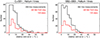 |
Fig. 4. Distribution of v sin i errors in the helium I lines for single-lined stars (left) and for stars in SB2+SB3 systems (right). The width of the histogram bins is 3%. The details are explained in Sect. 3.2.4. |
We conclude that realistic v sin i errors are at least 10%. For the disentangled binaries we have assigned quality flags with a likely v sin i error between 10% and 30% (Appendix A). For both samples, the proposed errors agree also with the differences between literature v sin i values and ours (Sect. 4.2). Furthermore, for slow rotators with v sin i < 100 km/s a minimum error of 10 km/s might be realistic to better account for potential systematic effects.
In this work, we do not use the v sin i errors further but we note that the statistical differences of v sin i (and of line FWHM) between single stars (C) and binaries and between primaries and secondaries are so large that the main results of this paper remain unchanged, even if v sin i errors are taken into account.
4. Results
The large sample allows us to build well-defined subsamples, in order to explore how v sin i depends on the spectral line used, the spectral type, luminosity class, and the SB type.
4.1. v sin i from different spectral lines
For each star we have determined v sin i using several lines with good S/N. In order to compare the statistics of the rotation rate for subsamples (C, SB1, SB2, etc.), we need a “representative” v sin i value for each star. To this end, we used the value from O III (118 C+SB1, 54 stars in SB2+SB3); if O III is not available, then we take the average of He I lines (48 C+SB1, 61 O stars in SB2+SB3, 25 B-type companions). This way we obtain for each star a v sin i value (called bestv sin i) used for the statistical comparison. Table D.3 (available at the CDS) list v sin i for O III and the average of He I lines and of He II lines, and the values for each Helium line5.
The bestv sin i is based on either O III or He I, raising the question on a potential bias. To that end, we sort the stars along rising bestv sin i and then plot for each star the average v sin i values of the lines used (Fig. 5). The horizontal lines mark v sin i ranges, and the corresponding vertical lines visualise the fraction of stars in these ranges. It documents a systematic trend that – for rotators below about 100 km/s – v sin i typically increases from O III over He I to He II lines. This apparent “stratification” disappears for medium and fast rotators, where rotation dominates other line broadening effects. This gives us confidence that for rotators with true v sin i > 150 km/s the bestv sin i is unbiased. On the other hand, for slow rotators with true v sin i < 100 km/s the bestv sin i may depend on whether it is obtained by O III or He I.
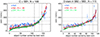 |
Fig. 5. v sin i distribution of different lines. Left for single-lined stars. Right for stars in SB2+SB3 systems, whereby the 25 B-type companions are excluded because their v sin i has been derived solely from He I lines. The legends also list the number of stars with the bestv sin i from O III (green) and He I (red). |
How strong is the effect of a mix of O III and He I based bestv sin i on the comparison between subsamples, e.g. Cs and SB2s? Of particular interest here is the “transition region” around v sin i = 100 km/s between slow and increased (i.e. medium+fast) rotators. Figure 6 compares the v sin i distribution derived from O III and He I, respectively, for stars with measurements in both lines. The results are the following:
-
(1)
The distributions peak at slow v sin i. For He I they shift to slightly larger v sin i than for O III (by less than one histogram bin). The modes of the distributions differ by 6 km/s for single-lined stars and by 10 km/s double-lined stars. The shifts are small, within typical v sin i errors.
-
(2)
When using He I instead of O III, the number (fraction) of stars shifting from slow to increased rotators is 4 out of 107 and 5 out of 54 (i.e. about 4% and 10%) for single- and double-lined stars, respectively. Hence the fractional difference is 6%.
-
(3)
The fraction of stars with He I based bestv sin i is larger for SB2+SB3 than for single-lined stars (61/115 = 53% versus 48/166 ∼ 29%, from Fig. 5). One reason is that O III 5592 is too faint in many double-lined stars and about a third of them have B-type companions.
-
(4)
By combining the differences in items 2 and 3, we obtain a statistical bias of about 6% × 53/29 = 11%.
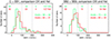 |
Fig. 6. v sin i distribution derived from O III (green) and He I (red) for single-lined stars (left) and for stars in SB2+SB3 systems (right). Only stars with v sin i measurements in both O III and He I are used. The histogram bin size is 20 km/s. The vertical dotted lines separate slow, medium, and fast rotators. The number of stars in the slow, medium, and fast bins and in total are given, as well as the modes of the distributions. |
To conclude, in the “transition region” around v sin i = 100 km/s the mixed use of O III and He I leads to a small bias. For comparing the number of slow and increased rotators between single and double-lined stars, the bias is about 11%. For each comparison in the sections below, we have carefully checked, if the differences between subsamples may be due to the (partial) use of non-metal lines and how strong this effect is. We found that the exclusive use of He I instead of O III does not alter the results and conclusions drawn below.
4.2. v sin i comparison with literature
A comparison with the literature allowed us to check the quality and reliability of our results.
We compared the v sin i results of our 166 C/SB1 stars with those of the IACOB & OWN surveys (285 C/SB1). We found a match of 135 stars with the latest catalog by Holgado et al. (2022), who have carefully derived v sin i from a combination of the FT method with GOF. Figure 7 illustrates the overall good agreement. Two notable differences are:
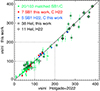 |
Fig. 7. Comparison of v sin i of C and SB1 stars from this work with those measured by Holgado et al. (2022). The values scatter around unity (solid diagonal line). Regarding the C/SB1 classification, the Holgado et al. sources with line profile variation (LPV) are matched with our Cs. Stars with different C/SB1 classifications are marked: we find more slow SB1s (red) and Holgado et al. find more fast SB1s (blue). |
(1) Among slow rotators (< 100 km/s) there is a group of six stars where we find larger v sin i than Holgado et al. Our v sin i value of these stars is based on He I instead of O III. A detailed check shows that these are mostly single stars (C) and equally balanced among dwarfs and giants. We do not expect that the use of He I instead of O III alters the results and conclusions below.
(2) We find 7 more slow SB1 and Holgado et al. find 5 more medium and fast SB1. This difference could be due to spectra observed at different orbital phases with better RV separation. An additional explanation could be, that our SB1 criterion uses the FWHM of the line profile (i.e. a flexible threshold), while Holgado et al. switched from a flexible to a fixed threshold, if v sin i < 180 km/s. Without going into details we emphasise that the results and conclusions drawn from our and Holgado et al.’s sample largely agree.
The stars classified as C by our spectra but as SB1 by Holgado et al. are listed as ‘C (SB1)’ in Table D.1. To use the most actual classification in the scientific analysis, for the rest of the paper we treat these stars as SB1s.
In the literature we found a match for 85 stars with listed v sin i values. The literature compilation is listed in Table D.2. The v sin i comparison is shown in Fig. 8, illustrating overall good agreement within 30%. A bias towards larger literature v sin i values may be explained as follows: Many literature v sin i values were estimated from the line FWHM (e.g. Penny 1996; Howarth et al. 1997), while we used the FT method; likewise our v sin i is largely based on O III 5592, while in the literature He I lines were used.
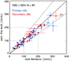 |
Fig. 8. Comparison of v sin i of disentangled SB2 and SB3 components from this work with collected values in the literature (Table D.2). The values scatter around unity (solid diagonal line), within ∼30% (dashed lines). The black arrows are upper limits. |
4.3. v sin i dependence on spectral type and luminosity class
The aim is to see whether spectral type or luminosity class have a significant effect on v sin i, and whether this may influence the v sin i dependence on SB type. Compared to single stars v sin i of binaries is on average increased (Sect. 4.4), so that trends with spectral type or luminosity class may be blurred. Therefore, we restrict the v sin i dependence on spectral type and luminosity class to the 130 Cs (presumably mostly single stars, but see Fig. 3 of de Mink et al. 2014). We consider v_peak and its standard deviation, calculated via the mode of the v sin i distributions.
We separate giants and dwarfs. Within each group, stars of spectral type earlier or equal O7.5 show a ∼10 km/s faster v_peak than later spectral types (v sin i-mass trend, Fig. 9). For instance, the highest blue histogram bar is shifted by one histogram bin (20 km/s) against the highest red histogram bar. So far, however, only tentative observational evidence for that trend between early- and late-type stars has been presented, partly because the v sin i distributions are broad and the samples were small. Examples are given by Conti & Ebbets (1977, their Fig. 6), and by Simón-Díaz & Herrero (2014, their Figs. 14 and 15). We see the v sin i-mass trend clearly in our data, but in view of the broad standard deviations the statistical significance is small. We mention three possible explanations:
-
(1)
An earlier (and more massive) dwarf has a larger radius R*, so that for a given angular velocity, ω, the earlier dwarf exhibits a larger v sin i; for giants, however, this explanation does not work because R* decreases from late to early giants.
-
(2)
If early-type stars have a stronger macroturbulence or wind component than late-type stars, then a bias, as explained in Appendix B, may lead to a larger v sin i in the earlier types.
-
(3)
Compared to late-type stars, early-type stars are, on average, a factor of ∼2 more massive and a factor of ∼5 more luminous. This makes it harder to detect a companion, either by dRV or by discerning the spectral lines of the companion. Therefore, the fraction of Cs with detection-escaped companions might be higher among early-type stars. Such Cs are then actually binaries and may have a larger v sin i (Sect. 4.4).
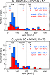 |
Fig. 9. Dependence of v sin i of single stars (C) on spectral type and luminosity class. Among giants and dwarfs, respectively, the early-type stars (blue) show a ∼10 km/s faster v_peak than the late-type stars (red). Likewise, the v_peak of giants is faster than that of dwarfs. |
The v sin i-mass trend may provide interesting clues to processes in O stars, but a detailed exploration is beyond the scope of this paper.
Similar to the v sin i-mass trend, Fig. 9 shows also a v sin i-LC trend: for a given spectral type range, the dwarfs show a slightly slower v sin i peak than giants and supergiants. This trend was previously seen with a stronger difference between dwarfs and giants (Conti & Ebbets 1977 and subsequent works). We note here that giants have a larger radius than dwarfs (a factor of 2-4 depending on the spectral type, Martins et al. 2005a). For the angular momentum (a fundamental quantity with conservation law) the angular velocity, ω, is relevant. Here we use alternatively the rotational period Prot = 2πR*/v, with stellar radius R* from Martins et al. 2005a. Figure 10 shows the distribution of Prot. In terms of period, on average, the giants and SGs rotate significantly (30–40%) slower than dwarfs. This result supports the consensus view that the rotation is braked during the stellar evolution.
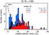 |
Fig. 10. Rotational period of single stars. Prot = 2πR*/v. The vertical dotted line at Prot = 5 d corresponds to v ≈ 100 km/s for an O7.5 V star. Dwarfs exhibit a clear short-period peak. The median period is given for the bulk of stars with long periods > 5 d. |
Another topic is the distribution of dwarfs in Fig. 10: above and below the 5 d line it appears split into two different components. We suggest that this bimodal appearance is real, but difficult to interpret. It is certainly of formal (mathematical) nature: when plotted versus Prot, the view onto slow rotators is zoomed, but all increased rotators (v sin i > 100 km/s) are “compressed” into a small range leading to the strong histogram peak below the 5 d line. Further details are beyond the scope of this paper.
Both v sin i-mass and v sin i-LC trends are also present when v sin i has been measured only with the O III 5592 line and not with He I lines; this shows that the usage of He I lines does not significantly biases the v sin i statistics of our samples. In addition, both trends are weak, suggesting that they have only little effect compared to other v sin i trends and statistical v sin i differences below.
4.4. v sin i dependence on SB type
So far the sample, for which we have determined v sin i, consists of 130 Cs, 36 SB1s, and 140 stars in 64 SB2 and 8 SB3 systems (72 primaries, 62 secondaries and 6 tertiaries). Figure 11 shows the v sin i dependence on SB-type:
-
(1)
For each SB-type, most stars are slow rotators with v sin i around 40–100 km/s.
-
(2)
Spectroscopic binaries (SB1/SB2/SB3) show a factor of 2 larger fraction at medium v sin i between 100 and 200 km/s, compared to single stars (C).
-
(3)
The singles stars show a larger fraction (15%) of fast rotators (v sin i > 200 km/s) than the binaries (SB1 5%, 10% SB2+SB3).
-
(4)
The separation of luminosity classes into dwarfs (IV+V), III and I+II shows that dwarfs dominate the binary population (dwarf fraction 121/176 = 69%), compared to the Cs (dwarf fraction 57/130 = 44%, giant/SG fraction 56%). The explanation for the larger giant/SG fraction in Cs is not straightforward: Fast evolution of one of the I/II components in a binary could make the system to appear as C or SB1 later. Also an observational bias against giants/SGs in SB2s could occur, since a giant/SG is more luminous making it harder to detect a less luminous companion.
-
(5)
The results and trends are already seen in the pure O III sample (Fig. 6) but they are more pronounced in the full sample. This is due to the larger sample size and the fact that typically medium and fast rotators are harder to measure in O III.
-
(6)
The v sin i distribution of the 27 B-type secondaries appears similar to that of the O stars in binaries; differences might be due to the low number statistics. The inclusion of B-type secondaries does not significantly alter the results.
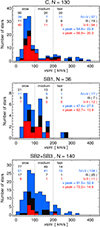 |
Fig. 11. v sin i distribution of the spectroscopic binary types. The 140 stars in SB2+SB3 systems are 72 primaries, 62 secondaries, and 6 tertiaries. v_peak gives the mode and standard deviation of the v sin i distributions for LC I+II (red) and IV+V (blue); LC III has too few data points. |
For the further analysis and discussion we use the full sample including the B-type companions.
5. Increased rotation rate in binaries
The rotation rate of binaries shows a clear excess at medium v sin i (100 km/s < v sin i < 200 km/s) compared to stars classified as C (Fig. 11). On the other hand, fast rotators (v sin i > 200 km/s) are more frequent in Cs than in binaries at all. Cs may be true single stars or intrinsic binaries which escaped detection due to small dRV arising from poorly inclined orbital axis, very wide orbits and very low mass ratio M2/M1. The aim is to understand the observed rotation difference between binaries and Cs, with the key question of what leads to the increased rotation in binaries.
Holgado et al. (2022) have reported a medium v sin i excess in SB1s and ascribed it to binary interaction during massive star evolution. Britavskiy et al. (2023) have investigated the post-interaction nature of fast rotators (v sin i > 200 km/s) and their rareness among binaries compared to Cs. Sana et al. (2012) have analysed the O star population (31 C, 7 SB1 and 33 SB2) of six nearby Galactic open stellar clusters. To conclude on the role of interactions on the binary evolution, they performed Monte Carlo simulations of interacting massive stars and compared them with the orbital period, eccentricity and mass ratio measured for the SBs. They briefly addressed spin-up of the secondary by donor-gainer mass transfer. However, they did not include measurements of v sin i.
Ramírez-Agudelo et al. (2015) have found in the VLT-Flames study of the 30 Doradus region of the LMC, that SB1 and SB2 rotate faster, if they have a large radial velocity difference (dRV > 200 km/s) which serves as a proxy for a short orbital period (Porb < 10 d) and a small separation of the components. Our O-star sample provides a large statistical v sin i study of SB2s in the Milky Way and we use measured orbital periods.
Of course, the detection of a spectroscopic binary is affected by the inclination of the orbital axis; likewise, v sin i of individual stars is affected by the inclination of the rotational axis. Thus, it is tempting to “unify” binaries and Cs via orientation, where at least part of the Cs are misaligned binaries. Statistically, however, inclination plays a minor role on v sin i (in the range of 10%) and fails to explain the rotation differences between the samples; more details are given in Appendix C.
Therefore, interaction between binary components has to be considered, in other words spin-up both by tidal synchronisation when the components approach (Zahn 1975, 1977; Tassoul & Tassoul 1997) and by mass exchange and merging (de Mink et al. 2013). The components in our sample are separated by less than 30 AU down to 0.1 AU (Fig. 12). For comparison, the distance between Neptun and the Sun is 30 AU. If the common assumption holds that O-type binaries are born with a component separation of at least several hundred AU (e.g. the massive proto-binary found by Zhang et al. 2019), then it is tempting that our data provide insight to the spin evolution during the approach of the components.
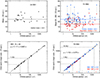 |
Fig. 12. Calibration mass and semi-major axis vs. orbital period. Left for SB1 and right for SB2. Top: Mass, the horizontal line marks the median mass. Bottom: Semi-major axis, the solid line marks a least-squares fit to the data (logarithmic, with the fit equation labelled). The vertical and horizontal lines are for guidance (dashed and dotted). Bottom right: Blue and red distinguish the mass ratio, the coloured numbers give the number of SB2s in the Porb bins separated by Porb = 10, 100, 1000. |
We here focus on how the rotation of primary P and secondary S changes from wide to close binaries6. The separation of the components is inferred from the orbital period, Porb. Because for most SB systems our spectra are sparsely monitored, the period information is collected from the literature (Tables D.1 and D.2). This yields subsamples with v sin i and Porb containing 24 out of 36 SB1s (67%) and 70 out of 72 SB2s (97%, including the 8 SB3s). The respective v sin i histograms (for SB1, P and S) of the subsamples look – apart from absolute numbers – similar to those of the original SB samples, suggesting that the subsamples provide robust statistical implications and conclusions.
5.1. Rotation difference between close and wide binaries
We divide the sample into close and wide binaries applying a threshold of Porb = 10 d which is justified further below; this threshold has also been applied by Ramírez-Agudelo et al. (2015) for O stars in the LMC. We converted Porb into semi-major axis, a, using the (re-written Keplerian) equation
 (2)
(2)
with Porb in days, mass M1 + M2 of the two components in M⊙ and a in R⊙. For M1 and M2 we used the “calibration mass”, which is the stellar mass from the (interpolated) tables in Martins et al. (2005b), corresponding to the spectral type and luminosity class of the SB components (listed in Tables D.1 and D.2). For SB1s we adopted M2 = 0.1 ⋅ M1. For one SB2, V 961 Cen, we used the mass from Doppler tomography (Penny et al. 2002) which is about a factor of 2 smaller than the calibration mass and leads here to more consistent results.
Figure 12 (top) shows stellar mass versus Porb. Across the entire Porb range, SB1 and SB2 have similar median primary mass M1 of about 25 M⊙. For SB2s the median secondary mass M2 is about 15 M⊙ (i.e. 2/3 of M1). The number of long period SB1s, and SB2s with M2/M1 < 0.5 declines at Porb ≳ 100 d. This is likely an observational bias against detection of wide binaries, but it does not affect the findings and conclusions on the wide binaries below (see Sect. 5.3).
Figure 12 (bottom) shows a versus Porb. The least-squares fit to the (logarithmic) data agrees well with  . The moderate scatter around the fit is due to deviations of the calibration mass from the real one. For our sample, Porb = 10 d corresponds to a ≈ 60 R⊙, and a = 1 AU to Porb ≈ 70 d.
Figure 13 shows v sin i versus Porb of the SB systems. It reveals:
-
(1)
For SB1s, all medium rotators lie at Porb < 30 d, while slow rotators distribute evenly across the entire logarithmic period scale (top left panel).
-
(2)
For SB2s, the components distribute across the entire parameter space (top right panel). There are clear trends – like for SB1s – when P and S are plotted separately (two bottom panels): the medium rotators concentrate at short Porb < 10 d, and most of the slow rotators are at long Porb > 10 d.
-
(3)
Among SB2s, there are few fast rotators. Notably, fast primaries are preferrably located among close SB2s, and fast secondaries among wide SB2s. (Among SB1s, the period of the only one fast rotator, HD 041997, is not known.)
-
(4)
Giants distribute across the entire period range. The giant incidence is larger in SB1s than SB2s and among SB2s it is larger among primaries and among close SB2s. Among the wide SB2 primaries, all but one are slow rotators.
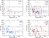 |
Fig. 13. v sin i vs. orbital period. Top: For SB1 (left) and SB2 (right), each primary–secondary pair is connected with a vertical dotted line. Bottom: SB2 primaries and secondaries plotted separately; for the secondaries the black encircled symbols mark B-type companions. |
The trends are corroborated by the v sin i histograms in Fig. 14. Top row: Both close primaries and secondaries reveal a strong excess of medium rotators. Bottom row: The v sin i distribution of wide primaries is dominated by slow rotators and appears similar to that of Cs (cf. Fig. 11). However, wide secondaries are different exhibiting a strong fast tail. Removing B-type secondaries yields similar histograms. In addition, separating close and wide binaries by Porb = 20 d (instead of 10 d) yields similar histograms. To summarise, close binaries exhibit a pronounced spin-up further analysed in Sect. 5.2. On the other hand, wide primaries, on average, appear similar to Cs dominated by slow rotators, and wide secondaries appear nearly bi-modal with a dominant slow rotator peak and a strong spin-up peak; this is discussed in Sect. 5.3.
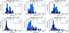 |
Fig. 14. Histograms of v sin i for close and wide SB2s separated by Porb = 10 d, from left to right for primaries, secondaries, and the entire samples. Top row: Close SB2s. Bottom row: Wide SB2s. |
5.2. Synchronisation and mass transfer in close binaries
The two mechanisms discussed are:
(1) Spin-orbit synchronisation aligns the rotational and orbital axes and equalises the periods ( ). It may increase but also brake the stellar rotation (e.g. Zahn 1977). It predicts an increased equatorial stellar rotation (v > 100 km/s), if Porb ≲ 10 d. On the other hand, at Porb = 10 d spin-orbit synchronisation will brake a fast rotating O9 I star with v = 300 km/s (Prot = 4 d).
(2) Mass transfer (MT) from an expanded mass donor (typically the primary) to a mass accretor (the gainer, typically the secondary) increases the spin of the gainer, while that of the donor may be reduced. Since the mass flow is in the orbital plane, MT may align the rotational and orbital axes (and aligned axes have been generally assumed in simulations, e.g. Wellstein 2001; de Mink et al. 2013).
If both mechanisms synchronisation and mass transfer are at work, we expect (1) the primary period to equal that of the orbit (neglecting spin down of the mass donor) and (2) the secondary period to be equal or shorter than that of the orbit.
We will not examine each SB system individually but perform a statistical analysis. Our chain of reasoning begins with assuming – as a guide line – that the binaries are synchronised, testing how far the data are consistent with synchronisation using the simple criterion that the periods should be equal. Then, we look how far the deviations between data and the ideal synchronisation picture are consistent with the mass transfer scenario. We will use suited examples for illustration.
To check for synchronisation, we will compare Porb and Prot. Porb is precisely available from radial velocity curves (with an error smaller than 1%). However, direct measurements of Prot are not available. We derived Prot from the measured v sin i and calculated the auxiliary quantity
 (3)
(3)
which still depends on the inclination. The inclination will be rectified below (Sect. 5.2.2). The error of v sin i lies between 10% and 30%. The uncertainty of Prot is likely dominated by the choice of R*.
For R* we take the “calibration radius” (i.e. the stellar radius) from the logarithmically interpolated tables for spectral type and luminosity class in Martins et al. (2005b) (see Tables D.1 and D.2). For 19 SB2s in our sample, the actual stellar radius was measured by various authors, for example with eclipses or inferred from luminosity considerations, if the distance was known. We denote it the literature radius Rlit. It is listed together with references in Table D.2. Figure 15 shows that Rlit is on average ∼10% smaller than R*; this has already been noted for some O binaries by Rauw et al. (2001a). The standard deviation of Rlit/R* indicates that the uncertainty of R* is at least 20%. Nevertheless, we here use the calibration radius and discuss the outcome. An exception is V 961 Cen where we used the literature radius (Penny et al. 2002), which is a factor 2–3 smaller than the calibration radius and here yields more consistent results.
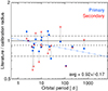 |
Fig. 15. Ratio of literature to calibration radius Rlit/R* of the stars vs. orbital period for the 19 SB2s where a literature radius is available (Table D.2). For each SB2 the vertical dotted line connects the primary and secondary. Unity is marked by the horizontal solid line, and the average and its standard deviation by the horizontal long-dashed and dash-dotted lines, respectively. The blue three-dot-dashed line is an ordinary least-squares fit (log Y vs. log X) of the primary data. |
For comparison, we have calculated the effective Roche radius Rroche of all stars using the formula by Eggleton (1983). If Roche lobe overflow (RLOF) is frequent in the primaries, then one would expect for them that Rlit ∼ Rroche which may reach up to 2 R*. Notably, this is not seen in Fig. 15. Furthermore, if RLOF is frequent in close but not in wide binaries, then one may expect a trend of increasing Rlit/R* with decreasing orbital period. Therefore, in Fig. 15 we have plotted Rlit/R* versus Porb. However, such a trend is only marginally visible (blue 3-dot-dashed line) and appears not yet of statistical significance in this small sample of 19 SB2. A precise measurement of the actual stellar radius is challenging. In view of the uncertainties, we think that the results on Rlit/R* obtained so far do not argue striktly against RLOF in close binaries, rather they appear consistent with partial Roche lobe filling of the primaries.
5.2.1. Close SB1s
We begin with how far synchronisation may lead to a spin-up of v sin i from slow to medium rotators (i.e. crossing the threshold of 100 km/s). We consider the close SB1s in Fig. 13 (top left) and Fig. 16 (top left):
-
(1)
four giants with medium v sin i (blue dots with black cross)
-
(2)
two dwarfs with medium v sin i (blue dots without black cross)
-
(3)
three dwarfs with slow v sin i (red dots without black cross).
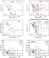 |
Fig. 16. Dependence of rotational properties on the orbital period. Top: Rotational period vs. orbital period for SB1s (left) and SB2s (right). The y-axis of Fig. 16 is inverted in order to preserve that faster (slower) rotating stars are plotted up (down). The vertical long-dashed line separates close and wide binaries. The solid diagonal line labelled ‘sync’ marks equal periods, as required for synchonised rotation, whereby an inclination i = 30° of the rotational axis shifts the data points from this line by a factor of 1/sin(30°) = 2 to the dotted inclination line labelled ‘i = 30’. The two SB2s below the dotted inclination line indeed have known iorb < 20° (HD 048099 and HD 167771). For SB2s, the components are connected with a vertical dotted line; for most wide binaries at Porb > 10 d, Prot differs strongly between the components but the difference reduces and disappears for close binaries. Middle left: Ratio of Prot of the binary components vs. Porb; the horizontal lines mark the median in each Porb range. Middle right: Prot vs. Porb for those 53 SB2s with known inclination of the orbital axis iorb; Prot is corrected for inclination assuming parallel orbital and rotational axes. The solid and dotted diagonal lines mark the synchronisation range with a width of 30% and a factor of 2, respectively. The green triangle marks the range above the sync line discussed in the text. Bottom left: v sin i vs. Porb for the 53 SB2s with known iorb. Bottom right: veq vs. Porb after correction for the inclination. |
Despite having different v sin i, all of these stars (except one discussed below) lie in a narrow range between the sync line defined by Prot/sin(i) = Porb (solid diagonal line) and the dotted line labelled i = 30 (Fig. 16). Inclination, if present, shifts the stars down by a factor f = 1/sin(i), e.g. f = 2 for i = 30°. The inclination of the SB1s is not known and cannot be corrected here. Nevertheless, it appears consistent that SB1s which are close to or below the sync line are synchronised. Then it is tempting to speculate that the SB1s with medium v sin i (blue dots) originally (i.e. in the past) were slow rotators and received a spin-up during the approach and synchronisation of the components. We will discuss this possibility further for those SB2s where inclination is corrected.
The examples illustrate also that the analysis of v sin i alone is not an ideal spin-orbit indicator, because the stellar radius plays a crucial role on Prot. The radius increases from late to early dwarfs by about a factor of 2. Giants have a factor of 2-4 larger radius than dwarfs. Even slow rotating SB1s may be synchronised, if their radius is small enough. Synchronisation may begin already at Porb = 30 d but there the stars would be slow rotators. The threshold of v sin i = 100 km/s corresponds to Prot/sin(i) between 5 and 10 d, depending on the stellar radius; this can be seen from the vertical distribution of the blue and red symbols in Fig. 16 top left.
One close SB1 lies a factor of 2 above the sync line (HD 053975 v sin i ≈ 180 km/s, Fig. 16 top left). Obviously it rotates too fast for the pure synchronisation scenario. We address two possibilities which could bring HD 053975 into a consistent picture:
-
(1)
Fast rotation deformes a spherical star to a lenticular star with increased equatorial radius Req ∼ 1.5 ⋅ Rpolar. However, this requires between 40–50% and up to 90% of the critical rotation (i.e. veq between 250 and 500 km/s) (Abdul-Masih 2023; Maeder & Meynet 2000; Maeder 2009). For HD 053975 the inclination of the rotation axis is not known; if irot = 30° then veq ≈ 360 km/s, in the range required for deformation but then HD 053975 will lie a factor of 4 above the sync line, exceeding a possible down-shift by the factor 1.5 due to deformation. Thus, an additional mechanism is required.
-
(2)
In case of (partial) Roche-lobe filling the actual radius is larger than the calibration radius used to convert v sin i to
 . This may shift HD 053975 towards the sync line.
 -
(3)
On the other hand, if the R* (used for the plot) is indeed the actual stellar radius, then HD 053975 is not (yet) spin-orbit synchronised. Then it has already a high spin, somehow obtained in the past. One may speculate that the ongoing tidal forces may spin-down HD 053975. This and/or a potential further approach of the components may finally move HD 053975 to the synchronisation line.
To conclude, the close SB1s populate a range of Prot/sin(i) vs. Porb which is consistent with spin-orbit synchronisation. In some cases an expanded stellar radius, e.g. by (partial) Roche-lobe filling, of the SB1 primary may be implied.
5.2.2. Close SB2s
Figure 16 (top right) displays Prot/sin(i) vs. Porb. To understand what happens in the close SB2s, we first compare with the wide SB2s. Wide binaries with Porb > 10 d exhibit a large difference (on the logarithmic scale) between  and
and  , marked by the vertical dotted lines connecting the SB2 components. This difference provides evidence that wide SB2s are not synchronised, because the components have different periods or inclinations. However, for close binaries the rotational periods of the components converge.
The convergence of the rotational periods is visualised by the ratio  of the rotational period, either
  or
or  , whereof the value < 1 is used (Fig. 16, middle left). The blue dots mark SB2s, where (in terms of angular velocity) the primary spins faster than the secondary, and vice versa for the red crosses. The advantage of the ratio is that the effect of inclination cancels, if the rotation axes are parallel as assumed to be the case for synchronisation; therefore we have omitted the term sin(i). The median
  is about 0.5 for wide binaries (in two bins separated by Porb = 100 d) and increases steeply to 0.8 for close binaries. Given the uncertainty of about 20% in the stellar radius (Fig. 15) and allowing for a small inclination difference, it is tempting to accept
  as consistent with unity. This argues in favour of synchronised rotation in close SB2s. The sudden rise for
  at Porb ≲ 10 d also supports the choice Porb = 10 d to separate between close and wide binaries. We note that the ratio is suited for a consistency check (i.e. whether synchronisation could be present), but it requires that the stellar radius (used to convert v sin i to rotational period) is precise enough.
Therefore, we further examine the effect of inclination, sin(i), visible in Fig. 16 (top right). Like for the SB1s, inclination shifts the close SB2s below the “sync” line. Synchronised rotational and orbital axes are assumed to be parallel (iorb ≈ irot), so that knowledge of iorb allows us to correct for irot. For 53 SB2s in our sample the inclination of the orbital axis, iorb, is known (Table D.2). iorb has been inferred from Msin(i)3 measurements and the calibration mass (Martins et al. 2005b). For these SB2s, we corrected Prot via multiplication with sin(i). We note that wide binaries may not be synchronised, and the inclination correction for them should be considered with caution. The result is shown in Fig. 16, middle right. After correction, about 40 of the 62 close binaries lie inside the sync range ±30% around the “sync” line. Given the uncertainty of v sin i, stellar radius and inclination, it appears reasonable to adopt an uncertainty of 30% for Prot. Strikingly, there are no stars in the region below the sync range. Such stars would rotate too slowly for being synchronised. For the 53 SB2s with known iorb, Fig. 16 bottom right and left show v sin i as observed and the equatorial velocity veq after correcting for the inclination. Indeed, the close SB2s lack slow rotators; almost all are increased rotators with veq > 100 km/s (see also the histograms in Fig. C.1). On the other hand, there exist many slow rotators among wide SB2s. It is plausible that the wide SB2s evolve to become close SB2s. This strongly suggests that any originally slow rotating components increased their rotation rate during the approach and synchronisation.
About 20 of the 62 close SB2 components (∼30%) lie above the sync range in a region marked by the green triangle (Fig. 16 middle right); 7 components lie even above the upper dotted sync line. These stars appear to rotate too fast to match synchronisation. This suggests that additional mechanisms play a crucial role. To shift the stars in the green triangle down to the sync range, we have to increase Prot, hence enlarge the used calibration radius to the synchronised radius Rsync. To obtain a consistent picture, this implies:
-
(1)
For fast rotators: the equatorial radius is increased, but this is limited to a factor of ∼1.5 (Abdul-Masih 2023). However, most stars in the green triangle are not fast rotators.
-
(2)
For the primaries: the radius is increased by (partial) Roche-lobe filling or Roche-lobe overflow (RLOF). This strongly supports the presence of mass transfer in these SB2s.
-
(3)
For the secondaries: spin-up by mass transfer likely acts against spin-orbit synchronisation. Therefore, it is consistent that secondaries are seen also above the sync range. There is no need to shift the secondaries towards the sync line. In addition, the duration of the spin-up phase is short (cf. Fig. 2 in de Mink et al. 2013). Therefore, not all secondaries must be seen currently in a spin-up phase. As a consequence, secondaries may reside both close to and above the sync line.
We illustrate the increase of the radius with few examples, where the primary lies above the sync line. They are labelled in Fig. 16, middle right:
-
(1)
HD 152218 at Porb = 5.6 d,
 d,
d,  d, with i ∼ 71°. This is a binary with clear evidence for wind-wind interaction, hence mass located between the components supporting that MT is indeed present (Sana et al. 2008a). To shift the primary to the sync line requires an increase of the radius from R* = 10 R⊙ by a factor of 5.6/3.3 = 1.7, yielding Rsync = 17 R⊙, lying well inside the Roche-Radius Rroche = 22.8 R⊙. Both components are medium rotators with inclination corrected equatorial rotational velocities v ∼ 150 km/s.
 -
(2)
HD 149404 consists of two super-giants with Roche lobe overflow episodes during the past (O7.5 I, v sin i = 88 km/s, ON9.7 I, v sin i = 71 km/s), Porb = 9.8 d,
 d,
d,  d, with i = 24° (Rauw et al. 2001b; Raucq et al. 2016). Both components are medium-fast rotators with inclination corrected equatorial rotational velocities v = 216 km/s and 175 km/s. To shift the primary to the sync line requires an increase of the radius by a factor of 9.8/4.8 = 2.04, yielding Rsync = 42 R⊙, still consistent with Rroche = 40 R⊙.
 -
(3)
HD 165246 has a fast primary (O8 V, v sin i = 221 km/s) and a slow-medium secondary (B0: V, v sin i = 100 km/s), with i = 83°, Porb = 4.6 d,
 d,
d,  d (Mahy et al. 2022). To shift the primary to the sync line requires an increase of the radius by a factor of 4.6/1.9 = 2.4, yielding Rsync = 20.3 R⊙, slightly below the Rroche = 22.7 R⊙.
 -
(4)
HD 163892 has a medium-fast primary (O9.5 IV, v sin i = 183 km/s) and a very slow secondary (B0: V, v sin i = 39 km/s), with i = 70°, Porb = 7.8 d,
 d,
d,  d (Mahy et al. 2022). To shift the primary to the sync line requires an increase of the radius by a factor of 7.8/2.5 = 3.1, yielding Rsync = 30 R⊙, similar to Rroche = 29.5 R⊙.
In the two last examples, the secondary has a moderate inclination corrected equatorial rotational velocity v (HD 165246: v ∼ 102 km/s, HD 163892: v ∼ 41 km/s). In terms of angular velocity, however, the spin of the secondary is a factor (2.7, 1.5) faster than that of the orbit. If the radius of the secondary is indeed correct (and thus  ), this implies a spin-up by mass transfer even in slow rotating secondaries.
For the stars in the green triangle we have seen that the actual radius (in particular of the primary) may be larger than the calibration radius used. (If a star in the green triangle were correctly positioned, then it had already spun-up by any mechanism and we discuss this possibility in Sect. 5.3.) In principle, also the remaining stars close to the sync range may have an increased actual radius. If true, this may shift them below the sync range. Then they rotate too slow for being synchronised. The timescale to reach synchronisation is between 0.5 and 5 Myr depending (besides other parameters) on the separation a/R* (Fig. 3 of Zahn 1977). Thus the stars could still be on the way to become synchronised.
The distinction between sync range and green triangle arises during our chain of reasoning. Therefore, we consider it unlikely that the close SB2s split into two physically distinct populations, one with calibration radius perfectly matching the sync line and one needing an expanded radius. This leads to the conclusion, that the spin is not only controlled by synchronisation. Rather, binary interaction involving Roche-lobe filling and mass transfer (MT) plays a strong and presumably dominant role for spinning-up.
For HD 093161 A at Porb = 8.6 d the O7.5 V primary appears on the sync line, but the O9 V secondary lies below the sync range suggesting that it is not yet synchronised. A plausible explanation is that the rotational axis of the secondary is not aligned with the orbit axis. The orbit inclination is 84°. The system is a well isolated SB2 (DT 1). Both components are slow rotators with v sin i = 48 km/s and 31 km/s, robustly measured in O III 5592.
Finally, we pay attention to HD 047129 (Plaskett’s star), a well studied binary considered to be a prototype of spin-up by mass transfer. With Porb = 14.4 d (a = 96 R⊙), the system lies near the border between close and wide binaries. It consists of a slow rotating primary (O8 I, v sin i = 80 km/s) and a fast secondary (O8.5 fp, v sin i = 236 km/s), with i = 71°,  d,
d,  d (Bagnuolo et al. 1992; Linder et al. 2008). The primary is a super-giant with a calibration radius of about 40–50% of the Roche radius. The primary lies perfectly in the sync range, while the secondary has spun-up by a factor of ∼5 compared to Porb.
For slow rotating stars synchronisation is possible at 10 < Porb/d < 30, but the range Porb < 10 d is relevant for a synchronisation-induced spin-up (v sin i ≳ 100 km/s). Therefore we have chosen Porb = 10 d as threshold between close and wide binaries Furthermore, if a star lies above the sync range, then in principle, synchronisation may brake its rotation.
To conclude, close SB2s contain slow, medium and a very few fast rotators. Conversion of v sin i to Prot and correcting for inclination, yields the formal result that 70% of the stars lie in an ideal range for spin-orbit synchronisation. About 30% of the stars lies above that sync range, implying that the primaries have an expanded radius (e.g. due to RLOF), consistent with the presence of mass transfer which in turn spins-up the secondaries. The separation of the stars in two distinct groups is likely of formal nature. From our statistical point of view, the spin-up of the close SB2s can fully be explained by a combination of ongoing synchronisation and mass transfer. The scarcity of fast rotators remains puzzling.
5.3. Increased rotators in wide binaries
The sample contains 15/24 (62%) wide SB1s and 39/70 (56%) wide SB2s. Compared to the SB1s, the larger number of SB2s allows for better statistics and the comparison of primary and secondary provides further insight. Therefore, we here restrict the discussion on the SB2s and, if suited, mention SB1s in comparison with SB2 primaries.
The rotation rate of wide SB2s (primaries and secondaries together) shows a pronounced peak at v sin i ∼ 50 − 80 km/s (Fig. 14, bottom right). At first glance, it is reminiscent to that of Cs (Fig. 9, top). About 35% (27/78) of the wide SB2 components are increased rotators (Fig. 14). What increased the rotation in the medium and fast wide binaries? Or were they born with increased rotation? The period difference between primary and secondary rejects an increase by spin-orbit synchronisation (Fig. 13). We first discuss how far the wide binaries could be spun-up by mass transfer (Sect. 5.3.1). This turns out to be not satisfying. Therefore, we discuss alternative spin-up mechanisms in Sect. 5.3.3.
5.3.1. Spin-up by mass transfer
A testable prediction of MT-based spin-up in wide binaries is that the gainer rotates faster than the donor. We first assume that the more massive component (the primary) is the donor. We count the number of increased rotators among the secondaries: 17/39 (∼44%) from Fig. 13 and Fig. 14 (bottom middle panel). All of them rotate faster than the primary; we call these binaries “seco-fast” (they are marked by large red symbols in Fig. 17). The mass ratios M2/M1 of the seco-fast binaries distribute between 0.27 and 1. At first glance, this altogether appears consistent with expectations for MT-based spin-up.
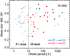 |
Fig. 17. Mass ratio vs. orbital period. Blue and red indicate whether the primary or secondary is the faster component (measured by v sin i). Among wide binaries, the large symbols mark those pairs where at least one component is a medium or fast rotator (6 blue and 17 red pairs; see Sect. 5.3.1). |
On the other hand, 10/39 (∼26%) of the wide primaries are increased rotators (Fig. 14). While 4 of these 10 have a secondary which rotates faster (and are plotted with a large red symbol in Fig. 17), 6 of these 10 wide primaries rotate even faster than the secondary (large blue symbols in Fig. 17); we call them “prim-fast”. If they are donors in the MT-scenario, one may wonder how they increased v sin i to > 100 km/s. At first glance, they appear to contradict the expectation of MT-based spin-up, where the gainer should rotate faster than the donor. Seeking to solve this puzzle, we find: The mass ratios M2/M1 of these 6 prim-fast binaries are closer to 1 compared to that of the seco-fast above. The similar mass ratio makes the distinction between donor and gainer uncertain. In the remaining 16 (= 39–17–6) wide binaries both primary and secondary are slow rotators. So far, the data statistics appears consistent with expectations for MT-based spin-up in wide binaries.
However, MT becomes inefficient for wide binaries with separation a ≳ 100 R⊙, corresponding to Porb ∼ 20 d and RRoche ∼ 50 R⊙. In addition, a significant spin-up of the secondary by capture of wind mass lossed by the primary can be excluded:
-
(1)
MT in binary stars occurs when (a) the star expands to fill its Roche-lobe or (b) the orbit, and thus Roche-lobe, shrinks until R* < RRL. RLOF is grouped into three cases: (A) MT while donor is on the MS, (B) donor is in the Red Giant phase, (C) Super-Giant phase. (For details we refer to de Mink et al. 2013.) The calibration radius R* of O- and early B-stars lies between 7 and 15 R⊙ (II-V), and reaches 25 R⊙ for luminosity class I (Martins et al. 2005b). While RLOF provides an efficient MT-based spin-up for close binaries, MT by RLOF becomes inefficient beyond a ∼ 100 R⊙.
-
(2)
Next we consider a possible mass and momentum transferred by a stellar wind. To increase the stellar spin by a factor of 2–5 (e.g. from v sin i = 60 km/s to 120 or 300 km/s, respectively), in an ideal acretion disk scenario a total accretion Macc of a few percent of the star’s mass M is needed (Packet 1981). We adopt the optimistic case Macc/M = 1%, hence for a 20 M⊙ star a required Macc ∼ 0.2 M⊙. The typical mass loss carried by a wind lies at 10−6–10−8 M⊙/yr (Howarth & Prinja 1989; Martins et al. 2005a; Vink 2022). For an isotropic wind, only a fraction of the wind mass ejected by the primary is captured by the secondary. For simplicity, this fraction is estimated by the solid angle Ω = (2πRcap2)/(4πa2). For a = 100 R⊙, adopting Rcap ≈ 2R* and R* = 10 R⊙ (an O5 V or O8 IV secondary), we obtain Ω ≈ 0.02. Adopting the optimistic case of a strong primary wind of 10−6 M⊙/yr, the required Macc is reached after 107 yr, exceeding the star’s life time.
Roche-lobe filling can be measured, for example by modelling eclipsing light curves for close binaries but hardly for wide binaries. To observationally establish the presence of a mass flow located between the binary components, one possibility is via the Struve-Sahade (S-S) effect: the apparent strengthening of a star’s spectrum as it approaches and weakening as it recedes (Struve 1937; Sahade 1959). Such investigations are challenging (e.g. Linder et al. 2007) and beyond the scope of this work.
Depending on the stellar mass and radius (luminosity class) MT-based spin-up is possible up to P ≲ 30 d, and some examples are:
-
HD 047129, an O8 I primary and an O8.5 fp secondary, Porb = 14.4 d, with a pronounced S-S effect (Linder et al. 2008).
-
HD 093403, O5.5 I + O7 V, Porb = 15.1 d (Rauw et al. 2002)
We note that both examples are formally wide binaries but near to the border to close binaries (Fig. 16, middle right). On the other hand, there exist examples against MT-based spin-up for wide binaries:
-
HD 093343 is comprised of two O7.5 Vz stars in a wide and eccentric orbit (Porb = 50 d, e = 0.4, Putkuri et al. 2018).
-
HD 096264, an O9.2 IV primary and a B0 V(n) secondary (Porb = 124 d, e = 0.2 Putkuri et al. 2021).
-
HD 054662, an O6.5 V(n)z and O7.5 Vz, notably the primary is a fast rotator while the secondary has slow v sin i ∼ 40 km/s (Porb = 2113 d, Barbá et al. 2020).
To explain the increased rotation in the three counter-examples, the authors argued:
(1) The wide separation in combination with the young age (∼2.5 to 4.5 Myr, implying small radii) excludes spin-up by RLOF. This conclusion is supported by our estimates of the low MT efficiency above. Spin-up by tidal interaction (spin-orbit synchronisation mechanisms) can also be excluded.
(2) The non-synchronous rotation of the components and the increased rotation of one component is likely a – not further specified – consequence of the stellar formation process. We note that this may lead to a puzzling picture as it implies that the fast spinning component has not suffered from rotational braking since birth, while the slow rotation of the coeval component requires a braking (or an unfavourable inclination of the rotational axis). Therefore, we consider possible scenarios in Sects. 5.3.2 and 5.3.3.
5.3.2. Initial velocity and rotational braking
After the birth of a single star, its initial rotational velocity vini decreases, and the braking rate depends on the combination of angular momentum losses due to stellar winds and the internal angular momentum transport from the core to the envelope. One may expect that this common view for single stars applies also to wide binaries, at least to those which are not affected by tides and mass transfer events.
Braking depends not only on the wind but also on internal momentum redistribution. The complex details require sophisticated modelling (Maeder & Meynet 2000; Langer 2012; Ekström et al. 2020). The rotational behaviour during stellar evolution is studied by theoretical models which are calibrated against observations.
Holgado et al. (2022) performed a thorough investigation using 255 single O stars with well-measured rotational velocity and well-determined position in the spectroscopic Hertzsprung–Rusell diagram (sHRD). They compared the empirical results to the predictions – regarding current and initial rotational velocities – of two sets of stellar evolutionary models (Ekström et al. 2012; Brott et al. 2011), that have been commonly used by the massive star community in the last decade. To summarise their results, both model sets do not provide a satisfying match to the data. In particular for numerous young slowly rotating stars (veq < 75 km/s) the models overpredict veq. Holgado et al. (2022) concluded that the models need a slower vini < 0.2 vcrit, compared to 0.4 vcrit typically adopted, or a stronger braking in the first 2–4 Myr after birth7. Therefore, the current models do not yet allow us to exclude (or imply) a substantial braking in the first 2–4 Myr after birth.
What can we learn from our wide SB2s about vini and rotational braking? A striking feature of our wide SB2s is the high fraction (∼70%) of non-synchronous rotation and, in addition, a strong “rotational asymmetry”: For most wide binaries the secondary rotates faster than the primary (Fig. 18). This feature holds for the set of 39 wide binaries and for the subset of 23 binaries where at least one of the components is an increased rotator (i.e. slow+slow pairs are excluded). The exclusion of the slow+slow pairs reduces potential noise in the distribution of the period ratios. Likewise, the trend holds for splitting the sample into 24 medium wide (10 d < Porb< 100 d, blue) and 15 very wide binaries (Porb> 100 d, red). Despite the small number statistics, incompleteness and potential biases of the sample, there is little doubt on the rotational asymmetry.
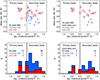 |
Fig. 18. Rotational asymmetry between primaries and secondaries, for all wide binaries (left column), and for a subset where at least one component is an increased rotator (right column). Medium wide and very wide binaries are coloured in blue and red, respectively. Top: Ratio of the rotation periods P/S vs. mass ratio; the size of the circles indicates the orbital period, i.e. component separation, on a logarithmic scale. Bottom: Histograms. |
A statistical analysis of non-synchronous wide SB2s may distinguish between two potential scenarios:
-
(1)
At birth or shortly after birth (∼2 Myr), both components are fast rotators and the currently observed slow component is braked or misaligned.
-
(2)
At birth or shortly after birth, both components are already slow rotators and the currently observed fast component had received a spin-up by any other mechanism.
We outline a tentative test to distinguish between the scenarios. The strategy is to consider scenario 1 for a subsample of non-synchronous SB2s with suited plausible assumptions so that only orientation differences between slow and fast component are left over to explain any difference of v sin i. Then we estimate the joint probability, Pjoint, of finding that many non-synchronous SB2s with a misaligned component as observed. We call these systems “misaligned”. At the end, a low Pjoint may argue against or in favour of scenario 1.
In detail, we assume (1) for each SB2 that the components A and B are coeval without tidal and mass transfer events, and (2) that A and B have not yet suffered from significant rotational braking, so that any increased rotation must be from birth. (A can be either the primary or the secondary, respectively.) Furthermore, if A and B are coeval and of sufficiently similar mass, any initial braking in the first ∼2 Myr should affect both components equally strong, thus we assume that both components have the same veq. (Indeed, the last assumption is supportd by the fact that the samples contain also pairs where both components have similar v sin i; mostly these are slow rotators.) With this set of plausible assumptions, we will consider the spin difference between A and B. Since other mechanism are excluded by construction of the test, the spin difference can only be due to the inclination difference of the rotational axes  and
and  .
.
In ∼70% of the wide SB2s, B spins a factor of > 2 slower than A. The factor 2 implies, for instance, if  , then
  , or if
  , then
  . To keep the experiment manageable, we define a common threshold for the inclination difference and
  . Conservatively adopting
  , yields
  . Then the probability of finding a single misaligned axis is i = 30° and P < 0.134 (adopting randomly oriented rotation axes; see Appendix C).
We determined the joint probability Pjoint of finding N or more misaligned systems among Nsample systems by calculating ten million experiments using a random number generator. Table 1 lists the Pjoint results for three samples (of Nsample = 39, 24, 15 SB2s) and N = 5, 10, 15. Two direct conclusions can be drawn:
-
(1)
To find just few (e.g. N = 5) misaligned systems, is relatively easy with Pjoint up to 0.61. However, the whole population of misaligned systems contains up to ∼70% of the samples. Conservatively adopting 50%, we have to use N ∼ 0.5 Nsample. Then Pjoint is very small (below 0.0001) rejecting scenario 1.
-
(2)
This leads us to favour scenario 2. It suggests a further generalisation to single O stars: without other interaction events, already shortly after birth (∼2 Myr) any O stars have become slow rotators, quasi as a “ground state of stellar rotation”. Then any increased rotation is likely not due to birth but requires other spin-up mechanisms.
The outcome of this test appears to consistently expand the conclusions of Holgado et al. (2022) above. A thorough implementation of this test needs a completeness and bias analysis of the wide SB2 sample, including a careful selection of those non-synchronous SB2 which certainly fulfil the assumptions, and a refinement of the assumptions. This is beyond the scope of our paper.
5.3.3. Spin-up mechanisms for wide binaries
Here, we consider possible spin-up mechanisms for wide SB2s. Each scenario should fulfil the following criteria:
-
(1)
It should be able to reach spin-up by factors of 2–5 (e.g. increasing v sin i from 60 to 120 or 300 km/s).
-
(2)
It should allow for “no spin-up”; in 16 (∼40%) of the 39 wide SB2 systems both components are slow rotators, whereby inclination is unlikely the main cause.
-
(3)
It should be consistent with the rotational asymmetry between primaries and secondaries (Fig. 18).
-
(4)
The timescale should be short (≲5 Myr) because of the short life time of massive stars.
Here, we discuss four possible scenarios to explain the increased rotators in wide SB2 systems:
-
(1)
We begin with revisiting the case that the binary stars are born with different spins (Fig. 19). Cause for the unequal rotation could be different cloud (or disk) fragmentation situations. Thus, two massive stars are possible that each bring their spin from birth. For simulations of the formation of binaries from accretion disks, we refer to Krumholz et al. (2009) and Oliva & Kuiper (2020), and for observations of large accretion disks and their fragmentation to Chini et al. (2004) and Ahmadi et al. (2023). Figure 19 intentionally shows the increased rotator being formed not from one single cloud fragment but from the merging of several (three) cloud fragments. This would easily explain the rotational asymmetry. However, it appears more likely that each cloud fragment forms its own star, and we come back to this further below. The O stars in our sample have already reached or evolved beyond the zero age main sequence (ZAMS). Then rotational braking could have taken effect, as discussed in Sect. 5.3.2. If the enlarged spin is from birth, the two questions that remain are identifying the mechanism that maintained the spin difference of the binary components so large and the reason why mostly the secondary spins faster than the primary.
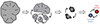 |
Fig. 19. Stars are born with different spins. Before the main sequence phase, fragmented cloud cores merged and the resulting stars feature slow (red) and increased (blue) spin. |
Next we assume that the stars have evolved beyond the ZAMS, have become slow rotators, which then spin-up by one of the following mechanisms:
-
(2)
Hidden SB1 mechanism: The wide SB2 system is actually a hierarchical (i.e. stable) triple system (Fig. 20). The increased rotator (primary or secondary) of the SB2 system is itself a close SB1 with a hidden (lower mass) component (tertiary C). Our sample contains two potential examples: (a) HD 152246 is a hierarchical triple system, consisting of a wide (
 d) SB2 with a hidden tertiary which is bound to the secondary B in a close circular orbit with a short period of
  d (Nasseri et al. 2014). This makes the secondary actually an SB1 with 18.4 and 4.4 M⊙ (the components are named Ba and Bb in Nasseri et al.). The short period suggests that the SB1 subsystem is synchronised, like the O-dwarfs plotted in red in the top left panel of Fig. 13.
  and radius of component B (spectral type O9 V) yield
  km/s, consistent with the observed v sin i (B) = 52.7 km/s. This argues for synchronisation of this SB1 subsystem, if
  (we recall that
  ). Then B is still a slow rotator without need for spin-up. If B and C approach further, then B will become an increased rotator. This example demonstrates that a stable synchronised SB1 subsystem with increased rotator may well exist in a triple system. The detection of an SB1 subsystem of a wide SB2 requires precise RV curves which are well sampled in time, in order to discern the contribution of the long and short orbital periods. The RV amplitude of HD 152246 C is about 75 km/s, hence well detected. The RV curves of HD 152246 (analysed by Nasseri et al. 2014) contain 49 data points. The RV curves of most SBs in our sample have typically about 20 data points or less (cf. Mayer et al. 2014a, 2017; Mahy et al. 2022). Often the RV curves show a large scatter (up to 20 km/s) and the periodograms display several peaks. Therefore, it is well possible that these are SB1 subsystems which escaped detection.
Fig. 20. Hierarchical triple system. The two massive stars form a wide SB2, consisting of one slow and one increased rotator (red and blue, respectively). Left: Increased rotator itself is a close SB1 with a hidden lower mass companion, the tertiary star (green). The tertiary may produce strong radial velocity variations. Right: Increased rotator has two hidden lower mass components (green) orbiting such that they balance out strong radial velocity variations of the high-mass star.
In addition, one could hypothetically think of two low-mass companions, orbiting such that they balance out strong radial velocity variations of the high-mass star. This special – albeit somewhat artificial – configuration is scetched in Fig. 20, left. Regarding spin-up mechanisms, the remaining puzzle for HD 152246 is that the primary A is the increased medium-fast rotator; its spin-up needs another explanation. (b) The second example, HD 123056, is a wide binary (
 d) with moderate (v sin i ∼ 100 km/s) rotators A and B, hence litte spin-up. It is possibly a hierarchical SB3, and the tertiary could be a fast rotator (225 km/s, Mayer et al. 2017). The short period (
 d) suggests that the B+C system is in a phase of spin-orbit-synchonisation or MT. Further observations are needed.
Alltogether, it appears that the hidden SB1 mechanism is rare and plays a minor role for the spin-up of wide binaries. A characteristic of the hidden SB1 mechanism is that the observations catch the binary in a phase where the spin-up is in the making. In contrast, the following spin-up mechanisms must have taken place somewhere in the past before we observed the stars:
-
(3)
Fly-by event in an unstable triple system (Fig. 21): The SB2 system of two massive stars had captured a third (lower mass) star. If the system is unstable, the tertiary may approach one of the massive stars before being ejected in a close fly-by. An open issue is whether the fly-by event transfers enough angular momentum to spin-up the massive star (or whether it may lead to a spin-down). We suggest that this mechanism plays a minor role for spinning-up wide binary components.
-
(4)
Post-merger scenario: In this scenario, the increased rotator had undergone a merging event in the past. Hence the system can be considered as a former triple, where two of the stars have merged, resulting in a post-merger product with increased rotation. Merging of two stars is expected to lead to an excessive spin-up of the post-merger product; accretion of only a few pecent of the primary’s mass is needed (see Packet 1981). However, a scenario in which two massive stars merge and afterwards finds a new companion to form a new wide SB2 probably requires too large a time frame (> 5 Myr; cf. Fig. 2 in de Mink et al. 2013), exceeding the young age of our O stars. The timescale problem challenges the post-merger scenario to spin-up the increased rotator of a wide binary by the merging of two massive stars. To alleviate the timescale problem, an alternative could be the merging of a massive star with a low-mass star (≲1 M⊙) which we call “swallowing” (Fig. 22). We suggest that a low-mass star could be swallowed in much shorter time (≲1 Myr). For instance, consider an initially distant (> 300 AU) massive binary with components A and B where a low-mass star C orbits around component B (the host star). Assume that either A or B is the primary8. When A and B approach each other, the gravitational field of A disturbs the orbit of C, possibly leading to an infall onto the host star which in turn gains angular momentum. The swallowing of a low-mass star might be very efficient. In addition, the high-mass components of a wide SB2 could have several low-mass companions. This allows for multiple swallowing. Then, both components A and B may become increased rotators.
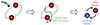 |
Fig. 21. Fly-by in an unstable triple system. The binary system of two massive slow rotators (red) captured a lower mass star (green) that interacted in a close fly-by with one of the massive stars before being ejected. The spin of the closely flown-by star may be increased a bit (blue). |
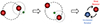 |
Fig. 22. Swallowing of a low-mass star in a triple system: A low-mass star (green) initially moves in the gravitational field of a wide high-mass binary with two slow rotators (red). When the orbit of the low-mass star is disturbed, it spirals on to one of the high-mass components. The resulting post-merger star has an increased mass and spin (blue). |
Each of the four scenarios has its advantages and drawbacks. We suggest that there is no simple best scenario applying for all wide SB2s, rather each SB2 may be best explained by one of the scenarios, and all four scenarios are needed to explain the spin-ups in the entire sample.
We focus the further discussion on the swallowing scenario (item 4 above). It appears plausible, but it depends on the existence of low-mass companions that are at least 8 mag fainter than O stars and can hardly be detected by observations. The short main sequence (MS) time of O stars is similar to the time which low-mass (solar mass) stars need to reach the zero-age main sequence. Thus, the question follows of whether O stars can be surrounded by solar mass stars. We find three arguments supporting that this is indeed probable:
-
(1)
The fragmentation of a large disk (or cloud) around an O-star leads to substructures (Fig. 23). These start to form lower mass stars, say an A0-star with final MS mass of 2 M⊙. When the O star finished accretion and its radiation/wind blows off the parental cloud and disk, then the mass accretion of the A-star has not yet completed. However, the parental cloud and disk is blown away too, leading to cease further mass accretion. This results in a “truncated” A-star with a mass which is presumably a factor of 2–3 lower than the final MS mass. So far, simulations (cf. scenario 1 above) and observations reach bright companions, but with better sensitivity and resolution faint companions should become detectable.
-
(2)
About 40% of B-type stars are SB1 systems (e.g. Chini et al. 2012; a re-investigation of the same sample using additional spectra yields 52% SB1s, Symietz 2024). They have a mass between 3 and 18 M⊙. For SB1 companions, one expects M2 ≈ 0.1 ⋅ M1 of the host star, so that M2 lies in the range of the sought-for low-mass stars. This shows that solar mass stars likely exist around B stars. Since O and B stars are seen mostly in common clusters or star forming regions, it is likely that also O stars are surrounded by solar mass stars.
-
(3)
If indeed several merging events with low-mass stars are at work for O-type stars, then it is possible that the MS time of an O star is also prolonged as it rejuvenates with every merging event (e.g. de Mink et al. 2013). In this case, “coeval” O stars and solar mass stars can exist.
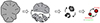 |
Fig. 23. Fragmentation of a cloud or disk into three cores of different size and mass. They form three stars (or proto-stars) of high, medium, and low mass, respectively. During subsequent evolution, the stars interact and merge. |
To conclude, the likelihood for (many) low-mass stars around an O star is high, also indicated by Initial Mass Functions.
Bally & Zinnecker (2005) suggested that two effects can increase the probability of a merging event. Gravitational focusing describes the effect that the true cross section for interactions is much larger than only the projected area of the star. Disk-assisted protostellar capture can further increase the cross section of interaction. The merging event itself is expected to be a very fast process.
The timescale problem for merging/swallowing may be further alleviated, if the configuration of the triple system is already founded before the stars reached the main sequence (Fig. 23). If the triple is already present in an earlier cloud/disk era of the stars, this shortens the overall time needed to achieve the merging.
Bonnell et al. (2001) proposed the “competitive accretion” model. It explains the stellar mass spectrum of a cluster, as well as the fact that high-mass stars gain mass as they gain companions, implying a direct causal relationship between the cluster formation process and the formation of higher-mass stars therein. We note that the accretion processes take place before the stars reach the main sequence. The low-mass merging scenario does not question the competitive accretion model. Rather it provides a valuable additive mechanism during a later evolutionary phase.
To summarise, the post-merger scenario involving the merging of low-mass stars (“swallowing”) has remarkable advantages. In principle, the spin-up is not limited. Swallowing can explain the wide range from slow to fast rotators in wide SB2 systems. For a given input angular momentum by the captured low-mass star the spin-up of the host star increases with declining mass of the host star. Thus, swallowing can naturally explain why mostly the less massive secondary rotates faster then the primary. Swallowing likely reduces the timescale problem of merging of high-mass stars. The interplay/combination with cloud/disk fragmentation is likely and efficient. The existence of low-mass stars “co-eval” with the O star is probable.
As an outlook we note: If the swallowing scenario substantiates, it can indeed help to answer a fundamental question of massive star formation (Zinnecker & Yorke 2007), as it supports the hypothesis that massive stars are grown by the merger of low-mass with medium-mass stars (Bonnell et al. 1998). The progenitor medium-mass stars may be formed by accretion or by merging of several low-mass components.
5.4. Comparison of wide binaries with single stars
The fraction of giants is larger in Cs (57%) than in wide SB2s (32%). Part of the difference could be an observational bias. Giants are more luminous than dwarfs impeding the detection of a companion. We do not follow up on at that here.
Wide binaries (P+S combined9) and C-stars show a similar fraction of slow, medium and fast rotators. This suggests that most C-stars are intrinsically similar to components of (very) wide binaries or of binaries with a (very) small mass ratio M2/M1, both beyond detectability.
In detail, there are some differences, for instance: the fraction of fast rotators among wide binaries (11%) is lower than that of Cs (15%). However, about 50% of the single fast rotators are runaways assumed to be post-interaction binary products (Britavskiy et al. 2023, their Fig. 9). These are rather evolved “old” stars (> 5 Myr) but the wide binaries are almost all “young” (< 5 Myr). We want to compare only matched samples (i.e. young stars) here. By removing the “old” runaway stars (i.e. the 50% above), the fraction of young single fast rotators reduces from 15% to about 7.5%, slightly below that of the wide SB2s.
Does a comparison with the Cs favour or discard one of the 4 spin-up mechanisms proposed for wide binaries? We consider how far these (and other small) statistical differences are consistent with the spin-up scenarios:
-
(1)
The binary stars are born with different spins: If this scenario is true, then we assume that also singles stars are born with a broad range of spins. As long as the stars are young and did not suffer from magnetic braking or momentum loss through winds during the star’s ageing, the v sin i distribution and the fraction of fast rotators should be equal (similar) for wide binaries and single stars, consistent with the data.
-
(2)
Hidden SB1 in a hierarchical triple system: for a single star, this spin-up mechanism reduces to spin-orbit synchronisation in a close SB1 which is undetected (likely due to a very low mass ratio) and appears therefore as C. At the moment, the comparison of wide SB2s with Cs does not reject this mechanism.
-
(3)
Fly-by event: for a single star this spin-up mechanism reduced to a very unlikely rare fly-by of another star. As for wide binaries, this mechanism might play a minor role.
-
(4)
The low-mass merger scenario requires that the orbit of the low-mass star is strongly disturbed. In a binary the massive companion is an ideal disturber. However, a single star lacks that massive disturber, suggesting that Cs have fewer spun-up rotators than wide SB2s. In principle, the presence of another low-mass star may be sufficient to disturb the orbit, but the effect is weaker. Then, part of the Cs can be spun-up in a similar manner as the wide SB2s. Some of the fast rotators Cs are indeed the merge of two massive stars, and they are older but appear rejuvenated after the merger (Schneider et al. 2014; Wang et al. 2020).
To conclude, the v sin i distributions of wide binaries and Cs appear consistent with all 4 spin-up scenarios, not allowing us to reject a scenario.
6. Summary and conclusions
We determined the projected rotational velocity (v sin i) of 238 southern O stars selected from the Galactic O-star Survey. The sample contains 130 spectroscopic single stars (C), 36 single-lined binaries (SB1s), 64 SB2s, and 8 SB3 systems. We carefully applied the Fourier method to high-resolution spectra taken with BESO at Cerro Murphy and supplemented by archival spectra. New results were obtained, in particular for the double-lined binaries (SB2s, including SB3s):
-
(1)
The overall v sin i statistics peaks at slow rotators (40–100 km/s) with a tail towards medium (100–200 km/s) and fast (200–400 km/s) rotators. The medium rotators are four times more frequent in binaries than in single stars. Fast rotators are more frequent in single stars. These results are likely intrinsic and not mimicked by inclination effects. We take slow rotation as a standard against which we compare any cases of increased rotation (> 100 km/s).
-
(2)
For 70 SB2s the orbital periods Porb are known, allowing us to explore the relation between rotation and binary separation. The v sin i distributions differ for close (Porb < 10 d) and wide SB2s (10 d < Porb < 3700 d) and for primaries and secondaries:
-
(a)
For the 29 close SB2s, both primaries and secondaries show a spin-up with respect to slow rotators, and for most binaries the secondary spins faster than the primary (in terms of angular velocity). The spin-up is well explained by a combination of both spin-orbit synchronisation and mass transfer (Roche-lobe overflow, RLOF). This is particularly demonstrated for a subsample of 53 SB2s with known orbit inclination where almost all components rotate with equatorial velocity veq > 100 km/s.
-
(b)
For the 39 wide SB2s, the overall v sin i distribution appears similar to that of single stars (Cs), but primaries differ from secondaries. Mostly, the primary is a slow rotator (75%), but 25% are medium and fast rotators. Mostly, the secondary (∼75%) rotates faster than the primary. A high fraction (43%) of the secondaries are medium and fast rotators. To explain the increased rotation in both primaries and secondaries, mechanisms like spin-orbit synchronisation, RLOF mass transfer, and captured wind material cannot be applied and do not work (at least for Porb ≳ 30 d).
-
(a)
-
(3)
We discussed possible spin-up scenarios for the wide SB2s:
-
(A)
The stars are simply born with different spins. Fragmentation of the birth cloud or the disk may have formed (proto)-stars with different spin. However, it is puzzling why mostly the secondary rotates faster than the primary, and why single stars lack the increased rotation seen in the secondaries.
-
(B)
One (or both) of the massive binary components is a hidden close SB1 in a hierarchical triple (or multiple) system. The short period suggests ongoing spin-orbit synchronisation and mass transfer. Our sample contains two examples, yet they do not exhibit a remarkable spin-up. This brings into question whether this scenario plays a major role.
-
(C)
One of the two massive components was spun-up by a fly-by of an ejected third star in an unstable triple system. It is unclear whether a fly-by transfers enough angular momentum to the massive star. Many such events might be required. Therefore, statistically this mechanism might play a minor role.
-
(D)
Post-merger: In this picture, the increased rotator was spun-up by a merging event in the past. However, a scenario in which two high-mass stars merge and afterwards find a new massive companion to form a new wide SB2 probably requires time frame that is too large and that exceeds the young age of our O stars. Two ways (or a combination of them) alleviate the timescale problem:
-
(a)
The capture and merging (swallowing) of low-mass stars (M ≲ 1 M⊙) is very efficient and explains why the secondary mostly rotates faster than the primary.
-
(b)
The basics of the triple system are already founded before the stars reached the main sequence, in an earlier cloud or disk era of the stars. This shortens the overall time needed to achieve the merging.
-
(a)
This leads us to conclude that the spin-up of wide O binaries is best explained by a combination of disk fragmentation, which lays the basis of the triple, and the subsequent swallowing of low-mass by higher-mass (proto)-stars.
-
(A)
-
(4)
If the swallowing of low-mass stars substantiates, then (in adition to accretion) the formation of high-mass stars benefits from merging.
The rotation rate of the binary components indeed provides valuable insights to early star formation processes.
Data availability
Tables D.1–D.4 are available at the CDS via anonymous ftp to cdsarc.cds.unistra.fr (130.79.128.5) or via https://cdsarc.cds.unistra.fr/viz-bin/cat/J/A+A/692/A192
Cerro Murphy is a subsidiary summit of Cerro Armazones in the Chilean Atacama desert. Since 2020 the observatory is run by the Nikolaus Kopernikus Center, Warsaw, Poland. Hosted within ESO’s Paranal Observatory, its name is Rolf Chini Cerro Murphy Observatory.
Typical ratios v sin i/FWHM lie in a valid range between 0.3 and 0.7, as we derived from modelled line profiles of rotating stars with turbulence. For the secondary we obtain: v sin i/FWHM = 139/169 = 0.82 (wiggles included) which lies outside the valid range and v sin i/FWHM = 119/169 = 0.7 (wiggles excluded) inside the valid range.
The error comparison of the He II lines is similar to that of the He I lines. For O III we have only one line at 5592 Å.
We find that v sin i obtained for He I 4471 is consistent with that for other He I lines. It turns out that wings in He I 4471 have little influence on the determination of v sin i, when using the mirroring technique.
Seven of the 8 SB3 systems host a close P-S pair. The tertiaries (associated with a close P-S pair) have a long period, if measured, or a small RV amplitude indicating a large separation. The tertiaries are not included in the analysis.
The models predict a surprisingly smooth braking curve over time. However, a massive star exhibits line profile variations indicating irregular episodes of strong winds and/or re-arrangement of internal angular momentum. As a promising future step for the models, we suggest to include stochastic mass loss episodes.
The statistical balance between capture probability Pcap and spin gain gspin is controlled by (1) the spatial distribution of tertiaries Cs relative to A and B, (2) a higher likelyhood that the more massive primary wins the capture competition (Pcap ∝ M), and (3) a higher spin gain for the less massive secondary (gspin ∝ 1/(MR2), with mass M and radius R of A and B). Details are beyond the scope of this paper.
If P and S were not gravitationally bound, then each would be a single star, and therefore we use the statistics for P+S combined.
HARPS has a spectral resolution R ∼ 100000, twice that of BESO, FEROS, UVES and Elodie. To keep our sample homogeneous, we did not use HARPS spectra here.
For each bin of width 1 km/s at velocity v_bin the distribution of panel C is scaled from 100 km/s to v_bin (this is illustrated by the thin black curves at 100 km/s and 200 km/s). Then these distributions are coadded, yielding the observed histogram for v sin i (blue).
Acknowledgments
The start of the young massive stars project was funded by the Akademie der Wissenschaften und der Künste Nord-Rhein-Westfalen, Germany. This work was supported by the Deutsche Forschungsgemeinschaft, DFG project number CH71/33-1. This research uses data obtained from the ESO Science Archive Facility and the ELODIE archive at Observatoire de Haute-Provence (OHP). This research has also made use of the SIMBAD database, operated at the CDS, Strasbourg, France. Most of the early BESO spectra were taken and optimised with endurance by Vera Hoffmeister. Anita Nasseri and Noemi Roggero helped with the FEROS and BESO pipelines. We thank Petr Hamanec, Hans Zinnecker and Gonzalo Holgado for fruitful discussions and the anonymous referee for plenty of constructive suggestions.
References
- Abdul-Masih, M. 2023, A&A, 669, L11 [NASA ADS] [CrossRef] [EDP Sciences] [Google Scholar]
- Aerts, C., Simón-Díaz, S., Groot, P. J., & Degroote, P. 2014, A&A, 569, A118 [NASA ADS] [CrossRef] [EDP Sciences] [Google Scholar]
- Ahmadi, A., Beuther, H., Bosco, F., et al. 2023, A&A, 677, A171 [NASA ADS] [CrossRef] [EDP Sciences] [Google Scholar]
- Albacete Colombo, J. F., Morrell, N. I., Rauw, G., et al. 2002, MNRAS, 336, 1099 [NASA ADS] [CrossRef] [Google Scholar]
- Bagnuolo, W. G., Jr., Gies, D. R., & Wiggs, M. S. 1992, ApJ, 385, 708 [NASA ADS] [CrossRef] [Google Scholar]
- Bally, J., & Zinnecker, H. 2005, AJ, 129, 2281 [NASA ADS] [CrossRef] [Google Scholar]
- Baranne, A., Queloz, D., Mayor, M., et al. 1996, A&AS, 119, 373 [NASA ADS] [CrossRef] [EDP Sciences] [Google Scholar]
- Barbá, R. H., Gamen, R., Arias, J. I., et al. 2010, Rev. Mex. Astron. Astrofis. Conf. Ser., 38, 30 [Google Scholar]
- Barbá, R. H., Sabín-Sanjulián, C., Arias, J. I., et al. 2020, MNRAS, 494, 3937 [CrossRef] [Google Scholar]
- Bonnell, I. A., Bate, M. R., & Zinnecker, H. 1998, MNRAS, 298, 93 [Google Scholar]
- Bonnell, I. A., Bate, M. R., Clarke, C. J., & Pringle, J. E. 2001, MNRAS, 323, 785 [Google Scholar]
- Britavskiy, N., Simón-Díaz, S., Holgado, G., et al. 2023, A&A, 672, A22 [NASA ADS] [CrossRef] [EDP Sciences] [Google Scholar]
- Brott, I., de Mink, S. E., Cantiello, M., et al. 2011, A&A, 530, A115 [NASA ADS] [CrossRef] [EDP Sciences] [Google Scholar]
- Campillay, A. R., Arias, J. I., Barbá, R. H., et al. 2019, MNRAS, 484, 2137 [Google Scholar]
- Carroll, J. A. 1933, MNRAS, 93, 478 [NASA ADS] [CrossRef] [Google Scholar]
- Chini, R., Hoffmeister, V., Kimeswenger, S., et al. 2004, Nature, 429, 155 [NASA ADS] [CrossRef] [Google Scholar]
- Chini, R., Hoffmeister, V. H., Nasseri, A., Stahl, O., & Zinnecker, H. 2012, MNRAS, 424, 1925 [Google Scholar]
- Conti, P. S., & Alschuler, W. R. 1971, ApJ, 170, 325 [NASA ADS] [CrossRef] [Google Scholar]
- Conti, P. S., & Ebbets, D. 1977, ApJ, 213, 438 [CrossRef] [Google Scholar]
- de Mink, S. E., Langer, N., Izzard, R. G., Sana, H., & de Koter, A. 2013, ApJ, 764, 166 [Google Scholar]
- de Mink, S. E., Sana, H., Langer, N., Izzard, R. G., & Schneider, F. R. N. 2014, ApJ, 782, 7 [Google Scholar]
- Dekker, H., D’Odorico, S., Kaufer, A., Delabre, B., & Kotzlowski, H. 2000, SPIE Conf. Ser., 4008, 534 [Google Scholar]
- Eggleton, P. P. 1983, ApJ, 268, 368 [Google Scholar]
- Ekström, S., Georgy, C., Eggenberger, P., et al. 2012, A&A, 537, A146 [Google Scholar]
- Ekström, S., Meynet, G., Georgy, C., et al. 2020, in Stars and their Variability Observed from Space, eds. C. Neiner, W. W. Weiss, D. Baade, et al., 223 [Google Scholar]
- Evans, C. J., Taylor, W. D., Hénault-Brunet, V., et al. 2011, A&A, 530, A108 [NASA ADS] [CrossRef] [EDP Sciences] [Google Scholar]
- Fuhrmann, K., Chini, R., Hoffmeister, V. H., et al. 2011, MNRAS, 411, 2311 [NASA ADS] [CrossRef] [Google Scholar]
- Gray, D. F. 1973, ApJ, 184, 461 [CrossRef] [Google Scholar]
- Gray, D. F. 2005, The Observation and Analysis of Stellar Photospheres (UK: Cambridge University Press) [Google Scholar]
- Holgado, G., Simón-Díaz, S., Haemmerlé, L., et al. 2020, A&A, 638, A157 [NASA ADS] [CrossRef] [EDP Sciences] [Google Scholar]
- Holgado, G., Simón-Díaz, S., Herrero, A., & Barbá, R. H. 2022, A&A, 665, A150 [NASA ADS] [CrossRef] [EDP Sciences] [Google Scholar]
- Howarth, I. D., & Prinja, R. K. 1989, ApJS, 69, 527 [NASA ADS] [CrossRef] [Google Scholar]
- Howarth, I. D., Siebert, K. W., Hussain, G. A. J., & Prinja, R. K. 1997, VizieR Online Data Catalog: J/MNRAS/284/265 [Google Scholar]
- Kaufer, A., Wolf, B., Andersen, J., & Pasquini, L. 1997, Messenger, 89, 1 [NASA ADS] [Google Scholar]
- Kaufer, A., Stahl, O., Tubbesing, S., et al. 1999, Messenger, 95, 8 [Google Scholar]
- Kriz, S., & Harmanec, P. 1975, Bull. Astron. Inst. Czechosl., 26, 65 [NASA ADS] [Google Scholar]
- Krumholz, M. R., Klein, R. I., McKee, C. F., Offner, S. S. R., & Cunningham, A. J. 2009, Science, 323, 754 [Google Scholar]
- Kudritzki, R.-P., & Puls, J. 2000, ARA&A, 38, 613 [Google Scholar]
- Langer, N. 2012, ARA&A, 50, 107 [CrossRef] [Google Scholar]
- Lanz, T., & Hubeny, I. 2003, ApJS, 146, 417 [NASA ADS] [CrossRef] [Google Scholar]
- Linder, N., Rauw, G., Sana, H., De Becker, M., & Gosset, E. 2007, A&A, 474, 193 [NASA ADS] [CrossRef] [EDP Sciences] [Google Scholar]
- Linder, N., Rauw, G., Martins, F., et al. 2008, A&A, 489, 713 [NASA ADS] [CrossRef] [EDP Sciences] [Google Scholar]
- Maeder, A. 2009, Physics, Formation and Evolution of Rotating Stars (Springer Berlin Heidelberg) [Google Scholar]
- Maeder, A., & Meynet, G. 2000, ARA&A, 38, 143 [Google Scholar]
- Mahy, L., Sana, H., Shenar, T., et al. 2022, A&A, 664, A159 [NASA ADS] [CrossRef] [EDP Sciences] [Google Scholar]
- Maíz-Apellániz, J., Walborn, N. R., Galué, H. Á., & Wei, L. H. 2004, ApJS, 151, 103 [CrossRef] [Google Scholar]
- Maíz Apellániz, J., Úbeda, L., Barbá, R. H., et al. 2015, Highlights of Spanish Astrophysics VIII, 604 [Google Scholar]
- Maíz Apellániz, J., Sota, A., Arias, J. I., et al. 2016, ApJS, 224, 4 [CrossRef] [Google Scholar]
- Maíz Apellániz, J., Sana, H., Barbá, R. H., Le Bouquin, J. B., & Gamen, R. C. 2017, MNRAS, 464, 3561 [Google Scholar]
- Martins, F. 2018, A&A, 616, A135 [NASA ADS] [CrossRef] [EDP Sciences] [Google Scholar]
- Martins, F., Schaerer, D., Hillier, D. J., & Heydari-Malayeri, M. 2004, A&A, 420, 1087 [NASA ADS] [CrossRef] [EDP Sciences] [Google Scholar]
- Martins, F., Schaerer, D., Hillier, D. J., et al. 2005a, A&A, 441, 735 [NASA ADS] [CrossRef] [EDP Sciences] [Google Scholar]
- Martins, F., Schaerer, D., & Hillier, D. J. 2005b, A&A, 436, 1049 [NASA ADS] [CrossRef] [EDP Sciences] [Google Scholar]
- Mayer, P., Drechsel, H., & Irrgang, A. 2014a, A&A, 565, A86 [NASA ADS] [CrossRef] [EDP Sciences] [Google Scholar]
- Mayer, P., Harmanec, P., Sana, H., & Le Bouquin, J.-B. 2014b, AJ, 148, 114 [NASA ADS] [CrossRef] [Google Scholar]
- Mayer, P., Harmanec, P., Chini, R., et al. 2017, A&A, 600, A33 [NASA ADS] [CrossRef] [EDP Sciences] [Google Scholar]
- Nasseri, A., Chini, R., Harmanec, P., et al. 2014, A&A, 568, A94 [NASA ADS] [CrossRef] [EDP Sciences] [Google Scholar]
- Oliva, G. A., & Kuiper, R. 2020, A&A, 644, A41 [NASA ADS] [CrossRef] [EDP Sciences] [Google Scholar]
- Packet, W. 1981, A&A, 102, 17 [NASA ADS] [Google Scholar]
- Penny, L. R. 1996, ApJ, 463, 737 [Google Scholar]
- Penny, L. R., Seyle, D., Gies, D. R., et al. 2001, ApJ, 548, 889 [NASA ADS] [CrossRef] [Google Scholar]
- Penny, L. R., Gies, D. R., Wise, J. H., Stickland, D. J., & Lloyd, C. 2002, ApJ, 575, 1050 [NASA ADS] [CrossRef] [Google Scholar]
- Puls, J., Urbaneja, M. A., Venero, R., et al. 2005, A&A, 435, 669 [NASA ADS] [CrossRef] [EDP Sciences] [Google Scholar]
- Putkuri, C., Gamen, R., Morrell, N. I., et al. 2018, A&A, 618, A174 [NASA ADS] [CrossRef] [EDP Sciences] [Google Scholar]
- Putkuri, C., Gamen, R., Morrell, N. I., et al. 2021, A&A, 650, A96 [NASA ADS] [CrossRef] [EDP Sciences] [Google Scholar]
- Ramírez-Agudelo, O. H., Simón-Díaz, S., Sana, H., et al. 2013, A&A, 560, A29 [NASA ADS] [CrossRef] [EDP Sciences] [Google Scholar]
- Ramírez-Agudelo, O. H., Sana, H., de Mink, S. E., et al. 2015, A&A, 580, A92 [NASA ADS] [CrossRef] [EDP Sciences] [Google Scholar]
- Raucq, F., Rauw, G., Gosset, E., et al. 2016, A&A, 588, A10 [NASA ADS] [CrossRef] [EDP Sciences] [Google Scholar]
- Rauw, G., Sana, H., Antokhin, I. I., et al. 2001a, MNRAS, 326, 1149 [NASA ADS] [CrossRef] [Google Scholar]
- Rauw, G., Nazé, Y., Carrier, F., et al. 2001b, A&A, 368, 212 [NASA ADS] [CrossRef] [EDP Sciences] [Google Scholar]
- Rauw, G., Vreux, J. M., Stevens, I. R., et al. 2002, A&A, 388, 552 [NASA ADS] [CrossRef] [EDP Sciences] [Google Scholar]
- Rivero González, J. G., Puls, J., Najarro, F., & Brott, I. 2012, A&A, 537, A79 [NASA ADS] [CrossRef] [EDP Sciences] [Google Scholar]
- Rosu, S., Rauw, G., Farnir, M., Dupret, M. A., & Noels, A. 2022, A&A, 660, A120 [NASA ADS] [CrossRef] [EDP Sciences] [Google Scholar]
- Royer, F. 2005, Mem. Soc. Astron. Ital. Suppl., 8, 124 [Google Scholar]
- Ryans, R. S. I., Dufton, P. L., Rolleston, W. R. J., et al. 2002, MNRAS, 336, 577 [Google Scholar]
- Sahade, J. 1959, PASP, 71, 151 [NASA ADS] [CrossRef] [Google Scholar]
- Sana, H., Nazé, Y., O’Donnell, B., Rauw, G., & Gosset, E. 2008a, New Astron., 13, 202 [Google Scholar]
- Sana, H., Gosset, E., Nazé, Y., Rauw, G., & Linder, N. 2008b, MNRAS, 386, 447 [Google Scholar]
- Sana, H., de Mink, S. E., de Koter, A., et al. 2012, Science, 337, 444 [Google Scholar]
- Sana, H., de Koter, A., de Mink, S. E., et al. 2013, A&A, 550, A107 [NASA ADS] [CrossRef] [EDP Sciences] [Google Scholar]
- Sana, H., Abdul-Masih, M., Banyard, G., et al. 2022, arXiv e-prints [arXiv:2209.06287] [Google Scholar]
- Schneider, F. R. N., Izzard, R. G., de Mink, S. E., et al. 2014, ApJ, 780, 117 [Google Scholar]
- Shenar, T., Sana, H., Mahy, L., et al. 2022, A&A, 665, A148 [NASA ADS] [CrossRef] [EDP Sciences] [Google Scholar]
- Simón-Díaz, S., & Herrero, A. 2007, A&A, 468, 1063 [NASA ADS] [CrossRef] [EDP Sciences] [Google Scholar]
- Simón-Díaz, S., & Herrero, A. 2014, A&A, 562, A135 [NASA ADS] [CrossRef] [EDP Sciences] [Google Scholar]
- Simón-Díaz, S., Godart, M., Castro, N., et al. 2017, A&A, 597, A22 [CrossRef] [EDP Sciences] [Google Scholar]
- Slettebak, A. 1956, ApJ, 124, 173 [NASA ADS] [CrossRef] [Google Scholar]
- Sota, A., Maíz Apellániz, J., Walborn, N. R., & Shida, R. Y. 2008, Rev. Mex. Astron. Astrofis. Conf. Ser., 33, 56 [NASA ADS] [Google Scholar]
- Sota, A., Maíz Apellániz, J., Walborn, N. R., et al. 2011, ApJS, 193, 24 [Google Scholar]
- Sota, A., Maíz Apellániz, J., Morrell, N. I., et al. 2014, ApJS, 211, 10 [Google Scholar]
- Stahl, O., Kaufer, A., & Tubbesing, S. 1999, ASP Conf. Ser., 188, 331 [NASA ADS] [Google Scholar]
- Struve, O. 1937, ApJ, 85, 41 [NASA ADS] [CrossRef] [Google Scholar]
- Sundqvist, J. O., Simón-Díaz, S., Puls, J., & Markova, N. 2013, A&A, 559, L10 [NASA ADS] [CrossRef] [EDP Sciences] [Google Scholar]
- Symietz, F. 2024, Doctoral Thesis, Ruhr-Universität Bochum, Germany [Google Scholar]
- Tassoul, M., & Tassoul, J.-L. 1997, ApJ, 481, 363 [Google Scholar]
- Vink, J. S. 2022, ARA&A, 60, 203 [NASA ADS] [CrossRef] [Google Scholar]
- Wang, C., Langer, N., Schootemeijer, A., et al. 2020, ApJ, 888, L12 [NASA ADS] [CrossRef] [Google Scholar]
- Wellstein, S. 2001, Ph.D. Thesis, University of Potsdam, Germany [Google Scholar]
- Zahn, J. P. 1975, A&A, 41, 329 [NASA ADS] [Google Scholar]
- Zahn, J. P. 1977, A&A, 57, 383 [Google Scholar]
- Zasche, P., Henzl, Z., & Mašek, M. 2022, A&A, 664, A96 [NASA ADS] [CrossRef] [EDP Sciences] [Google Scholar]
- Zhang, Y., Tan, J. C., Tanaka, K. E. I., et al. 2019, Nat. Astron., 3, 517 [NASA ADS] [CrossRef] [Google Scholar]
- Zinnecker, H., & Yorke, H. W. 2007, ARA&A, 45, 481 [Google Scholar]
Appendix A: Disentangling SB2 and SB3 line profiles
We disentangled the components of SB2/SB3 systems using a decomposition of the observed profiles into 2-3 Gaussian profiles. The line profile of one component is then obtained after subtracting the Gaussian fit of the complementary component(s) from the entire observed line profile.
In more detail, the line profiles of single O stars are to first order well approximated by a Gaussian function. Small deviations are due to the fact that the line shape is rounder for a rotation-dominated star and more triangular with Lorentzian wings for a turbulence-dominated star (e.g. Simón-Díaz et al. 2017). For the chi square minimising Gaussian fit, we used the SIMPLEX algorithm with a suite of starting parameters in order to avoid false local chi square minima. For a given line, we first determined the parameters of the Gaussian profiles for those spectra, where individual line profiles were best separated in RV. Whenever it was possible, we then kept these parameters fixed and changed only the RV of individual profiles to get the best fit. However, when keeping width and height fixed, this often leads to uncomfortable residuals in the resulting decomposed line profiles. The residuals become worse for small dRV between the components. The residuals may affect the v sin i determination. The technique with fixed Gaussian widths and heights for all spectra is widely used to determine RV curves (e.g. Mayer et al. 2017; problems near conjunction are discussed in Rosu et al. 2022). However, our aim here is slightly different from the determination of RV curves, since we are seeking for a best removal of the complementary component(s). Therefore, we did not keep width and height fixed for all spectra. Exceptions are a few very faint companions, where a fixed width and/or height stabilised the fit. Rather in most cases, we fit each spectrum individually with free parameters, and then rejected outliers (typically those spectra with small dRV). In the net effect, we used only those (mostly 2-7) spectra with best separated components.
Binaries with narrow components are easier resolved than with broad components. To account for this, we quantify the separation of the components A and B relative to their mean width, avgFWHM = (FWHM(A) + FWHM(B))/2, via the dimensionless number:
 (A.1)
(A.1)
In addition to Sep, we take into account the depth (i.e. Gaussian height) of the components. In a given spectrum with constant noise level, a deep component allows for a better fit than a flat component. Overall, the quality of the disentangling may affect the quality of the v sin i determination. Therefore, we assigned a quality flag QF to each SB2/SB3 component, based on visual inspection of the spectra, Sep and the component depths: high (QF=A), medium (B) and low (C). For each QF we estimate a likely uncertainty of v sin i of about 10% (A), 20% (B) and 30% (C). Further details on the errors are given in Sect. 3.2.4.
We group the typical observed line shapes into 8 disentangling types (DT). They cover the range of separation, line width (narrow and broad), and height (faint and flat, or bright and sharp) of our sample. Examples for the 8 DTs are depicted in Fig. A.1. They include the best and worst cases for SB2s (DT 1-6) and SB3s (DT 7-8). The next subsections describe the 8 DTs, followed by a summary of the disentangling (Sect. A.9). Primaries, Secondaries and Tertiaries are abbreviated by P, S and T. All plots mentioned refer to the panel blocks in Fig. A.1.
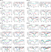 |
Fig. A.1. Examples of disentangling types (DT) for SB2s (DT 1-6) and SB3s (DT 7-8). Details are described in Sect. A. Radial velocities “v” are as observed and not corrected for systemic velocities. |
A.1. DT 1
HD 075759, two isolated components with wide separation, one of the best examples. From the 30 available spectra (i.e. epochs) we show only the best one.
Left panel: Both components are seen in O III and He II, hence are O-Stars (we determined spectral types O9 IV and O9.5 V; previous studies have reported O9 V and B0 V, e.g. Sota et al. 2014; Holgado et al. 2020).
Right panel: The profiles are well fit by Gaussian functions. Subtracting Gaussian fits results in negligible residual wiggles with amplitude < 3% of the profile depths. The residuals are about/below the noise level. Therefore, their effect on the v sin i determination is negligible.
We assign QF = A to both components P and S.
A.2. DT 2
HD 117856, two components of similar width with wide separation (Sep = 1.4) but slightly overlapping in RV. This is still a very good example. The important feature of the observed profiles is the clear dip seen between the two components (in the Helium lines). The dip constrains the Gaussian decomposition, yielding two components of similar width. From the 11 available spectra we here show only the best one.
Left panel: The secondary is barely seen in O III but both components are well seen in He II 4686 (as well as He II 4541 and 5411 with broader profiles not shown here). This argues for O-type stars (not B-stars) and we determined spectral types O9.5 III and O9.7 V for P and S, respectively.
Right panel: The profiles are well fit by Gaussian functions. Gaussian decomposition results in negligible residual wiggles, suggesting no influence on the v sin i determination.
We assign QF = A to both components.
A.3. DT 3
HD 168075, still a good example, two resolved components of similar width with small separation (Sep ≈ 1.1). The line profiles strongly overlap in velocity. The secondary is relatively faint and produces only a wing in the He lines without dip. The wing is exclusively one-sided (sometimes left, sometimes right). We show 2 of the 10 available spectra.
2006-Aug-21: In O III, the companion is "isolated" by a dip in the observed line profile. He I 5876 shows a clear wing of a companion right-hand of P. The He II 4686 line is generally broader leading to a small asymmetry to the right.
2004-May-07: near conjuction (dRV close to 0 and the joint profile depth lies near the maximum). O III appears quite symmetric, He I and He II show a very small asymmetry to the left.
Gaussian decomposition was performed using free parameters (height, width, position) for P, but for S we kept height and/or width fixed with some tolerance (after examining the range for suited height and width). The width of P and S, respectively, differs between the two spectra by about 10%. We have allowed for this difference, to keep the residuals small. Indeed, for both spectra, the residuals lie within the noise suggesting no influence on the v sin i determination.
We assign QF = A and B to P and S, respectively.
Note: already these two spectra reject the possibility that the right tail seen on 2006-Aug-21 is due to a broad S with a narrow P on top. Furthermore, from Gaussian decomposition of the 10 available spectra we were able to reproduce the orbital elements, period (∼43.6 d Barbá et al. 2010; Sota et al. 2014) as well as K1 ≈ 35 km/s and K2 ≈ 70 km/s. This supports the correctness of the Gaussian decomposition and that both components have similar (narrow) width.
We identified 6 SB2s of DT 3. They have between 9 and 50 spectra available. Near conjunction, all these SB2s lack the two-sided wing indicating a broad S (an exception may be HD 153426; see below). This gives us confidence in the decomposition with regard to v sin i.
A.4. DT 4
HD 150135, a narrow primary component overplotted on a broad component is nevertheless a good example. The components largely overlap in velocity and have a very small separation (Sep < 0.8). In the 17 available spectra, the relatively faint S produces only a wing without dip. The wing switches to the opposite RV side of the narrow P (sometimes left, sometimes right) but near conjunction the wing appears simultaneously to both sides. This strongly suggests a broad S.
We show 4 spectra: 2015-Jun-25: clear asymmetry in O III, He I 5876 and He II 4686, suggesting an O-type companion. None of the spectra shows a dip hence the companion is not constrained to be narrow, rather it might be broad.
The next 3 panels show the Gaussian decomposition in He I 5876 using free parameters. It provides evidence for a broad companion:
2007-Apr-21: S left-hand of P, Sep = 0.35.
2009-Feb-20: S right-hand of P, Sep = 0.56.
2013-Jun-25 (S close to P, Sep = 0.19): In this epoch, RV of P lies between the two extremes above, indicating near-conjunction. There, the observed profile exhibits wings on both sides left and right of the narrow P. This (and the absence of a dip at larger dRV) strongly supports a broad S: If S were narrow (similar to P), then only a one-sided wing would be expected.
For most spectra, the residuals from the Gaussian decomposition with free parameters are small. We assign QF(P) = A and QF(S) = B, to account for a few spectra with noticable wiggles for S.
With regard to v sin i, the narrow P and broad S are trustable. Additional evidence for a broad S comes from the spectral types and the orbits:
a) Altogether, from the decomposition of several lines and their EW ratios we estimated spectral types about O6 V and O7 III for P and S, respectively, consistent with spectral type O6.5 V ((f))z reported for the combined system (Sota et al. 2014). We were able to reproduce the known orbital period of 181 d reported by Sota et al. (2014). From the 17 spectra we derived RV curves for both components, yielding a nearly circular orbit with K1 ≈ 60 ± 5 km/s and K2 ≈ 75 ± 10 km/s, hence a mass ratio M2/M1 ≈ 0.8, which is within the uncertainties consistent with that of an O6 + O7 binary (Martins 2018).
b) If we fit S with a narrow (instead of a broad) component, this would result in a noisy RV curve with K2 > 120 km/s, yielding M2/M1 ≈ 0.5. If P has M1 ≈ 28 M⊙ (adopting O6.5 V, Sota et al. 2014), this would imply M2 ≈ 14 M⊙, hence a B-type secondary which would not show O III and He II lines, contrary to the observed spectra.
The examples in DT 3 and DT 4 appear similar by showing wings without a dip, but they differ by the width of the companion (narrow or broad). We have identified 15 DT 4 systems. Based on 9 - 45 available spectra, each DT 4 system shows the switch between one-sided broad wings near maximal dRV and two-sided wings near conjunction.
A.5. DT 5
HD 152219, a prominent broad P and a faint narrower S. It is an example for a poor secondary in our sample, and the only one of this DT. While the components are well discerned by their separation (Sep ≈ 1.6), the brightness ratio is large (P/S ≳ 5). For Gaussian profiles, a large P/S is not harmful as we found in many other cases. In HD 152219, however, the line profile of P is rotation-dominated (i.e. round), and deviates from a Gaussian. The combination of the large brightness ratio and the round shape of P lead to exceptionally large residuals for S.
S is a B-type star (Sana et al. 2008b; Rosu et al. 2022) and neither seen in O III nor He II. Here we show 2 out of 24 spectra in He I 4713, 4922, 5876 (top panel row of the block) on 2004-May-05 and 2006-May-06 (S on the left and right of P, respectively).
Gaussian decomposition using free parameters is shown for He I 4922 (bottom panels of the block). The large brightness ratio leads to strong residual wiggles for S, when subtracting a Gaussian fit of P. The amplitude of the wiggles reaches the depth of S.
As mentioned above, the line profile deviates from a Gaussian, and this difference leads to the residual wiggles. The relative strength of the wiggles depends on the depth ratio (Gaussian height). Therefore P does not receive noticeable wiggles produced by the faint S, but S receives strong wiggles from the bright P.
Notably Sep is sufficiently large, so that the wiggles caused by P lie essentially outside of the profile of S. They do not directly change the (core of the) profile of S. This enables us to essentially reduce the effect of the residuals on the v sin i determination by using a small cut-out window around the profile of S (± 3 × standard deviation ≈ 1.25 × FWHM of S). More details are explained in Sect. 3.2.3.
We assign QF = A and C to P and S, respectively.
A.6. DT 6
CPD −59 2600 has a bright medium-narrow P and a faint broad S, with very small Sep ≲ 0.5. This is the worst and most uncertain SB2 example in our sample. Sota et al. (2014) noted that this system is an O6 V ((f)) SB1 with a 626 d period, and possibly an SB2.
Here we show 2 out of 15 spectra in O III 5592, He I 4471 and He II 4541 (top panels of the block) on 2004-Feb-05 (tail left) and 2008-Jun-10 (tail right). The observed line profiles show a tail to the left and right of P, respectively, but no dip. The tail is also seen in other sufficiently strong lines (He I 4026, 5876 and He II 4686). Whenever visible, the tails are consistent in all lines.
The tail lies at the opposite RV side of P (e.g. if P is on the left, then the tail to the right, vice versa). As for HD 150135 (DT 4), the observed profile appears – near conjunction – more symmetric with two-sided tails left and right of P. This tail behaviour questions a wind as explanation. Rather it suggests the presence of an O-type companion with broad and flat line profile.
The Gaussian decomposition yields consistent results, shown for He I 5876 in the bottom panels of the block in Fig. A.1. After several attempts with free Gaussian parameters, we kept the depth and width of the broad S fixed.
Applying Gaussian decomposition, the known period helped us to derive (noisy) RV curves for P and S. They indicate an eccentric orbit with K1 ≈ 50 km/s, K2 ≈ 75 km/s, and a mass ratio M2/M1 ≈ 0.67. The EW ratios He I4471/He II4541 for P and S are uncertain but consistent with spectral types O6 V and O8 V, respectively, yielding M2/M1 ≈ 0.67. The overall agreements provide further support for the broad S.
v sin i of P is well determined, but S is affected by strong residual noise with an amplitude up to 30% of the profile depth. We assign QF = B and C to P and S, respectively.
A.7. DT 7
DT 7 and DT 8 systems refer to SB3s. DT 7 show two dips allowing us to clearly decompose the three components, but DT 8 have only one dip. While a DT 8 is a clear SB3, it is harder compared to a DT 7 to distinguish between narrow or broad components and more spectra are needed to decompose the three components. In this section we illustrate the DT 7 with two examples (a and b):
a)
CPD −59 2636ABC, this is a very good example for a triple system. Albacete Colombo et al. (2002) found spectral types O7 V, O8 V and a period of 3.6 d for P and S, and a third star T of spectral type O9 V with a 5.03 d period.
Here we show one spectrum out of five. Top panel: in all lines the three components are well separated with a clear dip, reminiscent of DT 2 above. P, S and T are identified via EW ratios of diagnostic lines.
Bottom panel: the Gaussian decomposition yields moderate FWHM for all components, and any residuals lie inside the noise level.
Regarding v sin i, we assign QF = A to each component.
b)
CPD −59 2603, a known hierarchical triple system consisting of a short-period (2.15 d) eclipsing O7 V + O9.5 V binary bound to a B0.2 IV star (Rauw et al. 2001a). Among 10 spectra, it is still a good example with three well isolated components in He I (top panel). However, as for DT 5 above, the bright rotation-dominated round profile of P leads to strong residuals for S and T (bottom panel). Therefore, we assign QF = A, B, and C to P, S and T, respectively.
A.8. DT 8
δ Cir is a known triple consisting of an eclipsing binary O7 III-V + O9.5 V bound to a wide B0.5 V (Penny et al. 2001 based on IUE spectra; Mayer et al. 2014b essentially based on 95 HARPS spectra10). Based on the BESO and FEROS spectra, however, it is a relatively poor SB3 example, because a unique decomposition requires an additional second dip between components which is not seen.
We show two spectra with large dRV out of 16, one with FEROS on 2009-May-02 and a noisier one with BESO on 2009-Aug-28. We consider the He I 4922 spectra: The FEROS spectrum exhibits one clear dip, which reveals S well isolated from P. However, Gaussian decomposition implies a third component T which is poorly constrained between S and P. The BESO spectrum shows two marginal dips, which could be the signatures between P, S and T. However, in other He I lines we see only one dip and He I 4922 could be contaminated by O II 4924.5 as noted by Mayer et al. 2014b. While any residuals appear small, the Gaussian parameters width and height of the resulting components differ between the two different spectra. This holds also for other He I lines. Therefore, we assign QF = B, C, and C to P, S and T, respectively.
A.9. Disentangling summary
Using Gaussian decomposition, we were able to disentangle 62 SB2+SB3 systems (54 SB2 and 8 SB3). The number of systems in the disentangling types are: 18 (DT 1), 13 (DT 2), 6 (DT 3), 15 (DT 4), 1 (DT 5), 1 (DT 6), 4 (DT 7), 4 (DT 8). The DTs cover the range from well resolved pairs to pairs with small separation; they also cover the full range of component width and their peak height. The SB2 decomposition is possible down to very small separation (Sep ∼ 0.5) which is is reached, if a sharply-peaked profile sits on top of a broad flat profile. A larger separation is required (Sep ≳ 1), if the components have similar width and height.
Among our sample, two SB2 systems are of poor disentangling quality (DT 5, DT 6). In addition, two SB2s appear uncertain: HD 125206 (DT 3) could be an SB3, and in HD 153426 (DT 3) the secondary could be even broader (DT 4). In two SB3s, HD 092206 C and δ Cir, we determined v sin i only for P and S, because the tertiary is too noisy/uncertain. We are confident that the disentangling of the vast majority of systems (58/62) allows us to obtain robust v sin i results for P and S.
In addition, we identified 10 SB1s which are reported in the literature as SB2 systems with reliable v sin i for both P and S (Tab. D.2). For the scientific analysis in Sect. 5 we included these 10 systems as SB2s; S is faint and shows mostly a flat broad profile below our detectability. We determined v sin i of P from the total line profile and took v sin i of S from the literature; we assigned DT = 0 and QF (P,S) = (D,N), with a likely uncertainty of v sin i (P) of about 15% (QF=D) and QF=N means “not known”.
Tab. D.2 lists the entire sample of 72 SB2+SB3s together with spectral types and luminosity classes; if they have not been published or differ from previous works, we list those derived by our data and add the reference “this work”. There we also give the disentangling types DT and the quality flags QF for the components.
Appendix B: The effect of a slow wind or an expanding halo on the vsini determination
In a nutshell, an isotropic stellar wind (or an expanding halo) is a priori independent of rotation and turbulence. The wind has to be treated as an additional component Pwind to the line profile such that eq. 1 is expanded as
 (B.1)
(B.1)
We note that Pwind is not part of the mathematical convolution term (eq. 1). A convolution term will not lead to a bias in the v sin i determination; the only exception is that a large vturb leads to a steeply declining FT amplitude and may shift the FT minimum into the noise level biasing v sin i to larger values (see Fig. 2. of Simón-Díaz & Herrero 2007). The problematic issue is that the wind is an additive and asymmetric contribution to the line profile. Any asymmetric profile leads to a complicated behaviour in the Fourier domain and may produce FT minima which are hard to predict.
In more detail, Pwind is composed of an absorption component Pw_abs seen by the observer in front of the stellar disk and an emission component Pw_em surrounding the star
 (B.2)
(B.2)
Pw_abs and Pw_em may be somehow connected, but details are still complicated and subject to intense research. On the modelling side, we note that TLUSTY models (Lanz & Hubeny 2003) are static plane-parallel models with full non-LTE metal line blanketing. They are suitable for O stars that have weak stellar winds. On the other hand, FASTWIND model atmospheres (Puls et al. 2005; Rivero González et al. 2012) are not truly hydrodynamic as the programme does not solve for the wind structure but adopts a wind law.
To illustrate the effect of a wind on the v sin i determination, we assume 1) that both the wind intensity and velocity are low (“weak wind” Martins et al. 2004, 2005a), 2) that both components Pw_abs and Pw_em are optically thin, 3) that the contribution of Pw_em behind the stellar disk is negligible. Notably an isotropic wind emission component Pw_em with constant velocity has a round line profile shape, similar to the shape of a rotating star, and it will likewise produce charactieristic FT minima as well.
To keep the illustration simple, we further assume that the blue absorption wing Pw_abs is absent, so that the line profiles are symmetric and the FT is real (i.e. imaginary part = 0). Such a configuration resembles that of an extended slowly expanding halo with Rhalo > 100 Rstar, where the solid angle for producing the blue absorption wing Pw_abs becomes negligibly small. Figure B.1 shows two model examples, both having vturb = 50 km/s (Lorentz FWHM), vwind = 50 km/s (convolved with a Gaussian, but details on that do not affect the illustration), and Pw_abs contributes 5% to the original line profile:
-
1)
a “null” rotator with v sin i = 0 km/s,
-
2)
a “mid” rotator with v sin i = 100 km/s.
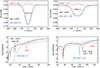 |
Fig. B.1. Effect of the emission of an isotropic slow wind on the line profile (top) and its Fourier transform (FT, bottom), for two rotation speeds v sin i = 0 km/s (“null rotator” left) and v sin i = 100 km/s (“mid rotator” right). Top: The blue solid line shows (1) the rotating star, a rotationally broadened line profile convolved with Lorentzian, vrot = 50 km/s, FWHM vturb = 50 km/s. The red solid line shows (2) an isotropic slow wind halo with vwind = 50 km/s and dispersion ≈ 20 km/s (total FWHM ≈ 65 km/s). The wind strength is 5% of the stellar equivalent width. The dash-dotted black line shows the combined profile of star and wind (sum of (1) and (2)). We note that the combined profile has a rounder (i.e. more boxy) shape than the pure stellar profile. Bottom: FT amplitude of the rotating star (blue), of the wind halo (red), and of the combined profile (star and wind, black). |
We note that FWHM of the wind profile is smaller than FWHM of the stellar profile. The two striking features of the examples are
-
1)
The wind rounds-off the tip of the line profile (top panels).
-
2)
The wind produces FT minima (bottom panels, red), similar to what a rotating star does.
-
3)
For the “null” rotator: at high frequencies (low v sin i on the x-axis) the FT amplitude of the wind exceeds that of the star, because the FWHM of line profile of the wind is smaller than that of the star. As a consequence of this “cross-over” of the FT amplitudes, the combined profile shows high frequency FT minima which are only due to the wind and have little to do with the stellar rotation.
-
4)
For the “mid” rotator, the wind effects are present but much weaker, so that the FT minima of the combined star+wind profile are moderately shifted to lower frequencies (right hand direction in the plot), resulting in a bias of v sin i to about 10% larger values.
The model examples are simple but give us a warning on potential biases when determining v sin i in the presence of a slow wind. For a fast rotating star (vrot ∼ 200 km/s) the line profile is broad and shallow. Then a slow wind emission (of 5% intensity) creates a bump, so that the line profiles mimick a double star and can be rejected for rotational analysis.
We note that both the v sin i artefact and the v sin i bias are not a failure of the FT method. Rather the FT method is particularly sensitive to features affecting the line profile, probably more sensitive than the GOF method. The basic effect of the wind is to round-off the tip of the line profile. If the rounded-off line profile is analysed with the GOF method, a similar v sin i bias will be obtained.
A fast wind (emission component) has a broad line profile and a steeply declining FT amplitude. If the wind’s FWHM is larger than the stellar FWHM, no “cross-over” of the FT amplitudes occurs. Likewise, we note that typically the line profile of a wind absorption component Pw_abs is narrower than the emission component, but blue-shifted. This asymmetry leads to a complicated behaviour of the FT amplitude, spiraling around the origin of the FT plane, but in general no “cross-over” of the FT amplitudes is expected.
For real data, even with simplified assumptions, a proper solution of Eqs. B.1 and B.2 has many free parameters and requires extremely precise spectral line profiles, exceeding the quality of our observational data. For instance, the continuum level next to the line profile exhibits low-frequency noise leading to uncertainties and preventing the required precision.
A detailed treatment and modelling of the wind effects with regard to the determination of v sin i is beyond the frame of this paper; we hope that the examples encourage specialists in the field to find practicable solutions. For our purpose here we keep in mind that a weak wind may bias v sin i of slow+medium rotating stars to larger values. For fast rotators a slow wind produces an easily detectable dip in the line profile, unless the wind intensity is extremely small; for such a weak and slow wind any bias on v sin i might be small (< 10%). The example of the “null” rotator with a slow wind may provide a key to solve the puzzling v sin i results reported by Sundqvist et al. (2013). In addition, if a slow wind is more pronounced in Helium lines compared to metal lines, it may explain (at least partially) why the determined v sin i of slow rotators is often larger for Helium lines than metal lines.
Appendix C: The effect of inclination on vsini
We distinguish between the inclination iorb of the orbital axis of a binary and the rotation axis irot of the individual stars; the inclination angle i is measured against the line-of-sight.
C.1. Random inclination
Figure C.1 illustrates the effect of inclination on the observed velocity distribution. It holds for both iorb and irot. The intrinsic orbital and rotational velocities (vorb and vrot) are known to be in the order of 100 km/s and we adopt this value to illustrate the argumentation.
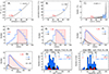 |
Fig. C.1. Effect of inclination. A: Fraction of axes at inclination ϕ < i vs i, assuming random inclinations. The red and blue dots mark two inclinations used in the discussion. B: Same as for A) but vs v sin i, adopting equatorial v = 100 km/s. C: Fraction of v sin i values for equidistant bins d v sin i = 1 km/s. The red and blue numbers give the cumulative contributions of the red and blue shaded area. D: Adopted constant distribution of stars with equatorial veq between 100 and 200 km/s (red shaded rectangle) and v sin i distribution resulting for random inclinations (blue histogram). The two black curves are the distribution in panel C scaled in v for 100 and 200 km/s. The blue histogram is constructed from the integration of all such black curves, it is scaled to the same area as the red histogram. About 30% of the stars from the rectangular red histogram will be observed with v sin i< 100 km/s. E: Same as for D) but separated with an inclination cut i > 30° (blue) and i < 30° (black). F: Same as for E) but adopting a triangular distribution of equatorial v between 50 and 350 km/s (red shaded). G: Same as for F) but allowing for a deviation between iorb and irot with a tolerance of 30° for co-axial rotation (Sect. C.3). The last two panels show the rotational velocity distribution of stars in close SB2 systems with known orbital inclination, without and with inclination correction (middle panel: v sin i, right: v equatorial). |
For randomly oriented rotation axes, the probability of finding an axis inclination ϕ within a cone angle i with the line-of-sight is P(ϕ < i) = 1 − cos (i). This is illustrated in Fig. C.1, panel A. Marked is the case of i = 30° and P = 0.134. This yields the cumulative fraction for v sin i, in other words the fraction of measured vsin(ϕ) cumulated for all inclinations ϕ < i (panel B).
From this we can derive the fraction of v sin i for equidistant narrow bins of 1 km/s (panel C). For example, 13.4% of a sample with intrinsic v = 100 km/s and randomly oriented axes will show v sin i < 50 km/s. Remarkable is also the inclination range i > 60°, where 50% of the sample show v sin i > 87 km/s (i.e. very little affected by inclination).
So far, we have adopted a sample with a fixed intrinsic velocity (veq = 100 km/s). There the histogram peaks at 100 km/s but random inclination produces a declining tail towards smaller v sin i. How will the v sin i distribution appear for a range of veq?
Panel D considers a sample with a constant distribution of the intrinsic velocity veq between 100 and 200 km/s (red shaded); this velocity range is typically observed for vorb. The blue histogram shows the predicted v sin i distribution which will be observed for randomly oriented rotational axes.11 The striking histogram feature is the steep rise from 200 km/s to 100 km/s followed by a steep decline towards smaller v sin i. Compared to panel C with a declining tail towards smaller v sin i, the histogram of panel D appears more symmetric showing two tails. For about 30% of this sample the predicted v sin i lies below 100 km/s.
Panel E assumes a sample with the same veq input distribution as Panel D, but the randomly oriented rotational axes are separated for favourable (i > 30°, blue) and misaligned inclinations (i < 30°, black).
Cases D and E consider an isolated block of input veq, which does not take into account the influence of neighbouring faster or slower veq populations onto the predicted v sin i distribution, for example.
Panel F assumes a triangular input distribution of the intrinsic velocity veq between 50 and 350 km/s (red shaded) seen with random inclinations 0° < i < 90°. Such an input distribution is motivated by the observed triangle-shaped v sin i distribution of SBs. Strikingly, the predicted v sin i distribution (blue, for i > 30°) largely resembles the input distribution, with only a small tail of v sin i below 50 km/s which comprises a fraction of about 10%. The black histogram refers to i < 30°.
Panel G shows the same as Panel F but assuming a mild co-axial rotation, explained in Sect. C.3.
For comparison, the observed v sin i distributions for SB and C dwarfs are depicted in last two panels.
C.2. Inclination of the orbit axis
There are four possibilities for a system to be classified as C:
-
1)
it is intrinsically a single star,
-
2)
it is intrinsically an SB but the distance between primary and companion is too large,
-
3)
it is intrinsically an SB but the mass ratio companion/primary is too small,
-
4)
it is intrinsically an SB but has too a small inclination of the orbit axis.
In cases 2-4, the observed RV variation may be too small so that the system escapes SB detection.
We first discuss the influence of iorb on the SB classification. To detect an SB, iorb must be sufficiently large because otherwise any RV variations (dRV) would be too small to be detectable. If iorb is too small, then the system would be classified as C.
To estimate the inclination threshold at which the transition from an SB to a C likely occurs, we adopt an intrinsic vorb = 100 km/s. For iorb = 15° one obtains sin (iorb) = 26 km/s and a cumulative probability P= 3.5% (Fig. C.1, panel B). To detect an SB, a dRV of ∼25 km/s may be sufficient but requires good luck with the observations. Therefore, we choose a conservative “worst case” threshold iorb = 30°, yielding vorbsin(iorb) = 50 km/s and P≈ 13% (Fig. C.1, panel B).
With this threshold, and assuming randomly oriented orbit axes, the detected SBs comprise (at least) 87% of the entire SB population, and (at most) 13% of the binaries are misaligned and observed (i.e. hidden) as C. This yields a “hiding fraction” hf = 13/87 = 0.15. For a range of 100 km/s < vorb < 200 km/s about 8% of the binaries will appear as a C (black histogram of case E in Fig. C.1).
To compare with observed numbers, our sample contains 130 Cs and 108 detected SB systems (36 SB1, 64 SB2, 8 SB3). Applying the hiding fraction above yields the number of predicted misaligned SBs as 108 ⋅0.15∼16. This comprises only 12% of the Cs (16/130). It rejects the possibility that a significant fraction of the Cs are misaligned SBs (more precisely: are the misaligned counterparts of our detected SB systems).
We conclude that the vast majority of the Cs (likely more than 85%) are either single stars or binaries with small vorb (i.e. with wide orbits or small companion/primary mass ratios). The majority of Cs in our sample must be intrinsically different from the SBs systems. This conclusion is further supported by the different fraction of dwarfs (44% vs 69% in Cs and SBs, respectively, Fig. 11).
C.3. Inclination of the rotation axis
The aim is to quantify the effect of inclination also with respect to the three categories slow/medium/fast rotators.
The samples comprise in total 130 Cs and 176 stars in SB systems. The number of fast rotators in both SBs and Cs (16 and 20 stars, respectively) is small making it unlikely that their inclined counterparts have a significant effect on the statistics of the medium rotators. The number of medium rotators in SBs is 62 stars (13 in SB1, 49 in SB2+SB3) compared to 20 in Cs; when restricting to dwarfs, the numbers are 46 in SBs and 7 in Cs (Fig. 11). Using all stars, the observed fraction of medium rotators is 62/176 = 35% for SBs and 20/130 = 15% for Cs. This yields an excess of medium rotators in SB stars by a factor of 35/15 = 2.3 compared to Cs.
Firstly, we discuss the number of medium rotators and their observed excess for SB stars compared to Cs, assuming that irot is randomly oriented in all stars. For both samples we consider the fraction of intrinsic medium rotators which is hidden (i.e. shifted to slow rotators due to inclination). We adopt the same threshold i = 30° used in the discussion of iorb (Sect. C.2). Applying the hiding fraction hf = 0.15 as above, we obtain, for instance, 9 hidden stars in SBs (62 x 0.15) and 3 hidden stars in Cs (20 x 0.15). A correction for the hidden medium rotators lies in the range below 10%. It would mildly increase the medium rotator excess.
However, it has been widely assumed or speculated that the spin axes of stellar rotation and orbital rotation are roughly aligned (i.e. co-axial). Because the SB systems are preferentially oriented at large iorb > 30°, co-axial rotation implies that irot and v sin i is larger for the detected SB stars than for those Cs, which are misaligned SBs. Then the stars of misaligned SBs are shifted to slow rotating Cs, because sin(i) < 0.5 (e.g. 200 km/s goes to 100 km/s or less). For a rough estimate, we adopt that 16 SBs are misaligned and classified as C (Sect. C.2). We assume as an upper limit that each of them contains two intrinsic medium rotators which appear now as slow rotating Cs. Then the number of true Cs may reduce from 130 to 98 (i.e. by ∼ 25%). A correction will mildly lower the medium rotator excess.
The above estimate assumed that rotation axis and orbit axis are parallel. It did not take into account the possible effect caused by a deviation of rotation axis from the orbit axis. Therefore we refined the estimate, whereby we need some empirical model assumptions. We consider two cases of co-axial rotation:
-
1)
Strict co-axial rotation assumes that rotation axis and orbit axis are parallel, implying irot = iorb.
-
2)
Mild co-axial rotation allows for a deviation δi of rotation axis from the orbit axis by a tolerance up to 30°. (This threshold appears reasonable: the inclination of the earth’s rotation axis against the ecliptic axis is 23°.) To parameterise the deviation distribution, we have chosen a cosine function fdev = cos (3 ⋅ δi) for −30 < δi < 30.
In both cases we assume a triangular input distribution of veq and calculate the predicted v sin i distributions. Panels F and G of Fig. C.1 illustrate the results for strict and mild co-axial rotation, respectively. The blue histograms show the predicted v sin i distribution for the SBs (iorb > 30), the black histograms for the Cs (iorb < 30). The difference between panels F and G is marginal; G predicts slightly more slow rotators. Notably, the blue histograms of F and G appear similar to the observed SB distribution. This suggests that panels F and G describe a realistic case for the SBs. Then the black histograms would quantify how the misaligned SBs may contribute to Cs.
We also compared with literature results on inclination effects. Assuming that the rotation axes are randomly distributed, Ramírez-Agudelo et al. (2013, 2015) deconvolved the observed v sin i distributions with a Bayesian approach and presented an intrinsic rotation distribution of the Cs and the SB2 Primaries in the VFTS, respectively. Instead of the simple triangular input distribution of veq used by us in panels F and G, their adopted input distribution is the sum of a Gaussian and a Gamma distribution. This refined input model has in total (at least) six free parameters (3 for the Gamma distribution and 3 for the Gaussian). If the rotation axis angles are not randomly distributed and our v sin i histograms with about 18 bins (i.e. data points) are noisy, any refinements of the intrinsic rotation distribution compared to our simple triangle estimate should be considered with care. Therefore, the simple triangle estimate is sufficient for our purpose here to estimate the inclination effects (i.e. the shift of medium rotators to slow rotators).
To summarise the theoretical considerations, we have performed a simple estimate with minimal assumptions and by calculating the predicted v sin i distribution from two empirical models, a rectangular and a triangular input distribution of veq. In both cases, we conclude that the medium rotator excess in SBs compared to Cs is real and not caused by inclination effects. Likewise, the predicted fraction of increased rotators which will be shifted by inclination to slow rotators is moderate, less than 30%. We note that fractions of this range are by far too small to significantly reduce the observed excess of medium rotators in SB stars compared to Cs by the factor 2.3, mentioned at the begin of this section.
To compare with real data, our sample contains 53 SB2s with known orbital inclination. Assuming that rotation axis and orbit axis are parallel, we derived the inclination corrected “true” rotational velocities. These and the observed rotational velocities are shown versus the orbital period in the bottom panels of Fig. 16. The sample splits into 28 close SB2s with presumably well-determined veq and 25 wide SB2s with uncertain veq due to uncertain parallelity of spin and orbit axes. The results for the close SB2s are shown in Fig. C.1: The observed and true number counts for slow/medium/fast rotators are 21/30/5 and 4/39/13, respectively. This yields 52 (= 39 + 13) true increased rotators, and 17 (= 21 - 4) observed slow rotators which are shifted by inclination into the slow bin. The shift fraction of 17/52 = 33% appears well consistent with the fraction of 30% predicted above from the rectangular model. The corresponding number counts for the wide SB2s are 32/11/7 and 20/17/13, respectively. This yields 30 true increased rotators and 12 shifted slow rotators, hence a shift fraction of 40%, exceeding the model predictions. The inclination correction of the 25 wide SB2s may be erroneous, and we consider their results with some caution. Notably, the histograms of the true rotational velocities of the close and wide SB2s differ in shape, being rather rectangular and triangular respectively. So far, we can only speculate that the rectangular-triangular difference is not simply a matter of the small number statistics, but has a physical origin. More detailed inclination studies require larger data samples, which is beyond the scope of this paper.
All Tables
All Figures
|
Fig. 1. Statistics of the spectra. Top: Number of spectra per star. The star index is sorted in ascending order of the total number of spectra per star (Ntot, black), and for equal Ntot in ascending order of the number of BESO spectra (red). Bottom: Cumulative fraction of the number of spectra for Cs and SBs, zoomed in to the range 0–30. The dotted lines mark the median; Cs have statistically (about 9/12) fewer spectra than SBs. |
| In the text | |
|
Fig. 2. Mirrored asymmetric line profiles and their Fourier transforms. Example from CPD−58°2611 in the He I 5876 line. Top: Original line profile with an asymmetric blue wing (black dashed), as well as the three types of symmetric line profiles: mirroring the red (v > 0 km/s) and blue (v < 0 km/s) halves of the line profile, and in green the averaged mirrored line profile. Middle: FT amplitude of the original line profile (black dashed), and the mirrored profiles (red, blue, green). Bottom: FT of the original asymmetric profile resembles a smooth chain of data points in the complex plane with non-zero imaginary part. The data point of the first minimum of the FT amplitude is marked in red. |
| In the text | |
|
Fig. 3. One of the worst cases (DT 5) of the effects of disentangling residuals of HD 152219 in He I 4922. Top, two left panels: Single spectra as observed on 2004 May 09 and on 2006 May 06. The two right panels show the average of the two spectra and of all nine spectra used, whereby each component has been shifted to RV = 0 before averaging. The black lines mark Gaussian fits to the profiles, with FWHM and height Aline labelled. Likewise, the peak-to-peak amplitude of the residual wiggles, Ares, is given, determined outside of the velocity range ±3σ of each profile marked by the coloured vertical bars. Averaging reduces the residual wiggles. Bottom: Fourier transform amplitude of the average of all nine spectra, for the primary (left panel), and for the secondary including and excluding residuals (middle and right panel, respectively). The details are explained in Sect. 3.2.3. |
| In the text | |
|
Fig. 4. Distribution of v sin i errors in the helium I lines for single-lined stars (left) and for stars in SB2+SB3 systems (right). The width of the histogram bins is 3%. The details are explained in Sect. 3.2.4. |
| In the text | |
|
Fig. 5. v sin i distribution of different lines. Left for single-lined stars. Right for stars in SB2+SB3 systems, whereby the 25 B-type companions are excluded because their v sin i has been derived solely from He I lines. The legends also list the number of stars with the bestv sin i from O III (green) and He I (red). |
| In the text | |
|
Fig. 6. v sin i distribution derived from O III (green) and He I (red) for single-lined stars (left) and for stars in SB2+SB3 systems (right). Only stars with v sin i measurements in both O III and He I are used. The histogram bin size is 20 km/s. The vertical dotted lines separate slow, medium, and fast rotators. The number of stars in the slow, medium, and fast bins and in total are given, as well as the modes of the distributions. |
| In the text | |
|
Fig. 7. Comparison of v sin i of C and SB1 stars from this work with those measured by Holgado et al. (2022). The values scatter around unity (solid diagonal line). Regarding the C/SB1 classification, the Holgado et al. sources with line profile variation (LPV) are matched with our Cs. Stars with different C/SB1 classifications are marked: we find more slow SB1s (red) and Holgado et al. find more fast SB1s (blue). |
| In the text | |
|
Fig. 8. Comparison of v sin i of disentangled SB2 and SB3 components from this work with collected values in the literature (Table D.2). The values scatter around unity (solid diagonal line), within ∼30% (dashed lines). The black arrows are upper limits. |
| In the text | |
|
Fig. 9. Dependence of v sin i of single stars (C) on spectral type and luminosity class. Among giants and dwarfs, respectively, the early-type stars (blue) show a ∼10 km/s faster v_peak than the late-type stars (red). Likewise, the v_peak of giants is faster than that of dwarfs. |
| In the text | |
|
Fig. 10. Rotational period of single stars. Prot = 2πR*/v. The vertical dotted line at Prot = 5 d corresponds to v ≈ 100 km/s for an O7.5 V star. Dwarfs exhibit a clear short-period peak. The median period is given for the bulk of stars with long periods > 5 d. |
| In the text | |
|
Fig. 11. v sin i distribution of the spectroscopic binary types. The 140 stars in SB2+SB3 systems are 72 primaries, 62 secondaries, and 6 tertiaries. v_peak gives the mode and standard deviation of the v sin i distributions for LC I+II (red) and IV+V (blue); LC III has too few data points. |
| In the text | |
|
Fig. 12. Calibration mass and semi-major axis vs. orbital period. Left for SB1 and right for SB2. Top: Mass, the horizontal line marks the median mass. Bottom: Semi-major axis, the solid line marks a least-squares fit to the data (logarithmic, with the fit equation labelled). The vertical and horizontal lines are for guidance (dashed and dotted). Bottom right: Blue and red distinguish the mass ratio, the coloured numbers give the number of SB2s in the Porb bins separated by Porb = 10, 100, 1000. |
| In the text | |
|
Fig. 13. v sin i vs. orbital period. Top: For SB1 (left) and SB2 (right), each primary–secondary pair is connected with a vertical dotted line. Bottom: SB2 primaries and secondaries plotted separately; for the secondaries the black encircled symbols mark B-type companions. |
| In the text | |
|
Fig. 14. Histograms of v sin i for close and wide SB2s separated by Porb = 10 d, from left to right for primaries, secondaries, and the entire samples. Top row: Close SB2s. Bottom row: Wide SB2s. |
| In the text | |
|
Fig. 15. Ratio of literature to calibration radius Rlit/R* of the stars vs. orbital period for the 19 SB2s where a literature radius is available (Table D.2). For each SB2 the vertical dotted line connects the primary and secondary. Unity is marked by the horizontal solid line, and the average and its standard deviation by the horizontal long-dashed and dash-dotted lines, respectively. The blue three-dot-dashed line is an ordinary least-squares fit (log Y vs. log X) of the primary data. |
| In the text | |
|
Fig. 16. Dependence of rotational properties on the orbital period. Top: Rotational period vs. orbital period for SB1s (left) and SB2s (right). The y-axis of Fig. 16 is inverted in order to preserve that faster (slower) rotating stars are plotted up (down). The vertical long-dashed line separates close and wide binaries. The solid diagonal line labelled ‘sync’ marks equal periods, as required for synchonised rotation, whereby an inclination i = 30° of the rotational axis shifts the data points from this line by a factor of 1/sin(30°) = 2 to the dotted inclination line labelled ‘i = 30’. The two SB2s below the dotted inclination line indeed have known iorb < 20° (HD 048099 and HD 167771). For SB2s, the components are connected with a vertical dotted line; for most wide binaries at Porb > 10 d, Prot differs strongly between the components but the difference reduces and disappears for close binaries. Middle left: Ratio of Prot of the binary components vs. Porb; the horizontal lines mark the median in each Porb range. Middle right: Prot vs. Porb for those 53 SB2s with known inclination of the orbital axis iorb; Prot is corrected for inclination assuming parallel orbital and rotational axes. The solid and dotted diagonal lines mark the synchronisation range with a width of 30% and a factor of 2, respectively. The green triangle marks the range above the sync line discussed in the text. Bottom left: v sin i vs. Porb for the 53 SB2s with known iorb. Bottom right: veq vs. Porb after correction for the inclination. |
| In the text | |
|
Fig. 17. Mass ratio vs. orbital period. Blue and red indicate whether the primary or secondary is the faster component (measured by v sin i). Among wide binaries, the large symbols mark those pairs where at least one component is a medium or fast rotator (6 blue and 17 red pairs; see Sect. 5.3.1). |
| In the text | |
|
Fig. 18. Rotational asymmetry between primaries and secondaries, for all wide binaries (left column), and for a subset where at least one component is an increased rotator (right column). Medium wide and very wide binaries are coloured in blue and red, respectively. Top: Ratio of the rotation periods P/S vs. mass ratio; the size of the circles indicates the orbital period, i.e. component separation, on a logarithmic scale. Bottom: Histograms. |
| In the text | |
|
Fig. 19. Stars are born with different spins. Before the main sequence phase, fragmented cloud cores merged and the resulting stars feature slow (red) and increased (blue) spin. |
| In the text | |
|
Fig. 20. Hierarchical triple system. The two massive stars form a wide SB2, consisting of one slow and one increased rotator (red and blue, respectively). Left: Increased rotator itself is a close SB1 with a hidden lower mass companion, the tertiary star (green). The tertiary may produce strong radial velocity variations. Right: Increased rotator has two hidden lower mass components (green) orbiting such that they balance out strong radial velocity variations of the high-mass star. |
| In the text | |
|
Fig. 21. Fly-by in an unstable triple system. The binary system of two massive slow rotators (red) captured a lower mass star (green) that interacted in a close fly-by with one of the massive stars before being ejected. The spin of the closely flown-by star may be increased a bit (blue). |
| In the text | |
|
Fig. 22. Swallowing of a low-mass star in a triple system: A low-mass star (green) initially moves in the gravitational field of a wide high-mass binary with two slow rotators (red). When the orbit of the low-mass star is disturbed, it spirals on to one of the high-mass components. The resulting post-merger star has an increased mass and spin (blue). |
| In the text | |
|
Fig. 23. Fragmentation of a cloud or disk into three cores of different size and mass. They form three stars (or proto-stars) of high, medium, and low mass, respectively. During subsequent evolution, the stars interact and merge. |
| In the text | |
|
Fig. A.1. Examples of disentangling types (DT) for SB2s (DT 1-6) and SB3s (DT 7-8). Details are described in Sect. A. Radial velocities “v” are as observed and not corrected for systemic velocities. |
| In the text | |
|
Fig. B.1. Effect of the emission of an isotropic slow wind on the line profile (top) and its Fourier transform (FT, bottom), for two rotation speeds v sin i = 0 km/s (“null rotator” left) and v sin i = 100 km/s (“mid rotator” right). Top: The blue solid line shows (1) the rotating star, a rotationally broadened line profile convolved with Lorentzian, vrot = 50 km/s, FWHM vturb = 50 km/s. The red solid line shows (2) an isotropic slow wind halo with vwind = 50 km/s and dispersion ≈ 20 km/s (total FWHM ≈ 65 km/s). The wind strength is 5% of the stellar equivalent width. The dash-dotted black line shows the combined profile of star and wind (sum of (1) and (2)). We note that the combined profile has a rounder (i.e. more boxy) shape than the pure stellar profile. Bottom: FT amplitude of the rotating star (blue), of the wind halo (red), and of the combined profile (star and wind, black). |
| In the text | |
|
Fig. C.1. Effect of inclination. A: Fraction of axes at inclination ϕ < i vs i, assuming random inclinations. The red and blue dots mark two inclinations used in the discussion. B: Same as for A) but vs v sin i, adopting equatorial v = 100 km/s. C: Fraction of v sin i values for equidistant bins d v sin i = 1 km/s. The red and blue numbers give the cumulative contributions of the red and blue shaded area. D: Adopted constant distribution of stars with equatorial veq between 100 and 200 km/s (red shaded rectangle) and v sin i distribution resulting for random inclinations (blue histogram). The two black curves are the distribution in panel C scaled in v for 100 and 200 km/s. The blue histogram is constructed from the integration of all such black curves, it is scaled to the same area as the red histogram. About 30% of the stars from the rectangular red histogram will be observed with v sin i< 100 km/s. E: Same as for D) but separated with an inclination cut i > 30° (blue) and i < 30° (black). F: Same as for E) but adopting a triangular distribution of equatorial v between 50 and 350 km/s (red shaded). G: Same as for F) but allowing for a deviation between iorb and irot with a tolerance of 30° for co-axial rotation (Sect. C.3). The last two panels show the rotational velocity distribution of stars in close SB2 systems with known orbital inclination, without and with inclination correction (middle panel: v sin i, right: v equatorial). |
| In the text | |
Current usage metrics show cumulative count of Article Views (full-text article views including HTML views, PDF and ePub downloads, according to the available data) and Abstracts Views on Vision4Press platform.
Data correspond to usage on the plateform after 2015. The current usage metrics is available 48-96 hours after online publication and is updated daily on week days.
Initial download of the metrics may take a while.