| Issue |
A&A
Volume 690, October 2024
|
|
|---|---|---|
| Article Number | A124 | |
| Number of page(s) | 10 | |
| Section | Stellar structure and evolution | |
| DOI | https://doi.org/10.1051/0004-6361/202451405 | |
| Published online | 03 October 2024 | |
Detection of faint secondary companions in spectroscopic binaries
1
Instituto de Ciencias Astronómicas, de la Tierra y del Espacio, Casilla de Correo 49, 5400 San Juan, Argentina
2
Observatorio Astronómico Félix Aguilar, Universidad Nacional de San Juan, Av. Benavidez Oeste, 8175 San Juan, Argentina
Received:
6
July 2024
Accepted:
31
July 2024
Abstract
Context. Most known spectroscopic binaries are detected through the variation in the radial velocity of the primary star, while the spectral features of the secondary companion remain hidden in the noise.
Aims. We present a novel technique for the spectroscopic detection of low-luminosity secondary companions of binary stars. The main goal is to estimate the mass ratio even when the radial velocity of the secondary cannot be measured in individual spectra.
Methods. The method aims to bring together all the spectral information of the secondary component into one single feature. In a first step, a spectral disentangling technique is used in an automatic way for a grid of possible values of the mass ratio. Then, the resulting series of secondary component spectra are compared with a grid of synthetic templates with a technique inspired by spectral cross-correlations. By optimizing a function indicative of the significance of the secondary detection, the mass ratio and an estimate of effective temperature are derived.
Results. We apply our method to different types of objects and observational datasets: three single-lined spectroscopic binaries in the open cluster Blanco 1 observed at mid-spectral resolution, an early-type binary in the open cluster NGC 2362, and PX Vir, an F-type binary observed at high resolution for which the secondary companion had been detected in the infrared but not in the optical spectral range. It is shown that from standard-quality spectral datasets it is possible to detect the secondary star in systems in which the secondary contributes less than 0.5–1.0% of the total flux.
Key words: methods: data analysis / techniques: spectroscopic / binaries: spectroscopic
Corresponding authors; This email address is being protected from spambots. You need JavaScript enabled to view it. , This email address is being protected from spambots. You need JavaScript enabled to view it. .
© The Authors 2024
 Open Access article, published by EDP Sciences, under the terms of the Creative Commons Attribution License (https://creativecommons.org/licenses/by/4.0), which permits unrestricted use, distribution, and reproduction in any medium, provided the original work is properly cited.
This article is published in open access under the Subscribe to Open model. This email address is being protected from spambots. You need JavaScript enabled to view it. to support open access publication.
1. Introduction
Knowledge of the frequency and properties of binary stars has a key role in stellar astrophysics. Besides their known and exploited role as tools for the determination of stellar physical parameters, the eventual interaction between components gives place to a variety of exotic stellar objects, and the multiplicity frequency in different mass ranges and environments offers constraints on star formation theories. In the statistical analysis of spectroscopic binaries, an awkward fact is that most of them are single-lined binaries (SB1s), which means that in most cases nothing is known about the secondary component, other than a possible upper mass limit provided by the mass function. As an illustration, among all binaries with orbits in the SB9 Catalogue of spectroscopic binaries (Pourbaix et al. 2004), 75% are SB1s. This causes a severe problem for the statistical study of mass ratios, for example. In fact, assuming a random orientation of the orbit in the space for SB1s, the derived mass ratio distribution for SB1s is completely different than the observed q-distribution for SB2s, due to selection effects (Hogeveen 1992). The fact that 80% of the cataloged double-lined binaries (SB2s) have a mass ratio larger than 0.5 is largely due to the difficulty of detecting low-mass companions. This issue is related to the well-known fact that luminosity (or optical flux) scales as a large (∼3) power of stellar mass along the main sequence, so that the flux contribution of a secondary is below 5% and usually below 1% in binaries whose components differ by a factor of 2–3 in mass. This is illustrated in Fig. 1, in which the expected V-band flux contribution of the secondary is plotted as a function of the mass ratio for synthetic binaries of two different masses and two evolutionary stages. PARSEC stellar models (Bressan et al. 2012; Nguyen et al. 2022) have been used in these calculations.
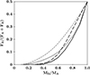 |
Fig. 1. Flux contribution of the secondary companion as a function of binary mass ratio. Four models are shown: a primary of 10 M⊙ (thin lines) and 2 M⊙ (thick lines) for ages close to the primary terminal-age main-sequence (solid lines) and about half the main-sequence lifetime (dashed). |
Considering that this is just a problem of contrast and signal level – at a high enough signal-to-noise ratio (S/N), all SB1s eventually become SB2s – we propose in this paper a strategy to enhance, as much as statistically possible, the signal corresponding to the faint spectral component. The emphasis is put on measuring the mass ratio. Increasing the number of binaries for which the secondary is detected implies not only improving the statistics but, most importantly, extending the knowledge of the mass ratio distribution to lower values.
In this work, we outline the fundamentals of our technique and demonstrate its applicability to different types of binaries. In a separate work (Martínez & González, Paper II, in prep.), we present the application through a PYTHON repository and address the study of a sample of late-type stars aimed at searching for low mass companions.
The paper is organized as follows. Sections 2 and 3 describe the proposed method and discuss the problem of detection of faint secondaries. Sections 4, 5, and 6 show application cases for different types of objects. Finally, a general discussion is given in Sect. 7.
2. The method
The underlying concept of the method is to maximize the signal from the secondary star by combining all their spectral lines in all the observed spectra into one single measurable feature. The two main steps are, therefore, a) the combination of all available spectra to produce a master spectrum of the secondary, and b) the combination of all the spectral information in that master spectrum into one single feature. The goal of the first stage is to get the average spectrum of each of the stellar components. Since the line sets of the two components move in wavelength, some spectral disentangling technique has to be applied.
The procedure for the calculation of the spectrum of the secondary component is as follows. Using a set of N observed spectra of the object, an SB1 binary, the radial velocity (RV) of the primary is measured and the resulting RV curve is modeled by any standard method. Since the center-of-mass RV, γ, is known from the orbit fit, at this point the RV of the secondary (VB) could be calculated for each observation from the RV of the primary (VA) if the mass ratio q ≡ MB/MA was known, using the expression
 (1)
(1)
q being unknown, a grid of possible values of q is defined and these calculations are performed for each q. Once the RVs of both components are calculated, all the observed spectra are combined using the spectrum calculation routine of the disentangling method by González & Levato (2006) to reconstruct the separate mean spectra of the two stellar components. This is possible because for the reconstruction of the secondary spectrum, it is not necessary for the observed spectrum to have any visible spectral lines of the secondary, but to know the RV of both components for each observation.
The S/N in the master secondary spectrum, Bq, is about  times higher than in the individual observations; however, this might not be sufficient to distinguish their lines above the noise. The second step is, therefore, to gather all the spectral information in one single feature. A simple and widely used technique that allows one to do this is cross-correlation.
It can be shown that the S/N of the peak of the cross-correlation function scales approximately as the square root of the number of spectral lines, as in the case of averaging line profiles. This is what makes it possible to measure the RV of late-type stars in very low-S/N spectra. Since we are trying to detect low-luminosity companions, in most cases secondaries will be late-type main-sequence stars whose spectra typically have hundreds of useful lines in the optical range.
We note that the reconstructed spectrum of the secondary star, Bq, has, by definition, zero RV. Therefore, the cross-correlation function of this spectrum against a synthetic template, 𝒯, with the appropriate spectral morphology would give a peak centered at zero. The height of this peak is then taken as a proxy of the detection significance. Since the spectral morphology of the secondary component is unknown, a grid of synthetic templates for a range of effective temperatures is used. For the application examples of the present paper, these templates were taken from the spectral library of Coelho et al. (2005) for log g = 4.0 and solar abundances. In this way, the binary mass ratio and the secondary star temperature can be determined by maximizing the two-variable function, ℱ(q, Teff, B), which we shall call here the secondary significance function (SSF).
It is important to note that to calculate the SSF it is not necessary to calculate the whole cross-correlation function for each combination of secondary star spectrum and template, but only its value at RV = 0. In other words, the SSF is simply the normalized integral of the product of both spectra:
 (2)
(2)
which greatly reduces the computation times. In the classical definition of the cross-correlation function (aimed at deriving RVs), the norms that appear in the denominator, |X| = [∫|X|2dλ]1/2, are constant factors that ensure that the function is higher the more alike the spectral morphology of the object and the template spectra are, independently of the global intensity of the lines. In our case, the secondary line intensities are expected to be higher for the correct value of q. To take advantage of this fact, it is convenient not to divide by the norm of Bq. In practice, our default strategy is to use a constant value, |Bmax|, corresponding to the Bq for which the norm is maximum. The adoption of this particular value responds to the fact that it will roughly correspond to the correct value of q.
The integrals in Eq. (2) cover in principle the whole spectrum, but in practice they can be restricted to some wavelength ranges to avoid noisy regions, instrumental artifacts, telluric lines, etc. Optimal weights as a function of wavelength can also be calculated from the template morphology and the noise level. In the present paper, a simple weighting scheme was applied, assuming that the original spectra are in the shot-noise-limited regime, in which the noise level scales as the square root of the flux intensity. In this approach, a smooth spectral flux distribution (a “continuum” in a non-flux calibrated observed spectrum) represents reasonably well the appropriate weight of each wavelength region. In practice, this was implemented simply by using non-normalized observed spectra. Instead of normalizing the object spectra, template spectra were multiplied by the mean continuum of the observed spectra to make them morphologically consistent. Before cross-correlations, the spectra were rectified by subtracting a fitted continuum. This strategy is in fact the usual procedure in cross-correlations for RV measurements.
We note that our primary aim is neither to obtain a useful spectrum of the secondary star nor to measure its RV in individual spectra. The final outcome of this method is the value of the mass ratio (which gathers information about the amplitude of the secondary RV curve) and the secondary temperature (a parameter roughly describing the spectral morphology of the secondary star).
An additional parameter that can be estimated is the flux ratio or, equivalently, the flux contribution of the secondary to the total flux. This can be calculated by fitting the best scaling factor between the synthetic template and the secondary spectrum, Bq. We assume that the spectral morphology of the secondary spectrum, B, can be fitted by the template, 𝒯, scaled by a factor, α, plus a possible zero-level difference: B = α𝒯 + Z, where α and Z might vary slowly with wavelength. We applied two strategies to estimate the factor, α. In the first one, the best value for the scale factor is calculated through the expression
 (3)
(3)
where ⟨⟩ symbolized a running average over a small spectral window. We implemented these calculations using box smoothing. However, since the uncertainty of the obtained value at a certain wavelength depends on the intensity of lines, the similitude of the spectral morphology, and the noise level in that spectral region, a second α spectrum is produced by applying a running weighted average over the α spectrum.
The second strategy is to directly calculate the square difference, |B − α𝒯 − Z)|2, for a grid of α values to numerically find the one that minimizes the residuals. In the examples shown in the following sections, we applied this latter strategy in small spectral windows (80–300 Å) to account for slow variations in α along the spectrum. In any case, the scale factor calculated through these techniques has to be considered only as an estimate, since eventual morphological differences between the secondary spectrum and the adopted template can easily cause errors of 10–20% in α, as will be discussed.
As an illustration of the secondary companion detection, Fig. 2 shows the S/N enhancement in an artificial example corresponding to what might be a typical case. We built a synthetic binary star formed by an A8 V primary with 1.7 M⊙ and a K7 V secondary with 0.64 M⊙. We adopted temperatures of 7600 K and 4000 K and radii for main-sequence stars of those masses. The mass ratio is q = 0.376 and the resulting flux ratio is about 0.0018 at λ4500 and 0.0046 at λ5700 (Fig. 2a). In other words, the secondary is about 6 mag fainter than the primary. With an orbital period of P = 500 d, the observed RV curve in this binary has a semi-amplitude of KA = 9.7 km s-1. We modeled an observation sample consisting of 20 binary spectra of S/N ∼ 80, randomly distributed in orbital phases. The spectra cover the spectral range 5300–5800 Å with a resolving power of 50 000 and a sampling of 0.015 Å.
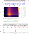 |
Fig. 2. Detection plots for the secondary companion in a synthetic example. a) One of the 20 artificial binary spectra of the demonstration example. The “observed” composite spectrum (black) is compared with component synthetic spectra (primary in blue, secondary in red) to show the intensity of the secondary lines. The lower spectra have been multiplied by 50 for better visibility. Arbitrary vertical shifts have been applied. b) SSF in the q − Teff plane. Green lines mark the position of the maximum and next to both axes the corresponding cross-sections defining the best solution (Teff = 4000 K, q = 0.37) are shown. c) Reconstructed secondary spectrum (black) compared with a synthetic noise-free spectrum of 4000 K (red). d) Cross-correlation function corresponding to the adopted solution. |
The upper panel of Fig. 2 shows in black one of the composite input spectra and below in the same panel, the input noise-free spectra of the components to show the size of secondary lines in the spectrum. A rough estimation of the original S/N of the secondary lines and the final S/N of the detection peak can be done as follows. In a late-type star, which is the typical case for faint secondaries, the depth of typical metallic lines may be on the order of half the continuum level. Therefore, in our synthetic binary, the effective S/N of secondary features (line height over RMS of the spectrum noise) is at λ5700 about 80 × 0.0046 × 0.5 ≈ 0.18. In other words, the spectral lines are five times smaller than the sigma of the spectrum noise, so they are completely masked by the noise.
After spectral disentangling, the effective S/N is increased by a factor of  , reaching S/N ≈ 0.82 (Fig. 2c). The spectral morphology is not apparent, but the downward peaks do not seem to be completely random but instead to have a positive correlation with the expected position of spectral lines. Finally, the cross-correlation function shows a peak ∼27 times higher than the noise, resulting in a very clear detection of a companion ∼200 times fainter than the primary, using observational data of modest S/N. The comparison of the peak height and the noise in the cross-correlation function is taken as the S/N of the detection. We assume here that the subsidiary lobes appearing in the correlation function at nonzero velocities due to the random match between object and template lines are negligible compared to the noise. This is valid since we are dealing with high noise levels and the subsidiary peaks are comparatively small in stars with many spectral lines. Anyway, the presence of a subsidiary peaks has no impact on the calculation of the SSF.
In brief, the calculations of the proposed method are done in practice as follows:
-
The RV of the primary is measured by cross-correlations against an appropriate template.
-
The RV curve is fitted to get the center-of-mass velocity, γ.
-
For each mass ratio in a grid, the RV of the secondary component at each observation time is computed and the secondary spectrum is reconstructed through spectral disentangling.
-
The SSF, ℱ(q, Teff, B), is calculated using Eq. (2).
-
The maximum of the SSF is located, determining the values of q and Teff, B.
-
The secondary-star scaling-factor, α, is calculated using Eq. (3).
-
From the cross-correlation function corresponding to the adopted q and Teff, B, the effective S/N of the detection is calculated.
More technical details and the implementation of the method in a PYTHON repository (open source) are described in the companion paper by Martínez & González (Paper II, in prep.).
3. The fuzzy distinction between SB1s and SB2s
As was already suggested in the introduction, the classification SB1 or SB2 does not apply to a binary star as an astronomical object, but to a given spectroscopic observational dataset of a given binary. In fact, the observation of the secondary lines in the spectrum depends on the wavelength range observed, the spectral resolution, the S/N, and even on the data analysis technique, which is the aspect we want to emphasize here.
As an illustration, Fig. 3 shows the transition between the SB2 and the SB1 domains for different object and observational data properties. The ordinate axis describes the flux contrast between the components, which is the key object property for this problem. As a proxy of the quality of the observations, the S/N of a typically observed spectrum is plotted in the abscissa axis. The curves have been calculated for a data sample of 30 spectra of a binary with a late-type secondary star. Specifically, we assumed that the secondary star is a sharp-lined FG-type star whose spectrum has 200 lines with intrinsic intensity of about half of the continuum level. We defined as detectable a feature with an effective S/N (feature intensity over noise) of 10. Above the black line, individual lines of the secondary star can be identified in an individual observation. For example, for a binary with a secondary star with a flux contribution of 20%, observed at S/N = 100, the effective S/N of the secondary star lines is 0.5 × 0.2 × 100 = 10. This line would be the classical boundary between SB1s and SB2s.
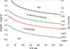 |
Fig. 3. Frontier between SB1s and SB2s. In the upper region (labeled SB2), the spectral lines of the secondary are visible in individual spectra. Between the black and the green curves, the spectral lines of the secondary are not distinguishable in individual spectra but they are clearly seen in the reconstructed spectrum of the secondary, in which the S/N is increased by a factor equal to the square root of the number of observations. Above the red line, the peak of the cross-correlation function is high enough to measure RV in individual spectra. The region labeled with “q measurable” corresponds to configurations in which it is not possible to measure RVs for the secondary star nor to study the spectral morphology of the spectrum, but still it is possible with our technique to calculate the mass ratio. |
The method proposed in this paper attempts to combine N observations and m spectral lines in one feature. With this strategy, it is possible to calculate the mass ratio in all systems above the blue line in the figure. We have assumed here an observational dataset of 30 spectra. Our observations of the stars Blanco 1-W86, Blanco 1-61, and NGC 2362-46, which will be described in Sect. 4, are in this regime. Below the blue line in the figure, the studied binary remains as SB1 unless a larger number of spectra are obtained. An example is the case of the star Blanco 1-W57 shown in Sect. 4.
In the in-between region, there are cases in which the secondary lines are below the noise level in individual spectra but, when applying our program, the reconstructed spectrum of the secondary has a high-enough S/N for its spectral morphology to be analyzed (above the green line in the figure). In some other cases, the secondary lines are below the noise level but the velocity can be measured in individual spectra using cross-correlations. The green, red, and blue lines differ from the black line by a factor of  ,
,  , and
, and  , respectively. An example of this intermediate regime is shown in Sect. 6, in which we analyze HARPS data of the star PX Vir, for which we were able to recover the secondary star spectrum.
4. Application to three binary stars in the open cluster Blanco 1
In a spectroscopic survey of the bright stars in Blanco 1, González & Levato (2009) detected several SB1s. Among them, W57 (CD-30 19801), W61 (HD 225111), and W86 (HD 225264) are the three with the best RV curves; that is, with smaller errors and good phase coverage (see Fig. 1 in that paper). The spectroscopic data used in that work are suitable for testing our technique for the secondary detection: the dataset for each star consists of 15–30 spectra with a high-enough resolving power (R ∼ 13 000) and good spectral coverage (about 4000–6000 Å) but modest S/N (∼50–100), while the secondary stars are expected to be late-type stars well below the magnitude limit of individual observations with that instrument. In our analysis, we added, for the three binaries, a few more spectra taken with the same instrument at a later date. The results for these three binaries are summarized in Table 1 and Figures 4 and 5.
Parameters derived for the three binaries analyzed in Blanco 1.
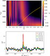 |
Fig. 4. Detection plots for star W57. Top: SSF in the q − Teff plane. The vertical green line marks the lower limit of q according to the spectroscopic mass function and an estimated primary mass of 1.4 M⊙. The yellow line shows the temperature for each possible value of the secondary mass, assuming it is a main-sequence star of the age of the cluster. Bottom: Cross-correlation function of the reconstructed secondary spectrum for several experiments adding artificial secondaries to the observed spectra. The inset shows the contribution of the secondary star to the total flux. |
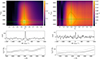 |
Fig. 5. Detection plots for the secondary companion of the binary W61 (left) and w86 (right). From top to bottom: Secondary detection function in the q − Teff, B plane, cross-correlation function for the best B spectrum, and estimated flux contribution of the secondary star. |
The highest signal of the secondary star was found for the system W61, whose results are shown in Fig. 5. The upper panel of this figure shows the value of the SSF in the q − Teff plane. The red contour line corresponds to a level equal to the maximum minus the RMS of the noise of the cross-correlation function, and is plotted as indicative of the uncertainty in the position of the maximum. The middle panel shows the cross-correlation function of the best secondary spectrum (corresponding to q = 0.48 and Teff = 4600 K) against a synthetic template (middle panel), while the lower panel shows the secondary spectrum scale-factor; that is, the flux contribution of the secondary companion. The S/N of the cross-correlation peak is about 18. The flux contribution of the secondary is close to 1% at 5500 Å and about half of that in the blue part of the spectrum. Thus, the secondary would be about 5 mag fainter than the primary in the V band. The detection of the secondary is also clear in the case of W86, although with a lower significance (S/N ∼ 6). The flux contribution of the secondary would be lower than 0.6% in the observed spectral range, being less than 0.2% below 5400 Å.
Finally, in the case of W57 we found no signal larger than 3 σ (Fig. 4). In order to put an upper limit on the secondary flux, we injected secondary features in our observational dataset and performed detection experiments. Specifically, for eight values of q in the range of 0.25–0.50 we calculated the RV of the secondary star and estimated its temperature, assuming it is a normal main-sequence star. Then, we scaled a synthetic template of that temperature according to the expected flux ratio and added the spectrum to each observed spectrum previously shifted according to the RV of the corresponding orbital phase. Finally, we applied our program finding the cross-correlation functions shown in the lower panel of Fig. 4. Three of the eight models have been omitted in the figure for clarity. The black line (0.0%) corresponds to the original observational data. According to these experiments, in our observational dataset we should be able to detect the secondary star at a level of 5σ if the flux ratio is larger than 0.3%, which corresponds to q > 0.37, assuming the secondary is a main-sequence star. We therefore conclude that if the secondary is a normal main-sequence star then the binary mass ratio is in the range of 0.30–0.37. The secondary mass would be an early-M type star with 0.42–0.52 M⊙.
A somewhat higher mass would be possible if its spectral lines were broadened by stellar rotation, but a high rotation is not expected, considering the tidal forces acting in such a short-period binary. The expected value of the projected rotational velocity, vB sin i, can be derived from the spectroscopic orbit if the primary mass is estimated from the cluster color-magnitude diagram and the radius of the secondary star RB is assigned interpolating its mass in the same isochrone. The rotational axis being perpendicular to the orbital plane, the projected rotational velocity of the secondary is
 (4)
(4)
If the mass ratio and the primary mass are known, the factor, sin i, can be obtained from the expression for the RV curve amplitude:
 (5)
(5)
Combining Eqs. (4) and (5), and using the Kepler equation to replace the major semiaxis, the projected rotational velocity can be written as
 (6)
(6)
where the ratio of rotational to orbital periods, Prot/P, is a function of the eccentricity (see Eq. 42 in Hut 1981). For star W57, we obtained v sin i ≈ 9 km s−1, so rotational broadening would not be the cause of the negative result in this case. We mention that the expected rotational velocity of the secondary star is also low for the binaries W61 (12 km s−1) and W86 (10 km s−1), although the latter might not be synchronized, given its eccentricity.
To illustrate the benefits of this technique, Fig. 6 shows the color-magnitude diagram of the cluster, with the location of the companions of the three spectroscopic binaries. The photometric data were taken from the Gaia DR3 catalogue (Gaia Collaboration 2023). The gray points in the figure are probable cluster members selected on the bases of parallax and proper motion. For star W57, two values are plotted for the secondary companion, corresponding to the lower limit imposed by the mass function and the upper limit derived from the non-detection of the secondary spectrum. The horizontal gray line marks the limiting magnitude of the spectrograph for S/N = 100 in a 1-hour exposure.
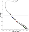 |
Fig. 6. Color-magnitude of the open cluster Blanco 1 in the Gaia photometric system. Squares (triangles) mark the location of the primary (secondary) components of the three studied binaries: w57 (green), w61 (red), and w86 (blue). The gray line marks the magnitude limit of the instrument for a spectrum of S/N = 100 in a 1-hour exposure. |
5. NGC 2362-46, an example of an early-type binary
In the previous section, we showed the search for secondaries in three binaries with A-F type primaries. We show here an example of an early B-type binary observed with the same instrument. HD 57192 is a B2 V (Houk 1982) binary star that is one of the brightest objects in the young open cluster NGC 2362. The spectra show only the lines of the primary, mostly of He I, with small velocity variations (Fig. 7). According to the RV curve (Fig. 8), the mass function is 0.037 M⊙.
 |
Fig. 7. Region of CASLEO spectra of the binary NGC 2362-46 showing He I lines at λλ4387, 4438, 4471 and the Mg II line at λ4481. The spectra are ordered by phase and shifted vertically for better visibility. Note that the RV amplitude is significantly smaller than the width of spectral lines. |
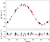 |
Fig. 8. RV curve of NGC 2362-46. The lower panel shows the residuals of the orbital fit. |
Interestingly, this spectroscopic binary is eclipsing (MX CMa, van Leeuwen 2007) and has a visual companion 6 mag fainter at 4.8 arcsec (IDS 07151-2446 B), so it is probably a triple system. The flux contribution of the third companion is not expected to be detected in our analysis or to hamper the detection of the secondary spectroscopic companion, since the spectral lines of the visual companion are expected to be fixed.
The results of the secondary detection are shown in Table 2 and Fig. 9. The secondary is clearly identifiable in the mass ratio temperature diagram, although the S/N is quite low. The mass ratio is only 0.2 and the secondary flux contribution about 0.2%. The primary mass estimated from the spectral type is about 10 M⊙ (Straizys & Kuriliene 1981), although the star position in the color-magnitude diagram suggests a larger primary mass of about 15 M⊙, corresponding to a star of luminosity class III. The secondary star would be an A-type star very close to the zero-age main-sequence, since in this very young cluster (∼5 Myr, Moitinho et al. 2001; Dahm 2005) stars with masses lower than about 2 M⊙ are expected to be pre-main-sequence objects.
Parameters of the binary NGC 2362-46.
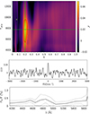 |
Fig. 9. Detection plots for the secondary companion of the binary NGC 2362-46. |
The short period and low eccentricity of this binary suggest that it is tidally locked. Assuming a radius close to 1.9 R⊙, corresponding to the age of the isochrone that fits the Gaia color-magnitude diagram (log τ = 6.8), the projected rotational velocity would be v sin i ≈ 29 km s−1, barely detectable at our spectral resolution. Therefore, even in this short-period binary the rotational broadening of the secondary star does not degrade the cross-correlation peak significantly.
The eclipsing character of this object offers an interesting opportunity to derive absolute stellar parameters that can be used to discuss its connection with the cluster NGC 2362. However, this exceeds the purpose of the present work and will be postponed to a more specific study.
6. A high-quality dataset of a late-type binary: Revealing the secondary spectrum in PX Vir
As a last example, we show a quite different case: a long period, low-RV amplitude, pre-main-sequence binary, observed at high resolution and high S/N using HARPS. In this section, we show that in data samples with a higher S/N (or a larger number of spectra), it is possible not only to measure the mass ratio, but also to reconstruct the spectrum of the secondary with an S/N high enough to study in detail the spectral morphology of the secondary.
Another interesting point in this example is that the masses of the stars have been estimated from interferometric measurements and infrared spectroscopy. In a conference proceeding paper, Cusano et al. (2009) presented preliminary results of a spectroscopic-interferometric study based on HARPS, CRIRES, and AMBER observations. Using HARPS, they obtained the RV curve for the primary star but they were unable to detect the secondary in those optical spectra. However, in infrared spectra obtained with CRIRES they did detect spectral lines from the secondary and estimated the binary mass ratio to be 0.57 ± 0.05. Furthermore, in the same work, they report interferometric observations with AMBER, which allowed them to get the orbital inclination and then the absolute masses, obtaining MA = 0.88 ± 0.13 M⊙ and MB = 0.50 ± 0.07 M⊙. The uncertainties reported by Cusano et al. are most likely underestimated, as was convincingly pointed out by Griffin (2013). Unfortunately, after the publication of those preliminary results, Cusano et al. never published a more detailed work that included their measurements and further data analysis details. Around the same time, Griffin (2010) published a high-quality RV curve obtained with the Cambridge Coravel. These velocities are entirely consistent with HARPS velocities apart from small zero-point adjustments. The joint fitting of both datasets gives P = 216.48 ± 0.02 d, KA = 12.91 ± 0.02 km s−1, e = 0.256 ± 0.002, and ω = 295.6 ± 0.3 deg. In these calculations, we used our own RV measurements on HARPS spectra, but indistinguishable results are obtained with Trifonov et al. (2020)’s velocities.
While our paper was in preparation, Wang et al. (2023) published an astrometric-spectroscopic orbital analysis obtaining the masses MA = 0.74 ± 0.06 M⊙ and MB = 0.47 ± 0.02 M⊙. They used the same RV data as we used here, obtaining consistent values for the spectroscopic parameters. However, several of the standard errors listed in their Table 1 are clearly wrong, as for example the error in KA (30 cm s−1), which would be about two orders of magnitude larger according to our calculations. The error consigned for the angular semi-major axis is probably also too small by a similar factor, since the value obtained by Evans et al. (2012), included in the same table, is 102 times smaller than that published in the original paper. Nevertheless, these mistakes do not seem to propagate into the final uncertainties of their stellar masses, which are consistent with an error on the order of a few tenths of miliarcseconds in the angular semiaxis.
For the detection of the secondary spectrum, we downloaded the same observations1 used by Cusano et al. (2009), which consists of 20 HARPS spectra with S/N of about 100. The results are shown in Fig. 10. There is a clear although broad maximum in the q − Teff diagram. The flux contribution of the secondary is about 2–3%. In this case, the formal uncertainty related to the spectrum noise is relatively low and other error sources are significant, particularly the spectral mismatch between object and template. To show the level of this contribution, two other solutions are shown in the figure, in which the temperature and rotational broadening of the template have been modified by their estimated uncertainties.
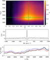 |
Fig. 10. Detection plots for the secondary companion of the binary PX Vir. In the lower panel, the black line with gray error curves corresponds to the adopted solution, which has been calculated with a template of Teff, B = 4000 K and v sin i = 4 km s−1. In the blue line solution, the projected rotation has been changed to 8 km s−1, while in the red line solution, the template temperature has been increased to 4300 K. |
The reconstructed spectrum has an S/N above 10–15 in the red, which is high enough to clearly recognize the spectral morphology in a late-type star. Figure 11 compares the spectral morphology of two companions. The temperature of the secondary is clearly lower, showing stronger lines of Ti I and Mn I, compared with the primary. In fact, the presence of molecular features in the spectrum suggests that the temperature is somewhat lower than obtained by our program, probably close to 3900 K.
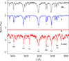 |
Fig. 11. Disentangled spectra of the components of PX Vir. From top to bottom: One of the observed spectra (black), the reconstructed spectrum of the primary (blue), the spectrum of the secondary (red), and the secondary spectrum multiplied by 23. Arbitrary vertical shifts have been applied for better visibility. |
Once the secondary spectrum has been reliably obtained and its velocity estimated, an ordinary iterative disentangling can be performed with the method of González & Levato (2006). The obtained RV curve is shown in Fig. 12. We note that the application of the task find2c was necessary to get to the solution, as there were no detectable secondary features in either the individual observed spectra or in the correlation function. The mass ratio value derived from these RV curves is q = 0.596 ± 0.005, consistent with, and more precise than, the values published by Cusano et al. (2009) and Wang et al. (2023).
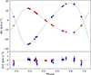 |
Fig. 12. RV curve of the primary (blue) and secondary (red) companions of PX Vir. The bottom panel shows the residuals observed minus the ones calculated. |
7. Discussion
We have proposed a technique to reinforce the signature of the secondary companion in the spectrum of binary stars in order to derive the mass ratio in systems classified as SB1s. The method is a combination of the iterative disentangling used in an automatic blind way in combination with cross-correlations with a grid of spectral templates. There are two free parameters to be optimized: the mass ratio and a parameter specifying the template morphology of the secondary star (Teff, B in our case).
For the calculations, it is assumed that both RV curves correspond to Keplerian orbits around the same center of mass and that the spectral morphology of the stars does not vary. Although in practice this is valid for most binary stars, there are exceptions. It would not be possible, for example, to detect very faint companions when the primary is an intrinsically variable or a spotted star. In the case of eclipsing binaries, the spectra taken during the eclipses should be excluded from the analysis to avoid variations in the relative line intensity, and eventual distortions of the line profiles due to the Rossiter-McLaughlin effect. The presence of other spectral components – for example, a fixed line set from a third star or some circumstellar structure – would also hamper a neat spectral disentangling. We also note that Eq. (1) is strictly valid only if the difference in the gravitational redshift of the two stars is negligible. While this difference is as large as a few tens of km s−1 in binaries with a white dwarf component (e.g., Koester 1987), it is negligible if both components are main-sequence stars and on the order of only half a km s−1 in dwarf+giant binaries (e.g. El-Badry 2022). In any case, this fact does not represent any limitation to the method applicability, since an RV correction can easily be added to Eq. 1 according to the expected difference (e.g., when the primary is a red giant).
From experiments with artificial spectra, we found that the larger the rotational broadening of the object spectrum, the smaller the calculated scaling factor, α. Moreover, large differences in spectral type also result in scalling factors that are too small. This latter effect is not symmetric, being more pronounced when the object is hotter than the template. In fact, in some cases, objects with temperatures 100–200 K lower showed errors in excess. This is because in FGK-type stars a small temperature decrease causes a global enhancement of metallic lines, so an object that is slightly cooler than the reference spectrum would appear to have a larger α.
We have shown that from standard-quality spectral datasets it is possible to detect the secondary star in systems in which the secondary contributes less than 0.5–1.0% of the total flux. The best results are obtained for binaries in which the secondary has a relatively late spectral type with many useful spectral lines. This is satisfied even in early-B type SB1s, in which the secondary is probably a late-A or F-type star. Secondaries with a high rotational velocity might be difficult to detect. The potential field of application is very wide, and a significant contribution can be made to binary statistics by incorporating a large number of low-mass-ratio systems. Suitable targets – that is, SB1s with mass ratio high enough to be detected with the proposed technique – can be selected on the basis of the primary RV curve. Specifically, from the mass function derived from the RV curve and an estimate of the primary mass, a lower limit for the secondary mass can be calculated. If we assume that the secondary companion is a main-sequence star, then a lower minimum of the light-ratio can be derived.
As an exploratory exercise, we selected in the SB9 catalogue (Pourbaix et al. 2004) those systems whose primary is known to be a main-sequence star. This restriction allowed us to use a known mass-luminosity relation to translate the mass ratio into a visual light-ratio. Using the orbital parameters and assuming a limit in the brightness difference of 6 mag, we found that there would be more than 600 SB1s for which it should be possible to measure the mass ratio. This would be almost double the number of binaries with a measured mass ratio in the catalogue mentioned.
The eventual non-detection of the secondary might have some interesting implications in some systems. A negative result sets an upper limit to the secondary star flux and, if we assume that the companion is a main-sequence star, this establishes an upper limit for its mass. In case this upper limit is lower than the minimum secondary mass derived from the mass function, then no main-sequence star can satisfy both observational restrictions. In other words, if we can impose a strict limit on the brightness of a star that is rather massive, then we can infer that we are dealing with a compact companion; that is, a white dwarf or a neutron star. This can be considered as a method of searching for binaries with a compact component.
A natural application field for this technique is the characterization of binary stars with low-mass companions. In Paper II, by Martínez & González (in prep.), we analyze a sample of K and M-type binary candidates, identifying a few systems with secondaries below 0.2 M⊙. In that paper, more technical details of the method are given and a PYTHON-based program is made publicly available.
We used ESO archive data corresponding to programs 075.C-0202(A), 076.C-0010(A), 077.C-0012(A), 079.C-0046(A), and 083.C-0794(D).
Acknowledgments
Based on data acquired at the Complejo Astronómico El Leoncito, operated under agreement between the Consejo Nacional de Investigaciones Científicas y Técnicas de la República Argentina and the National Universities of La Plata, Córdoba and San Juan. It is also based on observations collected at the European Southern Observatory under programs IDs: 075.C-0202(A), 077.C-0012(A), 076.C-0010(A), 079.C-0046(A), and 083.C-0794(D) This work was partially supported by CONICET of Argentina, through grant PIP11220170100331CO.
References
- Bressan, A., Marigo, P., Girardi, L., et al. 2012, MNRAS, 427, 127 [NASA ADS] [CrossRef] [Google Scholar]
- Coelho, P., Barbuy, B., Meléndez, J., Schiavon, R. P., & Castilho, B. V. 2005, A&A, 443, 735 [NASA ADS] [CrossRef] [EDP Sciences] [Google Scholar]
- Cusano, F., Guenther, E. W., Esposito, M., et al. 2009, in AIP Conf. Ser., 1094, 788 [NASA ADS] [CrossRef] [Google Scholar]
- Dahm, S. E. 2005, AJ, 130, 1805 [NASA ADS] [CrossRef] [Google Scholar]
- El-Badry, K. 2022, Res. Notes Am. Astron. Soc., 6, 137 [Google Scholar]
- Evans, T. M., Ireland, M. J., Kraus, A. L., et al. 2012, ApJ, 744, 120 [NASA ADS] [CrossRef] [Google Scholar]
- Gaia Collaboration (Vallenari, A., et al.) 2023, A&A, 674, A1 [NASA ADS] [CrossRef] [EDP Sciences] [Google Scholar]
- González, J. F., & Levato, H. 2006, A&A, 448, 283 [NASA ADS] [CrossRef] [EDP Sciences] [Google Scholar]
- González, J. F., & Levato, H. 2009, A&A, 507, 541 [NASA ADS] [CrossRef] [EDP Sciences] [Google Scholar]
- Griffin, R. F. 2010, The Observatory, 130, 125 [NASA ADS] [Google Scholar]
- Griffin, R. F. 2013, The Observatory, 133, 322 [NASA ADS] [Google Scholar]
- Hogeveen, S. J. 1992, Ap&SS, 196, 299 [NASA ADS] [CrossRef] [Google Scholar]
- Houk, N. 1982, Michigan Catalogue of Two-dimensional Spectral Types for the HD stars. Volume_3. Declinations -40o to -26o (Dept. of Astronomy, University of Michigan) [Google Scholar]
- Hut, P. 1981, A&A, 99, 126 [NASA ADS] [Google Scholar]
- Koester, D. 1987, ApJ, 322, 852 [NASA ADS] [CrossRef] [Google Scholar]
- Moitinho, A., Alves, J., Huélamo, N., & Lada, C. J. 2001, ApJ, 563, L73 [NASA ADS] [CrossRef] [Google Scholar]
- Nguyen, C. T., Costa, G., Girardi, L., et al. 2022, A&A, 665, A126 [NASA ADS] [CrossRef] [EDP Sciences] [Google Scholar]
- Pourbaix, D., Tokovinin, A. A., Batten, A. H., et al. 2004, A&A, 424, 727 [NASA ADS] [CrossRef] [EDP Sciences] [Google Scholar]
- Straizys, V., & Kuriliene, G. 1981, Ap&SS, 80, 353 [CrossRef] [Google Scholar]
- Trifonov, T., Tal-Or, L., Zechmeister, M., et al. 2020, A&A, 636, A74 [NASA ADS] [CrossRef] [EDP Sciences] [Google Scholar]
- van Leeuwen, F. 2007, A&A, 474, 653 [CrossRef] [EDP Sciences] [Google Scholar]
- Wang, X., Xia, F., & Fu, Y. 2023, PASJ, 75, 368 [NASA ADS] [CrossRef] [Google Scholar]
All Tables
All Figures
|
Fig. 1. Flux contribution of the secondary companion as a function of binary mass ratio. Four models are shown: a primary of 10 M⊙ (thin lines) and 2 M⊙ (thick lines) for ages close to the primary terminal-age main-sequence (solid lines) and about half the main-sequence lifetime (dashed). |
| In the text | |
|
Fig. 2. Detection plots for the secondary companion in a synthetic example. a) One of the 20 artificial binary spectra of the demonstration example. The “observed” composite spectrum (black) is compared with component synthetic spectra (primary in blue, secondary in red) to show the intensity of the secondary lines. The lower spectra have been multiplied by 50 for better visibility. Arbitrary vertical shifts have been applied. b) SSF in the q − Teff plane. Green lines mark the position of the maximum and next to both axes the corresponding cross-sections defining the best solution (Teff = 4000 K, q = 0.37) are shown. c) Reconstructed secondary spectrum (black) compared with a synthetic noise-free spectrum of 4000 K (red). d) Cross-correlation function corresponding to the adopted solution. |
| In the text | |
|
Fig. 3. Frontier between SB1s and SB2s. In the upper region (labeled SB2), the spectral lines of the secondary are visible in individual spectra. Between the black and the green curves, the spectral lines of the secondary are not distinguishable in individual spectra but they are clearly seen in the reconstructed spectrum of the secondary, in which the S/N is increased by a factor equal to the square root of the number of observations. Above the red line, the peak of the cross-correlation function is high enough to measure RV in individual spectra. The region labeled with “q measurable” corresponds to configurations in which it is not possible to measure RVs for the secondary star nor to study the spectral morphology of the spectrum, but still it is possible with our technique to calculate the mass ratio. |
| In the text | |
|
Fig. 4. Detection plots for star W57. Top: SSF in the q − Teff plane. The vertical green line marks the lower limit of q according to the spectroscopic mass function and an estimated primary mass of 1.4 M⊙. The yellow line shows the temperature for each possible value of the secondary mass, assuming it is a main-sequence star of the age of the cluster. Bottom: Cross-correlation function of the reconstructed secondary spectrum for several experiments adding artificial secondaries to the observed spectra. The inset shows the contribution of the secondary star to the total flux. |
| In the text | |
|
Fig. 5. Detection plots for the secondary companion of the binary W61 (left) and w86 (right). From top to bottom: Secondary detection function in the q − Teff, B plane, cross-correlation function for the best B spectrum, and estimated flux contribution of the secondary star. |
| In the text | |
|
Fig. 6. Color-magnitude of the open cluster Blanco 1 in the Gaia photometric system. Squares (triangles) mark the location of the primary (secondary) components of the three studied binaries: w57 (green), w61 (red), and w86 (blue). The gray line marks the magnitude limit of the instrument for a spectrum of S/N = 100 in a 1-hour exposure. |
| In the text | |
|
Fig. 7. Region of CASLEO spectra of the binary NGC 2362-46 showing He I lines at λλ4387, 4438, 4471 and the Mg II line at λ4481. The spectra are ordered by phase and shifted vertically for better visibility. Note that the RV amplitude is significantly smaller than the width of spectral lines. |
| In the text | |
|
Fig. 8. RV curve of NGC 2362-46. The lower panel shows the residuals of the orbital fit. |
| In the text | |
|
Fig. 9. Detection plots for the secondary companion of the binary NGC 2362-46. |
| In the text | |
|
Fig. 10. Detection plots for the secondary companion of the binary PX Vir. In the lower panel, the black line with gray error curves corresponds to the adopted solution, which has been calculated with a template of Teff, B = 4000 K and v sin i = 4 km s−1. In the blue line solution, the projected rotation has been changed to 8 km s−1, while in the red line solution, the template temperature has been increased to 4300 K. |
| In the text | |
|
Fig. 11. Disentangled spectra of the components of PX Vir. From top to bottom: One of the observed spectra (black), the reconstructed spectrum of the primary (blue), the spectrum of the secondary (red), and the secondary spectrum multiplied by 23. Arbitrary vertical shifts have been applied for better visibility. |
| In the text | |
|
Fig. 12. RV curve of the primary (blue) and secondary (red) companions of PX Vir. The bottom panel shows the residuals observed minus the ones calculated. |
| In the text | |
Current usage metrics show cumulative count of Article Views (full-text article views including HTML views, PDF and ePub downloads, according to the available data) and Abstracts Views on Vision4Press platform.
Data correspond to usage on the plateform after 2015. The current usage metrics is available 48-96 hours after online publication and is updated daily on week days.
Initial download of the metrics may take a while.