| Issue |
A&A
Volume 694, February 2025
|
|
|---|---|---|
| Article Number | A32 | |
| Number of page(s) | 16 | |
| Section | Stellar structure and evolution | |
| DOI | https://doi.org/10.1051/0004-6361/202451496 | |
| Published online | 30 January 2025 | |
BiSpeD: Binary Spectral Disentangling applied to binary low-mass star searches
1
Observatorio Astronómico Félix Aguilar, Universidad Nacional de San Juan, Av. Benavidez Oeste, 8175 San Juan, Argentina
2
Instituto de Ciencias Astronómicas de la Tierra y el Espacio (CONICET-UNSJ), Av. España 1512 sur, San Juan, Argentina
⋆ Corresponding authors; This email address is being protected from spambots. You need JavaScript enabled to view it.
, This email address is being protected from spambots. You need JavaScript enabled to view it.
Received:
13
July
2024
Accepted:
18
December
2024
Abstract
Context. In a companion paper, we present a novel method for the spectroscopic detection of low-luminosity secondary companions of binary stars. An interesting application field is the identification of very low-mass stars as companions of late-type main-sequence stars.
Aims. To provide a simple tool based on our method, we developed Binary Spectral Disentangling (BiSpeD), a PYTHON repository that provides a toolkit for processing and analyzing spectroscopic observations. The main task of BiSpeD is find2c, which aims to calculate the mass ratio (q) of a single-lined spectroscopic binary from the analysis of a sample of observed spectra. In the same process, an estimate of the secondary effective temperature is obtained. In addition, the toolkit includes other spectral measurement tasks, including spectral disentangling and radial velocity (RV) measurement via cross-correlation.
Methods. The BiSpeD package was tested on a sample of 41 late-type stars observed by the High-Accuracy Radial Velocity Planetary Searcher (HARPS). For each star in the sample, we measured the RV for the primary companion and determined the orbital parameters. We then applied the find2c task, which defines a grid of mass ratios and generates the corresponding grid of solutions that reconstruct the secondary spectrum using iterative spectral disentangling. Finally, a modified cross-correlation algorithm compares these secondary spectra with synthetic templates to find the best solution.
Results. Our analysis led to the detection of 12 faint companions from the 41 candidates, including five stars below 0.3 M⊙. Among our positive detections are two cases of binaries formed by a red giant primary and a main-sequence secondary. We show that reliable mass ratio values can be obtained even in cases where the orbital period is unknown and the RV amplitude is only a few km s−1.
Key words: binaries: spectroscopic / stars: low-mass
© The Authors 2025
 Open Access article, published by EDP Sciences, under the terms of the Creative Commons Attribution License (https://creativecommons.org/licenses/by/4.0), which permits unrestricted use, distribution, and reproduction in any medium, provided the original work is properly cited.
This article is published in open access under the Subscribe to Open model. This email address is being protected from spambots. You need JavaScript enabled to view it. to support open access publication.
1. Introduction
The stellar and substellar mass distribution is crucial for understanding the link between stellar and galactic evolution (Scalo 1986). Very low-mass stars (VLMSs), usually defined as M dwarfs with masses of less than 0.6 M⊙ (Chen et al. 2014) or 0.8 M⊙ (Chabrier & Baraffe 1997), are the dominant population in the Galaxy because they form in large numbers and have lifetimes longer than that of the Universe. According to current measurements of the initial mass function (Li et al. 2023; Kirkpatrick et al. 2024), VLMSs account for more than 80% of the stars and about one-third of the total stellar mass.
The most important tool for the direct determination of mass and other stellar parameters has been and still is the analysis of binary stars, in particular the spectroscopic-photometric study of eclipsing binaries and the spectroscopic-astrometric study of visual binaries (Serenelli et al. 2021). In the case of VLMSs, however, their low intrinsic brightness makes their detailed study more challenging, and it is only in recent years that significant progress has been made in our empirical knowledge of them, thanks in large part to their importance for planet detection. In fact, during the last two decades of the 20th century, YY Gem and CM Dra remained the only two known eclipsing binaries with very low-mass components (see the review by Ribas 2006, and references therein), while the recent compilation by Morales et al. (2022) collected 32 eclipsing binaries with at least one very low-mass component measured with an error of less than 3%.
The observed masses and radii of low-mass stars show significant discrepancies with current stellar models. For M-type main-sequence stars, around the transition between stars with radiative cores and those that are fully convective, the observed stellar radii are larger than predicted by models. This is a long-standing controversy (see for example Ribas 2006; López-Morales 2007; Triaud et al. 2013; Chen et al. 2014, and references therein), sometimes referred to as the “M dwarf radius inflation problem”, and it remains an open question (Swayne et al. 2024; Davis et al. 2024). Fortunately, the empirical mass-luminosity relation shows better agreement with models (Ribas 2006) and, most importantly, little scatter and no significant dependence on metallicity, especially when using infrared flux (e.g., mass vs. absolute magnitude in the Ks band; Benedict et al. 2016; Mann et al. 2019). A reliable calibration of the mass-luminosity relation is crucial, as it is the key to estimating masses for individual VLMSs and mass ratios in visual binaries.
Typically, binary systems with VLMSs as secondary companions are studied from the radial velocity (RV) variation of a primary component or, in the case of eclipsing binaries, transits. The large luminosity difference between components of different masses in binary systems makes it difficult to characterize the spectrum of the fainter companion (e.g., Triaud et al. 2013).
In fact, for binaries with a mass ratio of q ≲ 0.5, the flux ratio is usually low enough that the spectral features of the secondary star are hidden by the observational noise of the spectra. Secondary signal detection in these difficult cases is precisely the main goal of the technique presented in this and a companion article (González et al. 2024, hereafter referred to as Paper I). In Paper I we describe the basics of the method, which is further developed here and applied to the detection of low-mass stars. Specifically, this paper presents Binary Spectral Disentangling (BiSpeD), a toolkit for spectroscopic analysis developed in PYTHON. The toolkit implements a new technique for the detection of faint secondary stars in spectroscopic binaries by means of functions (hereafter referred to as “tasks”), in addition to some other tools for the handling and analysis of binary star spectra. To test the BiSpeD code, we applied it to search for low-mass stars among the secondary companions of spectroscopic late-type binaries. In Sect. 2 we describe the structure of the toolkit; in Sect. 3 we test BiSpeD on a synthetic spectroscopic observation dataset to demonstrate its application. In Sect. 4 we describe the High-Accuracy Radial Velocity Planetary Searcher (HARPS) sample selection and the template grid. In Sect. 5 we present the results for our sample of stars, and in Sect. 6 we discuss the main results of our work and draw some conclusions.
2. Package structure
BiSpeD is a toolkit for spectroscopic analysis, presented as a PYTHON repository. BiSpeD works through specific functions (tasks) for manipulating and processing spectroscopic observations of binary stars. In alphabetical order, the tasks currently available are:
-
find2c: estimate the mass ratio and temperature for the secondary component of a binary star for which the secondary lines are not easily detectable in the spectrum;
-
hselect: extract header information;
-
onecomp: compare a single object spectrum to a set of templates and find the best match;
-
rvbina: measure the RV of the components of a double-lined spectroscopic binary (SB2) after removing the companion features;
-
rvextract: analyze the convergence of the RV measurements obtained with rvbina in the context of iterative disentangling;
-
setrvs: measure RVs using cross-correlations;
-
spbina: reconstruct the spectra of the component of a binary star using iterative disentangling;
-
splot: plot a spectrum;
-
uniform: renormalize a series of spectra to a common continuum;
-
vgrid: run find2c for a grid of center of mass velocities;
-
vexplore: visualize the results of the vgrid analysis.
The main task of find2c is to find the best solution of the mass ratio and effective temperature of the secondary companion of a spectroscopic binary from a given spectral dataset. The input binary spectra (a set of 1D image spectra in FITS format) do not need to be continuum normalized, but the continuum shape should to be the same for all of them so that they are morphologically consistent. If this is not the case, a re-normalization to a common continuum can be easily performed using the uniform task.
The basics of the find2c methodology are described in detail in Paper I, but for convenience we summarize the main features here and add some more technical details. First, find2c combines the observational data of the binary and calculates the secondary mean spectrum Bq for a grid of mass ratios (q values) as possible solutions to the system. These calculations are performed through an iterative disentangling technique (González & Levato 2006) using the task spbina, and require preliminary values of the RV of both components.
Therefore, before find2c is run, the primary RV must be measured using any method, for example by cross-correlation using the BiSpeD task setrvs, which automatically records the results in the image header. This task computes the cross-correlation between two spectra using the Fast Fourier Transform method to perform the convolution. The most notorious peak of the cross-correlation function is fitted with a Gaussian function. The standard error of the fit is calculated using the diagonal covariance matrix (Anglada-Escudé & Butler 2012) and the final RV error is estimated using a procedure similar to Tonry & Davis (1979).
Specifically designed to analyze objects classified as single-lined spectroscopic binaries (SB1s), find2c assumes no prior information about the secondary star and uses the RV measurements of the primary star (VA) to derive the corresponding values for the secondary component (VB), such as
 (1)
(1)
where γ is the systemic RV and q ≡ MB/MA is the mass ratio. This expression is easily derived from the definition of the center of mass velocity:
 (2)
(2)
Although the orbital period is not used in any calculation, the primary spectroscopic orbit should be fitted to obtain the center-of-mass velocity γ. However, in cases where the orbital period is unknown, an alternative strategy for estimating γ can be used by applying the vgrid task, as described below.
For each mass ratio, the spectrum representing the secondary companion (Bq) is constructed by combining the observed spectra after the appropriate RV shift and removal of the spectral features of the primary component. In order to minimize the processing time when running find2c, the calculation of the spectra Bq is done by parallelizing the execution of the task spbina over multiple q-values.
In a second step, find2c calculates the secondary significance function (SSF) as the normalized product of the spectra Bq and the template series:
 (3)
(3)
where ⟨⟩ is the mean and Bmax is the secondary spectrum with the largest flux variance. This expression is a numerical method for solving Eq. (2) of Paper I, which is essentially the classical cross-correlation function evaluated at zero velocity shift. Prior to cross-correlation, the Bq and template spectra are rectified by subtracting a fit of the continuum using a Chebyshev polynomial function. The best solution (i.e., the optimal mass ratio and secondary temperature) is determined from the location of the maximum of the SSF.
3. Code testing
For the purpose of evaluating the accuracy of BiSpeD results, we developed an open access tool (ssynth1) to generate synthetic spectroscopic observational datasets of a simulated binary system. The dataset is built from any two component spectra and orbital parameters provided by the user. The parameters of ssynth are: number of observations (N), flux ratio (LB/LA), mass ratio (MB/MA), orbital period (P), spanning time, tilt angle (i), RV measurement random error, and S/N (as Gaussian noise added to the composite spectrum).
Next, we tested BiSpeD in numerous experiments with different parameter combinations. To make our artificial binaries look like the candidates we would extract from the public HARPS database, we first made a statistic of the characteristics of the spectra in that database. We used S/N in the range of 50–200, which is typical for the spectra in the HARPS database. We chose N varying from 6 to 25 to ensure a minimum number of spectra at different phases (or more precisely, at different velocities). To test the application of the code to data samples with velocity uncertainties greater than those of HARPS, we added random shifts with amplitudes ranging from 0.1 to 0.5 km s−1 to the synthetic binary spectra. We expected to find low-mass secondary companions with LB/LA in the range of 0.001–0.1, and MB/MA in the range of 0.1–0.9, according to Fig. 3 of Paper I. We therefore chose a range of orbital periods P from 50 to 1000 d; corresponding to primary RV amplitudes from 5.4 km s−1 (for P = 50 d and i = 90°) to 1 km s−1 (for P = 1000 d and i = 30°) for a binary of MB/MA = 0.1. Since spectral disentangling is more effective at higher RV amplitudes, we decided not to test for orbital periods of less than 50 d. We note that the orbital period does not directly affect the results, but defines the amplitude of the RV curve.
Considering our main goal, several spectra were used as input: synthetic templates from the library of Coelho et al. (2005), from the Göttingen Spectra Library, and also observed HARPS spectra of single stars (HD 15411 and GJ 1012). Within this mentioned parameter space, we identified the conditions under which the code can detect the secondary companion of SB1 stars for HARPS spectra. We have found that BiSpeD analysis can detect the secondary component and recover the mass ratio with an accuracy of 0.01 when the following conditions are simultaneously satisfied: K > 1 km s−1, LB/LA > 0.003, and N > 8 (modeled with spectra of HD 15411 as primary and GJ 1012 as secondary). For instruments with a lower resolving power, the limiting RV amplitude is expected to be proportionally larger.
As discussed in Paper I, the method is applicable to stars of all spectral types but is particularly effective when the secondary is a late-type star with many useful spectral lines. This is, of course, the case for late-type binaries.
We show the results for a synthetic example for which we modeled an observational dataset consisting of 25 spectra spanning 8 years. The input binary consists of two stars with masses MA = 0.68 M⊙ and MB = 0.22 M⊙. Using the spectral calibration of Pecaut & Mamajek (2013) in its online version2, we assigned effective temperatures and luminosities to build the component spectra. The stellar parameters correspond approximately to spectral types K5 V for the primary and M5 V for the secondary, with temperatures of 4400 K and 3200 K, and a luminosity ratio of 0.036. We used HARPS spectra of late-type stars to build the synthetic observations. The orbit was assumed to have a period of P = 200 d and an inclination angle of i = 90, resulting in a primary RV curve with a semi-amplitude of KA = 8.59 km s−1. Finally, we added photon noise to each synthetic binary spectrum to achieve a S/N of about 150. To illustrate, in Fig. 1 we show a spectrum and its corresponding template for the primary component.
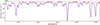 |
Fig. 1. Example of one of the synthetic spectra associated with the modeled binary (red) and a spectrum template of the effective temperature Teff = 4400 K (blue). The spectral features correspond to the primary component; the spectral features of the secondary companions cannot be seen due to the noise level added in the modeled synthetic binary. |
We run the find2c task using the Göttingen Spectra Library as the template grid. (Husser et al. 2013) based on Phoenix atmosphere models for effective temperatures from 2300 K to 7000 K and log g from +1.0 to +6.0. The results are presented in a dynamic graphical user interface (GUI) as a 3D density plot (Fig. 2), with the mass ratio on the X-axis, the effective temperatures on the Y-axis, and the SSF-value on the Z-axis. Additionally, two other plots are shown: ℱ(q, Teff) as a function of mass ratio for the best effective temperature and as a function of effective temperature for the best mass ratio. In this work, we used different template grids corresponding to different log g values. In Fig. 3 we show ℱ(q, Teff) for different log g. It can be seen that the mass ratio (q) found by BiSpeD does not depend on log g, but the effective temperature does. We believe that log g is not a parameter that can be derived by this type of analysis, while the temperature value should be considered only as an estimate. In the example of Fig. 3 the estimated effective temperature varies from 3100 K to 3500 K and the maximum of ℱ (at 3500 K) corresponds to log g = +3.0. However, all solutions are consistent with respect to the mass ratio, giving the same q value within the grid step (0.01) in all cases with log g between +1.0 and +5.0. We therefore consider the mass ratio determination to be robust.
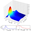 |
Fig. 2. GUI 3D standard output of the find2c analysis over the synthetic example. Top: 3D density plot for the SSF. Bottom left: Mass ratio cross section for the best effective temperature peak. Bottom right: Effective temperature cross section for the best mass ratio. For the maximum ℱ peak the values are q = 0.32 and Teff, B = 3300 K (marked by dotted gray lines). |
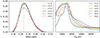 |
Fig. 3. BiSpeD analysis of the synthetic example correlated with different template grids; the colors correspond to the log g used. Left: Mass ratio cross section for the best effective temperature peak. Right: Effective temperature cross section for the best mass ratio. |
A similar behavior was observed for the real binaries analyzed in Sect. 5 when using different template grids. When reporting the results, we mentioned the log g corresponding to the grid that gave the highest SSF-value, even though we expect all detected secondary components to be main-sequence stars.
If the orbital period cannot be derived from the primary RVs, and therefore the center of mass velocity is unknown, the vgrid task can be used to estimate the binary systemic RV. This task runs find2c through a grid of systemic velocities and searches for the best solution. The γ grid is defined by the user, usually considering a reasonable interval around the mean RV or including the entire range between the maximum and minimum values among the measured RVs. In the example shown in Fig. 1, the systemic velocity was fixed at its input value of γ = 0 km s−1. In a second run, the vgrid task was applied to a grid of γ values between −2.5 and 3.0 km s−1. In Fig. 4 a sequence of 3D function density ℱ(q, Teff) for different systemic velocities is shown. The input value is clearly recovered.
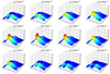 |
Fig. 4. 3D density plot for ℱ(q, Teff) for increasing values of the systemic velocities from γmin = −2.5 km s−1 on the top left to γmax = 3.0 km s−1 on the bottom right, in steps of 0.5 km s−1. The best solution is γ = 0 km s−1. |
4. Star sample and input data
To select candidates for binaries with low-mass secondaries, we searched for late-type stars observed with the HARPS, a fiber-fed echelle spectrograph mounted at the European Southern Observatory (ESO) on the 3.6m telescope at La Silla, Chile (Pepe et al. 2002; Mayor et al. 2003). HARPS has a fiber aperture of 1 arcsec on the sky. The resulting spectra cover the wavelength range 3800–6900 Å with a resolving power of R = 115 000. This instrument is optimized for stellar RV measurements with an excellent accuracy down to 1 m s-1 due to its stability on yearly timescales (Wildi et al. 2010). The Data Reduction Software of HARPS provides precise RV measurements derived from cross-correlations (see Pepe et al. 2002, for more details). However, Trifonov et al. (2020) has performed an independent systematic RV analysis with higher accuracy. This catalog contains more than 212 000 RV measurements for about 3000 stars observed from 2003 to 2018, along with auxiliary information about the method. We selected our sample from this catalog by filtering stars with spectral types between K0 and M7, with more than eight observations, and with an RV amplitude ΔRV > 1 km s−1. We excluded stars classified as SB2s. Using these criteria, we obtained 41 candidates for SB1s listed in Table 1, of which only 11 were classified as spectroscopic binaries in SB9 Catalog (Pourbaix et al. 2004). The sample dataset was obtained from the ESO archive using the generic query3.
Sample of HARPS low-mass binary candidates.
In Fig. 5 we show the color-magnitude diagram of our sample, using data from the Gaia Data Release 3 (DR3) catalog (Gaia Collaboration 2023). The correction for the interstellar absorption Ad(G) in the G band was estimated using the calibration of the G-band extinction coefficient kG = Ad(G)/Ad(V) by Danielski et al. (2018) and the visual extinction Ad(V) calculated using the model described by Bahcall & Soneira (1980):
![Mathematical equation: $$ \begin{aligned} A_d(V) = A_{\infty }(b) \left[ 1 - e^{-| d \sin {b} |/{H}}\right], \end{aligned} $$](/articles/aa/full_html/2025/02/aa51496-24/aa51496-24-eq4.gif) (4)
(4)
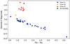 |
Fig. 5. HR diagram of a sample of stars. Stars are colored according to their luminosity class: V (blue), IV (orange), III (red), and unclassified (green). |
where d is the distance, A∞(b) is the total interstellar absorption for a galactic latitude b (six objects from the list have b < 5 deg, but we have included them in the Hertzsprung–Russell (HR) plot to show the distribution of the star sample), and H = 100 pc is the scale height taken from Marshall et al. (2006).
For the spectra taken before 2018, we extracted the RV values from the catalog of Trifonov et al. (2020). For the most recent spectra we measured the RV with our task setrvs. In most cases, we fitted the RV curve orbit using the formalism of Delisle et al. (2016) to get a first estimate of the orbital parameters, and then performed a mean square fit of the RV curves to get the γ parameter required by the find2c task. In cases where the period could not be unambiguously identified, the vgrid strategy was used.
We applied the find2c task using a template grid built from synthetic spectra with Teff in the range 2300–6300 K and log g from +1.0 to +6.0, taken from the Göttingen Spectral Library. For the calculation of ℱ, we defined a working spectral region with several windows excluding broad features, lines that often show emission cores, the instrumental gap near λ5300, and telluric lines. The default spectral region of BiSpeD was set to 4000–4090 Å, 4110–4320 Å, 4360–4850 Å, 4875–5290 Å, and 5350–5880 Å.
5. Results
We list the main orbital parameters computed from the RV curve fitting for 12 objects with definite solutions (Table 2), for which the SSF peak was at least ten times the RMS of the noise. The RV fits are shown in Appendix A. The resulting mass ratios (q) and the effective temperature (Teff, B) of the best template are listed in Table 3.
Orbital parameters.
BiSpeD detections.
The assigned uncertainties in q were calculated by the bootstrap method. We ran the find2c analysis 100 times on samples of spectra taken randomly from the original dataset with replacement. We would like to clarify that the effective temperature is not a calculated value, but only the temperature of the template with the maximum cross-correlation. To estimate an uncertainty value, we need to express it in terms of the grid step, that is, the probability of obtaining the maximum SSF for the nearby templates. For 10 out of 12 objects, the bootstrap runs typically fell on the same bin (±100 K), so we adopted the temperature step as the formal uncertainty. The only exceptions are HD 127124, for which the standard deviation was larger (±200 K), and HD 96118, for which we used a different template grid with a spacing of 250 K. A proper discussion of the reliability of the effective temperature and a realistic estimation of its uncertainty would require the use of a template library with a finer temperature grid and the consideration of possible differences between object and templates in other relevant parameters (abundances, log g, rotation).
In addition, a minimum mass for the secondary companion has been calculated as follows:
 (5)
(5)
where G is the gravitational constant. We note that this minimum secondary mass depends only on the spectroscopic orbital parameters.
An estimate of the primary component mass was obtained from the position of the stars in the color-magnitude diagram. We interpolated the Gaia absolute magnitude and intrinsic color (Fig. 5) into the PARSEC stellar model grid (Chen et al. 2014; Nguyen et al. 2022). These models have been calibrated with empirical data to provide a good fit especially for low-mass stars (Chen et al. 2014). The resulting masses are listed in the fourth column of Table 3. We used isochrones for the solar composition for all stars except two objects with metallicities significantly (more than 0.1 dex) different from 0.0: HD 4457 (Fe/H = − 0.37, Soubiran et al. 2022) and Wolf 414 (Fe/H ∼ + 0.2, Gaidos et al. 2014; Kuznetsov et al. 2019). All stars except HD 96118 are nearby objects (≲100 pc), so parallax and extinction uncertainties have little effect (≲1 − 2%) on the primary mass estimates. In the following discussion of individual systems, we used the published values for the primary mass when available, and otherwise the values estimated from the position in the color-magnitude diagram.
Below we comment on each target and plot the results. For each target, we plot the SSF as a 2D density plot in place of the standard GUI 3D output of find2c. Additionally, we plot cross sections along both axes (q and Teff) and the cross-correlation function corresponding to the best solution (Appendix B).
As a first example, we include a non-detection case to illustrate the limitations of this type of analysis with an insufficient S/N. This is star CD-45 7872, a late-type star classified as M1 V by Koen et al. (2010), with V = 11.096 and Teff = 3543 K (Andrae et al. 2018). Zechmeister et al. (2009) classified this system as SB1 and reported a period of 243 d, but with a high false alarm probability. In addition, they derived a stellar mass MA = 0.54 M⊙ for the primary companion from the K-band mass-luminosity relation of Delfosse et al. (2000). Later, Tuomi et al. (2014) found evidence of a massive substellar companion whose orbit could not be constrained.
In Fig. 6 we show our orbital fitting with the parameters P = 587.179 d, KA = 4.10 km s−1, and e = 0.410. Our orbital fit is consistent with the observations analyzed by Zechmeister et al. (2009), but not with the period they found. Their misidentification of the period was due to the poor phase coverage of the observations available at the time.
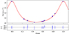 |
Fig. 6. Phase curve of CD-45 7872 for orbital period P = 587.179 d. The RV measurements are shown as blue dots. The bottom panel shows the residuals of the orbital fit. |
Although the BiSpeD analysis yielded a SSF maximum at q = 0.25 and Teff, B = 3300 K, we do not consider this detection reliable since the cross-correlation peak is only 4.44 times the noise σ (see the bottom panel of Fig. 7), which is well below the detection criterion defined in Sect. 3 of Paper I. We therefore considered this to be a case of non-detection with the available observations. The S/N of the HARPS spectra of this object is relatively low (∼30), and a much larger number of observations would be needed to reach the S/N required for positive detection.
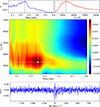 |
Fig. 7. Example of a non-detection case for the star CD-45 7872. Top: Cross sections of the SSF as a function of the mass ratio, q (left) and the effective temperature of the secondary companion, Teff, B (right). Middle: 2D density plot for ℱ; the best solution corresponds to q = 0.25 and Teff, B = 3300 K. Bottom: Cross-correlation function between the best secondary spectrum, Bq = 0.25, and a template of 3300 K. |
The secondary companion is expected to be a VLMS. According to its spectral type, the primary star has a mass of about 0.53 M⊙, so if the mass ratio were close to 0.25, the secondary mass would be 0.14 M⊙, a value very close to the lower limit imposed by the mass function (0.12 M⊙).
5.1. CD-35 15144
is a V = 10.2 magnitude K3 main-sequence star (Upgren et al. 1972). Andrae et al. (2018) have estimated the effective temperature of the primary component to be 4840 K. Sousa et al. (2011) included this object in a sample of stars, supposedly clean of known binaries and variables, constructed for their Jupiter-mass planet search program. Using stellar evolution models, they determined a mass of 0.754 M⊙ for CD-35 15144. A similar result was found by Gomes da Silva et al. (2021), who used the spectral synthesis code MOOG4 to infer the stellar mass from the spectrum. (Sneden 1973) and obtained M = 0.769 ± 0.019 M⊙.
In Fig. A.1 we show the RV curve fit for a period P = 173.532 d, corresponding to a highly eccentric orbit. The BiSpeD analysis found a possible solution for CD-35 15144 with a mass ratio of q = 0.59 for a template of Teff, B = 3800 K and log g = +2.0 (Fig. B.1). Using the mass for the primary component estimated by Gomes da Silva et al. (2021), we calculated the mass of the secondary companion to be MB = 0.454 ± 0.011 M⊙, close to the typical mass for a star with Teff, B = 3700 K (spectral type M0.5V) and larger than the minimum mass MBsin3i = 0.305.
5.2. HD 4457
is a binary star with a primary component of spectral type K2 V, effective temperature Teff = 5016 K, age of 6.13 Gy, and mass M = 0.717 ± 0.019 M⊙ (Gomes da Silva et al. 2021).
This is a very long period system for which the available observations, spanning 14 years, only allow lower bounds to be placed on the RV amplitude and orbital period. Three examples of orbital fits are shown in Fig. A.2. Since we cannot fit a unique Keplerian orbit, we run the vgrid task for the spectral range 4400 − 4850 Å, 4870 − 5160 Å and 5340 − 5880 Å, with γ in the range 35–39 km s−1, and find a possible solution with systemic velocity γ = 37 km s−1, mass ratio q = 0.46, and effective temperature Teff, B = 3800 K for log g = +2.5 (Fig. B.2).
Although the period is unknown, it is restricted to a rather limited range: 9000 d ≲P≲ 15 000 d. On the one hand, the residuals of the RV curve fit rise sharply for periods shorter than 9000 d. On the other hand, the mass of the primary imposes an upper limit on the period. As can be seen in Fig. A.2, the phase coverage is insufficient for the longer period. For solutions with periods longer than about 15 000 d, the spectroscopic parameter MAsin3i significantly (20%) exceeds the estimated mass of the primary.
Using the primary mass estimate from Gomes da Silva et al. (2021), we obtain a secondary companion mass of MB = 0.33 ± 0.01 M⊙. Assuming it is a normal main-sequence star, this mass corresponds to a M3 V star (Teff ≈ 3400 K), slightly cooler than the temperature of the best template (3800 K).
5.3. HD 24706
has an evolved primary component with spectral type K2 III (Houk 1978) and an effective temperature of 4400 K (Liu et al. 2007). Using the Gaia DR3 parallax we estimated the absolute magnitudes MV = 0.71 and MG = 0.36. According to the Modules for Experiments in Stellar Astrophysics (MESA; version v7503; Paxton et al. 2011) for the solar abundances (Choi et al. 2016), these magnitudes and temperatures correspond to a red giant branch star of 1.3 M⊙ and 14.5 R⊙ or a red clump star of 0.9 M⊙ and 14.7 R⊙. Our estimated radius is similar to that obtained by Kervella et al. (2022) from the K-band magnitude, but our mass is significantly smaller than theirs (MA = 2.08 ± 0.10 M⊙).
The BiSpeD analysis yielded as the best solution: q = 0.57, Teff, B = 5100 K, and log g = +3.5. Assuming a primary mass of 1.3 M⊙, the secondary is expected to be a main-sequence star of about 0.74 M⊙. The mass corresponding to the estimated secondary temperature (5100 K) is only slightly higher (0.82 M⊙). In Fig. A.3 we show the phase curve for the Keplerian fit; the BiSpeD results and the cross-correlation function are shown in Fig. B.3.
5.4. HD 96118
is a long period (P = 336.6 d, Mermilliod et al. 2007) binary with a red giant primary component. This star was classified as a spectroscopic binary by Pourbaix et al. (2004), has a spectral type of K3III (Houk & Cowley 1975) and an apparent magnitude V = 7.59. The position in the color-magnitude diagram corresponds to a bright giant star of about 6 M⊙. With such a high-mass primary, the secondary could be a B or A type star. Detecting the secondary companion in this type of binary presents a different challenge than in the other cases we have shown, where the secondary was also a late type star. In this case, the luminosity contrast is due to the large radius of the giant, but the secondary temperature may be significantly higher than that of the primary. Since late-B to early-F secondaries will have fewer and possibly broader spectral lines compared to the primary, it is a good strategy to use earlier templates with a moderate but not zero rotation, and to focus the search on specific spectral regions where early-type stars have intense lines.
We fit a Keplerian orbit and obtain P = 336.660 d, KA = 21.53 km s−1 and e = 0.007 (Fig. A.4). The orbital parameters are consistent with the values estimated by Mermilliod et al. (2007). After finding a marginal detection using our standard procedure, we built another template grid by taking from the library of Coelho et al. (2005) stellar spectra covering the temperature range 4500–13 000 K and convolving them with a rotation profile of width v sin i = 30 km s−1. The spectral region mask was restricted to a few windows including the Mg II line at λ = 4481 Å and a few strong Fe II and Si II lines, more specifically the spectral regions 4110–4140 Å, 4460–4500 Å, and 5000–5100 Å. We found a solution for q = 0.6 and Teff, B = 11 750 K (Fig. B.4). The results show a clear detection peak with a S/N of about 10. In the reconstructed spectrum of the secondary a few spectral lines can be clearly distinguished (Fig. 8), indicating that it is a B8-B9 main-sequence star. From our estimate of the mass of the giant primary (6.0 M⊙), the secondary would be about 3.6 M⊙, while using the primary mass estimated by Tsantaki et al. (2023) of 4.4 M⊙, corresponding to a low-metallicity supergiant (log g = 1.19, [Fe/H] = − 0.26), the secondary would be 2.65 M⊙.
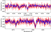 |
Fig. 8. Selected regions of the reconstructed spectrum B for the detection of the secondary component in HD 96118: Si II lines (top) and Fe II and Mg II lines (bottom). Original data are plotted in red, and a smoothed version is plotted in blue for better visibility. |
5.5. HD 127124
is a long-period, eccentric binary with a K0V-type primary with magnitude V = 9.53, effective temperature Teff = 5030 K, age 5.36 Gyr, and mass M = 0.804 ± 0.023 M⊙ (Gomes da Silva et al. 2021).
Due to the poor orbital coverage, the orbital period cannot be determined from the RV curve, and only a lower limit of about 9000 d can be established (see Fig. A.5). The residuals become significantly higher for periods below 9000 d. Feng et al. (2022) claimed to have found evidence of a substellar companion of 0.106 M⊙ and reported an orbital period of P = 16.957 yr and an RV half-amplitude of  km s−1. However, they used only the spectroscopic observations earlier than JD = 2 457 150 (the flat part of the RV curve), and their parameters are incompatible with the later data. With the observational data currently available, the resulting highly eccentric orbit has a much larger amplitude, giving a minimum secondary mass of 0.24 M⊙.
Using the task vgrid we searched for the best solution in the range of systemic velocities γ from 11.0 to 12.8 km s−1. We found a maximum correlation function for γ = 11.4 km s−1, q = 0.34, and Teff, B = 4600 K for log g = +2.5 (Fig. B.5). From our mass ratio and the primary mass estimated by Gomes da Silva et al. (2021), we obtained a mass of MB = 0.274 ± 0.008 M⊙ for the secondary star. The temperature of the template with the best correlation (4600 K) is significantly higher than the expected temperature for this mass.
For a grid of possible periods, we fit the orbit and derived the projected mass MAsin3i. The condition that this parameter is smaller than the estimated primary mass (0.804 M⊙) imposes an upper limit of 11 000 d on the period, since solutions with very long periods require high values of eccentricity and amplitude. The orbital period is thus constrained to a rather narrow range: 9000 d < P < 11 000 d.
5.6. HD 160346
(GJ688) is a bright (V = 6.53 mag) K3 V star classified as SB1. Casagrande et al. (2011) estimated an effective temperature of Teff, A = 4841 K. Katoh et al. (2013) estimated the primary mass from the temperature and determined the orbital parameters, obtaining: MA = 0.75 ± 0.02 M⊙, P = 83.72696 ± 0.00084 , MB, min = 0.105 ± 0.001 M⊙, and qmin = 0.14 ± 0.01. In an independent study with CORAVEL (COrrelation RAdial VELocities), Halbwachs et al. (2018) redetermined the orbital parameters and found P = 83.714 ± 0.012 d, KA = 5.644 km s−1, and γ = 21.680 km s−1. Gomes da Silva et al. (2021) estimated a primary mass of 0.795 ± 0.026 M⊙.
Figure A.6 shows our RV curve fit and Fig. B.6 the results of the BiSpeD analysis. We found a mass ratio q = 0.49 and a secondary star temperature Teff, B = 3700 K for log g = +2.0. The secondary mass is MB = 0.39 ± 0.012 M⊙, according to our mass ratio and the primary mass estimated by Gomes da Silva et al. (2021).
5.7. HD 178445
is a V = 9.342 magnitude, K6.5 V star (Gray et al. 2006). We obtained the following orbital parameters: period P = 62.820 d, RV semi-amplitude KA = 15.51 km s−1, and eccentricity e = 0.374 (see Fig. A.7). The BiSpeD analysis yielded a mass ratio q = 0.37 and an effective temperature of the secondary star Teff, B = 3800 K for log g = +2.5 (Fig. B.7). Assuming a mass of 0.68 M⊙ for the primary, the secondary mass results 0.25 M⊙, making this object one of the lowest-mass stars in our sample. The secondary temperature is expected to be on the order of 3250 K, significantly lower than that of the best template selected by find2c.
5.8. HD 219630
is a V = 10.4 star of spectral type K6+ V (k) (Gray et al. 2006), with a primary component mass MA = 0.707 ± 0.013 M⊙ (Mann et al. 2015).
The RV measurements show a clear variation with an amplitude of about 7 km s−1, but the time span of the observations does not cover a single orbital cycle, so the period cannot be precisely determined. We obtained the best fit for P = 6521 d, KA = 3.74 km s−1, γ = −2.16 km s−1, and e = 0.383 (Fig. A.8). To confirm the systemic RV of the fit, we run the vgrid task with γmin = −4.2 km s−1 and γmax = 0 km s−1 finding the best solution for γ = −2.2 km s−1, q = 0.41, and Teff, B = 3700 K for the template series of log g = +2.0 (see Fig. B.8). From the mass estimate of Mann et al. (2015) we get a companion mass of 0.29 M⊙.
5.9. PM J21214-6655
is a main-sequence star with spectral type M0 (Schneider et al. 2019) and magnitude V = 10.595. Reiners & Zechmeister (2020) have estimated the stellar mass to be 0.61 M⊙. The RV curve shows that it is a long-period eccentric binary (Fig. A.9). From the BiSpeD analysis we found a mass ratio q = 0.63 and an effective temperature for the secondary component of Teff, B = 3800 K for log g = +2.5 (see Fig. B.9). The secondary companion mass would then be 0.38 M⊙.
5.10. PX Virginis
(HD 113449) is an SB1 (Griffin 2010) of magnitude V = 7.679, classified as BY Dra-type by Samus’ et al. (2017). A more detailed analysis of this object is presented in Sect. 6 of Paper I. We have shown there that the secondary flux and the S/N are high enough that the spectral morphology is clearly visible in the reconstructed spectrum of the secondary companion, and that its RV can be measured in single spectra by spectral disentangling. In Figs. A.10 and B.10 we show for this object the results obtained using the standard procedure adopted in this paper, including the use of templates with surface gravity values different from those of the main-sequence stars. The obtained value for the mass ratio is the same (q = 0.59), but a slightly lower temperature is found (Teff, B = 3900 K for log g = +3.5), which is more consistent with the secondary spectral morphology (see Fig. 13 in Paper I).
5.11. Ross 193
(FR Aquarii) is a M3 dwarf star of V = 11.916 magnitude (Stephenson 1986) with Teff = 3089 K (Kuznetsov et al. 2019). This star was classified as an eruptive variable (Samus’ et al. 2017) and reported as an astrometric binary with a white dwarf companion (McCook & Sion 1999; Mason et al. 2001; Holberg et al. 2008). We obtained a period P = 23.99 d, RV semi-amplitude KA = 4.51 km s−1 and eccentricity e = 0.461 (Fig. A.11). The BiSpeD analysis gave a mass ratio q = 0.67 and an effective temperature for the secondary component of Teff, B = 3800 K, for log g = +4.5 (Fig. B.11). The mass of the secondary star would be only 0.23 M⊙.
5.12. Wolf 414
is a low-mass main-sequence star of magnitude V = 12.047 and spectral type M4V that has been reported as a double by Lamman et al. (2020), with a visual companion 1.6 mag fainter, at 0.29 arcsec. Since the temporal sampling of the HARPS velocity dataset is poor (only 6 epochs), we measure a publicly available FEROS (Fibre-fed Extended Range Optical Spectrograph) spectrum for this object to allow period identification. The resulting orbital parameters are: period P = 4419.7 d, semi-amplitude KA = 3.46 km s−1, systemic velocity γ = −7.34 km s−1 and eccentricity e = 0.315 (Fig. B.12). The resulting secondary detection function has a broad peak at mass ratio q = 0.44 and effective temperature Teff, B = 4200 K for log g = +3.0 (Fig. B.12). This binary has been astrometrically studied and the total mass of the system has been calculated to be 0.514 ± 0.011 M⊙ (Mann et al. 2019). From this value and our mass ratio, the masses of the components are MA = 0.357 ± 0.011 M⊙ and MB = 0.157 ± 0.008 M⊙, which agree with the minimum secondary mass and the primary mass estimated from the HR diagram (see Table 3). The secondary of this system is therefore the smallest of all the stars detected in this work.
6. Conclusions
We present BiSpeD, a PYTHON repository containing a function called find2c that implements the method introduced in Paper I for detecting a faint companion in a spectroscopic binary star. Specifically, the goal is to calculate the mass ratio between the companions and to estimate the secondary effective temperature in systems classified as SB1s.
As a preliminary analysis to test the performance of the scripts, we modeled synthetic binary observations using single star spectra and synthetic templates. Applying the code to synthetic observations helped us optimize the execution of the scripts and find the limitations of our method. We performed tests on several synthetic binary systems consisting of main-sequence stars of spectral types F–M. From synthetic observational datasets of a few tens of spectra with a S/N of about 100, it was possible to detect the faint companion in pairs with a luminosity ratio of LB/LA ∼ 0.003 (i.e., a magnitude difference of about 6 mag).
To explore the applicability of the method to the detection of low-mass stars, we applied the find2c task to a list of 41 SB1 candidates selected from the HARPS database according to the following criteria: spectral type between K0 and M7, ΔRV > 1 km s−1, and number of observations N ≥ 8. We found solutions for 12 systems in the list: CD-35 15144, HD 4457, HD 24706, HD 96118, HD 127124, HD 160346, HD 178445, HD 219630, PM J21214-6655, Ross 193, PX Vir (described in more detail in Paper I), and Wolf 414. Using the primary mass estimates, we inferred the secondary masses, finding values between 0.16 and 0.49 M⊙ for the ten binaries with main-sequence primaries. In three cases where the available observations were insufficient to determine the orbital period, we added the center-of-mass velocity as an additional free parameter using the vgrid task. This was the case for Wolf 414, which is the binary system with the lowest secondary mass (0.16 M⊙) detected in the present work. This system has an astrometric orbit from which absolute masses could be derived. A few stars with evolved primaries were included in our sample, and for two of them we detected the secondary signal: HD 24706 with a K2III primary and a solar-type main-sequence secondary, and HD 96118 with a K3III primary and a B8-B9 main-sequence secondary of about 3 M⊙.
We find that although the mass ratio determination seems to be robust, the temperature estimation is more sensitive to the particular choice of the template grid, which is not unreasonable since the mass ratio is related to spectral shifts while the temperature depends on the spectral morphology. In the general strategy adopted in the present work, we included a large template grid with log g as an additional free parameter in order to find a reference spectrum that maximizes the secondary signal even if the gravity values are not as expected according to the luminosity class. For nine objects on the sample list, the mass ratios for different grids with log g between +2.0 and +5.0 differ by Δq = 0.01, but the effective temperatures differ by up to ΔTeff = 400 K. The only two objects for which the mass ratio depends on log g are Ross 193 and Wolf 414, but the secondary mass in each case is in agreement with the expected mass for main-sequence stars (in particular, for Ross 193 we find log g = +4.5).
Thus, it is clear that the present template grid overestimates the temperatures obtained for the cooler objects, since no template below 3700 K was selected in any case. Differences in chemical abundances, rotation, spectrum filtering (the low-frequency balance between the primary and secondary during the disentangling process), and deficiencies in the atmosphere model could contribute to this, but an analysis of these effects is beyond the scope of this paper. It should be noted, however, that this does not undermine the secondary detection and mass ratio determination, which are the main goals of the program.
For 29 stars in our sample we did not obtain positive detections. Three stars had broadly lined spectra, and in two cases the RV measurements were inconsistent with a spectroscopic orbit. For 13 stars, the observations had insufficient orbital phase coverage (all observations concentrated in two or three phases). For the remaining 11 objects we fitted a Keplerian orbital model, but the find2c task did not find a solution that met the detection criterion defined in Sect. 3 of Paper I (a cross-correlation function with S/N ≥10). To illustrate these cases of non-detection due to low S/N, we have shown the results for the star CD-45 7872, for which a possible solution was found at q = 0.25 and Teff, B = 3300 K. Although the solution seems to be consistent with respect to q and Teff, B, the correlation peak is only 4.44 times the noise, σ. Some of these cases may become positive if additional spectroscopic observations are included.
Data availability
The BiSpeD repository is available on GitHub, at http://github.com/israelmarti/BiSpeD. The data underlying this article will be made available upon reasonable request to the corresponding author.
The ssynth package is available on GitHub http://github.com/israelmarti/ssynth
www.pas.rochester.edu/~emamajek/EEM_dwarf_UBVIJHK_colors_Teff.txt, accessed 2019-3-22.
Acknowledgments
Based on observations collected at the European Southern Observatory under programs IDs: 094.A-9029, 0100.C-0097, 0101.C-0379, 0102.C-0558, 0103.C-0432, 0106.C-1067, 0108.C-0879, 072.C-0096, 072.C-0488, 073.D-0038, 074.C-0364, 074.D-0131, 075.C-0202, 075.C-0332, 075.D-0194, 076.C-0010, 076.D-0130, 077.C-0012, 077.C-0364, 077.D-0085, 078.C-0044, 078.C-0751, 078.D-0071, 078.D-0245, 079.C-0046, 079.C-0657, 079.D-0075, 080.D-0086, 081.C-0802, 081.D-0065, 082.C-0357, 082.C-0427, 082.C-0718, 083.C-0794, 085.C-0019, 087.C-0831, 089.C-0732, 090.C-0421, 091.C-0034, 092.C-0721, 093.C-0409, 095.C-0551, 096.C-0460, 097.C-0864, 098.C-0366, 099.C-0458, 106.21R4.001, 108.222V.001, 1102.C-0339, 180.C-0886, 183.C-0437, 183.C-0972, 192.C-0224, 192.C-0852, and 196.C-1006.
References
- Andrae, R., Fouesneau, M., Creevey, O., et al. 2018, A&A, 616, A8 [NASA ADS] [CrossRef] [EDP Sciences] [Google Scholar]
- Anglada-Escudé, G., & Butler, R. P. 2012, ApJS, 200, 15 [Google Scholar]
- Bahcall, J. N., & Soneira, R. M. 1980, ApJS, 44, 73 [NASA ADS] [CrossRef] [Google Scholar]
- Benedict, G. F., Henry, T. J., Franz, O. G., et al. 2016, AJ, 152, 141 [Google Scholar]
- Casagrande, L., Schönrich, R., Asplund, M., et al. 2011, A&A, 530, A138 [NASA ADS] [CrossRef] [EDP Sciences] [Google Scholar]
- Chabrier, G., & Baraffe, I. 1997, A&A, 327, 1039 [NASA ADS] [Google Scholar]
- Chen, Y., Girardi, L., Bressan, A., et al. 2014, MNRAS, 444, 2525 [Google Scholar]
- Choi, J., Dotter, A., Conroy, C., et al. 2016, ApJ, 823, 102 [Google Scholar]
- Coelho, P., Barbuy, B., Meléndez, J., Schiavon, R. P., & Castilho, B. V. 2005, A&A, 443, 735 [NASA ADS] [CrossRef] [EDP Sciences] [Google Scholar]
- Danielski, C., Babusiaux, C., Ruiz-Dern, L., Sartoretti, P., & Arenou, F. 2018, A&A, 614, A19 [NASA ADS] [CrossRef] [EDP Sciences] [Google Scholar]
- Davis, Y. T., Triaud, A. H. M. J., Freckelton, A. V., et al. 2024, MNRAS, 530, 2565 [Google Scholar]
- Delfosse, X., Forveille, T., Ségransan, D., et al. 2000, A&A, 364, 217 [NASA ADS] [Google Scholar]
- Delisle, J. B., Ségransan, D., Buchschacher, N., & Alesina, F. 2016, A&A, 590, A134 [NASA ADS] [CrossRef] [EDP Sciences] [Google Scholar]
- Feng, F., Butler, R. P., Vogt, S. S., et al. 2022, ApJS, 262, 21 [NASA ADS] [CrossRef] [Google Scholar]
- Gaia Collaboration (Vallenari, A., et al.) 2023, A&A, 674, A1 [NASA ADS] [CrossRef] [EDP Sciences] [Google Scholar]
- Gaidos, E., Mann, A. W., Lépine, S., et al. 2014, MNRAS, 443, 2561 [Google Scholar]
- Gomes da Silva, J., Santos, N. C., Adibekyan, V., et al. 2021, A&A, 646, A77 [NASA ADS] [CrossRef] [EDP Sciences] [Google Scholar]
- González, J. F., & Levato, H. 2006, A&A, 448, 283 [NASA ADS] [CrossRef] [EDP Sciences] [Google Scholar]
- González, J. F., Martínez, C. I., & Alejo, A. D. 2024, A&A, 690, A124 [NASA ADS] [CrossRef] [EDP Sciences] [Google Scholar]
- Gray, R. O., Corbally, C. J., Garrison, R. F., et al. 2006, AJ, 132, 161 [Google Scholar]
- Griffin, R. F. 2010, Observatory, 130, 125 [Google Scholar]
- Halbwachs, J. L., Mayor, M., & Udry, S. 2018, A&A, 619, A81 [NASA ADS] [CrossRef] [EDP Sciences] [Google Scholar]
- Holberg, J. B., Sion, E. M., Oswalt, T., et al. 2008, AJ, 135, 1225 [NASA ADS] [CrossRef] [Google Scholar]
- Houk, N. 1978, Michigan Catalogue of Two-dimensional Spectral Types for the HD Stars (Department of Astronomy, University of Michigan) [Google Scholar]
- Houk, N., & Cowley, A. P. 1975, University of Michigan Catalogue of Two-dimensional Spectral Types for the HD Stars. Volume I. Declinations–90_to–53_f0 (Department of Astronomy, University of Michigan) [Google Scholar]
- Husser, T. O., Wende-von Berg, S., Dreizler, S., et al. 2013, A&A, 553, A6 [NASA ADS] [CrossRef] [EDP Sciences] [Google Scholar]
- Katoh, N., Itoh, Y., Toyota, E., & Sato, B. 2013, AJ, 145, 41 [Google Scholar]
- Kervella, P., Arenou, F., & Thévenin, F. 2022, A&A, 657, A7 [NASA ADS] [CrossRef] [EDP Sciences] [Google Scholar]
- Kirkpatrick, J. D., Marocco, F., Gelino, C. R., et al. 2024, ApJS, 271, 55 [NASA ADS] [CrossRef] [Google Scholar]
- Koen, C., Kilkenny, D., van Wyk, F., & Marang, F. 2010, MNRAS, 403, 1949 [Google Scholar]
- Kuznetsov, M. K., del Burgo, C., Pavlenko, Y. V., & Frith, J. 2019, ApJ, 878, 134 [Google Scholar]
- Lamman, C., Baranec, C., Berta-Thompson, Z. K., et al. 2020, AJ, 159, 139 [Google Scholar]
- Li, J., Liu, C., Zhang, Z.-Y., et al. 2023, Nature, 613, 460 [NASA ADS] [CrossRef] [Google Scholar]
- Liu, Y. J., Zhao, G., Shi, J. R., Pietrzyński, G., & Gieren, W. 2007, MNRAS, 382, 553 [NASA ADS] [CrossRef] [Google Scholar]
- López-Morales, M. 2007, ApJ, 660, 732 [Google Scholar]
- Mann, R. K., Andrews, S. M., Eisner, J. A., et al. 2015, ApJ, 802, 77 [Google Scholar]
- Mann, A. W., Dupuy, T., Kraus, A. L., et al. 2019, ApJ, 871, 63 [Google Scholar]
- Marshall, D. J., Robin, A. C., Reylé, C., Schultheis, M., & Picaud, S. 2006, A&A, 453, 635 [NASA ADS] [CrossRef] [EDP Sciences] [Google Scholar]
- Mason, B. D., Wycoff, G. L., Hartkopf, W. I., Douglass, G. G., & Worley, C. E. 2001, AJ, 122, 3466 [Google Scholar]
- Mayor, M., Pepe, F., Queloz, D., et al. 2003, Messenger, 114, 20 [Google Scholar]
- McCook, G. P., & Sion, E. M. 1999, ApJS, 121, 1 [Google Scholar]
- Mermilliod, J. C., Andersen, J., Latham, D. W., & Mayor, M. 2007, A&A, 473, 829 [NASA ADS] [CrossRef] [EDP Sciences] [Google Scholar]
- Morales, J. C., Ribas, I., Giménez, Á., & Baroch, D. 2022, Galaxies, 10, 98 [NASA ADS] [CrossRef] [Google Scholar]
- Nguyen, C. T., Costa, G., Girardi, L., et al. 2022, A&A, 665, A126 [NASA ADS] [CrossRef] [EDP Sciences] [Google Scholar]
- Paxton, B., Bildsten, L., Dotter, A., et al. 2011, ApJS, 192, 3 [Google Scholar]
- Pecaut, M. J., & Mamajek, E. E. 2013, ApJS, 208, 9 [Google Scholar]
- Pepe, F., Mayor, M., Rupprecht, G., et al. 2002, Messenger, 110, 9 [Google Scholar]
- Pourbaix, D., Tokovinin, A. A., Batten, A. H., et al. 2004, A&A, 424, 727 [NASA ADS] [CrossRef] [EDP Sciences] [Google Scholar]
- Reiners, A., & Zechmeister, M. 2020, ApJS, 247, 11 [CrossRef] [Google Scholar]
- Ribas, I. 2006, Ap&SS, 304, 89 [Google Scholar]
- Samus’, N. N., Kazarovets, E. V., Durlevich, O. V., Kireeva, N. N., & Pastukhova, E. N. 2017, Astron. Rep., 61, 80 [Google Scholar]
- Scalo, J. M. 1986, Fund. Cosmic Phys., 11, 1 [NASA ADS] [EDP Sciences] [Google Scholar]
- Schneider, A. C., Shkolnik, E. L., Allers, K. N., et al. 2019, AJ, 157, 234 [Google Scholar]
- Serenelli, A., Weiss, A., Aerts, C., et al. 2021, A&ARv, 29, 4 [Google Scholar]
- Sneden, C. 1973, ApJ, 184, 839 [Google Scholar]
- Soubiran, C., Brouillet, N., & Casamiquela, L. 2022, A&A, 663, A4 [NASA ADS] [CrossRef] [EDP Sciences] [Google Scholar]
- Sousa, S. G., Santos, N. C., Israelian, G., Mayor, M., & Udry, S. 2011, A&A, 533, A141 [NASA ADS] [CrossRef] [EDP Sciences] [Google Scholar]
- Stephenson, C. B. 1986, AJ, 92, 139 [NASA ADS] [CrossRef] [Google Scholar]
- Swayne, M. I., Maxted, P. F. L., Triaud, A. H. M. J., et al. 2024, MNRAS, 528, 5703 [NASA ADS] [CrossRef] [Google Scholar]
- Tonry, J., & Davis, M. 1979, AJ, 84, 1511 [Google Scholar]
- Triaud, A. H. M. J., Hebb, L., Anderson, D. R., et al. 2013, A&A, 549, A18 [NASA ADS] [CrossRef] [EDP Sciences] [Google Scholar]
- Trifonov, T., Tal-Or, L., Zechmeister, M., et al. 2020, A&A, 636, A74 [NASA ADS] [CrossRef] [EDP Sciences] [Google Scholar]
- Tsantaki, M., Delgado-Mena, E., Bossini, D., et al. 2023, A&A, 674, A157 [NASA ADS] [CrossRef] [EDP Sciences] [Google Scholar]
- Tuomi, M., Jones, H. R. A., Barnes, J. R., Anglada-Escudé, G., & Jenkins, J. S. 2014, MNRAS, 441, 1545 [Google Scholar]
- Upgren, A. R., Grossenbacher, R., Penhallow, W. S., MacConnell, D. J., & Frye, R. L. 1972, AJ, 77, 486 [NASA ADS] [CrossRef] [Google Scholar]
- Wang, X., Xia, F., & Fu, Y. 2023, PASJ, 75, 368 [NASA ADS] [CrossRef] [Google Scholar]
- Wildi, F., Pepe, F., Chazelas, B., Lo Curto, G., & Lovis, C. 2010, in Ground-based and Airborne Instrumentation for Astronomy III, eds. I. S. McLean, S. K. Ramsay, & H. Takami, Society of Photo-Optical Instrumentation Engineers (SPIE) Conference Series, 7735, 77354X [NASA ADS] [Google Scholar]
- Zechmeister, M., Kürster, M., & Endl, M. 2009, A&A, 505, 859 [NASA ADS] [CrossRef] [EDP Sciences] [Google Scholar]
Appendix A: Summary of orbital parameters
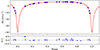 |
Fig. A.1. Phase curve of CD-35 15144 for the orbital period P = 172.532 d. The RV measurements are shown as blue dots. The bottom panel shows the residuals of the orbital fit. For some points, the error bars are smaller than the size of the marker. |
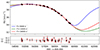 |
Fig. A.2. RV as a function of time (HJD−2, 400 000) of HD 4457 for three different orbital periods: 18000 d (red), 14000 d (green), and 9000 d (blue). The RV measurements are shown as black dots. The bottom panel shows the residuals of the orbital fit for P = 18000 d. |
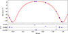 |
Fig. A.3. Phase curve of HD 24706 for the orbital period P = 1493 d. The RV measurements are marked with blue dots. The bottom panel shows the residuals of the orbital fit. The error bars are smaller than the size of the markers. |
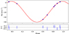 |
Fig. A.4. Phase curve of HD 96118 for orbital period P = 336.660 d. The RV measurements are shown as blue dots. The bottom panel shows the residuals of the orbital fit. |
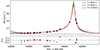 |
Fig. A.5. RV as a function of time (HJD−2 400 000) of HD 127124 for orbital periods 8000 d, 9000 d, and 11000 d. The RV measurements are shown as black dots. The bottom panel shows the residuals of the orbital fits. The error bars have been disabled to see the scatter for different fits. |
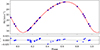 |
Fig. A.6. Phase curve of HD 160346 for the orbital period P = 83.728 d. The RV measurements are marked with blue dots. The bottom panel shows the residuals of the orbital fit. The error bars are smaller than the size of the markers. |
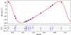 |
Fig. A.7. Phase curve of HD 178445 for the orbital period P = 62.820 d. The RV measurements are marked with blue dots. The bottom panel shows the residuals of the orbital fit. |
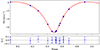 |
Fig. A.8. Phase curve of HD 219630 for orbital period P = 6521 d. The RV measurements are marked with blue dots. The bottom panel shows the residuals of the orbital fit. |
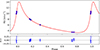 |
Fig. A.9. Phase curve of PM J21214-6655 for orbital period P = 549 d. The RV measurements are marked with blue dots. The bottom panel shows the residuals of the orbital fit. |
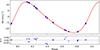 |
Fig. A.10. Phase curve of PX Vir for the orbital period P = 216.483 d. The RV measurements are marked with blue dots. The bottom panel shows the residuals of the orbital fit. The error bars are smaller than the size of the markers. |
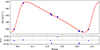 |
Fig. A.11. Phase curve of Ross 193 for the orbital period P = 23.99 d. The RV measurements are shown as blue dots. The bottom panel shows the residuals of the orbital fit. Error bars are smaller than the size of the marker.. |
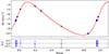 |
Fig. A.12. Phase curve of Wolf 414 for the orbital period P = 4419.7 d. The RV measurements are marked as blue (HARPS) and green (FEROS) points. The bottom panel shows the residuals of the orbital fit. |
Appendix B: Summary of BiSpeD detections
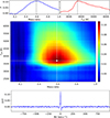 |
Fig. B.1. Output of find2c for CD-35 15144. Top: SSF value as a function of mass ratio, q (left) and effective temperature for the secondary companion, Teff, B (right). Middle: 2D density plot for ℱ; the best solution corresponds to q = 0.59 and Teff, B = 3700 K for log g = +2.0. Bottom: Cross-correlation function between the resulting secondary spectrum, Bq = 0.59, and a template of 3700 K. |
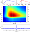 |
Fig. B.2. Output of find2c for HD 4457. Top: SSF value as a function of the mass ratio, q (left) and the effective temperature for the secondary companion, Teff, B (right). Middle: 2D density plot for ℱ;, the best solution corresponds to q = 0.46 and Teff, B = 3800 K for log g = +2.5. Bottom: Cross-correlation function between the resulting secondary spectrum, Bq = 0.46, and a template of 3800 K. |
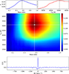 |
Fig. B.3. Output of find2c for HD 24706. Top: SSF value as a function of the mass ratio, q (left) and the effective temperature for the secondary companion, Teff, B (right). Middle: 2D density plot for ℱ; the best solution corresponds to q = 0.57 and Teff, B = 5100 K for log g = +3.5. Bottom: Cross-correlation function between the resulting secondary spectrum, Bq = 0.57, and a template of 5100 K. |
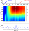 |
Fig. B.4. Output of find2c for HD 96118. Top: SSF value as a function of the mass ratio, q (left) and the effective temperature for the secondary companion, Teff, B (right). Middle: 2D density plot for ℱ, the best solution corresponds to q = 0.6 and Teff, B = 11750 K. Bottom: Cross-correlation function between the resulting secondary spectrum, Bq = 0.6, and a template at 11750 K. |
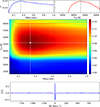 |
Fig. B.5. Output of find2c for HD 127124. Top: SSF value as a function of the mass ratio, q (left) and the effective temperature for the secondary companion, Teff, B (right). Middle: 2D density plot for ℱ; the best solution corresponds to q = 0.34 and Teff, B = 4600 K for log g = +2.0. Bottom: Cross-correlation function between the resulting secondary spectrum, Bq = 0.34, and a template of 4600 K. |
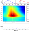 |
Fig. B.6. Output of find2c for HD 160346. Top: SSF value as a function of the mass ratio, q (left) and the effective temperature for the secondary companion, Teff, B (right). Middle: 2D density plot for ℱ; the best solution corresponds to q = 0.49 and Teff, B = 3700 K for log g = +2.0. Bottom: Cross-correlation function between the resulting secondary spectrum, Bq = 0.49, and a template of 3700 K. |
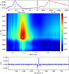 |
Fig. B.7. Output of find2c for HD 178445. Top: SSF value as a function of the mass ratio, q (left) and the effective temperature for the secondary companion, Teff, B (right). Middle: 2D density plot for ℱ; the best solution corresponds to q = 0.37 and Teff, B = 3800 K for log g = +2.5. Bottom: Cross-correlation function between the resulting secondary spectrum, Bq = 0.37, and a template of 3800 K. |
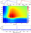 |
Fig. B.8. Output of find2c for HD 219630. Top: SSF value as a function of the mass ratio, q (left) and the effective temperature for the secondary companion, Teff, B (right). Middle: 2D density plot for ℱ; the best solution corresponds to q = 0.41 and Teff, B = 3700 K for log g = +2.0. Bottom: Cross-correlation function between the resulting secondary spectrum, Bq = 0.41, and a template of 3700 K.. |
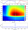 |
Fig. B.9. Output of find2c for PM J21214-6655. Top: SSF value as a function of the mass ratio, q (left) and the effective temperature for the secondary companion, Teff, B (right). Middle: 2D density plot for ℱ; the best solution corresponds to q = 0.63 and Teff, B = 3800 K for log g = +2.5. Bottom: Cross-correlation function between the resulting secondary spectrum, Bq = 0.63, and a template of 3800 K. |
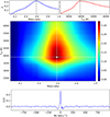 |
Fig. B.10. Output of find2c for PX Vir. Top: SSF value as a function of mass ratio, q (left) and effective temperature for the secondary companion, Teff, B (right). Middle: 2D density plot for ℱ; the best solution corresponds to q = 0.59 and Teff, B = 3900 K for log g = +3.5. Bottom: Cross-correlation function between the resulting secondary spectrum, Bq = 0.59, and a template of 3900 K. |
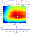 |
Fig. B.11. Output of find2c for Ross 193. Top: SSF value as a function of the mass ratio, q (left) and the effective temperature for the secondary companion,Teff, B (right). Middle: 2D density plot for ℱ; the best solution corresponds to q = 0.67 and Teff, B = 3800 K for log g = +4.5. Bottom: Cross-correlation function between the resulting secondary spectrum, Bq = 0.67, and a template of 3800 K. |
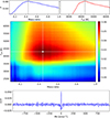 |
Fig. B.12. Output of find2c for Wolf 414. Top: SSF value as a function of the mass ratio, q (left) and the effective temperature for the secondary companion, Teff, B (right). Middle: 2D density plot for ℱ; the best solution corresponds to q = 0.44 and Teff, B = 4200 K for log g = +3.0. Bottom: Cross-correlation function between the resulting secondary spectrum, Bq = 0.44, and a template of 4200 K. |
All Tables
All Figures
|
Fig. 1. Example of one of the synthetic spectra associated with the modeled binary (red) and a spectrum template of the effective temperature Teff = 4400 K (blue). The spectral features correspond to the primary component; the spectral features of the secondary companions cannot be seen due to the noise level added in the modeled synthetic binary. |
| In the text | |
|
Fig. 2. GUI 3D standard output of the find2c analysis over the synthetic example. Top: 3D density plot for the SSF. Bottom left: Mass ratio cross section for the best effective temperature peak. Bottom right: Effective temperature cross section for the best mass ratio. For the maximum ℱ peak the values are q = 0.32 and Teff, B = 3300 K (marked by dotted gray lines). |
| In the text | |
|
Fig. 3. BiSpeD analysis of the synthetic example correlated with different template grids; the colors correspond to the log g used. Left: Mass ratio cross section for the best effective temperature peak. Right: Effective temperature cross section for the best mass ratio. |
| In the text | |
|
Fig. 4. 3D density plot for ℱ(q, Teff) for increasing values of the systemic velocities from γmin = −2.5 km s−1 on the top left to γmax = 3.0 km s−1 on the bottom right, in steps of 0.5 km s−1. The best solution is γ = 0 km s−1. |
| In the text | |
|
Fig. 5. HR diagram of a sample of stars. Stars are colored according to their luminosity class: V (blue), IV (orange), III (red), and unclassified (green). |
| In the text | |
|
Fig. 6. Phase curve of CD-45 7872 for orbital period P = 587.179 d. The RV measurements are shown as blue dots. The bottom panel shows the residuals of the orbital fit. |
| In the text | |
|
Fig. 7. Example of a non-detection case for the star CD-45 7872. Top: Cross sections of the SSF as a function of the mass ratio, q (left) and the effective temperature of the secondary companion, Teff, B (right). Middle: 2D density plot for ℱ; the best solution corresponds to q = 0.25 and Teff, B = 3300 K. Bottom: Cross-correlation function between the best secondary spectrum, Bq = 0.25, and a template of 3300 K. |
| In the text | |
|
Fig. 8. Selected regions of the reconstructed spectrum B for the detection of the secondary component in HD 96118: Si II lines (top) and Fe II and Mg II lines (bottom). Original data are plotted in red, and a smoothed version is plotted in blue for better visibility. |
| In the text | |
|
Fig. A.1. Phase curve of CD-35 15144 for the orbital period P = 172.532 d. The RV measurements are shown as blue dots. The bottom panel shows the residuals of the orbital fit. For some points, the error bars are smaller than the size of the marker. |
| In the text | |
|
Fig. A.2. RV as a function of time (HJD−2, 400 000) of HD 4457 for three different orbital periods: 18000 d (red), 14000 d (green), and 9000 d (blue). The RV measurements are shown as black dots. The bottom panel shows the residuals of the orbital fit for P = 18000 d. |
| In the text | |
|
Fig. A.3. Phase curve of HD 24706 for the orbital period P = 1493 d. The RV measurements are marked with blue dots. The bottom panel shows the residuals of the orbital fit. The error bars are smaller than the size of the markers. |
| In the text | |
|
Fig. A.4. Phase curve of HD 96118 for orbital period P = 336.660 d. The RV measurements are shown as blue dots. The bottom panel shows the residuals of the orbital fit. |
| In the text | |
|
Fig. A.5. RV as a function of time (HJD−2 400 000) of HD 127124 for orbital periods 8000 d, 9000 d, and 11000 d. The RV measurements are shown as black dots. The bottom panel shows the residuals of the orbital fits. The error bars have been disabled to see the scatter for different fits. |
| In the text | |
|
Fig. A.6. Phase curve of HD 160346 for the orbital period P = 83.728 d. The RV measurements are marked with blue dots. The bottom panel shows the residuals of the orbital fit. The error bars are smaller than the size of the markers. |
| In the text | |
|
Fig. A.7. Phase curve of HD 178445 for the orbital period P = 62.820 d. The RV measurements are marked with blue dots. The bottom panel shows the residuals of the orbital fit. |
| In the text | |
|
Fig. A.8. Phase curve of HD 219630 for orbital period P = 6521 d. The RV measurements are marked with blue dots. The bottom panel shows the residuals of the orbital fit. |
| In the text | |
|
Fig. A.9. Phase curve of PM J21214-6655 for orbital period P = 549 d. The RV measurements are marked with blue dots. The bottom panel shows the residuals of the orbital fit. |
| In the text | |
|
Fig. A.10. Phase curve of PX Vir for the orbital period P = 216.483 d. The RV measurements are marked with blue dots. The bottom panel shows the residuals of the orbital fit. The error bars are smaller than the size of the markers. |
| In the text | |
|
Fig. A.11. Phase curve of Ross 193 for the orbital period P = 23.99 d. The RV measurements are shown as blue dots. The bottom panel shows the residuals of the orbital fit. Error bars are smaller than the size of the marker.. |
| In the text | |
|
Fig. A.12. Phase curve of Wolf 414 for the orbital period P = 4419.7 d. The RV measurements are marked as blue (HARPS) and green (FEROS) points. The bottom panel shows the residuals of the orbital fit. |
| In the text | |
|
Fig. B.1. Output of find2c for CD-35 15144. Top: SSF value as a function of mass ratio, q (left) and effective temperature for the secondary companion, Teff, B (right). Middle: 2D density plot for ℱ; the best solution corresponds to q = 0.59 and Teff, B = 3700 K for log g = +2.0. Bottom: Cross-correlation function between the resulting secondary spectrum, Bq = 0.59, and a template of 3700 K. |
| In the text | |
|
Fig. B.2. Output of find2c for HD 4457. Top: SSF value as a function of the mass ratio, q (left) and the effective temperature for the secondary companion, Teff, B (right). Middle: 2D density plot for ℱ;, the best solution corresponds to q = 0.46 and Teff, B = 3800 K for log g = +2.5. Bottom: Cross-correlation function between the resulting secondary spectrum, Bq = 0.46, and a template of 3800 K. |
| In the text | |
|
Fig. B.3. Output of find2c for HD 24706. Top: SSF value as a function of the mass ratio, q (left) and the effective temperature for the secondary companion, Teff, B (right). Middle: 2D density plot for ℱ; the best solution corresponds to q = 0.57 and Teff, B = 5100 K for log g = +3.5. Bottom: Cross-correlation function between the resulting secondary spectrum, Bq = 0.57, and a template of 5100 K. |
| In the text | |
|
Fig. B.4. Output of find2c for HD 96118. Top: SSF value as a function of the mass ratio, q (left) and the effective temperature for the secondary companion, Teff, B (right). Middle: 2D density plot for ℱ, the best solution corresponds to q = 0.6 and Teff, B = 11750 K. Bottom: Cross-correlation function between the resulting secondary spectrum, Bq = 0.6, and a template at 11750 K. |
| In the text | |
|
Fig. B.5. Output of find2c for HD 127124. Top: SSF value as a function of the mass ratio, q (left) and the effective temperature for the secondary companion, Teff, B (right). Middle: 2D density plot for ℱ; the best solution corresponds to q = 0.34 and Teff, B = 4600 K for log g = +2.0. Bottom: Cross-correlation function between the resulting secondary spectrum, Bq = 0.34, and a template of 4600 K. |
| In the text | |
|
Fig. B.6. Output of find2c for HD 160346. Top: SSF value as a function of the mass ratio, q (left) and the effective temperature for the secondary companion, Teff, B (right). Middle: 2D density plot for ℱ; the best solution corresponds to q = 0.49 and Teff, B = 3700 K for log g = +2.0. Bottom: Cross-correlation function between the resulting secondary spectrum, Bq = 0.49, and a template of 3700 K. |
| In the text | |
|
Fig. B.7. Output of find2c for HD 178445. Top: SSF value as a function of the mass ratio, q (left) and the effective temperature for the secondary companion, Teff, B (right). Middle: 2D density plot for ℱ; the best solution corresponds to q = 0.37 and Teff, B = 3800 K for log g = +2.5. Bottom: Cross-correlation function between the resulting secondary spectrum, Bq = 0.37, and a template of 3800 K. |
| In the text | |
|
Fig. B.8. Output of find2c for HD 219630. Top: SSF value as a function of the mass ratio, q (left) and the effective temperature for the secondary companion, Teff, B (right). Middle: 2D density plot for ℱ; the best solution corresponds to q = 0.41 and Teff, B = 3700 K for log g = +2.0. Bottom: Cross-correlation function between the resulting secondary spectrum, Bq = 0.41, and a template of 3700 K.. |
| In the text | |
|
Fig. B.9. Output of find2c for PM J21214-6655. Top: SSF value as a function of the mass ratio, q (left) and the effective temperature for the secondary companion, Teff, B (right). Middle: 2D density plot for ℱ; the best solution corresponds to q = 0.63 and Teff, B = 3800 K for log g = +2.5. Bottom: Cross-correlation function between the resulting secondary spectrum, Bq = 0.63, and a template of 3800 K. |
| In the text | |
|
Fig. B.10. Output of find2c for PX Vir. Top: SSF value as a function of mass ratio, q (left) and effective temperature for the secondary companion, Teff, B (right). Middle: 2D density plot for ℱ; the best solution corresponds to q = 0.59 and Teff, B = 3900 K for log g = +3.5. Bottom: Cross-correlation function between the resulting secondary spectrum, Bq = 0.59, and a template of 3900 K. |
| In the text | |
|
Fig. B.11. Output of find2c for Ross 193. Top: SSF value as a function of the mass ratio, q (left) and the effective temperature for the secondary companion,Teff, B (right). Middle: 2D density plot for ℱ; the best solution corresponds to q = 0.67 and Teff, B = 3800 K for log g = +4.5. Bottom: Cross-correlation function between the resulting secondary spectrum, Bq = 0.67, and a template of 3800 K. |
| In the text | |
|
Fig. B.12. Output of find2c for Wolf 414. Top: SSF value as a function of the mass ratio, q (left) and the effective temperature for the secondary companion, Teff, B (right). Middle: 2D density plot for ℱ; the best solution corresponds to q = 0.44 and Teff, B = 4200 K for log g = +3.0. Bottom: Cross-correlation function between the resulting secondary spectrum, Bq = 0.44, and a template of 4200 K. |
| In the text | |
Current usage metrics show cumulative count of Article Views (full-text article views including HTML views, PDF and ePub downloads, according to the available data) and Abstracts Views on Vision4Press platform.
Data correspond to usage on the plateform after 2015. The current usage metrics is available 48-96 hours after online publication and is updated daily on week days.
Initial download of the metrics may take a while.