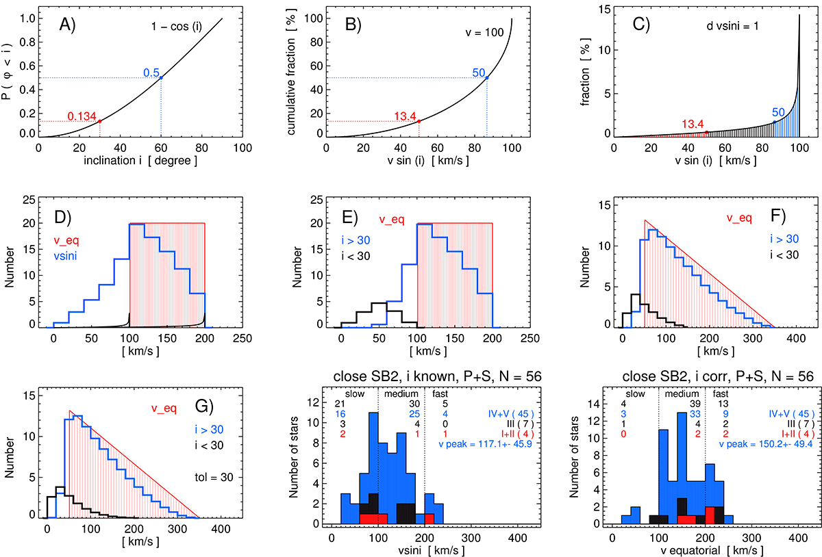
Fig. C.1.
Download original image
Effect of inclination. A: Fraction of axes at inclination ϕ < i vs i, assuming random inclinations. The red and blue dots mark two inclinations used in the discussion. B: Same as for A) but vs v sin i, adopting equatorial v = 100 km/s. C: Fraction of v sin i values for equidistant bins d v sin i = 1 km/s. The red and blue numbers give the cumulative contributions of the red and blue shaded area. D: Adopted constant distribution of stars with equatorial veq between 100 and 200 km/s (red shaded rectangle) and v sin i distribution resulting for random inclinations (blue histogram). The two black curves are the distribution in panel C scaled in v for 100 and 200 km/s. The blue histogram is constructed from the integration of all such black curves, it is scaled to the same area as the red histogram. About 30% of the stars from the rectangular red histogram will be observed with v sin i< 100 km/s. E: Same as for D) but separated with an inclination cut i > 30° (blue) and i < 30° (black). F: Same as for E) but adopting a triangular distribution of equatorial v between 50 and 350 km/s (red shaded). G: Same as for F) but allowing for a deviation between iorb and irot with a tolerance of 30° for co-axial rotation (Sect. C.3). The last two panels show the rotational velocity distribution of stars in close SB2 systems with known orbital inclination, without and with inclination correction (middle panel: v sin i, right: v equatorial).
Current usage metrics show cumulative count of Article Views (full-text article views including HTML views, PDF and ePub downloads, according to the available data) and Abstracts Views on Vision4Press platform.
Data correspond to usage on the plateform after 2015. The current usage metrics is available 48-96 hours after online publication and is updated daily on week days.
Initial download of the metrics may take a while.