| Issue |
A&A
Volume 692, December 2024
|
|
|---|---|---|
| Article Number | A132 | |
| Number of page(s) | 15 | |
| Section | Cosmology (including clusters of galaxies) | |
| DOI | https://doi.org/10.1051/0004-6361/202449952 | |
| Published online | 06 December 2024 | |
HOLISMOKES
XII. Time-delay measurements of strongly lensed Type Ia supernovae using a long short-term memory network
1
Max-Planck-Institut für Astrophysik,
Karl-Schwarzschild Str. 1,
85748
Garching,
Germany
2
Technical University of Munich, TUM School of Natural Sciences, Physics Department,
James-Franck-Str. 1,
85748
Garching,
Germany
3
Academia Sinica Institute of Astronomy and Astrophysics (ASIAA),
11F of ASMAB, No. 1, Section 4, Roosevelt Road,
Taipei
10617,
Taiwan
★ Corresponding author; This email address is being protected from spambots. You need JavaScript enabled to view it.
Received:
12
March
2024
Accepted:
8
July
2024
Abstract
Strongly lensed Type Ia supernovae (LSNe Ia) are a promising probe with which to measure the Hubble constant (H0) directly. To use LSNe Ia for cosmography, a time-delay measurement between multiple images, a lens-mass model, and a mass reconstruction along the line of sight are required. In this work, we present the machine-learning network LSTM-FCNN, which is a combination of a long short-term memory network (LSTM) and a fully connected neural network (FCNN). The LSTM-FCNN is designed to measure time delays on a sample of LSNe Ia spanning a broad range of properties, which we expect to find with the upcoming Rubin Observatory Legacy Survey of Space and Time (LSST) and for which follow-up observations are planned. With follow-up observations in the i band (cadence of one to three days with a single-epoch 5σ depth of 24.5 mag), we reach a bias-free delay measurement with a precision of around 0.7 days over a large sample of LSNe Ia. The LSTM-FCNN is far more general than previous machine-learning approaches such as the random forest (RF) one, whereby an RF has to be trained for each observational pattern separately, and yet the LSTM-FCNN outperforms the RF by a factor of roughly three. Therefore, the LSTM-FCNN is a very promising approach to achieve robust time delays in LSNe Ia, which is important for a precise and accurate constraint on H0.
Key words: gravitational lensing: strong / gravitational lensing: micro / supernovae: general / cosmological parameters / distance scale
© The Authors 2024
 Open Access article, published by EDP Sciences, under the terms of the Creative Commons Attribution License (https://creativecommons.org/licenses/by/4.0), which permits unrestricted use, distribution, and reproduction in any medium, provided the original work is properly cited.
This article is published in open access under the Subscribe to Open model.
Open Access funding provided by Max Planck Society.
1 Introduction
The Hubble constant, H0, is the present-day expansion rate of the Universe, which anchors the age and scale of our Universe. However, there is a significant discrepancy in H0 measurements coming from low redshifts, such as those using type Ia supernovae (SN Ia) in which the extragalactic distance ladder has been calibrated with Cepheids (e.g., Riess et al. 2018, 2019, 2021; Riess et al. 2022, 2024; Li et al. 2024; Anand et al. 2024), in comparison to high-redshift measurements extrapolated from the cosmic microwave background (CMB; Planck Collaboration VI 2020) by assuming the flat Lambda cold dark matter (ΛCDM) cosmological model. Independent investigations significantly lower the tension; for example, using the tip of the red giant branch to a sample of SNe Ia from the Carnegie-Chicago Hubble Program (Freedman et al. 2019, 2020; Freedman 2021). While Di Valentino et al. (2021) illustrate that low-redshift probes (e.g., Birrer et al. 2019; Kourkchi et al. 2020; Denzel et al. 2021; Riess et al. 2021) tend to have higher H0 compared to high- redshift ones (e.g., Planck Collaboration VI 2020; Balkenhol et al. 2021; Dutcher et al. 2021), it is unclear if the H0 tension can be resolved by unaccounted systematics in some of the measurements or if new physics beyond the successful ΛCDM model is required, such as curvature Ωk≠0, a dark-energy equation-of- state parameter, w≠−1 (i.e., non-constant dark energy density), a time-varying w, or a component of dark energy in the early Universe (e.g., Di Valentino et al. 2021; Schöneberg et al. 2022). To identify the origin of this problem, further independent and precise H0 measurements are required. Different groups tackle this task and methods like surface brightness fluctuations (e.g., Khetan et al. 2021; Blakeslee et al. 2021), the tailored- expanding-photosphere method of SN II (e.g., Dessart & Hillier 2005; Vogl et al. 2019, 2020; Csörnyei et al. 2023), megamasers (e.g., Pesce et al. 2020), and gravitational waves (e.g., Abbott et al. 2017; Gayathri et al. 2021; Mukherjee et al. 2021) have been used to successfully measure H0.
Another very promising approach to measure H0 in a single step, without calibrations of the extragalactic distance ladder, is lensing time-delay cosmography (Refsdal 1964) with strongly lensed supernovae (LSNe). Here, a supernova (SN) is lensed by an intervening galaxy or galaxy cluster into multiple images which appear at different moments in time, and therefore enable the measurement of a time delay between the LSN images. In addition to the time delay, a mass model of the lensing galaxy is required as well as a reconstruction of the mass along the line of sight. This method has been applied successfully to strongly lensed quasar systems (e.g., Bonvin et al. 2018; Birrer et al. 2019; Sluse et al. 2019; Rusu et al. 2020; Chen et al. 2019; Wong et al. 2020; Birrer et al. 2020), by the Time-Delay COSMOgraphy (TDCOSMO; Millon et al. 2020b) organization, consisting of members of the COSmological MOnitoring of GRAvItational Lenses (COSMOGRAIL; Courbin et al. 2018), the H0 Lenses in COSMOGRAIL’s Wellspring (H0LiCOW; Suyu et al. 2017), the Strong lensing at High Angular Resolution Program (SHARP; Chen et al. 2019), and the STRong-lensing Insights into the Dark Energy Survey (STRIDES; Treu et al. 2018) collaborations. Results from six strongly lensed quasars with well-motivated mass models (Wong et al. 2020), and also a seventh lens (Shajib et al. 2020), are in agreement with results from SNe Ia calibrated with Cepheids, but in 3.1σ tension with CMB measurements. A new analysis of seven lensed quasars (Birrer et al. 2020) lowers the tension, with the mass-sheet transformation (Falco et al. 1985; Schneider & Sluse 2014) only being constrained by stellar kinematics, leading to broadened uncertainties that are statistically consistent with the study from Wong et al. (2020) using physically motivated mass models. Even though LSNe are much rarer than lensed quasars, their advantages are their well-defined light curve shape and that they fade away with time, which enables follow-up observations of the lensing galaxy, especially to measure stellar kinematics (Barnabè et al. 2011; Yıldırım et al. 2017; Shajib et al. 2018; Yıldırım et al. 2020) for breaking model degeneracies, such as the mass-sheet degeneracy. Further, the fading nature of the SN helps one to derive a more precise lens model from the multiple images of the SN host galaxy, free of contamination from bright point sources (Ding et al. 2021). In this work, we focus on strongly lensed type Ia SNe (LSNe Ia), which are even more promising than other lensed SNe, given that SNe Ia are standardizable candles that allow one to determine lensing magnifications, and therefore yield an additional way to break degeneracies in the lens-mass model (Oguri & Kawano 2003; Rodney et al. 2015; Foxley-Marrable et al. 2018; Weisenbach et al. 2024; Pascale et al. 2024; Chen et al. 2024; Pierel et al. 2024a), provided that microlensing effects (whereby the stars of the lensing galaxy can significantly magnify and distort spectra and light curves of individual images (Yahalomi et al. 2017; Huber et al. 2019; Pierel & Rodney 2019; Huber et al. 2021; Weisenbach et al. 2021) can be mitigated.
To date, five LSNe Ia have been confirmed; namely, iPTF16geu (Goobar et al. 2017), SN 2022riv (Kelly et al. 2022), SN Zwicky (Goobar et al. 2022; Pierel et al. 2023), SN H0pe (Frye et al. 2024; Polletta et al. 2023; Pascale et al. 2024; Chen et al. 2024; Pierel et al. 2024a), and SN Encore (Pierel et al. 2024b), and in addition a Type Ia candidate called SN Requiem (Rodney et al. 2021). However, we expect to find between 500 and 900 LSNe Ia (Quimby et al. 2014; Goldstein & Nugent 2017; Goldstein et al. 2018; Wojtak et al. 2019; Arendse et al. 2024) with next-generation surveys, such as the upcoming Rubin Observatory Legacy Survey of Space and Time (LSST; Ivezic et al. 2019) over the duration of ten years. A more conservative estimate, considering only bright and spatially resolved LSNe Ia from Oguri & Marshall (2010, hereafter OM10) leads to 40 to 100 systems, of which, assuming sufficient follow-up observation (LSST-like 5σ depth, 2 day cadence), 10 to 25, depending on the LSST observing strategy, should provide accurate and precise time delays (Huber et al. 2019). Going one magnitude deeper in follow-up monitoring improves the number of LSNe Ia with well-measured time delays by roughly a factor of 1.5 (Huber et al. 2019). Using the current LSST baseline v3.0 cadence, Arendse et al. (2024) estimate ∼10 LSNe Ia per year that have time delays >10 days, >5 detections before light-curve peak, and are sufficiently bright (mi < 22.5 mag) for cosmological studies, corresponding to ∼100 LSNe Ia over the 10-year LSST survey. The LSST observing strategy is currently being optimized (Lochner et al. 2018; Lochner et al. 2022), which is important to maximize the number of LSNe Ia with a well-measured time delay. However, many different science cases depend on the LSST observing strategy, leaving only little room for optimization for the science case of LSNe Ia. Therefore, it is also very important to improve time-delay measurement methods, which is the scope of this work.
To measure the time delays between the multiple images of mock LSNe Ia, Huber et al. (2019) used the free-knot spline estimator from Python Curve Shifting (PyCS; Tewes et al. 2013; Bonvin et al. 2016). Another approach first suggested by Goldstein et al. (2018) uses color curves instead of light curves, in order to minimize the influence of microlensing (Goldstein et al. 2018; Huber et al. 2021). To calculate the microlensing effects on SNe Ia, theoretical models are required, where synthetic observables have been calculated with radiative transfer codes such as SEDONA (Kasen et al. 2006) or ARTIS (Kromer & Sim 2009). The theoretical models provide the specific intensity and therefore yield a spatial distribution of the radiation which can be combined with magnification factors coming from random source positions in a microlensing map (Vernardos & Fluke 2014; Vernardos et al. 2014, 2015; Chan et al. 2021) to calculate microlensed spectra, light curves, and color curves. Goldstein et al. (2018) found for the spherical symmetric W7 model (Nomoto et al. 1984) that the color curves are achromatic, meaning almost free of microlensing, up to three rest-frame weeks after explosion. We have confirmed this result for three other theoretical SN Ia models (Huber et al. 2021), testing also effects of asymmetries in the SN ejecta, although we have shown that, in practice, the usage of color curves is limited given that strong features such as peaks are only present in three out of five independent LSST color curves (coming from ugrizy), which would require follow-up observations in rizyJH for typical source redshifts of LSNe Ia, where it will be especially challenging to get good quality data in the redder bands. However, this will improve significantly with the upcoming Roman Space Telescope that will observe in the infrared (Spergel et al. 2015; Rose et al. 2021; Pierel et al. 2021).
Still, Huber et al. (2022) investigated the usage of light curves further to measure time delays between the resolved images of LSNe Ia using two simple machine-learning techniques: (i) a deep learning fully connected neural network (FCNN) with two hidden layers, and (ii) a random forest (RF; Breiman 2001) that is a set of random regression trees. The data for a FCNN or a RF require always the same input structure and size and since LSNe Ia have a variable amount of observed data points, a machine-learning network needs to be trained for each observed LSN Ia individually. To include microlensing in the simulations, Huber et al. (2022) trained on four theoretical SN Ia models also used in Suyu et al. (2020) and Huber et al. (2021). While the results on a test set based on the same four theoretical models look very promising for the FCNN and the RF, tests of generalizability, using empirical light curves from the SNEMO15 model (Saunders et al. 2018) show that only the RF provides almost bias-free results. For the RF we can achieve an accuracy in the i band within 1% for a LSN Ia detected about eight to ten days before peak, if delays are longer than 15 days. The precision for a well sampled LSNe Ia at the median source redshift of 0.77 is around 1.4 days, assuming observations are taken in the i band for a single-epoch 5σ depth of 24.5 mag with a cadence of 2 days. Another important point is that for typical LSNe Ia source redshifts between 0.55 and 0.99 (16th to 84th percentile of LSNe Ia from OM10), the i band provides the best precision, followed by r and z (or g if zs ≲ 0.6), where the best performance is achieved if a RF is trained for each filter separately. Further results are that the observational noise is by far the dominant source of uncertainty, although microlensing is not negligible (factor of two in comparison to no microlensing) and that there is no gain in training a single RF for a quad LSNe Ia instead of a separate RF per pair of images, that means treating it like a double system. Furthermore, from the RF we can expect slightly more precise time-delay measurements than with PyCS used by Huber et al. (2019).
Another time-delay measurement tool was developed by Pierel & Rodney (2019), which uses SN templates from empirical models, but microlensing on LSNe Ia is approximated as wavelength independent1, in contrast to Huber et al. (2022), where microlensing is calculated from the specific intensity profiles of theoretical models. Further, Bag et al. (2021), Denissenya & Linder (2022), and Bag et al. (2024) show that time-delay measurement of unresolved LSNe in LSST might be possible using machine learning if they are classified correctly as LSNe.
The main disadvantage of the machine-learning models trained by Huber et al. (2022) is that the same input structure and amount of data points are required, meaning that a model needs to be trained for each observation of a LSN Ia individually. Therefore the goal of this work is to develop a much more general method that can handle LSNe Ia of almost any kind and ideally also outperforms the RF. Specifically, we use a Long Short-Term Memory Network (LSTM), which is well suited to handle time-dependent problems (Hochreiter & Schmidhuber 1997), in combination with a FCNN, which we refer to as LSTM- FCNN. In this work, we investigate only LSNe Ia, although the techniques can be also applied to other types of SNe. Applications to other SN types require, however, mock microlensed light curves of these SNe, which are beyond the scope of this paper to produce. The number of LSNe II is slightly higher than the number of LSNe Ia, which makes them also promising for timedelay cosmography. A study on LSNe IIP using spectra and color curves for the time-delay measurement was done by Bayer et al. (2021).
This paper is organized as follows. In Sect. 2 we explain the production of our dataset for our machine-learning model, which will be explained in Sect. 3, before we present our results in Sect. 4. In Sect. 5 we apply the LSTM-FCNN to specific configurations and compare results to previous ones presented in Huber et al. (2022). Finally, we summarize in Sect. 6. Magnitudes in this paper are in the AB system. To calculate distances we assume a flat ΛCDM cosmology with H0 = 72 km s−1 Mpc−1, Ωr = 0 (for radiation) and Ωm = 0.26 (for matter).
2 Dataset for machine learning
In this section, we explain the production of the dataset to train, validate, and test our LSTM model. The calculation of microlensed light curves with observational noise is described in Sect. 2.1 and the creation of the dataset used in this work is explained in Sect. 2.2.
2.1 Microlensed light curves with observational noise
The calculation of microlensed light curves is described in detail in Huber et al. (2019) and the calculation including the observational noise, especially for different moon phases can be found in Huber et al. (2022). In the following we summarize the most important points.
To calculate light curves including microlensing, a theoretical SN model is required. We use four of these models to increase the variety: (1) the W7 model (Nomoto et al. 1984), that is a parametrized 1D deflagration model of a Chandrasekhar- mass (Ch) carbon-oxygen (CO) white dwarf (WD), (2) the delayed detonation N100 model (Seitenzahl et al. 2013) of a Ch CO WD, (3) a sub-Chandrasekhar (sub-Ch) detonation model of a CO WD with 1.06 solar masses (Sim et al. 2010), and (4) a merger model of two CO WDs with solar masses of 0.9 and 1.1 (Pakmor et al. 2012). The theoretical models are used in combination with magnification maps from GERLUMPH (Vernardos & Fluke 2014; Vernardos et al. 2014, 2015) to calculate the microlensed observed flux via:
 (1)
(1)
with the luminosity distance to the source Dlum, the source redshift zs, the magnification factor µ(x, y), and the emitted specific intensity at the source plane Iλ,e (t, p), which is a function of wavelength, λ, the time since explosion, t, and the impact parameter, p, that is, the projected distance from the ejecta center, where spherical symmetry is assumed following Huber et al. (2019, 2021). The magnification maps which provide the magnification factor µ(x, y) as a function of the source positions (x, y) depend on three main parameters, the convergence κ, the shear γ, and the smooth matter fraction s = 1 − κ*/κ, where κ* is defined as the convergence of the stellar component. Further, these maps also depend on the source redshift zs and lens redshift zd, that set the Einstein radius REin and thus the characteristic size of the map. The microlensing magnification maps are created following Chan et al. (2021), where the maps in Huber et al. (2022) and in this work use a Salpeter initial mass function (IMF) with a mean mass of the microlenses of 0.35 M⊙ and a resolution of 20 000 × 20 000 pixels with a total size of 20 REin × 20 REin.
From the observed microlensed flux from Eq. (1) we obtain the microlensed light curves in AB magnitudes via
 (2)
(2)
(Bessell & Murphy 2012). Further, c is the speed of light and the transmission function for the filter X is SX(λ). From Eq. (2) we can then calculate magnitudes with observational uncertainties via
 (3)
(3)
where rnorm is a random number following a Gaussian distribution with zero mean and a standard deviation of one. The 1σ standard deviation of mX(t) is σX(t), which depends mainly on mAB,X(t) relative to the 5σ depth of the filter X (see LSST Science Collaboration (2009), Sect. 3.5, p.67, Huber et al. (2022), and Appendix A). In this work we assume as in Huber et al. (2022) that follow-up observations will be triggered for the LSNe Ia detected by LSST to get better quality light curves with a mean single-epoch LSST-like 5σ depth plus one; that is, 24.5 mag for the i band, which is feasible even with a 2-meter telescope (Huber et al. 2019). Further, we assume as in Huber et al. (2022) a time-varying 5σ depth to account for the moon phase.
2.2 Dataset for a long short-term memory network
In this section we describe the production of the dataset for the LSTM network, which is more general than the RF from Huber et al. (2022) since LSTM’s architecture can handle most LSNe Ia expected from OM10, without the requirement of specific training for a particular observational pattern. Our training set is composed of a sample of 200 000 LSNe Ia and the validation and test set each have a size of 20 000. A single sample S contains all observed data points for each of the two images of a LSNe Ia, where a single data point k of image j is represented by
 (4)
(4)
where tjk is the time when the magnitude mjk of image j is observed with the 1σ uncertainty of σjk. Since we investigated only the i band in this work, we drop the filter notation as introduced in Eq. (3). Therefore, the single sample S , containing a single LSN Ia, can be written as
 (5)
(5)
where Nsl,1 and Nsl,2 are the number of observed data points as in Eq. (4) for image one and two, which we also refer to as sequence length. The  , respectively
  , contains the sequence of observed data points for image one, respectively, image two. If we consider multiple samples, we labeled them by l leading to
  with Nsl,1,l and Nsl,2,l for the sequence length of image one and two of the l-th sample.
A random set of LSNe Ia systems used for our training process is shown in Fig. 1, where the left four panels show the data without normalization. The right four panels show the same four samples with normalization, which will be used in our machinelearning network, where we use all data points (as in Eq. (4)) from the two images as input to predict the time delay Δt between these images. The applied normalization is very important such that the input values for the LSTM network have always the same order of magnitude. Therefore, we normalized the magnitude of both images with respect to the peak of the image under consideration. Given that very noisy data points can be brighter than the peak we only considered 25% of the data points with the lowest uncertainty to find the peak (minimum in magnitude). We then subtracted the peak magnitude from each data point in the corresponding light curve, such that the peak has a magnitude value of zero. Furthermore, we also normalized the time scale t, which in our case is the time after explosion, by adding a constant offset to t such that the offset t = 0 corresponds to the peak determined for the first image. We then divided the time delay, Δt, and time scale, t, by 150 days, which is the maximum of the time delays under consideration, such that the output of the LSTM network is restricted to values between 0 and 1. Given that we are primarily interested in measuring the time delay(s) from the light curves, our introduced normalization disregards the relative magnifications between the two images. While relative and absolute magnifications are useful properties, determining them is nontrivial, especially since they can vary over time due to the effects of microlensing. Obtaining relative or absolute magnifications in conjunction with redshift would necessitate a new neural network or method, which is beyond the scope of this work but could be of interest for future projects.
In the following, we explain how such a random dataset is created, where we summarize the variety of lensed SNe that we consider in Table 1. To simulate light curves for LSNe Ia, we used the four theoretical models described in Sect. 2.1 and the empirical SNEMO15 model (Saunders et al. 2018), which contains 171 SN Ia light curves. To ensure that we have light curves not used in the training process to test the generalizability, we randomly splitted the whole SNEMO15 dataset into three subsets: (1) SNEMO15-T consisting of 87 curves for training, (2) SNEMO15-V consisting of 42 curves for validation, and (3) SNEMO15-E consisting of 42 curves for testing. Our training, validation, and test set is then composed of 50% light curves from theoretical SN models and 50% of empirical light curves from the corresponding subset of SNEMO15 light curves. Furthermore, we constructed a second test set to investigate the generalizability, namely the SNEMO15-only test set, based only on the 42 light curves in SNEMO15-E. A summary of all datasets is listed in Table 2.
For each theoretical model, we undertook calculations for a given LSN Ia image, 10 000 microlensed light curves from the corresponding microlensing map of the LSN Ia image (set by κ,γ, s, zs, zd), as was described in Sect. 2.1. Since the calculation of microlensed SN Ia light curves is very time consuming, we only investigated a subset of microlensing magnification maps, while covering a broad range of properties of the LSN Ia image. The upper panel of Fig. 2 shows the distribution of (κ, γ) values from the OM10 catalog and the six pairs used in this work, which are composed of the median and two systems on the 1σ contours, taken separately for the lensing image types “minimum” and “saddle”. Furthermore, we assumed three typical s values of 0.4, 0.6, and 0.8 similar to Huber et al. (2019, 2021, 2022) and five different pairs of (zs , zd), as shown in the lower panel of Fig. 2 also based on the OM10 catalog. Therefore we investigated in total 6 × 3 × 5 = 90 different microlensing magnification maps where we calculate for each map 10 000 random source positions for all four theoretical models providing 90 × 10 000 × 4 = 3 600 000 microlensed SN Ia light curves, which is more than sufficient given that Huber et al. (2022) found that microlensing is not the dominant source of uncertainty.
For the empirical SNEMO15 model, no specific intensity profiles are available, and therefore the calculation of microlensed light curves described in Sect. 2.1 is not possible. To nonetheless include microlensing effects, we use the theoretical models where we subtract from a randomly selected microlensed light curve (which include macrolensing plus microlensing) the macrolensed light curve, assuming µmacro = 1/((1 − κ)2 − γ2), to get only the contribution from microlensing which we then add to a SNEMO15 light curve. With the six pairs of κ and γ, we only covered a small part of potential macrolensing factors; however, from Fig. 3, we see that the microlensed light curves from these six pairs span a much broader range of potential magnification factors as we would get from macrolensing only, from the whole OM10 sample.
The source redshift and the lens redshift together set the scale of the microlensing map, and affect only weakly the microlensing effect on SN Ia light curves (Huber et al. 2021). However, the source redshift also determines the observed light curve shapes and brightness in a certain band. Since Huber et al. (2022) showed that in terms of noise contributions, the observational noise is far more important than microlensing, and the five source redshifts shown in Fig. 2 are sufficient for the microlensing calculation, but not for the various brightness and light curve shapes coming from the OM10 sample, which include zs between 0.17 and 1.34. Therefore, we drew randomly pairs of (zs,OM10, zd,OM10) from the OM10 catalog and we picked from the lower panel of Fig. 2 the pair (zs,micro, zd,micro) from our used sample (in red) which is closest. We have then rescaled the pre-calculated microlensed flux  for the source redshift zs,micro to zs,OM10, the random source redshift of interest:
 (6)
(6)
Further, we rescale as well the wavelength
 (7)
(7)
and time since explosion
 (8)
(8)
With Eq. (2) we can then calculate the microlensed light curves for zs,OM10, providing the correct light curve shape and brightness but only approximated microlensing contributions.
For our dataset, we further considered a range of the followup strategy, namely we pick for each simulated sample randomly a cadence of 1, 2, or 3 days with a random uniform scatter of ±4 hours, given that we will not always observe at the exact same time in a night. Further, we assumed a depth 1 mag deeper than the mean LSST single-epoch 5σ depth, which provides a good compromise between required time on a hypothetical 2m telescope on the one hand and accurate or precise time delays in LSN Ia systems on the other hand (Huber et al. 2019). In reality we will not be able to observe with a regular cadence because of, for example bad weather, and therefore we randomly deleted between 0 and 50% of the times follow-up observations are assumed. Furthermore, we limited the discoveries of the first image of a LSN Ia to a detection not later than 5 days after peak, which is the aim of our lens finding approaches. For simplicity, we only train the network in the i band, given that this provides by far the most precise time-delay measurement (Huber et al. 2022). From Eq. (3) we see that extremely high uncertainty values are possible, which occur only rarely in practice and can be easily removed from the data. Therefore, we will only take data into account where the standard deviation σik of an observed data point mik is smaller than 2 mag.
The theoretical light curves used in the training process match only partly the empirical SNEMO15 light curves as can be seen from Fig. 4 for typical source redshifts. To increase the variety of the light curve shapes from theoretical models we multiplied a random factor between 0.7 and 1.3 to the time after explosion to stretch and squeeze the light curves and add a random shift in magnitude between −0.4 and 0.4 to vary the brightness, given that Huber et al. (2022) have shown that this helps the FCNN and the RF best to generalize better to SN models not used in the training process. This leads to absolute magnitudes from −17.9 to −19.7 in u band and −18.7 to −19.7 in ɡ band. Further, our underlying light curves from theoretical and empirical models covered a range from ∼3.4 to 70.0 rest-frame days after explosion.
Finally, to create a training, validation, or test set, we randomly picked a time delay between 0 to 150 days for each LSN Ia system, and decided if our LSN Ia light curves will be based on a theoretical model or the empirical model (including microlensing from a theoretical model) with equal probability. For the theoretical model, we decided with a 50:50 chance if we use the theoretical models shown in Fig. 4 or if we apply a random stretching factor between 0.7 and 1.3 and a random shift in magnitude between −0.4 and 0.4. Further, we pick randomly for the first image a minimum ((κ, γ) = (0.37, 0.35), (0.27, 0.24), or (0.46, 0.48)) and for the second image a saddle ((κ, γ) = (0.69, 0.7), (0.9, 0.9), or (0.52, 0.53)), as well as a source redshift from the OM10 sample, for which we approximate the microlensing contribution following the process described in Eqs. (6)–(8). Given that the empirical SNEMO15 model covers rest-frame wavelengths only between 3305 and 8586 Å, we cannot calculate i-band light curves for zs > 1.0; therefore, if the empirical model is picked for such a high zs , we drew the redshift again until we have zs ≤ 1.0. Furthermore, we drew a random position in the moon phase and assume the detection and follow-up strategy described previously. For this specific random setup, we created then four samples described by Eq. (5) for the four theoretical SN Ia models, or if the empirical model is picked we use, for example for the training set, one of the 87 SNEMO15-T light curves, where we created also four samples with four different microlensing contributions from the four theoretical models. For this specific setup we calculated then the microlensed SN Ia light curves with random noise following Eq. (3), leading to samples shown on the left hand side of Fig. 1. We repeated the previously described procedure by drawing new time delays until we reached the target size of a certain dataset. For the training set, we used 200 000 samples, and the validation and test sets contained each 20 000 samples.
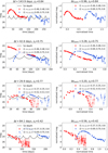 |
Fig. 1 Four random samples of our training set, comparing data without normalization (left panels) and data with normalization (right panels) that will be used for our machine-learning network. The red and blue data points are the i-band light curves for the first and the second, respectively, lensed SN image. The black curves in the left panels show the i-band 5σ limiting depth, which oscillates with the moon phase. The normalization procedure to obtain the right panels from the left panels is described in Sect. 2.2. |
Summary of our inputs for the LSTM dataset used for training, validation, and testing.
Description of the training, validation, test, and SNEMO15-only test set used in this work.
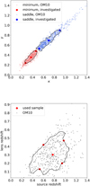 |
Fig. 2 Convergence κ and shear γ (upper panel), and source redshift zs and lens redshift zd (lower panel) used for the calculation of microlensed light curves drawn from the OM10 catalog. The black lines represent contours that enclose 68% of the LSN Ia systems in the OM10 catalog. |
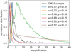 |
Fig. 3 Distribution of magnification factors from the six microlensed magnification maps under investigation in this work (solid colored), in comparison to all macro-magnification factors from all LSNe Ia from the OM10 catalog (dashed black). Microlensing magnification maps investigated in this work cover a much broader range of potential magnification factors in comparison to the macrolensing only case from the whole OM10 sample. |
3 Machine-learning technique
In Sect. 3.1 we summarize briefly the basic concept of an LSTM network before we introduce our setup in Sect. 3.2.
3.1 Basics of Long Short-Term Memory Network
The LSTM network (Hochreiter & Schmidhuber 1997; Sak et al. 2014; Sherstinsky 2020) is motivated by the Recurrent Neural Network (RNN), where both have the purpose to solve a timedependent problem. For the RNN, the basic setup is illustrated in Fig. 5 for the k-th time step. We have an input vector xk for which we calculate the state Ak by using information of the previous time step k − 1 to further calculate the output hk . In equations, ignoring non-linear activation functions, this can be expressed as
 (9)
(9)
and
 (10)
(10)
where wA , wx, and wh are the time-step independent weights that are learned in the training process via backpropagation. The main issue with RNN is that they have the tendency of exploding or vanishing gradients, which makes it very difficult to learn long-term dependencies (Pascanu et al. 2013; Philipp et al. 2018).
To overcome that issue, LSTM network have been introduced by Hochreiter & Schmidhuber (1997), where we have in addition to the hidden state hk , a cell state ck , that acts as a memory. Furthermore, the state Ak is replaced by a more complex unit, as is shown in Fig. 6, which contains the following main ingredients with ⊙ denoting the Hadamard product3:
 (11)
(11)
 (12)
(12)
 (13)
(13)
 (14)
(14)
 (15)
(15)
 (16)
(16)
where the sigmoid and tanh activation functions act on each element of the vector. The input vector at time step k is xk with size Ninput, which is, in our case, three, containing the time, magnitude, and uncertainty as listed in Eq. (4). The hidden state hk is a vector with size Nhidden. The biases bi, bf , bg, and bo are vectors with size Nhidden, the weights wXf, wxg, wxi, and wxo are Nhidden × Ninput matrices, and the weights whf , whg, whi, and who are Nhidden × Nhidden matrices. The biases and weights are not dependent on the time step and are learned through backpropagation in the training process. The hidden state hk is the prediction of the LSTM network at time step k and serves as input to calculate the hidden state hk+1 corresponding to the time step k + 1. The cell state ck acts as memory and transports information through the unit. The forget gate fk decides on when and which parts to erase from the cell state. The gate gk removes or adds information to the cell state coming from the input gate ik . The output gate ok is responsible for the output and hidden state hk of the LSTM network. Outputs are produced at every time step, but for our case, we will only use the last output at time-step Nsl , after the full light curve with the sequence length of Nsl was propagated through the network. This corresponds to a many-to-one scenario where we have Nsl input data points as in Eq. (4) for which we predict one time delay Δt and the uncertainty of the time delay σΔt.
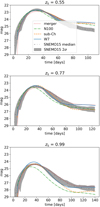 |
Fig. 4 i band light curves for typical source redshifts of LSNe Ia as indicated on the top of each panel. We compare four theoretical models (merger, N100, sub-Ch, and W7) with the empirical SNEMO15 model. |
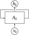 |
Fig. 5 Illustration of an RNN. The input xk is used to calculate state Ak of the network at the k-th time step, by using also the information from the previous k − 1 time step. The output hk is then computed from the state Ak. See Eqs. (9) and (10). |
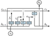 |
Fig. 6 Illustration of an LSTM. The input xk is used in combinations with the output hk−1 and the cell state ck−1 from the previous time step k − 1 to produce the output hk for the k-th time step. The cell state ck acts as memory and transports information through the cell, where the forget gate fk , input gate ik , and gate gk update information in the cell state. The output gate, based on the previous output hk−1 and input xk in combination with information from the cell state provides the new output hk. For more information, see Eqs. (11)–(16). |
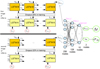 |
Fig. 7 Illustration of our LSTM-FCNN composed of a Siamese LSTM network and a FCNN with two hidden layers. Details about the LSTM cells are shown in Fig. 6. Both sub-LSTM networks for image one (top, input denoted by S 1k) and image two (bottom, input denoted by S2k) are the same LSTM network (i.e., with the same weights in the neural network) composed of 2 layers (LSTM A and LSTM B) where during the training process, a dropout rate of 20% is used. We use only the last outputs |

3.2 Modified Siamese long short-term memory network
For our approach, we used a Siamese LSTM network (Bromley et al. 1993). The Siamese neural networks are in general a class of neural network architectures that contain two or more identical sub-networks, which therefore have the same weights and parameters. A Siamese LSTM is also used in the Manhattan LSTM (MaLSTM) network (Mueller & Thyagarajan 2016) developed to find semantic similarities between sentences. In this network two sentences with different (or the same) number of words are feed through the same LSTM network to predict an output for each sentence. The two outputs are then used to calculate a Manhattan distance which states the similarity between the two input sentences.
Our approach is similar to the MaLSTM, but instead of sentences, we have different images of a LSN Ia, and instead of a single word, we have the time of the observation, the magnitude, and the uncertainty of the measurement shown in Eq. (4). Our approach produced similar to the MaLSTM two outputs for the two images, but instead of using a Manhattan distance, we used a FCNN with two hidden layers, given that we wanted to determine a time delay instead of a similarity score.
Our full LSTM-FCNN is shown in Fig. 7, where the calculations of the LSTM network are listed in detail in Eq. (11)–(16), where we added a second index, j, to the time step, k, leading to hjk, Cjk, fjk, gjk, ijk, and ojk in order to distinguish between image one (j = 1) and image two (j = 2) of our lensed SN system. Our network takes as input the data S1k of image one and S2k of image two, and predicts as an output, the time delay Δt and the uncertainty of the time delay σΔt. The sub-LSTM networks for both images are identical and composed of the two layers LSTM A and LSTM B. The second layer of the LSTM network takes as input, the output from the first layer  , where a dropout rate pdropout = 20% is applied, meaning that during the training process randomly 20% of the input data for the second layer
  are set to zero and the other values are rescaled by 1/(1-pdropout). The rescaling is necessary given that the dropout is just applied in the training process but not during the validation and test phase, which would lead to systematically larger outputs for the validation and test set if the re-scaling in the training process would not be applied. The dropout helps the network to avoid focusing on very specific nodes during training in order to generalize better to data not used in the training process. The last two outputs from the second layer,
  for image one and
  for image two, are then concatenated and used as input for the FCNN.
For given j and k, the inputs Sjk are vectors with size of 3 (see Eq. (4)) whereas the outputs from both layers  and hjk are vectors with size Nhidden = 128. Therefore, the input layer of the FCNN has 256 nodes, which we summarize in a vector d:
 (17)
(17)
with dimension 256. The two hidden layers of the FCNN have 128 and 10 nodes, where at each hidden layer, a non-linearity is applied by using a rectified linear units (ReLU) activation function (e.g., Schmidt et al. 1998; Maas et al. 2013), which is the identity function for positive values and zero for all negative values. In the last layer where final outputs are produced, a sigmoid activation is used which predicts values between 0 and 1 and therefore covers the range of potential normalized time delays.
The first hidden layer is represented by the vector η1 with size 128 and the second hidden layer by the vector η2 with size 10:
 (18)
(18)
 (19)
(19)
The outputs of the network are then two scalar values, namely the normalized time delay Δtnorm and the normalized variance “Var”:
 (20)
(20)
where, ω1 (matrix of size 128 × 256), ω2 (matrix of size 10 × 128), and ω3 (matrix of size 2 × 10) are the weights, and β1 (vector of size 128), β2 (vector of size 10), and β3 (vector of size 2) are the biases. Weights and biases of the network are learned in the training process. Further, the outputs from Eq. (20) need to be translated to a physically meaningful Δt and  . For the time delay, this is straight forward by just removing our normalization factor:
 (21)
(21)
but for  this is not as trivial and we will explain our approach in Sect. 4.
For the implementation of the LSTM-FCNN, we used the machine-learning library PyTorch (Paszke et al. 2019), where we train for a certain number of epochs until a generalization gap becomes visible (more details in Sect. 4). In each epoch, we subdivide our training set randomly into mini batches with size Nbatch = 128. Given that image one and image two of the 128 samples (labeled as l) of a mini batch have a different sequence length Nsl,1,l and Nsl,2,l, we pad them with zeros at the end until all mini-batch samples of image one have a shape of (max(Nsl,1,l), 3) and all samples of image two have a shape of (max(Nsl,2,l), 3), where the 3 is coming from the three inputs from Eq. (4). The padding is required such that the PyTorch class torch.nn.LSTM can handle variable sequence lengths within a mini batch4. As input for the FCNN, we use for each sample l the last unpadded output at time step Nsl,1,l for image one and Nsl,2,l for image two, which are then combined to predict Δt and σΔt . For each sample of the mini batch, we can then compute the performance of the LSTM-FCNN by using the Gaussian negative log likelihood (Nix & Weigend 1994) as the loss function:
 (22)
(22)
where є = 10−6, is used for stability. The true normalized time delay of the training sample is Δtnoɪm,true and Δtnorm is the time delay predicted from the network. Furthermore, we used the second “raw” output of the LSTM-FCNN as the variance “Var” as in Eq. (20). The advantage of the Gaussian negative log likelihood loss in comparison to the mean squared error loss used in Huber et al. (2022) is that we not only optimize such that the predicted time delay of the network is close to the true time delay, but we also get an approximation of the uncertainty for each sample. The loss is then used for the backpropagation to update the weights and biases of the LSTM-FCNN. For this we use the Adaptive Moment Estimation (Adam) optimizer (Kingma & Ba 2014) with a learning rate α = 0.000005.
The network with our specific choices and values of Nhidden , Nbatch , α, number of LSTM layers, dropout rate, FCNN with two hidden layers and so on is of course somewhat arbitrary, although the setup of the FCNN was motivated by Huber et al. (2022). However, we also investigated other setups for a smaller training sample, for example, Nhidden = 64, 256, or 512, Nbatch = 64, 256, or 512, just one LSTM layer without dropout and so on, and we found that the performance of these networks were typically very similar or ~ 10 percent worse than our chosen setup. Therefore, given that the training of a single setup of such an LSTM network takes several weeks on a GPU node (NVIDIA A10) and that we found only minor performance differences for a few tested configurations of the LSTM-FCNN, we skipped a huge grid search for all potential hyperparameters, which is also justified by the performance of our LSTM-FCNN already achieving our target precision and accuracy.
4 Results
In Sect. 4.1 we describe how the LSTM-FCNN is trained, in Sect. 4.2 we evaluate the performance by applying it to our test sets and in Sect. 4.3 we describe the uncertainty prediction of the network.
4.1 Training process
To evaluate the performance of our LSTM-FCNN on a given dataset (e.g., training set, validation set, test set), we calculate for each sample as in Eq. (5), now labeled as l, the time-delay deviation via,
 (23)
(23)
comparing the true time delay Δttrue,l to the predicted one from the network Δtpгed,l. Given that our data is normalized in time for the input and output of our LSTM-FCNN, we need to undo the normalization as in Eq. (21) to get the time delays in days. We can then estimate the bias (also referred to as accuracy) by using the median  and the precision by using the 84th percentile τ p,84 and the 16th percentile τp,16 from the whole sample (200 000 for the training data and 20 000 for each of the other datasets). The results are then summarized in the following form:
 (24)
(24)
We trained our LSTM-FCNN described in Sect. 3.2 with the dataset as described in Sect. 2.2, using light curves from theoretical and the empirical SNEMO15 models listed in Table 2.
Our training process lasted for ~40 000 epochs and we used the LSTM-FCNN at the epoch where the validation set has the minimum loss value calculated from Eq. (22) with the additional requirement that the bias as defined in Eq. (24) at this epoch is lower than 0.05 day, to ensure that at least for the validation set, a time delay longer than 5 days would be enough to achieve a bias lower than 1%. The loss curve for the training and validation set as a function of the training epoch is shown in Fig. 8, where we see the generalization gap beyond epoch ∼15 000, and we reached the lowest validation loss with low bias at epoch 21817, which is the status of the LSTM-FCNN as used further in this work. Even though the training of the network took several weeks on an NVIDIA A10 GPU node, after successful training, applying the LSTM-FCNN to a single LSNe Ia takes only a negligible amount of time (less than one second). The fast evaluation arises from the straightforward calculations outlined in Sect. 3.2 and illustrated in Fig. 7, where a time delay with its corresponding uncertainty estimate is directly derived from the data points of the two images of an LSNe Ia without fitting specific models to them.
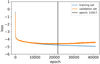 |
Fig. 8 Training and validation loss of the LSTM-FCNN as a function of the training epoch. The vertical line marks the state at which we use the LSTM-FCNN where the validation loss is the lowest with the additional requirement that the bias is lower than 0.05 day. The plot shows that with more training epochs the network improves its performance while around epoch 22 000 the validation loss starts to increase again while the training loss still decreases because the LSTM-FCNN starts to overfit, meaning that, for example, it fits to specific noise patterns present in the training set. |
4.2 Performance
For our LSTM-FCNN we calculate the time-delay deviation for the training set, validation set, test set, and SNEMO15-only test set which is shown in Fig. 9. We see that our network performs very well with almost zero bias and a precision on the order of 0.7 days, which can be also achieved on light curve shapes never used in the training process, as represented by the SNEMO15-only test set.
Further, we tested how the performance changes if we create five SNEMO15-only test sets with a fixed cadence of 1, 2, 3, 4, and 6 days. We find that as long as the cadence is part of our training data (1, 2, or 3 days), the bias is negligible, but the precision degrades from ∼0.6 days for a daily cadence to ∼1.1 days for a cadence of 3 days. For a cadence of 4 or 6 days, which is not part of the training data, we see that a bias emerges. Details can be found in Appendix B. If the LSTM-FCNN should be applied to a more sparsely sampled light curve than assumed in our training data, the training of a new LSTM-FCNN is required. Current dedicated monitorings of lensed quasars (e.g., Millon et al. 2020a) have demonstrated that a cadence of ∼1-2 days are achievable, especially when missing data due to, for example, weather and telescope maintenance, are accounted for (which we have incorporated in our simulated light curves by dropping up to 50% of the data points, randomly chosen for each sample). Therefore, with such dedicated monitoring in the i-band, our existing LSTM-FCNN network is readily applicable.
As an additional test, we applied the LSTM-FCNN to a completely independent dataset based only on the SALT3 (Kenworthy et al. 2021) SN Ia model. Furthermore, we drew time delays, κ, and γ randomly from OM10, where we considered only the effect of macrolensing. Even though we applied major changes to our assumptions made in Table 1 in generating this SALT3 test set, our network still performed very well. The small bias of −0.16 days is negligible if we restrict ourselves to time delays longer than 16 days in order to achieve an accuracy better than 1%. In the future, when even more general LSTM-FCNN will be trained, it might be interesting to add as many models as possible to the training dataset to reduce the bias on unseen data even further.
Our LSTM-FCNN is constructed such that the image which arrives first needs to be the first input and the second arriving image is required as the second input. For short time delays (Δt ≲ 10 days) it might not always be possible to distinguish between the first and second image. However, in practice this is not a problem as the LSTM-FCNN ouputs typically a value very close to zero if the input of the two images has the wrong order. Therefore, when we test our network, we try as input both potential orders of the two images and always take the higher time delay as the predicted one. This is already done for the test set and SNEMO15-only test set in Fig. 9. The presented result would be exactly the same if we input the images always in the right order, and therefore, we see that this limitation of our LSTM-FCNN is not a problem in practice.
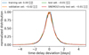 |
Fig. 9 Evaluation of the LSTM-FCNN on the training set, validation set, test set, and SNEMO15-only test set. With a 1σ spread of ∼0.7 days and almost no bias even on the two test sets, the LSTM-FCNN is very promising for future measurements of time delays from real LSNe Ia. |
4.3 Uncertainty estimate
In order to relate the raw Var output from our LSTM-FCNN also listed in Eq. (22) to a meaningful σΔt, we used the validation set shown in Fig. 9. To convert the Var output, we first calculated the rescaled uncertainty prediction from the network
 (25)
(25)
where the factor 150 comes from the normalization of our timescale described in Sect. 2.2. In a next step, we applied the LSTM-FCNN to the full validation set and plot for each sample the time-delay deviation (as defined in Eq. (23)) over the rescaled predicted uncertainty of the network, σpred , as is shown in Fig. 10, where we fit a normal function to it. Although the normal function fits the distribution overall well, the outer regions, where the predicted time delay Δtpred is more than 2σpred away from the true time delay Δttrue, are not represented very well. Therefore, we looked at different confidence intervals of the validation set, which yielded a correction factor, as is shown in Figure 11. The final uncertainty estimate for the 64th, 95th, and 99.7th confidence interval of a single sample can then be calculated via
 (26)
(26)
 (27)
(27)
and
 (28)
(28)
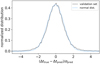 |
Fig. 10 Application of the LSTM-FCNN to the validation set. The distribution shows the time-delay deviation of each sample over the predicted uncertainty of the network. In blue we see a fit with a normal distribution. |
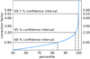 |
Fig. 11 Based on Fig. 10 we can define confidence intervals and find based on the fit function f a correction factor that needs to be applied to the predicted uncertainty of the network σpred. |
5 Specific applications of the LSTM-FCNN and comparison to other methods
In this Section, we applied the LSTM-FCNN to more specific examples to compare the performance to the results from Huber et al. (2022). In particular, we created a dataset, as described in Sect. 2, but we fixed zs , κ, γ, and s to very specific values as used by Huber et al. (2022), where a system was picked from the OM10 catalog with a source redshift zs = 0.76 that is closest to the median source redshift zs = 0.77 of the OM10 catalog. The specific system is a double LSN Ia with (κ1, γ1, s1) = (0.25, 0.27, 0.6) for the first SN image and (κ2,γ2, s2) = (0.83, 0.81, 0.6) for the second SN image. For this system Huber et al. (2022) investigated different scenarios of at peak and before peak detection. Fig. 12 shows our LSTM-FCNN on a SNEMO15-only test set, based on (κ1,γ1, s1) = (0.25, 0.27, 0.6) and (κ2, γ2, s2) = (0.83, 0.81, 0.6) for four different times of detection.
We first see that even though the specific κ and γ values are not part of our training data (Table 1), the network predicts very accurate and precise time delays. Further, we see that the precision drops with fewer data points before peak, although at-peak detection still yields an uncertainty of ∼0.7 day, which is still a precise time-delay measurement. Furthermore, we find that the accuracy deviates from zero, showing that the spread detected in Fig. 9 not only comes from random noise and microlensing positions – for very specific systems, the LSTM-FCNN slightly over or underestimates the predicted time delay, which averages out if large samples of LSNe Ia are investigated.
In Fig. 13 (exact values are listed in Table 3), we compare the results from Fig. 12 to similar runs for the RF and PyCS taken from Huber et al. (2022). We find that the accuracy of the LSTM- FCNN is comparable to PyCS and better than the RF, especially if fewer data points are available before peak. However, if we look at the precision, we see that the LSTM-FCNN outperforms the RF and PyCS by far (roughly a factor of three). PyCS provides the worst precision, which is not surprising, given that splines are used and therefore any knowledge about SN Ia light curves is ignored. Although the RF outperforms PyCS, it is still significantly worse than the LSTM-FCNN. One reason for the worse performance of the RF is that the RF was only trained on theoretical models, where the evaluation was done on the empirical SNEMO15 model. Although the RF did generalize well to the light curve shapes not used in the training process in terms of bias, the precision dropped by ∼0.5 days in comparison to a test set based on theoretical light curves as used in the training process (Huber et al. 2022). Even if we would improve the precision by ∼0.5 days by including SNEMO15 light curves in the training process of the RF, the LSTM-FCNN would still outperform the RF by almost a factor two in terms of precision. The second reason for the much better performance seems to be that the LSTM structure is better suited to the applied problem given that it was built to solve time-dependent problems.
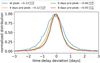 |
Fig. 12 Evaluation on a specific LSN Ia system at zs = 0.76 with (κ1,γ1, s1) = (0.25, 0.27, 0.6) for image one and (κ2,γ2, s2) = (0.83, 0.81, 0.6) for image two as in Huber et al. (2022) for at peak detection and three cases where the first SN image is detected before peak (in observer-frame days). The light curves are simulated in the same way as those in the SNEMO15-only test set. As was expected, the precision drops with less available data points pre-peak, but the uncertainty of ∼0.7 day for at-peak detection is still good. The accuracy is worse than in Fig. 9, which shows that the spread presented there is not only due to various noise and microlensing configurations but also comes from different types of LSNe Ia, although the bias cancels out if a large variety of systems is investigated. |
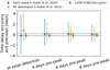 |
Fig. 13 The LSTM-FCNN in comparison to the RF developed in Huber et al. (2022) and PyCS used in Huber et al. (2019). The exact values are listed in Table 3. In terms of precision, the LSTM-FCNN outperforms the other two approaches by roughly a factor of three. |
Time-delay deviations of the LSTM-FCNN on SNEMO15- only test sets in comparison to the RF and PyCS for a LSN Ia with (κ1,γ1, s1) = (0.25, 0.27, 0.6) for image one and (κ2,γ2, s2) = (0.83, 0.81, 0.6) for image two for zs = 0.76 and various detection times (in observer days) before the first SN image peaks in brightness.
6 Summary
In this work we developed a LSTM-FCNN to measure time delays of LSNe Ia which we expect to detect with LSST and for which we plan to trigger follow-up observations. With i-band only to a mean single-epoch 5σ depth of 24.5, we can achieve over a broad sample of LSNe Ia a bias free time-delay measurement with a precision of ∼0.7 days. Our LSTM-FCNN is general and can be applied to a variety of LSNe Ia expected from LSST with subsequent dedicated follow-up monitoring. In comparison to the RF developed in Huber et al. (2022) or PyCS used in Huber et al. (2019) we see a significant improvement in precision of roughly a factor of three.
Because of the much better performance of the LSTM- FCNN in comparison to PyCS, we can expect more LSNe Ia with well measured time delay (accuracy better than 1% and precision better than 5%) than that predicted by Huber et al. (2019). For the 10-year LSST survey with a baseline observing strategy, Huber et al. (2019) predict about 28 LSNe Ia with well measured timedelay (follow-up with two day cadence and LSST-like plus one 5σ depth), out of 73 LSNe Ia systems in total. Since ∼30% are dropped due to bad accuracy from the total number of LSNe Ia (Huber et al. 2019), we can expect that any new time-delay measurement method with significantly improved precision would increase the number of LSNe Ia with well measured time delays by up to a factor of ~1.8 (= 73 ⋅ 0.7/28) in comparison to PyCS, which will be partly achieved by the LSTM-FCNN given that it is roughly three to four times more precise than PyCS.
Although we saw that our LSTM-FCNN performs much better than the RF on a large sample of LSNe Ia for which the RF would require a training process for each observation separately, our developed network cannot be blindly applied to any LSNe Ia. If follow-up strategies deviate from our assumptions (e.g., detection, filter, cadence) in Table 1, a new LSTM-FCNN needs to be trained. In particular, for light curves with cadences longer than 3 days, which are not in the training set, significant biases in the inferred time delays could arise (Appendix B). The current LSTM-FCNN is thus not well suited for lensed SNe Ia systems where the sampling is sparse, such as for SNH0pe (Frye et al. 2024) and SN Encore (Pierel et al. 2024b). Methods that make direct use of SN Ia light curve templates (e.g., Pierel & Rodney 2019; Pierel et al. 2024a) are better suited for such sparse light curves. Our LSTM-FCNN is well suited for light curves with cadences more rapid than 3 days, which are achievable with dedicated monitoring. In addition, we see from Table 1 that we assumed only positive time delays, meaning that image one should be correctly identified as the first appearing image and image two as the second one. In practice this is not a problem as always both orders can be tested and the higher time delay should be picked as the correct one given that inputs in the wrong order will provide a time delay very close to zero.
The LSTM-FCNN is a very promising approach to measure time delays in LSNe. However, so far the method presented in this work is only applicable for SNe Ia with i-band light curves. While the i band is expected to be the optimal band for most of lensed SNe Ia discovered from LSST in terms of measuring time delays (Huber et al. 2022), additional bands are useful particularly to mitigate potential chromatic microlensing effects. It will be interesting in the future to develop methods based on the LSTM-FCNN which can be applied to any kind of LSNe with any number of wavelength bands, from upcoming surveys such as the Wide Field Survey telescope (Wang et al. 2023) and the Roman Space Telescope (Spergel et al. 2015; Rose et al. 2021), in addition to the LSST (Ivezic et al. 2019).
Acknowledgements
We thank Laura Leal-Taixé, Tim Meinhardt and Yiping Shu for useful discussion, and the anonymous referee for constructive comments that improved our paper. S.H. and S.H.S. thank the Max Planck Society for support through the Max Planck Research Group and Max Planck Fellowship for S.H.S.. This project has received funding from the European Research Council (ERC) under the European Union’s Horizon 2020 research and innovation programme (grant agreement No 771776). This research is supported in part by the Excellence Cluster ORIGINS which is funded by the Deutsche Forschungsge- meinschaft (DFG, German Research Foundation) under Germany’s Excellence Strategy – EXC-2094 – 390783311.
Appendix A Photometric uncertainties
The photometric uncertainty σX(t) used in Eq. (3) is defined as:
 (A.1)
(A.1)
and
![Mathematical equation: $\sigma _{{\rm{rand }}}^2(t) = \left[ {\left( {0.04 - {\gamma ^c}} \right)x(t) + {\gamma ^c}{x^2}(t)} \right]\,\,{\rm{ma}}{{\rm{g}}^2}.$](/articles/aa/full_html/2024/12/aa49952-24/aa49952-24-eq55.png) (A.2)
(A.2)
The parameter γc varies dependent on the filter from 0.037 to 0.040 and takes the value 0.039 for the i band. Further,  , where mAB,X is the AB magnitude in filter X from Eq. (2) of the SN data point and m5 (t) is the 5σ point-source depth (for more details see LSST Science Collaboration (2009), Sec. 3.5, p. 67). The time varying 5σ point-source depth comes from the moon phase, as is presented in Huber et al. (2022).
Appendix B Different cadences
Fig. B.1 shows the application of the LSTM-FCNN to five SNEMO15-only test sets with a fixed cadence of 1, 2, 3, 4, and 6 days. While the bias is negligible for cadences that are part of the training data (1, 2, or 3 days), the precision degrades when moving from a cadence of 1 to 3 days. Furthermore, we observe that the LSTM-FCNN should not be applied to cadences that were not part of the training data.
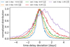 |
Fig. B.1 The LSTM-FCNN evaluated on SNEMO15-only test sets simulated as in Table 1 but with a fixed cadence of 1, 2, 3, 4, and 6 days instead of the randomly picked cadence (1, 2, or 3 days) for each sample of the training set. |
Appendix C SALT3 test set
In this section, we applied the LSTM-FCNN to a dataset based on 50,000 LSN Ia systems where the light curves are produced using the SALT3 (Kenworthy et al. 2021) model, which has never been used in the training process. For the SALT3 model, we used the asymmetric Gaussian distributions of x1 (stretch) and c (color population) as parameterized in Table 1 (all investigated surveys) by Scolnic & Kessler (2016). This parameterization matches well with the distributions shown in Fig. 4 presented by Kenworthy et al. (2021). Following Richardson et al. (2014), we assumed for the absolute B band magnitude MB = −19.25 ± 0.2 (normally distributed). To make the test even harder, instead of following parameters in Table 1, we drew time delays, κ, and γ from the OM10 sample, where we considered only the effect of macrolensing. While the macrolensing magnification is incorporated in our variety of different microlensing magnifications, as shown in Fig. 3, it is interesting to test for potential biases. The application of the LSTM-FCNN is presented in Fig. C.1, where we see a small bias in comparison to Fig. 9. However, given the substantial changes we made to the test set, this is not surprising. Importantly, the bias is still negligible if we focus on LSNe Ia systems with delays longer than 16 days, to achieve an accuracy better than 1%.
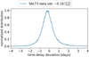 |
Fig. C.1 The LSTM-FCNN evaluated on a SALT3 dataset that was never used in the training process. |
References
- Abbott, B. P., Abbott, R., Abbott, T. D., et al. 2017, Nature, 551, 85 [Google Scholar]
- Anand, G. S., Riess, A. G., Yuan, W., et al. 2024, ApJ, 966, 89 [NASA ADS] [CrossRef] [Google Scholar]
- Arendse, N., Dhawan, S., Sagués Carracedo, A., et al. 2024, MNRAS, 531, 3509 [NASA ADS] [CrossRef] [Google Scholar]
- Bag, S., Kim, A. G., Linder, E. V., & Shafieloo, A. 2021, ApJ, 910, 65 [NASA ADS] [CrossRef] [Google Scholar]
- Bag, S., Huber, S., Suyu, S. H., et al. 2024, A&A, 691, A100 [NASA ADS] [CrossRef] [EDP Sciences] [Google Scholar]
- Balkenhol, L., et al. 2021, Phys. Rev. D, 104, 083509 [NASA ADS] [CrossRef] [Google Scholar]
- Barnabè, M., Czoske, O., Koopmans, L. V. E., Treu, T., & Bolton, A. S. 2011, MNRAS, 415, 2215 [Google Scholar]
- Bayer, J., Huber, S., Vogl, C., et al. 2021, A&A, 653, A29 [NASA ADS] [CrossRef] [EDP Sciences] [Google Scholar]
- Bessell, M., & Murphy, S. 2012, PASP, 124, 140 [NASA ADS] [CrossRef] [Google Scholar]
- Birrer, S., Treu, T., Rusu, C. E., et al. 2019, MNRAS, 484, 4726 [Google Scholar]
- Birrer, S., Shajib, A., Galan, A., et al. 2020, A&A, 643, A165 [NASA ADS] [CrossRef] [EDP Sciences] [Google Scholar]
- Blakeslee, J. P., Jensen, J. B., Ma, C.-P., Milne, P. A., & Greene, J. E. 2021, ApJ, 911, 65 [NASA ADS] [CrossRef] [Google Scholar]
- Bonvin, V., Tewes, M., Courbin, F., et al. 2016, A&A, 585, A88 [NASA ADS] [CrossRef] [EDP Sciences] [Google Scholar]
- Bonvin, V., Chan, J. H. H., Millon, M., et al. 2018, A&A, 616, A183 [NASA ADS] [CrossRef] [EDP Sciences] [Google Scholar]
- Breiman, L., 2001, Mach. Learn., 45, 5 [Google Scholar]
- Bromley, J., Bentz, J. W., Bottou, L., et al. 1993, Int. J. Pattern Recog. Artif. Intell., 07, 669 [CrossRef] [Google Scholar]
- Chan, J. H. H., Rojas, K., Millon, M., et al. 2021, A&A, 647, A115 [NASA ADS] [CrossRef] [EDP Sciences] [Google Scholar]
- Chen, G. C.-F., Fassnacht, C. D., Suyu, S. H., et al. 2019, MNRAS, 490, 1743 [NASA ADS] [CrossRef] [Google Scholar]
- Chen, W., Kelly, P. L., Frye, B. L., et al. 2024, arXiv e-prints [arXiv:2403.19029] [Google Scholar]
- Courbin, F., Bonvin, V., Buckley-Geer, E., et al. 2018, A&A, 609, A71 [NASA ADS] [CrossRef] [EDP Sciences] [Google Scholar]
- Csörnyei, G., Vogl, C., Taubenberger, S., et al. 2023, A&A, 672, A129 [NASA ADS] [CrossRef] [EDP Sciences] [Google Scholar]
- Denissenya, M., & Linder, E. V. 2022, MNRAS, 515, 977 [NASA ADS] [CrossRef] [Google Scholar]
- Denzel, P., Coles, J. P., Saha, P., & Williams, L. L. R. 2021, MNRAS, 501, 784 [Google Scholar]
- Dessart, L., & Hillier, D. J. 2005, A&A, 437, 667 [NASA ADS] [CrossRef] [EDP Sciences] [Google Scholar]
- Ding, X., Liao, K., Birrer, S., et al. 2021, MNRAS, 504, 5621 [NASA ADS] [CrossRef] [Google Scholar]
- Di Valentino, E., Mena, O., Pan, S., et al. 2021, Class. Quant. Grav., 38, 153001 [NASA ADS] [CrossRef] [Google Scholar]
- Dutcher, D., Balkenhol, L., Ade, P. A. R., et al. 2021, Phys. Rev. D, 104, 022003 [NASA ADS] [CrossRef] [Google Scholar]
- Falco, E. E., Gorenstein, M. V., & Shapiro, I. I. 1985, ApJ, 289, L1 [Google Scholar]
- Foxley-Marrable, M., Collett, T. E., Vernardos, G., Goldstein, D. A., & Bacon, D. 2018, MNRAS, 478, 5081 [NASA ADS] [CrossRef] [Google Scholar]
- Freedman, W. L. 2021, ApJ, 919, 16 [NASA ADS] [CrossRef] [Google Scholar]
- Freedman, W. L., Madore, B. F., Hatt, D., et al. 2019, arXiv e-prints [arXiv:1907.05922] [Google Scholar]
- Freedman, W. L., Madore, B. F., Hoyt, T., et al. 2020, ApJ, 891, 57 [Google Scholar]
- Frye, B. L., Pascale, M., Pierel, J., et al. 2024, ApJ, 961, 171 [NASA ADS] [CrossRef] [Google Scholar]
- Gayathri, V., Healy, J., Lange, J., et al. 2021, ApJ, 908, L34 [NASA ADS] [CrossRef] [Google Scholar]
- Goldstein, D. A., & Nugent, P. E. 2017, ApJ, 834, L5 [Google Scholar]
- Goldstein, D. A., Nugent, P. E., Kasen, D. N., & Collett, T. E. 2018, ApJ, 855, 22 [NASA ADS] [CrossRef] [Google Scholar]
- Goobar, A., Amanullah, R., Kulkarni, S. R., et al. 2017, Science, 356, 291 [Google Scholar]
- Goobar, A. A., Johansson, J., Dhawan, S., et al. 2022, Transient Name Server AstroNote, 180, 1 [NASA ADS] [Google Scholar]
- Hochreiter, S., & Schmidhuber, J. 1997, Neural Comput., 9, 1735 [CrossRef] [Google Scholar]
- Huber, S., Suyu, S. H., Noebauer, U. M., et al. 2019, A&A, 631, A161 [NASA ADS] [CrossRef] [EDP Sciences] [Google Scholar]
- Huber, S., Suyu, S. H., Noebauer, U. M., et al. 2021, A&A, 646, A110 [NASA ADS] [CrossRef] [EDP Sciences] [Google Scholar]
- Huber, S., Suyu, S. H., Ghoshdastidar, D., et al. 2022, A&A, 658, A157 [NASA ADS] [CrossRef] [EDP Sciences] [Google Scholar]
- Ivezic, Ž., Kahn, S. M., Tyson, J. A., et al. 2019, ApJ, 873, 111 [NASA ADS] [CrossRef] [Google Scholar]
- Kasen, D., Thomas, R. C., & Nugent, P. 2006, ApJ, 651, 366 [NASA ADS] [CrossRef] [Google Scholar]
- Kelly, P., Zitrin, A., Oguri, M., et al. 2022, Transient Name Server AstroNote, 169, 1 [NASA ADS] [Google Scholar]
- Kenworthy, W. D., Jones, D. O., Dai, M., et al. 2021, ApJ, 923, 265 [NASA ADS] [CrossRef] [Google Scholar]
- Khetan, N., Izzo, L., Branchesi, M., et al. 2021, A&A, 647, A72 [NASA ADS] [CrossRef] [EDP Sciences] [Google Scholar]
- Kingma, D. P., & Ba, J. 2014, arXiv e-prints [arXiv:1412.6980] [Google Scholar]
- Kourkchi, E., Tully, R. B., Anand, G. S., et al. 2020, ApJ, 896, 3 [NASA ADS] [CrossRef] [Google Scholar]
- Kromer, M., & Sim. 2009, MNRAS, 398, 1809 [CrossRef] [Google Scholar]
- Li, S., Riess, A. G., Casertano, S., et al. 2024, ApJ., 966, 20 [NASA ADS] [CrossRef] [Google Scholar]
- Lochner, M., Scolnic, D. M., Awan, H., et al. 2018, arXiv e-prints [arXiv:1812.00515] [Google Scholar]
- Lochner, M., Dan, S., Husni, A., et al. 2022, ApJS, 259, 58 [NASA ADS] [CrossRef] [Google Scholar]
- LSST Science Collaboration 2009, arXiv e-prints [arXiv:0912.0201] [Google Scholar]
- Maas, A. L., Hannun, A. Y., & Ng, A. Y. 2013, in ICML Workshop on Deep Learning for Audio, Speech and Language Processing, 30, 3 [Google Scholar]
- Millon, M., Courbin, F., Bonvin, V., et al. 2020a, A&A, 642, A193 [NASA ADS] [CrossRef] [EDP Sciences] [Google Scholar]
- Millon, M., Galan, A., Courbin, F., et al. 2020b, A&A, 639, A101 [NASA ADS] [CrossRef] [EDP Sciences] [Google Scholar]
- Mueller, J., & Thyagarajan, A. 2016, Proc. AAAI Conf. Artificial Intell., 30, 1 [Google Scholar]
- Mukherjee, S., Wandelt, B. D., Nissanke, S. M., & Silvestri, A. 2021, Phys. Rev. D, 103, 043520 [CrossRef] [Google Scholar]
- Nix, D., & Weigend, A. 1994, Proc. IEEE Int. Conf. Neural Netw., 1, 55 [Google Scholar]
- Nomoto, K., Thielemann, F.-K., & Yokoi, K. 1984, ApJ, 286, 644 [NASA ADS] [CrossRef] [Google Scholar]
- Oguri, M., & Kawano, Y. 2003, MNRAS, 338, L25 [NASA ADS] [CrossRef] [Google Scholar]
- Oguri, M., & Marshall, P. J. 2010, MNRAS, 405, 2579 [NASA ADS] [Google Scholar]
- Pakmor, R., Kromer, M., Taubenberger, S., et al. 2012, ApJ, 747, L10 [NASA ADS] [CrossRef] [Google Scholar]
- Pascale, M., Frye, B. L., Pierel, J. D. R., et al. 2024, arXiv e-prints [arXiv:2403.18902] [Google Scholar]
- Pascanu, R., Mikolov, T., & Bengio, Y. 2013, Int. Conf. Mach. Learn., 28, 1310 [Google Scholar]
- Paszke, A., Gross, S., Massa, F., et al. 2019, in Advances in Neural Information Processing Systems 32, eds. H. Wallach, H. Larochelle, A. Beygelzimer, et al. (New York: Curran Associates, Inc.), 8024 [Google Scholar]
- Pesce, D. W., Braatz, J. A., Reid, M. J., et al. 2020, ApJ, 891, L1 [Google Scholar]
- Philipp, G., Song, D. X., & Carbonell, J. G. 2018, arXiv e-prints [arXiv:1712.05577] [Google Scholar]
- Pierel, J. D. R., & Rodney, S. 2019, ApJ, 876, 107 [NASA ADS] [CrossRef] [Google Scholar]
- Pierel, J. D. R., Rodney, S., Vernardos, G., et al. 2021, ApJ, 908, 190 [NASA ADS] [CrossRef] [Google Scholar]
- Pierel, J. D. R., Arendse, N., Ertl, S., et al. 2023, ApJ, 948, 115 [NASA ADS] [CrossRef] [Google Scholar]
- Pierel, J. D. R., Frye, B. L., Pascale, M., et al. 2024a, ApJ, 967, 50 [NASA ADS] [CrossRef] [Google Scholar]
- Pierel, J. D. R., Newman, A. B., Dhawan, S., et al. 2024b, ApJ, 967, L37 [NASA ADS] [CrossRef] [Google Scholar]
- Planck Collaboration VI. 2020, A&A, 641, A6 [NASA ADS] [CrossRef] [EDP Sciences] [Google Scholar]
- Polletta, M., Nonino, M., Frye, B., et al. 2023, A&A, 675, L4 [NASA ADS] [CrossRef] [EDP Sciences] [Google Scholar]
- Quimby, R. M., Oguri, M., More, A., et al. 2014, Science, 344, 396 [NASA ADS] [CrossRef] [Google Scholar]
- Refsdal, S. 1964, MNRAS, 128, 307 [NASA ADS] [CrossRef] [Google Scholar]
- Richardson, D., III, R. L. J., Wright, J., & Maddox, L. 2014, AJ, 147, 118 [NASA ADS] [CrossRef] [Google Scholar]
- Riess, A. G., Casertano, S., Yuan, W., et al. 2018, ApJ, 861, 126 [NASA ADS] [CrossRef] [Google Scholar]
- Riess, A. G., Casertano, S., Yuan, W., Macri, L. M., & Scolnic, D. 2019, ApJ, 876, 85 [Google Scholar]
- Riess, A. G., Casertano, S., Yuan, W., et al. 2021, ApJ, 908, L6 [NASA ADS] [CrossRef] [Google Scholar]
- Riess, A. G., Yuan, W., Macri, L. M., et al. 2022, ApJ, 934, L7 [NASA ADS] [CrossRef] [Google Scholar]
- Riess, A. G., Anand, G. S., Yuan, W., et al. 2024, ApJ, 962, L17 [NASA ADS] [CrossRef] [Google Scholar]
- Rodney, S. A., Patel, B., Scolnic, D., et al. 2015, ApJ, 811, 70 [NASA ADS] [CrossRef] [Google Scholar]
- Rodney, S. A., Brammer, G. B., Pierel, J. D. R., et al. 2021, Nat. Astron., 5, 1118 [NASA ADS] [CrossRef] [Google Scholar]
- Rose, B. M., Baltay, C., Hounsell, R., et al. 2021, arXiv e-prints [arXiv:2111.03081] [Google Scholar]
- Rusu, C. E., Wong, K. C., Bonvin, V., et al. 2020, MNRAS, 498, 1440 [Google Scholar]
- Sak, H., Senior, A., & Beaufays, F. 2014, arXiv e-prints [arXiv:1402.1128] [Google Scholar]
- Saunders, C., Aldering, G., Antilogus, P., et al. 2018, ApJ, 869, 167 [NASA ADS] [CrossRef] [Google Scholar]
- Schmidt, B. P., Suntzeff, Nicholas B., et al. 1998, ApJ, 507, 46 [NASA ADS] [CrossRef] [Google Scholar]
- Schneider, P., & Sluse, D. 2014, A&A, 564, A103 [NASA ADS] [CrossRef] [EDP Sciences] [Google Scholar]
- Schöneberg, N., Abellán, G. F., Sánchez, A. P., et al. 2022, Phys. Rep., 984, 1 [CrossRef] [Google Scholar]
- Scolnic, D., & Kessler, R. 2016, ApJ, 822, L35 [Google Scholar]
- Seitenzahl, I. R., Ciaraldi-Schoolmann, F., Röpke, F. K., et al. 2013, MNRAS, 429, 1156 [NASA ADS] [CrossRef] [Google Scholar]
- Shajib, A. J., Treu, T., & Agnello, A. 2018, MNRAS, 473, 210 [Google Scholar]
- Shajib, A., Birrer, S., Treu, T., et al. 2020, MNRAS, 494, 6072 [NASA ADS] [CrossRef] [Google Scholar]
- Sherstinsky, A. 2020, Phys. D Nonlinear Phenom., 404, 132306 [NASA ADS] [CrossRef] [Google Scholar]
- Sim, S. A., Röpke, F. K., Hillebrandt, W., et al. 2010, ApJ, 714, L52 [Google Scholar]
- Sluse, D., Rusu, C. E., Fassnacht, C. D., et al. 2019, MNRAS, 490, 613 [NASA ADS] [CrossRef] [Google Scholar]
- Spergel, D., Gehrels, N., Baltay, C., et al. 2015, ArXiv e-prints [arXiv:1503.03757] [Google Scholar]
- Suyu, S. H., Bonvin, V., Courbin, F., et al. 2017, MNRAS, 468, 2590 [Google Scholar]
- Suyu, S. H., Huber, S., Cañameras, R., et al. 2020, A&A, 644, A162 [NASA ADS] [CrossRef] [EDP Sciences] [Google Scholar]
- Tewes, M., Courbin, F., & Meylan, G. 2013, A&A, 553, A120 [NASA ADS] [CrossRef] [EDP Sciences] [Google Scholar]
- Treu, T., Agnello, A., Baumer, M. A., et al. 2018, MNRAS, 481, 1041 [NASA ADS] [CrossRef] [Google Scholar]
- Vernardos, G., & Fluke, C. J. 2014, Astron. Comput., 6, 1 [Google Scholar]
- Vernardos, G., Fluke, C. J., Bate, N. F., & Croton, D. 2014, ApJS, 211, 16 [NASA ADS] [CrossRef] [Google Scholar]
- Vernardos, G., Fluke, C. J., Bate, N. F., Croton, D., & Vohl, D. 2015, ApJS, 217, 23 [CrossRef] [Google Scholar]
- Vogl, C., Sim, S. A., Noebauer, U. M., Kerzendorf, W. E., & Hillebrandt, W. 2019, A&A, 621, A29 [NASA ADS] [CrossRef] [EDP Sciences] [Google Scholar]
- Vogl, C., Kerzendorf, W. E., Sim, S. A., et al. 2020, A&A, 633, A88 [NASA ADS] [CrossRef] [EDP Sciences] [Google Scholar]
- Wang, T., Liu, G., Cai, Z., et al. 2023, Sci. China Phys. Mech. Astron., 66, 109512 [NASA ADS] [CrossRef] [Google Scholar]
- Weisenbach, L., Schechter, P. L., & Pontula, S. 2021, ApJ, 922, 70 [NASA ADS] [CrossRef] [Google Scholar]
- Weisenbach, L., Collett, T., Sainz de Murieta, A., et al. 2024, arXiv e-prints [arXiv:2403.03264] [Google Scholar]
- Wojtak, R., Hjorth, J., & Gall, C. 2019, MNRAS, 487, 3342 [Google Scholar]
- Wong, K. C., Suyu, S.H., Chen, G. C.-F et al. 2020, MNRAS, 498, 1420 [NASA ADS] [CrossRef] [Google Scholar]
- Yahalomi, D. A., Schechter, P. L., & Wambsganss, J. 2017, arXiv e-prints [arXiv:1711.07919] [Google Scholar]
- Yildirim, A., van den Bosch, R. C. E., van de Ven, G., et al. 2017, MNRAS, 468, 4216 [NASA ADS] [CrossRef] [Google Scholar]
- Yildirim, A., Suyu, S. H., & Halkola, A. 2020, MNRAS, 493, 4783 [NASA ADS] [CrossRef] [Google Scholar]
Lensing is always achromatic, meaning independent of wavelength; however the wavelength dependent spatial distribution of the SN radiation will lead to chromatic effects.
See e.g., Fig. 1 in Huber et al. (2021).
The Hadamard product is an element-wise product for two matrices of the same dimension.
To implement this, the PyTorch functions torch.nn.utils.rnn. pad_sequence, torch.nn.utils.rnn.pack_padded_sequence, and torch.nn.utils.rnn.pad_packed_sequence are used.
All Tables
Summary of our inputs for the LSTM dataset used for training, validation, and testing.
Description of the training, validation, test, and SNEMO15-only test set used in this work.
Time-delay deviations of the LSTM-FCNN on SNEMO15- only test sets in comparison to the RF and PyCS for a LSN Ia with (κ1,γ1, s1) = (0.25, 0.27, 0.6) for image one and (κ2,γ2, s2) = (0.83, 0.81, 0.6) for image two for zs = 0.76 and various detection times (in observer days) before the first SN image peaks in brightness.
All Figures
|
Fig. 1 Four random samples of our training set, comparing data without normalization (left panels) and data with normalization (right panels) that will be used for our machine-learning network. The red and blue data points are the i-band light curves for the first and the second, respectively, lensed SN image. The black curves in the left panels show the i-band 5σ limiting depth, which oscillates with the moon phase. The normalization procedure to obtain the right panels from the left panels is described in Sect. 2.2. |
| In the text | |
|
Fig. 2 Convergence κ and shear γ (upper panel), and source redshift zs and lens redshift zd (lower panel) used for the calculation of microlensed light curves drawn from the OM10 catalog. The black lines represent contours that enclose 68% of the LSN Ia systems in the OM10 catalog. |
| In the text | |
|
Fig. 3 Distribution of magnification factors from the six microlensed magnification maps under investigation in this work (solid colored), in comparison to all macro-magnification factors from all LSNe Ia from the OM10 catalog (dashed black). Microlensing magnification maps investigated in this work cover a much broader range of potential magnification factors in comparison to the macrolensing only case from the whole OM10 sample. |
| In the text | |
|
Fig. 4 i band light curves for typical source redshifts of LSNe Ia as indicated on the top of each panel. We compare four theoretical models (merger, N100, sub-Ch, and W7) with the empirical SNEMO15 model. |
| In the text | |
|
Fig. 5 Illustration of an RNN. The input xk is used to calculate state Ak of the network at the k-th time step, by using also the information from the previous k − 1 time step. The output hk is then computed from the state Ak. See Eqs. (9) and (10). |
| In the text | |
|
Fig. 6 Illustration of an LSTM. The input xk is used in combinations with the output hk−1 and the cell state ck−1 from the previous time step k − 1 to produce the output hk for the k-th time step. The cell state ck acts as memory and transports information through the cell, where the forget gate fk , input gate ik , and gate gk update information in the cell state. The output gate, based on the previous output hk−1 and input xk in combination with information from the cell state provides the new output hk. For more information, see Eqs. (11)–(16). |
| In the text | |
|
Fig. 7 Illustration of our LSTM-FCNN composed of a Siamese LSTM network and a FCNN with two hidden layers. Details about the LSTM cells are shown in Fig. 6. Both sub-LSTM networks for image one (top, input denoted by S 1k) and image two (bottom, input denoted by S2k) are the same LSTM network (i.e., with the same weights in the neural network) composed of 2 layers (LSTM A and LSTM B) where during the training process, a dropout rate of 20% is used. We use only the last outputs |
| In the text | |
|
Fig. 8 Training and validation loss of the LSTM-FCNN as a function of the training epoch. The vertical line marks the state at which we use the LSTM-FCNN where the validation loss is the lowest with the additional requirement that the bias is lower than 0.05 day. The plot shows that with more training epochs the network improves its performance while around epoch 22 000 the validation loss starts to increase again while the training loss still decreases because the LSTM-FCNN starts to overfit, meaning that, for example, it fits to specific noise patterns present in the training set. |
| In the text | |
|
Fig. 9 Evaluation of the LSTM-FCNN on the training set, validation set, test set, and SNEMO15-only test set. With a 1σ spread of ∼0.7 days and almost no bias even on the two test sets, the LSTM-FCNN is very promising for future measurements of time delays from real LSNe Ia. |
| In the text | |
|
Fig. 10 Application of the LSTM-FCNN to the validation set. The distribution shows the time-delay deviation of each sample over the predicted uncertainty of the network. In blue we see a fit with a normal distribution. |
| In the text | |
|
Fig. 11 Based on Fig. 10 we can define confidence intervals and find based on the fit function f a correction factor that needs to be applied to the predicted uncertainty of the network σpred. |
| In the text | |
|
Fig. 12 Evaluation on a specific LSN Ia system at zs = 0.76 with (κ1,γ1, s1) = (0.25, 0.27, 0.6) for image one and (κ2,γ2, s2) = (0.83, 0.81, 0.6) for image two as in Huber et al. (2022) for at peak detection and three cases where the first SN image is detected before peak (in observer-frame days). The light curves are simulated in the same way as those in the SNEMO15-only test set. As was expected, the precision drops with less available data points pre-peak, but the uncertainty of ∼0.7 day for at-peak detection is still good. The accuracy is worse than in Fig. 9, which shows that the spread presented there is not only due to various noise and microlensing configurations but also comes from different types of LSNe Ia, although the bias cancels out if a large variety of systems is investigated. |
| In the text | |
|
Fig. 13 The LSTM-FCNN in comparison to the RF developed in Huber et al. (2022) and PyCS used in Huber et al. (2019). The exact values are listed in Table 3. In terms of precision, the LSTM-FCNN outperforms the other two approaches by roughly a factor of three. |
| In the text | |
|
Fig. B.1 The LSTM-FCNN evaluated on SNEMO15-only test sets simulated as in Table 1 but with a fixed cadence of 1, 2, 3, 4, and 6 days instead of the randomly picked cadence (1, 2, or 3 days) for each sample of the training set. |
| In the text | |
|
Fig. C.1 The LSTM-FCNN evaluated on a SALT3 dataset that was never used in the training process. |
| In the text | |
Current usage metrics show cumulative count of Article Views (full-text article views including HTML views, PDF and ePub downloads, according to the available data) and Abstracts Views on Vision4Press platform.
Data correspond to usage on the plateform after 2015. The current usage metrics is available 48-96 hours after online publication and is updated daily on week days.
Initial download of the metrics may take a while.