| Issue |
A&A
Volume 658, February 2022
|
|
|---|---|---|
| Article Number | A157 | |
| Number of page(s) | 25 | |
| Section | Cosmology (including clusters of galaxies) | |
| DOI | https://doi.org/10.1051/0004-6361/202141956 | |
| Published online | 15 February 2022 | |
HOLISMOKES
VII. Time-delay measurement of strongly lensed Type Ia supernovae using machine learning⋆
1
Max-Planck-Institut für Astrophysik, Karl-Schwarzschild Str. 1, 85741 Garching, Germany
e-mail: This email address is being protected from spambots. You need JavaScript enabled to view it.
2
Technische Universität München, Physik-Department, James-Franck-Straße 1, 85748 Garching, Germany
3
Institute of Astronomy and Astrophysics, Academia Sinica, 11F of ASMAB, No. 1, Section 4, Roosevelt Road, Taipei 10617, Taiwan
4
Informatik-Department, Technische Universität München, Boltzmannstr. 3, 85748 Garching, Germany
5
Institute of Physics, Laboratory of Astrophysics, Ecole Polytechnique Fédérale de Lausanne (EPFL), Observatoire de Sauverny, 1290 Versoix, Switzerland
6
Heidelberger Institut für Theoretische Studien, Schloss-Wolfsbrunnenweg 35, 69118 Heidelberg, Germany
7
Munich Re, IT1.6.1.1, Königinstraße 107, 80802 München, Germany
8
Astrophysics Research Centre, School of Mathematics and Physics, Queen’s University Belfast, Belfast BT7 1NN, UK
Received:
5
August
2021
Accepted:
29
November
2021
Abstract
The Hubble constant (H0) is one of the fundamental parameters in cosmology, but there is a heated debate around the > 4σ tension between the local Cepheid distance ladder and the early Universe measurements. Strongly lensed Type Ia supernovae (LSNe Ia) are an independent and direct way to measure H0, where a time-delay measurement between the multiple supernova (SN) images is required. In this work, we present two machine learning approaches for measuring time delays in LSNe Ia, namely, a fully connected neural network (FCNN) and a random forest (RF). For the training of the FCNN and the RF, we simulate mock LSNe Ia from theoretical SN Ia models that include observational noise and microlensing. We test the generalizability of the machine learning models by using a final test set based on empirical LSN Ia light curves not used in the training process, and we find that only the RF provides a low enough bias to achieve precision cosmology; as such, RF is therefore preferred over our FCNN approach for applications to real systems. For the RF with single-band photometry in the i band, we obtain an accuracy better than 1% in all investigated cases for time delays longer than 15 days, assuming follow-up observations with a 5σ point-source depth of 24.7, a two day cadence with a few random gaps, and a detection of the LSNe Ia 8 to 10 days before peak in the observer frame. In terms of precision, we can achieve an approximately 1.5-day uncertainty for a typical source redshift of ∼0.8 on the i band under the same assumptions. To improve the measurement, we find that using three bands, where we train a RF for each band separately and combine them afterward, helps to reduce the uncertainty to ∼1.0 day. The dominant source of uncertainty is the observational noise, and therefore the depth is an especially important factor when follow-up observations are triggered. We have publicly released the microlensed spectra and light curves used in this work.
Key words: gravitational lensing: strong / gravitational lensing: micro / distance scale / supernovae: individual: Type Ia
© S. Huber et al. 2022
 Open Access article, published by EDP Sciences, under the terms of the Creative Commons Attribution License (https://creativecommons.org/licenses/by/4.0), which permits unrestricted use, distribution, and reproduction in any medium, provided the original work is properly cited.
Open Access funding provided by Max Planck Society.
1. Introduction
The Hubble constant, H0, is one of the fundamental parameters in cosmology, but there is a tension1 of > 4σ (Verde et al. 2019) between the early Universe measurements inferred from the cosmic microwave background (CMB; Planck Collaboration I 2020) and late Universe measurements from the Supernova H0 for the Equation of State (SH0ES) project (e.g., Riess et al. 2016, 2018, 2019, 2021). However, results from Freedman et al. (2019, 2020) using the tip of the red giant branch (TRGB) or from Khetan et al. (2021) using surface brightness fluctuations (SBFs) are consistent with both. An independent analysis using the TRGBs by Anand et al. (2021) has derived a slightly higher H0 value, bringing it closer to the results of the SH0ES project, which is based on Cepheids. Moreover, recent results from Blakeslee et al. (2021) using SBFs that are calibrated through both Cepheids and TRGBs are in good agreement with the SH0ES project and ∼2σ higher than the CMB values. As an alternative to the distance ladder approach, Pesce et al. (2020) measured H0 from the Megamaser Cosmology Project, which also agrees well with the SH0ES results and is about ∼2σ higher than the Planck value. Gravitational wave sources acting as standard sirens also provide direct luminosity distances and thus H0 measurements (e.g., Abbott et al. 2017). While this is a promising approach, current uncertainties on H0 from standard sirens preclude them from being used to discern between the SH0ES and the CMB results.
Lensing time-delay cosmography, as an independent probe, can address this tension by measuring H0 in a single step. This method, first envisaged by Refsdal (1964), combines the measured time delay from the multiple images of a variable source with lens mass modeling and line-of-sight mass structure to infer H0. The COSmological MOnitoring of GRAvItational Lenses (COSMOGRAIL; Courbin et al. 2018) and H0 Lenses in COSMOGRAIL’s Wellspring (H0LiCOW; Suyu et al. 2017) collaborations, together with the Strong lensing at High Angular Resolution Program (SHARP) (Chen et al. 2019), have successfully applied this method to lensed quasar systems (e.g., Bonvin et al. 2018; Birrer et al. 2019; Sluse et al. 2019; Rusu et al. 2020; Chen et al. 2019). The latest H0 measurement from H0LiCOW using physically motivated mass models is consistent with measurements from SH0ES but is in > 3σ tension with results from the CMB (Wong et al. 2020). The STRong-lensing Insights into the Dark Energy Survey (STRIDES) collaboration has further analyzed a new lensed quasar system (Shajib et al. 2020). The newly formed Time-Delay COSMOgraph (TDCOSMO) organization (Millon et al. 2020), consisting of H0LiCOW, COSMOGRAIL, SHARP and STRIDES, has recently considered a one-parameter extension to the mass model to allow for the mass-sheet transformation (e.g., Falco et al. 1985; Schneider & Sluse 2013; Kochanek 2020). Birrer et al. (2020) used the stellar kinematics to constrain this single parameter, resulting in an H0 value with a larger uncertainty, which is statistically consistent with the previous results using physically motivated mass models. In addition to placing constraints on H0, strongly lensed quasars also provide tests of the cosmological principle, especially of spatial isotropy, given the independent sight line and distance measurement that each lensed quasar yields (e.g., Krishnan et al. 2021a,b).
In addition to strongly lensed quasars, supernovae (SNe) lensed into multiple images are promising as a cosmological probe and are in fact the sources envisioned by Refsdal (1964). Even though these systems are much rarer in comparison to quasars, they have the advantage that SNe fade away over time, facilitating measurements of stellar kinematics of the lens galaxy (Barnabè et al. 2011; Yıldırım et al. 2017, 2020; Shajib et al. 2018) and surface brightness distributions of the lensed-SN host galaxy (Ding et al. 2021) to break model degeneracies, for example, the mass-sheet transformation (Falco et al. 1985; Schneider & Sluse 2014). Furthermore, strongly lensed type Ia supernovae (LSNe Ia) are promising given that they are standardizable candles and therefore provide an additional way to break model degeneracies for lens systems where lensing magnifications are well characterized (Oguri & Kawano 2003; Foxley-Marrable et al. 2018).
So far, only three LSNe with resolved multiple images have been observed, namely SN “Refsdal” (Kelly et al. 2016a,b), a core-collapse SN at a redshift of z = 1.49, the LSN Ia iPTF16geu (Goobar et al. 2017) at z = 0.409, and AT2016jka (Rodney et al. 2021) at z = 1.95, which is most likely a LSN Ia. Nonetheless, with the upcoming Rubin Observatory Legacy Survey of Space and Time (LSST; Ivezic et al. 2019), we expect to find ∼103 LSNe, of which 500 to 900 are expected to be type Ia SNe (Quimby et al. 2014; Goldstein & Nugent 2017; Goldstein et al. 2018; Wojtak et al. 2019). Considering only LSNe Ia with spatially resolved images and peak brightnesses2 brighter than 22.6 in the i band, as in the Oguri & Marshall (2010, hereafter OM10) lens catalog, leads to 40 to 100 LSNe Ia, depending on the LSST observing strategy, of which 10 to 25 systems yield accurate time-delay measurements (Huber et al. 2019).
To measure time delays between multiple images of LSNe Ia, Huber et al. (2019) used the free-knot spline estimator from Python Curve Shifting (PyCS; Tewes et al. 2013; Bonvin et al. 2016), and therefore the characteristic light-curve shape of a SN Ia is not taken into account. Furthermore, they do not explicitly model the variability due to microlensing (Chang & Refsdal 1979; Irwin et al. 1989; Wambsganss 2006; Mediavilla et al. 2016), an effect where each SN image is separately influenced by lensing effects from stars in the lens, leading to the additional magnification and distortion of light curves (Yahalomi et al. 2017; Goldstein et al. 2018; Foxley-Marrable et al. 2018; Huber et al. 2019, 2021; Pierel & Rodney 2019). While PyCS has the advantage of being flexible without making assumptions on the light-curve forms, model-based methods are complementary in providing additional information to measure the time delays more precisely.
One such model-based time-delay measurement method was implemented by Pierel & Rodney (2019), where template SN light curves are used. Even though microlensing is taken into account in this work, it is done in the same way for each filter. A more realistic microlensing treatment for SNe Ia, with variations in the SN intensity distribution across wavelengths, was first introduced by Goldstein et al. (2018) using specific intensity profiles from the theoretical W7 model (Nomoto et al. 1984) calculated via the radiative transfer code SEDONA (Kasen et al. 2006). Huber et al. (2019, 2021) have built upon this study, but using the radiative transfer code ARTIS (Kromer & Sim 2009) to calculate synthetic observables for up to four theoretical SN explosion models. In this work, we follow the approach of Huber et al. (2019, 2021) to calculate realistic microlensed light curves for LSNe Ia to train a fully connected neural network (FCNN) and a random forest (RF) model for measuring time delays. In addition, this method also allows us to identify dominant sources of uncertainties and quantify different follow-up strategies.
This paper is organized as follows. In Sect. 2 we present our calculation of mock light curves, which includes microlensing and observational uncertainties. The creation of our training, validation, and test sets is explained with an example mock observation in Sect. 3, followed by an introduction to the machine learning (ML) techniques used in this work in Sect. 4. We apply these methods to the example mock observation in Sect. 5, where we also test the generalizability by using empirical LSN Ia light curves not used in the training process. In Sect. 6 we investigate, based on our example mock observation, potential filters for follow-up observations and the impact of microlensing and noise on the uncertainty, before we investigate more mock observations in Sect. 7. We discuss our results in Sect. 8 before summarizing in Sect. 9. Magnitudes in this paper are in the AB system.
We have publicly released the microlensed spectra and light curves used in this work online3.
2. Simulated light curves for LSNe Ia
The goal is to develop a software that takes photometric light-curve observations of a LSN Ia as input and predicts as an output the time delay between the different images. For a ML approach, we need to simulate a realistic data set where we account for different sources of uncertainties. We therefore specify in Sect. 2.1 our calculation of microlensing, and we explain in Sect. 2.2 our determination of observational uncertainties including estimates of the moon phase.
2.1. Microlensing and SN Ia models
To calculate light curves for a LSN Ia with microlensing, we combine magnifications maps from GERLUMPH (Vernardos & Fluke 2014; Vernardos et al. 2014, 2015) with theoretical SN Ia models, where synthetic observables have been calculated with ARTIS (Kromer & Sim 2009). The basic idea is to place a SN in a magnification map and solve for the observed flux:
 (1)
(1)
where Dlum is the luminosity distance to the source, zs is the redshift of the source, μ(x, y) is the magnification factor depending on the positions (x, y) in the magnification map, and Iλ, e(t, p) is the emitted specific intensity at the source plane as a function of wavelength, λ, time since explosion, t, and impact parameter, p (i.e., the projected distance from the ejecta center, where we assume spherical symmetry similar to Huber et al. 2019, 2021). Lensing magnification maps depend on three main parameters, namely the convergence κ, the shear γ and the smooth matter fraction s = 1 − κ*/κ, where κ* is the convergence of the stellar component. Further, our maps have a resolution of 20 000 × 20 000 pixels with a total size of 20 REin × 20 REin, where the Einstein radius, REin, is a characteristic size of the map that depends on the source redshift zs, lens redshift zd, and masses of the microlenses. As in Huber et al. (2021), we follow Chan et al. (2021) for generating the microlensing magnification maps and assume a Salpeter initial mass function (IMF) with a mean mass of the microlenses of 0.35 M⊙; the specifics of the assumed IMF have negligible impact on our studies. From the flux we obtain the AB magnitudes via
 (2)
(2)
(Bessell & Murphy 2012), where c is the speed of light and SX(λ) is the transmission function for the filter X (that can be u, g, r, i, z, y, J, or H in this work). This calculation is discussed in much greater detail by Huber et al. (2019), which was initially motivated by the work of Goldstein et al. (2018).
The calculation of microlensing of LSNe Ia requires a theoretical model for the SN Ia that predicts the specific intensity. To increase the variety of different light-curve shapes we use four SNe Ia models computed with ARTIS (Kromer & Sim 2009). These models have also been used in Suyu et al. (2020) and Huber et al. (2021), and are briefly summarized in the following: (i) the parameterized 1D deflagration model W7 (Nomoto et al. 1984) with a Chandrasekhar mass (MCh) carbon-oxygen (CO) white dwarf (WD), (ii) the delayed detonation model N100 (Seitenzahl et al. 2013) of a MCh CO WD, (iii) a sub-Chandrasekhar (sub-Ch) detonation model of a CO WD with 1.06 M⊙ (Sim et al. 2010), and (iv) a merger model of two CO WDs of 0.9 M⊙ and 1.1 M⊙ (Pakmor et al. 2012).
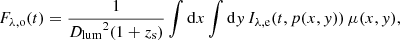
Figure 1 shows the light curves for the four SN Ia models in comparison to the empirical SNEMO15 model (Saunders et al. 2018). The light curves are normalized by the peak. Magnitude differences between SN Ia models are within 1 mag. To produce the median and 2σ (97.5th percentile – 2.5th percentile) light curves of SNEMO15, we consider all 171 SNe Ia from Saunders et al. (2018). Data of the empirical models cover only 3305 Å to 8586 Å and therefore the u band, starting at 3200 Å, is only an approximation, but an accurate one since the filter transmission in the missing region is low. The rest-frame u and g cover approximately the observed r, i, and z bands for a system with redshift of 0.76, which we investigate in Sects. 3 and 5. Light curves from theoretical and empirical models show the same evolution, although there are quite some differences in the shapes. The variety of different theoretical models is helpful to encapsulate the intrinsic variation of real SNe Ia. In building our training, validation and test sets for our ML methods, we also normalize the light curves after the calculation of the observational noise, which we describe next.
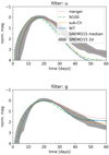 |
Fig. 1. Normalized LSST u- and g-band rest-frame light curves for four theoretical SN Ia models (merger, N100, sub-Ch, and W7) in comparison to the empirical model SNEMO15. |
2.2. Observational uncertainty and the moon phase
Magnitudes for filter X including observational uncertainties can be calculated via
 (3)
(3)
where mAB, X is the intrinsic magnitude without observational noise, rnorm is a random Gaussian number with a standard deviation of unity, and σ1, X is a quantity that depends mainly on mAB, X relative to the 5σ depth m5. This calculation is based on LSST Science Collaboration (2009) (for more details, see also Appendix A).
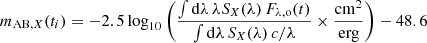
In order to calculate mdata, X, the 5σ depth of the corresponding filter X is needed. In this work we consider eight filters, namely the six LSST filters, u, g, r, i, z, and y, as well as two infrared bands, J and H. To estimate the moon phase dependence of filter X, we used the exposure time calculator (ETC) of the European Southern Observatory (ESO) with a flat template spectrum. For ugriz we used the ETC of OmegaCAM4, and for yJH we used the ETC of VIRCAM5, where we assume an airmass of 1.2. Further, we used the typical fixed sky model parameters with seeing ≤1″ as provided by the ETC, which we found to be a conservative estimate of the 5σ depth by testing other sky positions. We investigated one cycle phase (25 August 2020 to 24 September 2020) to obtain relative changes of the 5σ depth with time and matched these relative changes to the typical mean of the single-epoch LSST-like 5σ depth plus one magnitude, given by (23.3+1, 24.7+1, 24.3+1, 23.7+1, 22.8+1, and 22.0+1) for (u, g, r, i, z, and y), respectively, assuming a fixed exposure time. These mean values take into account that in typical LSST observing strategies, redder bands are preferred around full moon, while bluer bands are used more around new moon. Going one magnitude deeper than the LSST 5σ depth provides a better quality of photometric measurements for time-delay measurements, and is feasible even for a 2 m telescope (Huber et al. 2019). The absolute values for J and H bands are set by the ETC of VIRCAM in comparison to the y band.
The results for one cycle phase are shown in Fig. 2, where we find full moon around day 8 and new moon around day 23. As expected, bluer bands are much more influenced by the moon phase in comparison to redder bands. As we are typically interested in getting LSNe Ia with time delays greater than 20 days (Huber et al. 2019), it is important to take the moon phase into account. Furthermore, we note that our approach on the 5σ depth assumes an isolated point source, where in reality we also have contributions from the host and lens light, which are the lowest for faint hosts and large image separations. Even though these are the systems we are interested in targeting, our uncertainties are on the optimistic side. The construction of light curves in the presence of the lens and host is deferred to future work, although LSNe have the advantage that the SNe fade away and afterward an observation of the lensing system without the SN can be taken and used as a template for subtraction.
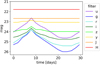 |
Fig. 2. Estimated 5σ depth for eight different filters, u, g, r, i, z, y, J, and H, accounting for the moon phase. Day 0 corresponds to the first quarter in the moon phase. Full moon is around day 8, and new moon is on day 23. |
3. Example mock observation and data set for machine learning
In this section we present a specific mock observation as an example, to explain the data structure required for our ML approaches.
3.1. Mock observation
As an example, we take a LSN Ia double system of the OM10 catalog (Oguri & Marshall 2010), which is a mock lens catalog for strongly lensed quasars and SNe. The parameters of the mock LSN Ia are given in Table 1, where we have picked a system with a source redshift close to the median source redshift zs = 0.77 of LSNe Ia in OM10 (Huber et al. 2021). The corresponding mock light curves are produced assuming the W7 model, where the i band is shown in Fig. 3 and all bands (ugrizyJH) together are shown in Appendix B. To calculate magnitudes with observational noise we use Eq. (3). For the moon phase we assume a configuration where the i-band light curve peaks around new moon. Further configurations in the moon phases will be discussed in Sect. 7.1. To avoid unrealistic noisy data points mdata, X for our mock system in Fig. 3, we only take points mAB, X brighter than m5 + 2 mag into account, before we add noise on top. Furthermore, we assume a two day cadence with a few random gaps.
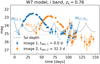 |
Fig. 3. Simulated observation for which ML models will be trained to measure the time delay. The gray dashed curve marks the 5σ point-source depth, that accounts for the moon phase. The marked data points are also listed in Eq. (4). |
Mock system of the OM10 catalog for generating mock light curves to train our ML techniques.
3.2. Data set for machine learning
Our data of the mock LSN Ia contain measurements of light curves in one or more filters of the two SN images. The input data for our ML approaches are ordered, such that for a given filter, all magnitude values from image 1 are listed (first observed to last observed), followed by all magnitude values from image 2. This structure is illustrated in the following definition and will be referred to as a single sample,
 (4)
(4)
for an example of a double LSN Ia with observations in the i band. There are Ni1 photometric measurements in the light curve for SN image 1, and Ni2 photometric measurements for SN image 2. The magnitude value of the first data point in the i band from the first image in Fig. 3 is denoted as mi1, 1, and the last data point is mi1, Ni1. The first data point of the second image in the i band is denoted as mi2, 1. For simplification, we define Nd = Ni1 + Ni2, and dj as the jth magnitude value in Eq. (4). If multiple filters are available, then a ML model can be trained per band, or multiple bands can be used for a single ML model, which will be explored in Sect. 6.3.
We introduce our FCNN and RF methods in detail in Sect. 4; we describe here the data set required for these two approaches in the remainder of this section. Important to note is that both methods always require the same input structure as defined in Eq. (4), with exactly the same number of data points6. From this input, we can then build a FCNN or a RF that predicts the time delay. As additional information, the 5σ depth is required for each data point, to create noise in a similar way as in our mock observation. Furthermore, microlensing uncertainties are taken into account by using the κ, γ, and s values of each LSN Ia image. The weakness of this approach is that we need to train a ML model for each observed LSNe Ia individually, but the advantage is that we can train our model very specifically for the observation pattern, noise and microlensing uncertainties such that we expect an accurate result with a realistic account of the uncertainties. Given that the data production and training of such a system take less than a week and multiple systems can be trained in parallel, this approach is easily able to measure the delays of the expected 40 to 100 potentially promising LSNe in the 10 year LSST survey (Huber et al. 2019).
Our ML approaches require the same number of data points in each sample. We therefore produce our data set, for training, validation and testing of the ML models, such that the number of data points is always the same as in our mock observation in Fig. 3. We calculate the light curves for the SN images via Eqs. (1) and (2) where we use random microlensing map positions. We then shift the light curves for each SN image randomly in time around a first estimate of the delay. In our example, we use the true observed time values of the mock observation tobs, 1 = 0.0 d and tobs, 2 = 32.3 d as the first estimate for the SN images 1 and 2, respectively. For a real system, we do not know these time values exactly and therefore probe a range of values around these first estimates in our training, validation and test sets. In particular, for each sample in the training set, we pick random values between tobs − 10 d and tobs + 12 d as the “ground truth” (input true time value) for that specific sample. Different samples in the training set have different ground truth values. We also tested more asymmetric ranges with tobs − 10 d and tobs + test, where test = 16, 18, 22, 30 d, and find results in very good agreement, with no dependence on asymmetries in the initial estimate.
Data points are then created at the same epochs as the initial observation. Using the 5σ depth of each data point of our observation, we calculate for each random microlensing position 10 random noise realizations following Eq. (3). Since we are not interested in the overall magnitude values we normalize the resulting light curve by its maximum. Our total data set used for training has a size of 400 000 samples coming from 4 theoretical SN Ia models, 10 000 microlensing map positions and 10 noise realizations. Each sample has the data structure of Eq. (4). For the validation and test sets, we calculate two additional microlensing maps with the same κ, γ and s values as the training set, but with different microlensing patterns from random realizations of the stars. This provides “clean” validation and test sets that the ML methods have not encountered during training in order to fairly assess the performance of the methods. Our validation and test set have each a size of 40 000 samples, from 4 models, 1000 microlensing map positions and 10 noise realizations.
Two examples of our training data are shown in Fig. 4 in open circles. The first panel (sample 5) shows for the first SN image a good match to the initial mock observation (in solid circle). The simulated training data are therefore almost the same as the mock observation. Differences in fainter regions (higher normalized magnitudes) come from observational noise. For the second image, the time value t2 of the simulated training data is larger than the true value tobs, 2 and therefore we find the peak a few data points later. The general idea of providing data in such a way is that the ML model learns to translate the location of the peak region into the time value t. The difference between the two time values from the first and second image is then the time delay we are interested in. The second panel (sample 33) in Fig. 4 is a nice example illustrating why going directly for the time delay is not working that well in this approach. We see that both simulated images for training are offset to the right by almost the same amount. This would in the end lead to a very similar time delay as the initial mock observations, even though the input values are very different from those of the initial observations.
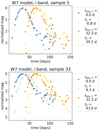 |
Fig. 4. Simulated data to train a ML model. The filled dots correspond to the mock observation shown in Fig. 3. The open dots represent the simulated training samples, where two out of the 400 000 are shown for the i band in the top and bottom panels. |
Our described approach can be seen as a fitting process that has the weakness that if the models for training are very different in comparison to a real observation, our approach will fail. From Fig. 1 we see that the four SN Ia models predict different shapes of the light curves and locations of peaks. Therefore, to compensate for different peak locations, we randomly shift the four SN Ia models in time by −5 to 5 days. Furthermore, to make the noise level more random and compensate for different peak brightness, we vary also the overall magnitude values by −0.4 to 0.4. The random shifts in time and magnitude are the same for a single sample, and therefore this approach creates basically a new model with the same light-curve shape, but slightly different peak location and brightness. Since the ML models do not know the actual values of the random shifts in time or magnitude the location of the peak for a certain SN Ia model is smeared out. Therefore, this approach introduces a much larger variety in the SN Ia models and Appendix C shows that this helps to generalize to light curves from sources that were not used in training the ML model. We also tested random multiplication factors to stretch or squeeze the light curves in time (instead of the random constant shift in time as just described), but our approach with the random shifts works slightly better as discussed in Appendix C. We therefore use the random shifts for the rest of this paper.
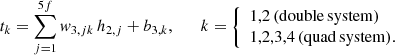
4. Machine learning techniques
In this section we explain the two different ML models used in this work, namely a deep learning network using fully connected layers and a RF. We use these simple ML approaches to get started, because if they work well, then more complicated models might not be necessary. Results from these simple approaches would also serve as a guide for the development of more complex ML models. The techniques all use the input data structure as described in Sect. 3, and provide for each image of the LSN Ia a time value t as shown in Fig. 3. For the first appearing image, the (ground truth) time t = 0 is the time of explosion and for the next appearing image it is the time of explosion plus the time delay Δt. Given our creation of the data set, which is done like a fitting process for each light curve, we do not train the system to predict only the time delay, but instead we have as output one time value per image as described in Sect. 3.2.
4.1. Deep learning – Fully connected neural network
Neural networks are a powerful tool with a broad range of applications. To solve our regression problem, we used a FCNN, consisting of an input layer, two hidden layers, and one output layer, as shown in Fig. 5. Although universal approximation results (Cybenko 1989; Hornik et al. 1989) suggest that a FCNN with only one hidden layer of arbitrarily large width can approximate any continuous function, FCNNs with finite widths but more layers have shown to be more useful in practice. We therefore used two hidden layers instead of one and tested different widths of the networks by introducing the scaling factor f for a variable number of nodes in the hidden layers in order to optimize the number of hidden nodes.
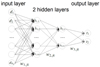 |
Fig. 5. FCNN, where the input layer has Nd data points and dj stands for the magnitude value of the jth data point in Eq. (4). The size of the two hidden layers scales by a factor f, and the outputs are two (four) time values for a double (quad) LSN Ia. |
In our FCNN, each node of the input layer corresponds to a magnitude value of a single observation for a given filter and image, sorted as in the example of Eq. (4). Each node of the input layer (dj) is connected by a weight (w1, jk) to each node of the first hidden layer (h1, k). In addition, a bias (b1, k) is assumed and we introduce non linearities, by using a rectified linear units (ReLU) activation function (e.g., Glorot et al. 2010; Maas et al. 2013), which is 0 for all negative values and the identity function for all positive values. Therefore, the nodes of the first hidden layer can be calculated via
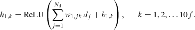 (5)
(5)
Further, all nodes in the first hidden layer are connected to all nodes in the second hidden layer in a similar manner:
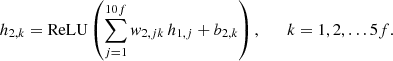 (6)
(6)
The nodes from the second hidden layer are then finally connected to the output layer to produce the time values
 (7)
(7)
The output layer consists of two nodes for a double LSN Ia and four nodes for a quad LSN Ia. We tested also other FC network structures such as using a different network for each image, using three hidden layers, or using a linear or leaky ReLU activation function, but our default approach described above works best.
We train our system for a certain number of epochs Nepoch, where we use the ML library PyTorch (Paszke et al. 2019). At each epoch, we subdivide our training data randomly into mini batches with size Nbatch. Each mini batch is propagated through our network to predict the output that we compare to the ground-truth values by using the mean squared error (MSE) loss. To optimize the loss function, we use the Adaptive Moment Estimation (Adam) algorithm (Kingma & Ba 2014) with a learning rate α on the MSE loss to update the weights in order to improve the performance of the network7. Per epoch, we calculate the MSE loss of the validation set from our FCNN, and store in the end the network at the epoch with the lowest validation loss. By selecting the epoch with the lowest validation loss, we minimize the chance of overfitting to the training data. Typically we reach the lowest validation loss around epoch 200 and an example for the training and validation curve for our FCNN is shown in Appendix D.
The test data set is used in the end to compare different FCNNs, which have been trained with different learning rates α, sizes f and mini-batch sizes Nbatch.
4.2. Random forest
The RF (Breiman 2001) is a method used for classification and regression problems, by constructing many random decision trees. In this section we give a brief introduction on the idea of a RF and explain the setup we are using.
To build a RF, we construct many random regression trees, which are a type of decision trees, where each leaf represents numeric values (for the outputs). For our case, we create a total of Ntrees random regression trees where a schematic example for a single regression tree is shown in Fig. 6. The root node is shown in magenta, the internal nodes in gray and the leaf nodes in green. The root node splits our whole data set containing samples as defined by Eq. (4), into two groups based on a certain criterion (e.g., mi1, 2 < 1.2): first where the criterion is true, and second where it is not. The internal nodes split the data in the same manner, until no further splitting is possible and we end up at a leaf node to predict the two time values t1 and t2 as output.
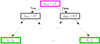 |
Fig. 6. Schematic example of a regression tree for a double system that predicts two time values for certain input data as in Eq. (4). The root node is represented by the magenta box, the internal nodes by gray boxes, and the leaf nodes by green boxes. |
To create random regression trees we use a bootstrapped data set, which draws randomly samples from the whole training data (400 000 samples) until it reaches a given size Nmax samples. Importantly, an individual sample of the original training data can be drawn multiple times and each random regression tree is built from an individual bootstrapped data set, which is used to create the root, internal and leaf nodes. However, only a random subset of the features (e.g., just mi1, 2, mi2, 5, and mi2, 9) is considered to construct the root node or a single internal node, where the splitting criterion (e.g., mi1, 2 < 0.5) of a single feature is defined based on the mean value (e.g.,  ) from all samples under investigation (Nmax samples for the root node and fewer samples for the internal nodes depending on how the data set was split before). The number of available features we pick randomly from all features for the creation of a node is Nmax features8.
In the following, we demonstrate the construction of the root node for a regression tree, as shown in Fig. 6, for the example of Nmax features = 3. Therefore, we randomly pick three features from Eq. (4), which we assume to be mi1, 2, mi2, 5, and mi2, 9. From a bootstrapped data set with Nmax samples samples of our training data set, we assume to find the mean values  ,
,  , and
, and  . Therefore, we investigate the three criteria mi1, 2 < 1.2, mi2, 5 < 1.0, and mi2, 9 < 0.6 as potential candidates for the root node, where each of the criteria splits the Nmax samples training samples into two groups. We select the best splitting criterion as the one that results in the lowest variance in the predictions within each of the groups created by the split. In other words, we can compute through this comparison a residual for t1 and t2 for each sample. From this, we can calculate the sum of squared residuals for each candidate criterion, and the criterion that predicts the lowest sum of squared residuals will be picked as our root node, which would be mi1, 2 < 1.2 in our schematic example. For each of the resulting two groups, we follow exactly the same procedure to construct internal nodes that split the data further and further until no further splitting is possible or useful9 and we end up at a leaf node to predict the output. To avoid a leaf node containing just a single training sample, we used two parameters, namely, Nmsl, the minimum number of samples required to be in a leaf node, and Nmss, the minimum number of samples required to split an internal node. From the multiple training samples in a leaf node, the t1 and t2 values of a leaf node are the average of all samples in the leaf node.
Following the above procedure, many random regression trees are built; to create an output for a single (test) sample, all regression trees are considered and the final output is created from averaging over all trees.
For this approach we used the object sklearn.ensemble.RandomForestRegressor of the software scikit-learn (Pedregosa et al. 2011; Buitinck et al. 2013), where we assume the default parameters except for the previously mentioned Nmsl, Nmss, Ntrees, Nmax samples and Nmax features.
5. Machine learning on example mock observation
In this section we apply the ML techniques from Sect. 4 to our example mock observation of a double LSNe Ia described in Sect. 3. In Sect. 5.1 we find the best FCNN and RF and compare results from the corresponding test sets based on the four theoretical models also used in the training process. In Sect. 5.2 we use the best FCNN and RF and apply it to an empirical data set not used in the training process to test the generalizability of both models. This final test is very important since in reality we can never assure that our assumed light-curve shapes in the training process will fully match a real observation.
5.1. Best fit: Fully connected neural network versus random forest
To find a FCNN and a RF that provide the best fit to our mock observation from Fig. 3, we explore a set of hyperparameters as listed in Table 2 for the FCNN and Table 3 for the RF.
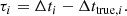
To find the best ML model for our mock observation, we used the test set to evaluate each set of hyperparameters. This is just to find an appropriate set of hyperparameters, which we will use for the sake of simplicity from here on throughout the paper10. Our final judgment of the performances of the ML models will be based on the “SNEMO15 data set” where light curves will be calculated using an empirical model (see Sect. 5.2). The distinctions between the various data sets for our ML approaches are summarized in Table 4. For each sample i of the test set, we get two time values, t1, i and t2, i, from which we can calculate the time delay Δti = t1, i − t2, i, which we compare to the true time delay Δttrue, i to calculate the “time-delay deviation” of the sample as
 (8)
(8)
Explanation of the different types of data sets used for our ML approaches.
We investigate here the absolute time-delay deviation instead of the relative one (τi/Δttrue, i), because this allows us to draw conclusions about the minimum time delay required to achieve certain goals in precision and accuracy. From our results, we do not find a dependence on the absolute time delay (e.g., 32.3 d for Fig. 4) used in the training process, which is what we expect from the setup of the FCNN and the RF and is demonstrated in Sect. 7.4.
For the FCNN, we find that (α, f, Nbatch, Nepoch) = (0.0001, 40, 256, 400) provides the best result, meaning that the median of τi of the whole test set is lower than 0.05 days (to reduce the bias) and the 84th–16th percentile (1σ credible interval) of the test set is the lowest of all networks considered. For the RF the hyperparameters  provide the best result. In the following we always use these two sets of hyperparameters for the FCNN or the RF, unless specified otherwise. We note that Ntrees = 800 is on the upper side of what we investigated, but increasing the number of trees further makes the computation even more costly. Nevertheless, we tested also Ntrees = 1000, 1200, 1600, 2000 and Ntrees = 3000 with (Nmss, Nmsl, Nmax samples, Nmax features) from the best fit as listed above. We find results that are basically the same as for Ntrees = 800 or slightly worse (0.02 d at most) and therefore we stick with Ntrees = 800, which is sufficient. The comparison between the FCNN and the RF is shown in Fig. 7, where we quote the median (50th percentile), with the 84th–50th percentile (superscript) and 16th–50th percentile (subscript) of the whole sample of light curves from the corresponding test set. The results include microlensing and observational uncertainties as described in Sect. 2. For the training and testing, we considered the four SN Ia models, merger, N100, sub-Ch and W7 (therefore we use the description “corresponding test set” in the title of Fig. 7). Further, the results are based on using just the i band, assuming the data structure as defined in Eq. (4).
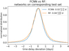 |
Fig. 7. FCNN and RF on the whole sample of light curves from the specified test set for the mock observation in Fig. 3. The ML models’ hyperparameters are set to the values at which the test set yields a bias below 0.05 days and the smallest 68% credible interval of the time-delay deviation (in Eq. (8)). |
Instead of looking at the whole sample of light curves from the test set at once, we show in Appendix E how the time-delay deviation τi depends on the time delay of the test samples. We find for both networks a slight trend that time delays far away from the true time delay of the mock observation yield larger deviations, where the effect is stronger for the RF in comparison to the FCNN. However, this is not surprising as very long time delays come from rare scenarios where the t1 value of the first image is highly underestimated and the t2 value of the second image is highly overestimated. Similarly, very short time delays tend to have t1 that is highly overestimated and t2 that is underestimated. Given that these scenarios are rare in the training set, it is more difficult to learn these cases. Still, the FCNN compensates for these edge effects better, which explains the better performance of the FCNN in comparison to the RF on the corresponding test set as shown in Fig. 7.
However, we see that both ML models provide accurate measurements of the time delay with the 1σ uncertainty for the FCNN around 0.7 days and the RF around 0.8 days, where both have low bias (≤0.04 days). Nevertheless, the training and test set is produced by using the same SN Ia models. If light curves in the test sets are different from the ones used for training, this can lead to broadened uncertainties, and more critically, also to biases (see Appendix C). Further, we learn from Appendix C that, as soon as the different light curves used for training cover a broad range, the trained ML model can be used for light-curve shapes it has never seen. Therefore, in Sect. 5.2, we evaluate the RF and the FCNN trained on four theoretical models on a data set based on the empirical SNEMO15 model.
5.2. Generalizability of ML models: Evaluation on SNEMO15 data set
To test if the ML models trained on four SN Ia models with the random shifts in time and magnitude as introduced in Sect. 3.2 can generalize well enough to real SN Ia data, we created a data set based on the empirical SNEMO15 model, which is shown in Fig. 1. The empirical model covers only a wavelength range from 3305 Å to 8586 Å, and with zs = 0.76 (Table 1), the i band is the bluest band we can calculate.
To account for macrolensing and brightness deviations for the SNEMO15 model in comparison to the theoretical SN models, we set the median SNEMO15 light curve equal to the mean value of the four macrolensed SN Ia models. Since the light curves are normalized before the training process, this is only important to avoid over- or underestimations of the observational noise. Furthermore, to include microlensing, we use microlensed light curves from the four theoretical models, initially created for the corresponding test set, and subtract the macrolensed light curve, assuming μmacro = 1/((1 − κ)2 − γ2). Therefore, we get from our 4 models 4000 microlensing contributions for the light curves, which the FCNN or the RF have not seen in its training process. For each of the microlensing contributions, we then draw randomly one of the 171 SNEMO15 light curves to create a microlensed SNEMO15 light curve. From the 4000 microlensing contributions, we have a sample of 4000 microlensed light curves. For each light curve, we then draw 10 random noise and time-delay realizations to create a data set, as described in Sect. 3.2. We call this the SNEMO15 data set.
Figure 8 shows the results where we evaluate the FCNN and the RF from Fig. 7, trained on four theoretical SN Ia models, on the corresponding test set (built from the same four theoretical SN Ia models) and on the SNEMO15 data set. The first important thing we note is that the RF shows almost no bias, whereas the FCNN has a higher bias when evaluated on the SNEMO15 data set. To investigate this further, we look at results from the RF and the FCNN for the set of hyperparameters as listed in Tables 2 and 3 for three different cases using the i band, z band, or y band.
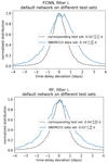 |
Fig. 8. FCNN and RF trained on four theoretical models for the i band evaluated on the whole sample of light curves from the two specified data sets. The dashed black line represents the corresponding test set based on the four theoretical models, and the data set of the blue line is based on the empirical SNEMO15 model. |
We find that the absolute bias of the FCNN for the different hyperparameters and bands (i, z, and y) is mostly below 0.4 days but higher values are also possible. The problems are that these variations in the bias in the SNEMO15 data set are not related to biases we see in the corresponding test sets or due to a specific set of hyperparameters. As a result, we cannot identify the underlying source of the bias, apart from that it is due to suboptimal generalization of the theoretical SN Ia models to SNEMO15 in the FCNN framework.
The RF works much better in this context, as the absolute bias is always lower than 0.12 days for the i, z, and y bands. Only the hyperparameter Nmax features = 1 can lead to a higher bias up to 0.22 days, but this hyperparameter is excluded because of its much worse performance in precision on the corresponding test set in comparison to  or Nmax features = Nall features. Therefore, as long as we restrict ourselves to LSNe Ia with delays longer than 12 days we can achieve a bias below 1%, which allows accurate measurements of H0. Furthermore, the bias is not the same in all filters. While the absolute bias in the y band goes up to 0.12 days, we have a maximum of 0.08 days in the z band and 0.03 days in the i band. The comparison of multiple bands therefore helps to identify some outliers.
The bias investigation of the FCNN and the RF is summarized in Fig. 9 using all hyperparameters (except Nmax features = 1, which is excluded because of its bad performance on the corresponding test set) and the i, z, and y bands. From the upper panel we see that the large biases of our FCNN on the SNEMO15 data set are not related to biases we see in the corresponding test set and therefore identifying a set of hyperparameters just from the corresponding test set which works also well on the SNEMO15 data set is not possible. From the lower panel of Fig. 9 we see that also the biases in the RF from the corresponding test set and the SNEMO15 data set are not directly related with each other but this is not a problem as the biases on the SNEMO15 data set are low enough for precision cosmology. From this example we see that the RF is able to generalize to a new kind of data not used in the training process, which does not work well for our FCNN. In principle this was already suggested by the investigation done in Appendix C, but with the random shifts in time we introduced, it seemed to significantly improve the generalizability, but it was still not enough for the final test on the SNEMO15 data set. Investigating the importance of all the input features as listed in Eq. (4), we find that the FCNN focuses mostly on the peak directly whereas for the RF the features before and after the peak are the most important ones. More about this is discussed in Appendix F.
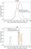 |
Fig. 9. Bias of FCNN and RF on the corresponding test set, composed of four theoretical SN Ia models used for training, and a data set based on the empirical SNEMO15 model, not used during training, for a variety of different hyperparameters and filters (i, z, and y), i.e., from model averaging. The large biases on the SNEMO15 data set up to 1 day in our FCNN approach come from the different hyperparameters even though the corresponding test set provides biases within 0.25 days. The RF provides much lower biases in all cases; it depends only weakly on the hyperparameters and is instead mostly set by the filters under consideration. |
In the remainder of the paper, we proceed to present results based on the RF, because the significant bias in our FCNN makes accurate cosmology difficult to achieve especially for LSN Ia systems with short delays. Using deeper networks would not be enough to improve our FCNN, as this would just allow a better fit to the training data but does not ensure any improvement on the generalizability of the network. Therefore, it would be necessary to provide more realistic input light curves for the training process, as it has problems to generalize to light-curve shapes it has not seen. Such an improvement could be achieved by using the SNEMO15 light curves as well in the training process, but then a test set with light-curve shapes it has never seen would be missing. Another approach would be to incorporate regularization or dropout into our FCNN or by constructing a network that outputs in addition to the time values the associated uncertainties, but given that this was not necessary for the corresponding test set to perform well, it would be some kind of fine tuning to our SNEMO15 data set, because all tests before were encouraging to proceed to the final test. Therefore, we postpone further investigations of FCNNs to future studies, especially since other network architecture, such as recurrent neural networks, long short-term memory networks (Sherstinsky 2020), or Gaussian processes, could potentially reduce model complexity while having lower inductive bias11 (Wilson & Izmailov 2020).
Another thing we learn is that the distribution of the recovered time delays from the SNEMO15 data set is ∼0.5 days broader than that of the corresponding test sets. This is not surprising as the RF and the FCNN have never seen such light curves in the training process. A ∼1.4 day precision on a single LSN Ia is still a very good measurement and allows us to conduct precision cosmology from a larger sample of LSNe Ia. Nevertheless, we see in this section that even though the uncertainties for the RF are larger than that of the FCNN, the RF provides low bias when used on empirical data and is therefore preferred.
6. Microlensing, noise, and choice of filters
In this section we use the RF from Sect. 5.1 and apply it to the mock observation from Sect. 3, for hypothetical assumptions about microlensing and noise to find sources of uncertainties (Sects. 6.1 and 6.2). We further investigate potential bands to target for follow-up observations (Sect. 6.3). In this section all results presented are based on the RF on test sets from the four theoretical models. The conclusions drawn in this section would be the same if the results from the FCNN would be presented.
6.1. Microlensing map parameters κ, γ, s
To investigate uncertainties in the microlensing characterization, we use the RF from Sect. 5.1, but evaluate it on different test sets with varying κ, γ, and s values, which deviate from the original training data.
Figure 10 shows the RF evaluated on different test sets. The black dashed line represents the evaluation of the RF on the corresponding test set, which is calculated according to Sect. 3.2. The blue and orange lines represent very similar test sets, but calculated on a different microlensing map. Instead of the κ and γ values listed in Table 1, we assume for the first image (κ, γ) = (0.201, 0.225) and for the second image (κ, γ) = (0.775, 0.765) to calculate the test set corresponding to the blue line. The orange line represents a LSNe Ia where we have for the first image (κ, γ) = (0.301, 0.325) and for the second image (κ, γ) = (0.875, 0.865). Even though the RF has never seen (κ, γ) configurations as represented by the orange and blue line in the training process, the results are very similar to the corresponding test set of the RF and given that typical model uncertainties are around 0.05 (e.g., More et al. 2017), uncertainties in κ and γ are not critical for our procedure.
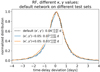 |
Fig. 10. RF evaluated on all samples from its corresponding test set (black dashed line, where training and test sets have the same κ and γ values) and on all samples from two other test sets (blue and orange), with slightly different κ and γ values of the microlensing map in comparison to that of the training data. |
In Fig. 11 we do a similar investigation, but this time we vary the s value of the microlensing maps. From the comparison of the black dashed line to the orange line, which represents almost the same s value, we see that the uncertainties are almost comparable. Therefore, the much wider uncertainty for s = 0.3 (blue line) is not due to variations from different microlensing maps for the same parameter set, but from the fact that lower s values provide more micro caustics in the map, which leads to more events where these caustics are crossed and therefore to more microlensing events and higher uncertainties. This also explains the much tighter uncertainties of s = 0.9, which corresponds to a much smoother microlensing map. These results are in good agreement with those of Huber et al. (2021), who also showed that higher s values lead to lower microlensing uncertainties.
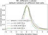 |
Fig. 11. RF evaluated on all samples from its corresponding test set (black dashed line, where training and test sets have the same s value) and on all samples from three other test sets (blue, orange, and green), with different s values of the microlensing map in comparison to that of the training data. |
For a real observation, the s value is often not known very precisely, which is no problem as the RF still works very well. The only thing one has to be careful about is that an underestimation of the s value leads to an overestimation of the overall uncertainties. Therefore, going for a slightly lower s value as one might expect is a good way to obtain a conservative estimate of the uncertainties.
6.2. Uncertainties due to microlensing and noise
In this section we compare the RF from Sect. 5.1 to other RF models with various assumptions about microlensing and noise as shown in Fig. 12.
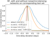 |
Fig. 12. Comparison of the RF model from Sect. 5.1 to three other RF models with hypothetical assumptions about noise and microlensing. Each histogram is based on the whole sample of light curves from their corresponding test set. For our realistic mock observation, the noise in the light curves dominates over microlensing as the main source of uncertainty for measuring the time delays. |
From the two cases containing microlensing in comparison to the two cases without microlensing, we find that microlensing increases the uncertainties almost by a factor of two. Although this is quite substantial, we see that the contribution of the observational noise is much higher and is the dominant source of uncertainty in the time-delay measurement. Therefore, to achieve lower uncertainties, deeper observations with smaller photometric uncertainties are required. This is in agreement with Huber et al. (2019), who found that a substantial increase in the number of LSNe Ia with well measured time delays can be achieved with greater imaging depth.
6.3. Filters used for training
In this section we investigate eight different filters (ugrizyJH) and possible combinations of them to get more precise measurements. Figure 13 shows eight RF models where each is trained and evaluated on a single band. The i band, presented first in Sect. 5.1 provides the most precise measurement. The next promising filters are r, z, g, and y in that order. For the bands u, J, and H, the precision of the measurement is poor and therefore almost not usable. The reason for the strong variation between different bands is the quality of the light curve, which becomes clear from Fig. B.1, where only the g to y bands provide observations where the peak of the light curves can be identified. Light curves with the best quality are the r and i bands, which therefore work best for our RF.
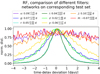 |
Fig. 13. Eight different RF models, each trained on a data set from a single band (as indicated in the legend) and evaluated on the whole sample from the corresponding test set, similar in procedure to Sect. 5.1. |
There are different ways to combine multiple filters to measure the time delay. The first possibility would be to construct color curves to reduce the effect of microlensing in the so-called achromatic phase (Goldstein et al. 2018; Huber et al. 2021). However, as pointed out by Huber et al. (2021) our best quality color curve r − i would be not ideal as there are no features for a delay measurement within the achromatic phase. Further, we saw in Sect. 6.2 that our dominant source of uncertainty is the observational noise instead of microlensing. Therefore, using color curves for this mock example is not practical. We further see that even though color curves are in theory a good way to reduce microlensing uncertainties, in a real detection it might fail because not enough bands with high quality data are available.
Another way of combining multiple filters is to train a single RF model for multiple filters. Generalizing Eq. (4) for the r and i bands, we used as input structure
 (9)
(9)
and more bands will be attached in the same way. The results are summarized in Fig. 14, where we see that combining the two most promising bands improves the uncertainty by about 0.1 days, but adding more bands does not help. Comparing these results to Fig. 15, where different distributions from Fig. 13 are multiplied with each other12, we see that a single RF model for multiple filters does not profit much from multiple bands. Therefore, it is preferable to use a single RF model per band and combine them afterward. Using three or more filters can also help to identify potential biases in a single band as pointed out in Sect. 5.2. Combining the r, i, and z bands via multiplication helps to reduce the uncertainty by more than a factor of two in comparison to using just the i band for our system with zs = 0.76. Further bands that might be considered for follow-up observations are the g and y bands.
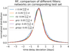 |
Fig. 14. Multiple filters used to train a single RF following the data structure as defined in Eq. (9) (example for ri). Each histogram is based on the whole sample of light curves from their corresponding test set. Using more than two filters does not improve the results further. |
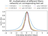 |
Fig. 15. Single RF trained per filter using a similar data structure as in Eq. (4) (example for the i band), leading to six RF models for the six filters g, r, i, z, y, and J. The combination of the filters is done by multiplying the corresponding distributions shown in Fig. 13. We see that multiple filters help to drastically reduce the uncertainties. Therefore, observing three to four bands would be ideal. |
The choice of the ideal filters depends on the source redshift and therefore we show in Fig. G.1 a similar plot as in Fig. 13 but for zs = 0.55 and zs = 0.99, which corresponds to the 16th and 84th percentile of the source redshift from LSNe Ia in the OM10 catalog. From this we learn that the three most promising filters are the g, r, and i bands for zs ≲ 0.6, whereas for zs ≳ 0.6 the r, i, and z bands are preferred. The main reason for this behavior is the low rest-frame UV flux of SNe Ia due to line blanketing, which gets shifted more and more into the g band for higher zs. If four filters could be used, then we have g, r, i, and z for zs ≲ 0.8 and r, i, z, and y for zs ≳ 0.8. If resources for five filters are available, we recommend g, r, i, z, and y; the J band might be preferred over the g band for high source redshifts (zs > 1.0). However, given the poor precision in the g and J bands at such high redshifts, it is questionable how useful the fifth band is in these cases.
7. Machine learning on further mock observations
In this section we investigate further mock systems. We test systems with different moon phases (Sect. 7.1) and source, respectively lens redshifts (Sect. 7.2) to investigate the change of the uncertainties in comparison to our mock system from Sects. 3, 5, and 6. Furthermore, we test the number of data points required before peak to achieve good time-delay measurements (Sect. 7.3) and a quad system with various different properties in comparison to our previous studies (Sect. 7.4).
7.1. Different moon phases
In this section we address the effect of different moon phases. We assume the same LSN Ia as in Sects. 3, 5, and 6, but place it differently in time. From Fig. B.1, we can already estimate that if we ignore the u band, which has too low signal-to-noise anyway, mostly the g band will be influenced as other bands are significantly brighter than the 5σ point-source depth or there is only a minor dependence on the moon phase.
For the LSN Ia presented in Sects. 3, 5, and 6, we see from Fig. B.1 that for the g band, the observations before the peak are significantly affected by moon light, which according to Fig. 13 leads to an uncertainty around 2.1 d. For a case where the peak in the g band overlaps with the full moon we find a similar uncertainty, whereas a case where the peak in the g band matches the new moon has an uncertainty around 1.7 d. For cases where the peak is not significantly brighter than the 5σ point-source depth, the moon phase is important, but given that our ML models work with a variable 5σ point-source depth, the effect of the moon phase is taken into account in our uncertainties. In terms of follow-up observations, one might consider to observe longer at full moon especially in the bluer bands to reach a greater depth or resort to redder bands if the moon will likely affect the observations in the bluer bands adversely, but apart from that, we recommend in general to follow-up all LSNe Ia independently of the moon phase.
7.2. Source and lens redshifts
The mock system we investigated in Sects. 3 and 5 has zs = 0.76, which roughly corresponds to the median source redshift of the OM10 catalog. Furthermore, we have learned from Sect. 6.2 that the observational noise is the dominant source of uncertainty and we therefore expect a large dependence of the time-delay measurement on zs (assuming a fixed exposure time during observations).
We therefore investigate in this section zs = 0.55 and zs = 0.99, which correspond to the 16th and 84th percentiles, respectively, of the source redshift from LSNe Ia in the OM10 catalog. To probe just the dependence on zs, we leave all other parameters as defined in Table 1. We do not scale the absolute time delay with the source redshift, since this is just a hypothetical experiment to demonstrate how different brightnesses, related to the source redshift, influence the time-delay measurement.
The two cases are shown in Fig. 16, where we see the much better quality of the light curve for zs = 0.55 (upper panel) in comparison to zs = 0.99 (lower panel). Further, we also probe the lens redshift by investigating zd = 0.16 and zd = 0.48, which also corresponds to the 16th and 84th percentile of the OM10 catalog and where we also leave other parameters unchanged.
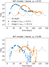 |
Fig. 16. Two LSNe Ia similar to Fig. 3 but with different source redshifts. The LSN Ia in the upper panel has zs = 0.55, and the one in the lower panel has zs = 0.99. |
The results are summarized in Table 5. We see that in comparison to zs = 0.76, the case with zs = 0.55 has an improved uncertainty by ∼0.2 d, where the case zs = 0.99 has a reduced uncertainty by ∼0.7 d. This trend is expected, and means that especially for the case of zs = 0.99, a greater depth would improve the results significantly. Comparing the results of varying lens redshifts, we see a much smaller impact on the uncertainty. Still there is a slight trend that higher lens redshifts correspond to larger time-delay uncertainties, which is in good agreement with Huber et al. (2021), who find the tendency that microlensing uncertainties increase with higher lens redshift if everything else is fixed. The reason for this is that the physical size of the microlensing map decreases with higher lens redshift, which makes a SN Ia appear larger in the microlensing map and therefore events where micro caustics are crossed are more likely. More details are available in Huber et al. (2021).
Time-delay measurement of different LSNe Ia with varying source and lens redshifts.
The impact of the source redshift on the best filters to target is discussed previously in Sect. 6.3.
7.3. Data points before peak
In this section we discuss the number of data points required before peak to achieve a good time-delay measurement. The case presented in Sect. 3 has a large number of data points before peak, which is not always achievable in practice, especially since vetting of transient candidates and triggering of light-curve observations often require additional time. Therefore, we investigate a similar mock system as in Fig. 3, but with a later detection in the first-appearing SN image. In Fig. 17, we show a case where we have the first data point at the peak in the i band in comparison to three other cases where we have four, three, or two data points before the peak. The case for the at-peak detection provides as expected the worst precision but more worrying is the large bias of 0.83 days. Already two data points before peak improve the results significantly and allow precision cosmology for LSNe Ia with a time delay greater than 22 days. Nevertheless, we aim for four data points before peak as we could achieve a bias below 1% already for a delay greater than 10 days; furthermore, the precision is also improved substantially and almost at the level of the mock observation in Fig. 3 and corresponding results in Fig. 8. This would correspond in the observer frame to a detection about eight to ten days before the peak in the i band. Given that a SN Ia typically peaks ∼18 rest-frame days after explosion and the typical lensed SN redshift is ∼0.7, we would need to detect and start follow-up observations of the first-appearing SN image within ∼15 days (observer frame) in order to measure accurate time delays. The results presented here are in good agreement with the feature importance investigations shown in Fig. F.1, where we find that especially the rise slightly before the peak is very important for the RF.
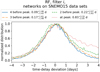 |
Fig. 17. Time-delay deviations of mock observations similar to Fig. 3 but with a later detection, meaning fewer data points before the peak in the i band of the first-appearing SN image. Each histogram is based on the whole sample of light curves from the related SNEMO15 data set. We compare the cases where we have four, three, or two data points before the peak in comparison to an at-peak detection. |
7.4. Quad LSNe Ia and higher microlensing uncertainties
So far we have only discussed double LSNe Ia, but in this section we present a LSN Ia with four images. Our mock quad LSN Ia is similar to the one presented in Sect. 3, but we varied the source position for the double system in the same lensing environment using the GLEE software (Suyu & Halkola 2010; Suyu et al. 2012) such that we get a quad system, where the parameters are listed in Table 6 and the light curves from the system are shown in Fig. 18. For images one to three, the κ and γ values are closer to 0.5 in comparison to the double system from Table 1, which means that the macro magnification is higher but microlensing uncertainties are increased as shown in Huber et al. (2021). For image four, we have κ and γ values far from 0.5; this leads to lower microlensing uncertainties but therefore also to a much fainter image, which can be seen in Fig. 18.
Source redshift, zs, lens redshift, zd, convergence, κ, shear, γ, and the time values for the four images of a mock quad LSN Ia.
In principle such a quad system can be investigated in two ways. The first approach is to train a separate RF per pair of images, leading to six RF models in total. The other way is to train a single RF for the whole quad system that takes as input magnitude values of four images instead of two images, similar to Eq. (4). The outputs as shown in Figs. 5 and 6 are then four instead of two time values.
The results for both approaches are summarized in Table 7 and the correlation plots are shown in Appendix H. We find fewer correlations for the approach “separate RF per pair of images” than for the approach “single RF for all images”, especially for the cases where the noisy fourth image is included in the time-delay measurement. This is because in the first case, six RF models are trained independently from each other, whereas the second case only uses a single RF that predicts four time values for the four images. Still the case “separate RF per pair of images” is preferred because it provides lower biases and tighter constraints. This is not surprising, as providing all the data from the four images at once is a much more complex problem to handle in comparison to training a RF for just two images. While the time-delay deviations between both approaches are almost comparable for pairs of images among the first, second and third images, for the cases where the fourth image is included, the single RF for the whole quad system performs much worse. This suggests that especially handling noisy data can be treated better in the approach of a separate RF for each pair of images and therefore it is always preferred to train a separate RF per pair of images.
In the following we analyze the different uncertainties of the time-delay measurements from different pairs of images as shown in Table 7. The most precise time delay is the one between the first and second image, but if we compare this uncertainty to the uncertainty of the lower panel of Fig. 8 for the double LSNe Ia from Fig. 3, we see that the precision is 0.2 days worse. This can be easily explained by the higher microlensing uncertainties coming from the κ, and γ values much closer to 0.5 as shown in Table 6 in comparison to Table 1. Higher microlensing uncertainties are also the reason why uncertainties of Δt31 and Δt32 are larger than Δt21, even though the third image is the brightest one and therefore has the lowest amount of observational noise. The precision and also accuracy of the time-delay measurement where image four is involved are the worst in Table 7, which is explained by the very poor quality of the light curve from the fourth image. We further see that Δt31 and Δt32 as well as Δt41 and Δt42 have very similar uncertainties, which is expected since light curves from image one and two are almost identical and therefore this is a good check of consistency.
Even though the time-delay measurements between the first three images have the lowest time-delay deviation in days, the absolute time delay is very short, which leads to a very high relative deviation. For this specific mock quad LSNe Ia, it would only make sense to measure time delays with respect to the fourth image, where we would achieve a precision around 10% and an accuracy of 0.7%.
8. Discussion
We train a FCNN with two hidden layers and a RF using four theoretical SN Ia models, to measure time delays in LSNe Ia. We find that both ML models work very well on a test set based on the same four theoretical models used in the training process, providing uncertainties around 0.7 to 0.9 days for the i band almost without any bias. Applying the trained ML models to the SNEMO15 data set, which is composed of empirical SN Ia light curves not used in the training process, we find that the uncertainties increase by about 0.5 days, but this is not surprising as such light curves have never been used in the training process and a measurement with a 1.5-day uncertainty on a single band is still a very good measurement.
However, when applied to the SNEMO15 data set, the FCNN yields biased results. The biases are mostly within 0.4 days, but larger ones are also possible, making our FCNN approach not suitable for precision cosmology. Furthermore, this shows that the generalizability to light-curve shapes not used in the training process is not working for our FCNN approach, since biases on the corresponding test set composed of four theoretical models as used in the training process are negligible. This was already suggested by results presented in Fig. C.1, where the training on three theoretical models was not general enough to perform well on the fourth model not used in the training process. However, we introduced random shifts in time of the light curves, which reduced the bias significantly and motivated us to apply our FCNN trained on four theoretical models (with random shifts in time to reduce the bias), to the SNEMO15 data set as a final test, where we find unfortunately significant biases. Deeper and larger fully connected networks will not solve this problem as they will just fit the training data better and do not guarantee the generalizability. To overcome this, regularization, dropout or uncertainty estimates as additional output to the time values might help. However, this would be some kind of fine tuning to our SNEMO15 data set, because our investigations up to that stage (which shows that our FCNN, trained using three theoretical models, generalizes well to a test set composed of four theoretical models, with negligible resulting biases), were very encouraging to apply our FCNN to the final test (SNEMO15 data set), which it failed. However, we defer further investigations of FCNN to future work, especially since more complex ML approaches such as recurrent neural networks or long short-term memory networks (Sherstinsky 2020) might fit the problem even better.
The RF provides significantly lower biases on the SNEMO15 data set – with 4 or more data points before peak, which means a detection of the first LSNe Ia image about eight to ten days before peak, the bias can be kept within 0.10 days. If one of the images is very faint as shown in Fig. 18, we still can reach an accuracy of 0.15 days and therefore a delay longer than 15 days provides already a time-delay measurement better than 1%. Given the low bias in the RF especially in comparison to the FCNN, the RF is the one to use for a real application.
Huber et al. (2019) used the free-knot spline estimator from PyCS (Tewes et al. 2013; Bonvin et al. 2016) to measure time delays for LSNe Ia. To compare this approach to our results, we apply PyCS as used in Huber et al. (2019) to the SNEMO15 data set. For the system shown in Fig. 3 with a very well sampled light curve, we achieve similar uncertainties as the RF shown in Fig. 8. However, as soon as we look at cases, where we have a reduced number of data points before peak as shown in Fig. 19 (in comparison to the RF results in Fig. 17), we see that the RF approach achieves a much higher precision. In terms of the bias, as long as we provide two data points or more before peak the RF and PyCS provide sufficient results. For the case where the first data point is at the peak of the i band, even though PyCS provides a much better bias than the RF, the measurement has substantially poorer precision. Overall the RF works better to measure time delays in LSNe Ia in most cases in comparison to PyCS. However in a real application, both approaches could be used to cross-check the time-delay measurements.
9. Summary
In this work we have introduced two ML techniques, namely a deep learning network using a FCNN with two hidden layers and a RF to measure time delays of LSNe Ia. We simulated LSN Ia light curves for the training process, including observational noise and microlensing uncertainties using four different theoretical models. Our training set is composed of 400 000 LSNe Ia coming from 4 theoretical models, 10 000 microlensing map positions, and 10 noise realizations. Our test set has a size of 40 000 LSNe Ia, and we drew 1000 microlensing map positions instead of 10 000 as for the training set. We constructed a further data set based on the empirical SNEMO15 model to create realistic LSN Ia light curves not used in the training process to check if our approach is general enough to handle real observations of LSNe Ia. To add microlensing to the SNEMO15 model, we used the microlensed light curves from the theoretical models, subtracting the macrolensed light curve to get the microlensing contribution.
To summarize our results, we looked at the more realistic results from the empirical SNEMO15 data set. From the investigation of the RF and the FCNN, we find that only the RF provides sufficiently low bias and is therefore the approach to use in a real application. From all investigated systems where we assumed a two-day cadence with a few random gaps, we found that we can achieve an accuracy better than 1% for the RF if we restrict ourselves to LSN Ia systems with a delay longer than 15 days, where we obtain the first data point around eight to ten days before the peak in the light curve of the first-appearing SN image. In terms of precision, we can achieve an uncertainty of 1.5 days from the i band alone for the median source redshift ∼0.76 of LSNe Ia in OM10. Using three bands where the time delay is measured separately for each RF and combined afterward, we can reach an approximately 1.0-day uncertainty. The three most promising filters to target are g, r, and i for zs ≲ 0.6 and r, i, and z for higher source redshifts. As a fourth and fifth band, the z and y for zs ≲ 0.6 and the g and y for zs ≳ 0.6 might be considered. We find that the gain from multiple filters is the best if a ML model is trained individually per band. The other bands investigated in this work (u, J, and H) provide very poor-quality light curves and are therefore not useful.
From our investigations, we find mainly that the observational noise is the dominant source of uncertainty in measuring time delays, and to improve the results presented here, a greater depth would be required. The depth we assumed for follow-up observations is one magnitude deeper than the single-epoch LSST-like 5σ depth, meaning 25.7, 25.3, 24.7, 23.8, and 23.0 for g, r, i, z, and y, respectively. From the investigation of the source redshifts, we find that in comparison to the median source redshift of ∼0.76 of LSNe Ia in OM10, zs = 0.55 can improve the precision in the i band by 0.2 days, but zs = 0.99 might lower the uncertainty by 0.7 days, which suggests that, especially for higher source redshifts, a greater depth might be required. Although a greater depth could also compensate for the moon phase, the impact on the uncertainty is weaker (an at most 0.4 days worse uncertainty in our investigation) and becomes even less relevant the redder the bands are. We further find that typical uncertainties in the microlensing parameters (κ, γ, and s) are not relevant for our training process. Only a significantly overestimated s value would lead to an underestimation of the uncertainties. Furthermore, we find that our approach works best if an individual RF is trained per pair of images.
In comparison to the free-knot spline estimator from PyCS (Tewes et al. 2013; Bonvin et al. 2016) as used in Huber et al. (2019), our approach works better overall, providing an improved precision of up to ∼0.8 days. We therefore can expect slightly more LSNe Ia with well-measured time delays than the number predicted by Huber et al. (2019).
In this work we have developed a new method to measure time delays of LSNe Ia. The RF provides accurate and precise time-delay measurements that are comparable with or better than current methods and is therefore an important tool to pave the way for LSNe Ia as cosmological probes. The downsides of our approach are: that a RF needs to be trained separately for each individual system’s observing pattern; the dependence on the SN Ia models used in the training process; and that our approach cannot for the moment be applied to other types of LSNe. A highly promising approach to overcoming this and building a ML network that is more general is the use of recurrent neural networks or long short-term memory networks (Sherstinsky 2020), which will be investigated in a future study.
Of the fainter image for a double system; for a quad system, the peak brightness of the third brightest image is considered.
To avoid unrealistically noisy data points, we limit the maximum amount of noise allowed, as described in Appendix A.
For the other hyperparameters of the Adam optimizer, we used the PyTorch default values.
A single feature such as mi1, 2 can be picked multiple times.
Further splitting is not useful if none of the investigated splitting criteria would lead to further improvements of the sum of squared residuals in comparison to not splitting the remaining samples.
Such hyperparameter optimizations are usually performed using the validation set, whereas we are using the test set because we have the SNEMO15 data set for ultimate performance test.
Inductive bias refers to the bias coming from assumptions that a ML model has to make to generalize based on training samples.
We assume that different filters have independent detector noise.
Acknowledgments
We thank F. Courbin, S. Schuldt and R. Cañameras for useful discussions. We also would like to thank the anonymous referee for helpful feedback, which strengthened this work. SH and SHS thank the Max Planck Society for support through the Max Planck Research Group for SHS. This project has received funding from the European Research Council (ERC) under the European Union’s Horizon 2020 research and innovation programme (grant agreement No 771776). This research is supported in part by the Excellence Cluster ORIGINS which is funded by the Deutsche Forschungsgemeinschaft (DFG, German Research Foundation) under Germany’s Excellence Strategy – EXC-2094 – 390783311. DG acknowledges support from the Baden-Württemberg Foundation through the Baden-Württemberg Eliteprogramm for Postdocs. UMN has been supported by the Transregional Collaborative Research Center TRR33 “The Dark Universe” of the Deutsche Forschungsgemeinschaft. JHHC acknowledges support from the Swiss National Science Foundation and through European Research Council (ERC) under the European Union’s Horizon 2020 research and innovation programme (COSMICLENS: grant agreement No 787866). MK acknowledges support from the Klaus Tschira Foundation.
References
- Abbott, B. P., Abbott, R., Abbott, T. D., et al. 2017, Nature, 551, 85 [Google Scholar]
- Anand, G. S., Tully, R. B., Rizzi, L., Riess, A. G., & Yuan, W. 2021, AAS J., submitted [arXiv:2108.00007] [Google Scholar]
- Barnabè, M., Czoske, O., Koopmans, L. V. E., Treu, T., & Bolton, A. S. 2011, MNRAS, 415, 2215 [Google Scholar]
- Bessell, M., & Murphy, S. 2012, PASP, 124, 140 [NASA ADS] [CrossRef] [Google Scholar]
- Birrer, S., Treu, T., Rusu, C. E., et al. 2019, MNRAS, 484, 4726 [Google Scholar]
- Birrer, S., Shajib, A. J., Galan, A., et al. 2020, A&A, 643, A165 [NASA ADS] [CrossRef] [EDP Sciences] [Google Scholar]
- Blakeslee, J. P., Jensen, J. B., Ma, C.-P., Milne, P. A., & Greene, J. E. 2021, ApJ, 911, 65 [NASA ADS] [CrossRef] [Google Scholar]
- Bonvin, V., & Millon, M. 2020, https://doi.org/10.5281/zenodo.3635517 [Google Scholar]
- Bonvin, V., Tewes, M., Courbin, F., et al. 2016, A&A, 585, A88 [NASA ADS] [CrossRef] [EDP Sciences] [Google Scholar]
- Bonvin, V., Chan, J. H. H., Millon, M., et al. 2018, A&A, 616, A183 [NASA ADS] [CrossRef] [EDP Sciences] [Google Scholar]
- Breiman, L. 2001, Mach. Learn., 45, 5 [Google Scholar]
- Buitinck, L., Louppe, G., Blondel, M., et al. 2013, ECML PKDD Workshop: Languages for Data Mining and Machine Learning, 108 [Google Scholar]
- Chan, J. H. H., Rojas, K., Millon, M., et al. 2021, A&A, 647, A115 [NASA ADS] [CrossRef] [EDP Sciences] [Google Scholar]
- Chang, K., & Refsdal, S. 1979, Nature, 282, 561 [Google Scholar]
- Chen, G. C.-F., Fassnacht, C. D., Suyu, S. H., et al. 2019, MNRAS, 490, 1743 [NASA ADS] [CrossRef] [Google Scholar]
- Courbin, F., Bonvin, V., Buckley-Geer, E., et al. 2018, A&A, 609, A71 [NASA ADS] [CrossRef] [EDP Sciences] [Google Scholar]
- Cybenko, G. 1989, Math. Control Signals Syst., 2, 303 [Google Scholar]
- Ding, X., Liao, K., Birrer, S., et al. 2021, MNRAS, 504, 5621 [NASA ADS] [CrossRef] [Google Scholar]
- Falco, E. E., Gorenstein, M. V., & Shapiro, I. I. 1985, ApJ, 289, L1 [Google Scholar]
- Foreman-Mackey, D. 2016, J. Open Sour. Softw., 1, 24 [NASA ADS] [CrossRef] [Google Scholar]
- Foxley-Marrable, M., Collett, T. E., Vernardos, G., Goldstein, D. A., & Bacon, D. 2018, MNRAS, 478, 5081 [NASA ADS] [CrossRef] [Google Scholar]
- Freedman, W. L., Madore, B. F., Hatt, D., et al. 2019, ApJ, 882, 34 [Google Scholar]
- Freedman, W. L., Madore, B. F., Hoyt, T., et al. 2020, ApJ, 891, 57 [Google Scholar]
- Glorot, X., Bordes, A., & Bengio, Y. 2010, J. Mach. Learn. Res., 15, 315 [Google Scholar]
- Goldstein, D. A., & Nugent, P. E. 2017, ApJ, 834, L5 [Google Scholar]
- Goldstein, D. A., Nugent, P. E., Kasen, D. N., & Collett, T. E. 2018, ApJ, 855, 22 [NASA ADS] [CrossRef] [Google Scholar]
- Goobar, A., Amanullah, R., Kulkarni, S. R., et al. 2017, Science, 356, 291 [Google Scholar]
- Hornik, K., Stinchcombe, M., & White, H. 1989, Neural Netw., 2, 359 [NASA ADS] [CrossRef] [Google Scholar]
- Huber, S., Suyu, S. H., Noebauer, U. M., et al. 2019, A&A, 631, A161 [NASA ADS] [CrossRef] [EDP Sciences] [Google Scholar]
- Huber, S., Suyu, S. H., Noebauer, U. M., et al. 2021, A&A, 646, A110 [NASA ADS] [CrossRef] [EDP Sciences] [Google Scholar]
- Irwin, M. J., Webster, R. L., Hewett, P. C., Corrigan, R. T., & Jedrzejewski, R. I. 1989, AJ, 98, 1989 [NASA ADS] [CrossRef] [Google Scholar]
- Ivezic, Ž., Kahn, S. M., Tyson, J. A., et al. 2019, ApJ, 873, 111 [NASA ADS] [CrossRef] [Google Scholar]
- Kasen, D., Thomas, R. C., & Nugent, P. 2006, ApJ, 651, 366 [NASA ADS] [CrossRef] [Google Scholar]
- Kelly, P. L., Rodney, S. A., Treu, T., et al. 2016a, ApJ, 819, L8 [NASA ADS] [CrossRef] [Google Scholar]
- Kelly, P. L., Brammer, G., Selsing, J., et al. 2016b, ApJ, 831, 205 [NASA ADS] [CrossRef] [Google Scholar]
- Khetan, N., Izzo, L., Branchesi, M., et al. 2021, A&A, 647, A72 [NASA ADS] [CrossRef] [EDP Sciences] [Google Scholar]
- Kingma, D. P., & Ba, J. 2014, ArXiv e-prints [arXiv:1412.6980] [Google Scholar]
- Kochanek, C. S. 2020, MNRAS, 493, 1725 [NASA ADS] [CrossRef] [Google Scholar]
- Krishnan, C., Mohayaee, R., Colgáin, E. Ó., Sheikh-Jabbari, M. M., & Yin, L. 2021a, Classical Quantum Gravity, 38, 184001 [NASA ADS] [CrossRef] [Google Scholar]
- Krishnan, C., Mohayaee, R., Colgáin, E., Sheikh-Jabbari, M. M., & Yin, L. 2021b, ArXiv e-prints [arXiv:2106.02532] [Google Scholar]
- Kromer, M., & Sim, S. A. 2009, MNRAS, 398, 1809 [Google Scholar]
- LSST Science Collaboration (Abell, P. A., et al.) 2009, ArXiv e-prints [arXiv:0912.0201] [Google Scholar]
- Maas, A. L., Hannun, A. Y., & Ng, A. Y. 2013, ICML Workshop on Deep Learning for Audio, Speech and Language Processing [Google Scholar]
- Mediavilla, E., Muñoz, J. A., Garzón, F., & Mahoney, T. J. 2016, Astrophysical Applications of Gravitational Lensing (Cambridge: Cambridge University Press) [CrossRef] [Google Scholar]
- Millon, M., Galan, A., Courbin, F., et al. 2020, A&A, 639, A101 [NASA ADS] [CrossRef] [EDP Sciences] [Google Scholar]
- More, A., Suyu, S. H., Oguri, M., More, S., & Lee, C.-H. 2017, ApJ, 835, L25 [Google Scholar]
- Nomoto, K., Thielemann, F.-K., & Yokoi, K. 1984, ApJ, 286, 644 [NASA ADS] [CrossRef] [Google Scholar]
- Oguri, M., & Kawano, Y. 2003, MNRAS, 338, L25 [NASA ADS] [CrossRef] [Google Scholar]
- Oguri, M., & Marshall, P. J. 2010, MNRAS, 405, 2579 [NASA ADS] [Google Scholar]
- Pakmor, R., Kromer, M., Taubenberger, S., et al. 2012, ApJ, 747, L10 [NASA ADS] [CrossRef] [Google Scholar]
- Paszke, A., Gross, S., Massa, F., et al. 2019, in Advances in Neural Information Processing Systems 32, eds. H. Wallach, H. Larochelle, A. Beygelzimer, et al. (Curran Associates, Inc.), 8024 [Google Scholar]
- Pedregosa, F., Varoquaux, G., Gramfort, A., et al. 2011, J. Mach. Learn. Res., 12, 2825 [Google Scholar]
- Pesce, D. W., Braatz, J. A., Reid, M. J., et al. 2020, ApJ, 891, L1 [Google Scholar]
- Pierel, J. D. R., & Rodney, S. 2019, ApJ, 876, 107 [NASA ADS] [CrossRef] [Google Scholar]
- Planck Collaboration I. 2020, A&A, 641, A1 [NASA ADS] [CrossRef] [EDP Sciences] [Google Scholar]
- Quimby, R. M., Oguri, M., More, A., et al. 2014, Science, 344, 396 [NASA ADS] [CrossRef] [Google Scholar]
- Refsdal, S. 1964, MNRAS, 128, 307 [NASA ADS] [CrossRef] [Google Scholar]
- Riess, A. G., Macri, L. M., Hoffmann, S. L., et al. 2016, ApJ, 826, 56 [Google Scholar]
- Riess, A. G., Casertano, S., Yuan, W., et al. 2018, ApJ, 861, 126 [NASA ADS] [CrossRef] [Google Scholar]
- Riess, A. G., Casertano, S., Yuan, W., Macri, L. M., & Scolnic, D. 2019, ApJ, 876, 85 [Google Scholar]
- Riess, A. G., Casertano, S., Yuan, W., et al. 2021, ApJ, 908, L6 [NASA ADS] [CrossRef] [Google Scholar]
- Rodney, S. A., Brammer, G. B., Pierel, J. D. R., et al. 2021, Nat. Astron., 5, 1118 [NASA ADS] [CrossRef] [Google Scholar]
- Rusu, C. E., Wong, K. C., Bonvin, V., et al. 2020, MNRAS, 498, 1440 [Google Scholar]
- Saunders, C., Aldering, G., Antilogus, P., et al. 2018, ApJ, 869, 167 [NASA ADS] [CrossRef] [Google Scholar]
- Schneider, P., & Sluse, D. 2013, A&A, 559, A37 [NASA ADS] [CrossRef] [EDP Sciences] [Google Scholar]
- Schneider, P., & Sluse, D. 2014, A&A, 564, A103 [NASA ADS] [CrossRef] [EDP Sciences] [Google Scholar]
- Seitenzahl, I. R., Ciaraldi-Schoolmann, F., Röpke, F. K., et al. 2013, MNRAS, 429, 1156 [NASA ADS] [CrossRef] [Google Scholar]
- Shajib, A. J., Treu, T., & Agnello, A. 2018, MNRAS, 473, 210 [Google Scholar]
- Shajib, A., Birrer, S., Treu, T., et al. 2020, MNRAS, 494, 6072 [NASA ADS] [CrossRef] [Google Scholar]
- Sherstinsky, A. 2020, Phys. D: Nonlinear Phenom., 404, 132306 [NASA ADS] [CrossRef] [Google Scholar]
- Sim, S. A., Röpke, F. K., Hillebrandt, W., et al. 2010, ApJ, 714, L52 [Google Scholar]
- Sluse, D., Rusu, C. E., Fassnacht, C. D., et al. 2019, MNRAS, 490, 613 [NASA ADS] [CrossRef] [Google Scholar]
- Suyu, S. H., & Halkola, A. 2010, A&A, 524, A94 [NASA ADS] [CrossRef] [EDP Sciences] [Google Scholar]
- Suyu, S. H., Hensel, S. W., McKean, J. P., et al. 2012, ApJ, 750, 10 [Google Scholar]
- Suyu, S. H., Bonvin, V., Courbin, F., et al. 2017, MNRAS, 468, 2590 [Google Scholar]
- Suyu, S. H., Huber, S., Cañameras, R., et al. 2020, A&A, 644, A162 [NASA ADS] [CrossRef] [EDP Sciences] [Google Scholar]
- Tewes, M., Courbin, F., & Meylan, G. 2013, A&A, 553, A120 [NASA ADS] [CrossRef] [EDP Sciences] [Google Scholar]
- Verde, L., Treu, T., & Riess, A. G. 2019, Nat. Astron., 3, 891 [Google Scholar]
- Vernardos, G., & Fluke, C. J. 2014, Astron. Comput., 6, 1 [Google Scholar]
- Vernardos, G., Fluke, C. J., Bate, N. F., & Croton, D. 2014, ApJS, 211, 16 [NASA ADS] [CrossRef] [Google Scholar]
- Vernardos, G., Fluke, C. J., Bate, N. F., Croton, D., & Vohl, D. 2015, ApJS, 217, 23 [CrossRef] [Google Scholar]
- Wambsganss, J. 2006, 33rd Advanced Saas Fee Course on Gravitational Lensing: Strong, Weak, and Micro, 453 [NASA ADS] [CrossRef] [Google Scholar]
- Wilson, A. G., & Izmailov, P. 2020, ArXiv e-prints [arXiv:2002.08791] [Google Scholar]
- Wojtak, R., Hjorth, J., & Gall, C. 2019, MNRAS, 487, 3342 [Google Scholar]
- Wong, K. C., Suyu, S. H., Chen, G. C. F., et al. 2020, MNRAS, 498, 1420 [Google Scholar]
- Yahalomi, D. A., Schechter, P. L., & Wambsganss, J. 2017, ArXiv e-prints [arXiv:1711.07919] [Google Scholar]
- Yıldırım, A., van den Bosch, R. C. E., van de Ven, G., et al. 2017, MNRAS, 468, 4216 [Google Scholar]
- Yıldırım, A., Suyu, S. H., & Halkola, A. 2020, MNRAS, 493, 4783 [Google Scholar]
Appendix A: Photometric uncertainties
The photometric uncertainty σ1 from Eq. 3 is defined as:
 (A.1)
(A.1)
and
 (A.2)
(A.2)
The parameter γc varies from 0.037 to 0.040 for different filters and x = 100.4(mAB, X − m5), where mAB, X is the AB magnitude in filter X from Eq. (2) of the SN data point and m5 is the 5σ point-source depth (for more details, see LSST Science Collaboration 2009, Sect. 3.5, p. 67).
A magnitude value mAB, X, which is much higher (fainter) than the 5σ point-source depth m5, can lead to unrealistic mdata, X in Eq. (3). Normally one would just delete such a data point, but for our ML model this is not possible, given that we always need the same number of data points as input. Therefore, to avoid such outliers in our data set used for training, validation and testing, we ensure that all magnitude values lower than m5 cannot exceed m5 (bright data point just due to large error) or be much fainter than this value (data point not observable). Specifically, if the SN image brightness mAB, X (see Eq. (3)) is fainter than m5 and the calculated uncertainties would lead to a mdata, X that is smaller (brighter) than m5 or larger (fainter) than maxt(mAB, X(t)) + (maxt(mAB, X(t)) − m5), we replace that data point with a uniform random number between m5 and mAB, X + (mAB, X − m5), where the term (mAB, X − m5) ensures that the uniform random number can be fainter than mAB, X, but not by more than the magnitude difference between mAB, X and m5.
Appendix B: Light curves of mock observation in multiple bands
Figure B.1 shows all the bands from the mock observation discussed in Sects. 3, 5, and 6.
 |
Fig. B.1. Further bands for the mock observation of Sect. 3. The dashed gray line marks the 5σ point-source depth that accounts for the moon phase. |
Appendix C: Bias reduction: Training on three models
In this section we discuss some hypothetical cases where we assume that only three of the four theoretical models are available for the training of the ML method.
We start with the FCNN as described in Sect. 4.1 and investigate four different cases namely: (merger, N100, sub-Ch), (merger, N100, W7), (merger, sub-Ch, W7), and (N100, sub-Ch, W7) for the training process. The black solid line in each panel of Fig. C.1 shows the case where the trained model is evaluated on the corresponding test set, meaning that the test set contains light curves from all three models in the same fraction as in the training data. The other four distributions, shown in each panel, correspond to the evaluation of the FCNN trained on 3 models, on a test set that contains just light curves from a single SN Ia model. The shown results are the median (50th percentile), with the 84th–50th percentile (superscript) and 16th–50th percentile (subscript). The left column contains the normalized light curves as displayed in Fig. 1 and the right column contains the same models but during the training process we allow for a random shift in time from [−5, 5] days and a random shift in magnitude from [−0.4, 0.4]. We only apply the shifts in the training set and not in the test set although the results look similar. While the shift in magnitude is only applied to make the noise level more flexible, the shifts in time help to increase the variety of the light curves, especially so that the locations of the peak from different models do overlap.
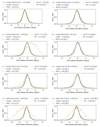 |
Fig. C.1. FCNNs trained on three SN Ia models and evaluated on all samples of its corresponding test set, in comparison to the evaluation on all samples from four test sets from the four individual SN Ia models. The left column shows the case where the SN Ia models have been used as shown in Fig. 1. The right column contains plots in which the SN Ia models are randomly shifted within ±5 d in time and ±0.4 in magnitude. The random shifts make the training set generalize better to test sets that are not represented by the training set. |
From the left column of Fig. C.1, we learn that as soon as a model was included in the training process the network performs very well on the test set of the model. For the case of (merger, N100, sub-Ch) for the training process, the network works also very well on the test set from W7, even though it has never seen light curves from that model. The reason for that seems to be that light curves from the W7 model are close to the sub-Ch model for early times and close to the N100 model in later times (especially for the rest-frame g band) as shown in Fig. 1. The other three cases still work on the model it was not trained on, but we detect biases on the order of almost a day, especially for the sub-Ch and merger model (left column, rows two and four). From the right column of Fig. C.1 we find that our applied random shifts in time and magnitude significantly help to overcome these biases. Even though this broadens the distributions of the models it was trained on slightly, it tightens the distribution of the models it was not trained on and therefore helps to generalize to real observations.
In Fig. C.2 we do the same experiment but this time using the RF. For the cases (merger, N100, sub-Ch), (merger, N100, W7), and (merger, sub-Ch, W7) we find that applying the random shifts in the training process improves the bias and precision on the test set based on the model not used in the training process. Only for the case of using (N100, sub-Ch, W7) in the training process the merger results get worse. This suggests that especially the merger model, which deviates most from the other three models as shown in Fig. 1 and therefore helps to increase the variaty, is required in the training process. However, the comparison between Figs. C.1 and C.2 shows that the RF does already a pretty good job without the random shifts, and therefore the RF generalizes better to slightly different light-curve shapes in comparison to our FCNN approach. Nevertheless, the results from the right column of Fig. C.1 are an encouraging sign that with the random shifts in time our FCNN approach can also be generalized better to SN Ia light curves, which were not used in the training process.
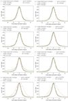 |
Fig. C.2. RF networks trained on three SN Ia models and evaluated on all samples of their corresponding test set, in comparison to the evaluation on all samples from four test sets from the four individual SN Ia models. The left column shows the case where the SN Ia models have been used as shown in Fig. 1. The right column contains plots where the SN Ia models are randomly shifted within ±5 d in time and ±0.4 in magnitude. The random shifts are far less important than for the FCNN approach shown in Fig. C.1. |
Instead of random shifts in time, one might argue that different random multiplication factors that stretch or squeeze the light curves in time might work even better. Therefore, we tested different ranges for the random factors, namely, (0.95 to 1.05), (0.9 to 1.1), (0.85 to 1.15), (0.8 to 1.2), (0.7 to 1.3), (0.6 to 1.4), (0.5 to 1.5), and (0.2 to 1.8), where the factor 1 provides the light curves as shown in Fig. 1. We find that (0.7 to 1.3) works best to reduce biases in a similar way as shown in Fig. C.1. Nevertheless applying a FCNN and RF model trained on four theoretical models with the random multiplication factors to an empirical data set based on SNEMO15 similar as in Sect. 5.2, we find that even though the precision for the FCNN is roughly 0.05 days better as in Fig. 8 the FCNN still predicts substantial biases for the SNEMO15 data set up to 0.5 days and is therefore not useful. Furthermore, the precision of the RF on the SNEMO15 data set for the random shifts in time between [−5, 5] days (as shown in Fig. 8) is roughly 0.2 days better than results from using random multiplication factors and therefore using the random shifts in time was a valuable choice.
Appendix D: Train and validation loss
In Fig. D.1 we see for the FCNN the training loss in comparison to the validation loss for 400 training epochs. The network that provides the lowest validation loss is the one that will be stored to reduce the chance of overfitting the training data.
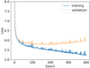 |
Fig. D.1. Training and validation loss of the FCNN for 400 training epochs. |
Appendix E: Time-delay deviation as a function of time delay
Figure E.1 shows the time-delay deviation as a function of time for the LSN Ia from Fig. 4.
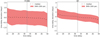 |
Fig. E.1. Time-delay deviation, τi, from Eq. (8) as a function of the time delay, where we have binned up the samples from the corresponding test set with similar time delays (bin size: two days) for the LSN Ia from Fig. 4. The vertical gray line marks the true absolute time delay from the mock LSN Ia system. The corresponding test set has LSN Ia systems that span a range of input time-delay values, which include the vertical gray line. Results from the FCNN network are shown in the left panel, and the RF is presented in the right panel. |
Appendix F: Feature importance of FCNN and RF
In this section we investigate which of the features in Eq. (4) are the most important ones for the FCNN and the RF. For the FCNN the estimate is difficult and therefore we consider as an approximation just the input layer, where we calculate for each feature (input node) the mean of all the weights connected to that feature (negative weights are removed because a ReLU activation function is used). The results are summarized in the upper panel of Fig. F.1, where we see that the FCNN focuses mainly on the region of the peak.
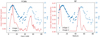 |
Fig. F.1. Evaluation of the features (input nodes) for the FCNN (left panel) and the RF (right panel). The features (input nodes) are listed in Eq. (4), where feature 1 stands for mi1, 1 and the last feature (81) is mi2, Ni2. |
To estimate the importance of the features for the RF we use from the software scikit-learn the feature_importances_tool13 (Pedregosa et al. 2011; Buitinck et al. 2013). This tool basically measures the decrease in performance of a RF if a specific feature would be removed. The results are shown in the lower panel of Fig. F.1. Comparing these results to the FCNN, we find that the RF is mainly focusing on the rise before the peak but also the decline afterward is important. The peak itself does not matter much. We further see that the noisy part of the light curves is almost not considered in comparison to the FCNN. Focusing on higher signal-to-noise data points, less on the peak and more on the rise and decline seems to help the RF to perform better on the empirical SNEMO15 data set in comparison to the FCNN.
Appendix G: Filters for different redshifts
Figure G.1 shows the performance of the RF on different filters for zs = 0.55 and zs = 0.99.
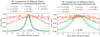 |
Fig. G.1. Both panels show different RF models, each trained on a data set from a single band (as indicated in the legend) and evaluated on all samples from the corresponding test set. The left panel shows the case for zs = 0.55, and the right panel shows zs = 0.99, without the u band, which is already too faint for such a source redshift. |
Appendix H: Correlation plots
Figures H.1 and H.2 show the correlation plots (Foreman-Mackey 2016) for a quad system of a LSN Ia using a separate RF model per pair of images in comparison to a single RF for all images.
 |
Fig. H.1. Correlation plots using separate RF models per pair of images for the LSN Ia quad system shown in Fig. 18. The contour plot shows the 1σ, 2σ, and 3σ contours. The dashed lines in the histograms correspond to the median and the 1σ and 2σ range. |
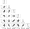 |
Fig. H.2. Correlation plots using a single RF model for all images for the LSN Ia quad system shown in Fig. 18. The contour plot shows the 1σ, 2σ, and 3σ contours. The dashed lines in the histograms correspond to the median and the 1σ and 2σ range. |
All Tables
Mock system of the OM10 catalog for generating mock light curves to train our ML techniques.
Time-delay measurement of different LSNe Ia with varying source and lens redshifts.
Source redshift, zs, lens redshift, zd, convergence, κ, shear, γ, and the time values for the four images of a mock quad LSN Ia.
All Figures
|
Fig. 1. Normalized LSST u- and g-band rest-frame light curves for four theoretical SN Ia models (merger, N100, sub-Ch, and W7) in comparison to the empirical model SNEMO15. |
| In the text | |
|
Fig. 2. Estimated 5σ depth for eight different filters, u, g, r, i, z, y, J, and H, accounting for the moon phase. Day 0 corresponds to the first quarter in the moon phase. Full moon is around day 8, and new moon is on day 23. |
| In the text | |
|
Fig. 3. Simulated observation for which ML models will be trained to measure the time delay. The gray dashed curve marks the 5σ point-source depth, that accounts for the moon phase. The marked data points are also listed in Eq. (4). |
| In the text | |
|
Fig. 4. Simulated data to train a ML model. The filled dots correspond to the mock observation shown in Fig. 3. The open dots represent the simulated training samples, where two out of the 400 000 are shown for the i band in the top and bottom panels. |
| In the text | |
|
Fig. 5. FCNN, where the input layer has Nd data points and dj stands for the magnitude value of the jth data point in Eq. (4). The size of the two hidden layers scales by a factor f, and the outputs are two (four) time values for a double (quad) LSN Ia. |
| In the text | |
|
Fig. 6. Schematic example of a regression tree for a double system that predicts two time values for certain input data as in Eq. (4). The root node is represented by the magenta box, the internal nodes by gray boxes, and the leaf nodes by green boxes. |
| In the text | |
|
Fig. 7. FCNN and RF on the whole sample of light curves from the specified test set for the mock observation in Fig. 3. The ML models’ hyperparameters are set to the values at which the test set yields a bias below 0.05 days and the smallest 68% credible interval of the time-delay deviation (in Eq. (8)). |
| In the text | |
|
Fig. 8. FCNN and RF trained on four theoretical models for the i band evaluated on the whole sample of light curves from the two specified data sets. The dashed black line represents the corresponding test set based on the four theoretical models, and the data set of the blue line is based on the empirical SNEMO15 model. |
| In the text | |
|
Fig. 9. Bias of FCNN and RF on the corresponding test set, composed of four theoretical SN Ia models used for training, and a data set based on the empirical SNEMO15 model, not used during training, for a variety of different hyperparameters and filters (i, z, and y), i.e., from model averaging. The large biases on the SNEMO15 data set up to 1 day in our FCNN approach come from the different hyperparameters even though the corresponding test set provides biases within 0.25 days. The RF provides much lower biases in all cases; it depends only weakly on the hyperparameters and is instead mostly set by the filters under consideration. |
| In the text | |
|
Fig. 10. RF evaluated on all samples from its corresponding test set (black dashed line, where training and test sets have the same κ and γ values) and on all samples from two other test sets (blue and orange), with slightly different κ and γ values of the microlensing map in comparison to that of the training data. |
| In the text | |
|
Fig. 11. RF evaluated on all samples from its corresponding test set (black dashed line, where training and test sets have the same s value) and on all samples from three other test sets (blue, orange, and green), with different s values of the microlensing map in comparison to that of the training data. |
| In the text | |
|
Fig. 12. Comparison of the RF model from Sect. 5.1 to three other RF models with hypothetical assumptions about noise and microlensing. Each histogram is based on the whole sample of light curves from their corresponding test set. For our realistic mock observation, the noise in the light curves dominates over microlensing as the main source of uncertainty for measuring the time delays. |
| In the text | |
|
Fig. 13. Eight different RF models, each trained on a data set from a single band (as indicated in the legend) and evaluated on the whole sample from the corresponding test set, similar in procedure to Sect. 5.1. |
| In the text | |
|
Fig. 14. Multiple filters used to train a single RF following the data structure as defined in Eq. (9) (example for ri). Each histogram is based on the whole sample of light curves from their corresponding test set. Using more than two filters does not improve the results further. |
| In the text | |
|
Fig. 15. Single RF trained per filter using a similar data structure as in Eq. (4) (example for the i band), leading to six RF models for the six filters g, r, i, z, y, and J. The combination of the filters is done by multiplying the corresponding distributions shown in Fig. 13. We see that multiple filters help to drastically reduce the uncertainties. Therefore, observing three to four bands would be ideal. |
| In the text | |
|
Fig. 16. Two LSNe Ia similar to Fig. 3 but with different source redshifts. The LSN Ia in the upper panel has zs = 0.55, and the one in the lower panel has zs = 0.99. |
| In the text | |
|
Fig. 17. Time-delay deviations of mock observations similar to Fig. 3 but with a later detection, meaning fewer data points before the peak in the i band of the first-appearing SN image. Each histogram is based on the whole sample of light curves from the related SNEMO15 data set. We compare the cases where we have four, three, or two data points before the peak in comparison to an at-peak detection. |
| In the text | |
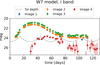 |
Fig. 18. Light curves of the mock quad LSN Ia from Table 6 for the i band. |
| In the text | |
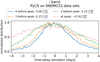 |
Fig. 19. Same as Fig. 17 but this time using PyCS on all samples from the SNEMO15 data set. |
| In the text | |
|
Fig. B.1. Further bands for the mock observation of Sect. 3. The dashed gray line marks the 5σ point-source depth that accounts for the moon phase. |
| In the text | |
|
Fig. C.1. FCNNs trained on three SN Ia models and evaluated on all samples of its corresponding test set, in comparison to the evaluation on all samples from four test sets from the four individual SN Ia models. The left column shows the case where the SN Ia models have been used as shown in Fig. 1. The right column contains plots in which the SN Ia models are randomly shifted within ±5 d in time and ±0.4 in magnitude. The random shifts make the training set generalize better to test sets that are not represented by the training set. |
| In the text | |
|
Fig. C.2. RF networks trained on three SN Ia models and evaluated on all samples of their corresponding test set, in comparison to the evaluation on all samples from four test sets from the four individual SN Ia models. The left column shows the case where the SN Ia models have been used as shown in Fig. 1. The right column contains plots where the SN Ia models are randomly shifted within ±5 d in time and ±0.4 in magnitude. The random shifts are far less important than for the FCNN approach shown in Fig. C.1. |
| In the text | |
|
Fig. D.1. Training and validation loss of the FCNN for 400 training epochs. |
| In the text | |
|
Fig. E.1. Time-delay deviation, τi, from Eq. (8) as a function of the time delay, where we have binned up the samples from the corresponding test set with similar time delays (bin size: two days) for the LSN Ia from Fig. 4. The vertical gray line marks the true absolute time delay from the mock LSN Ia system. The corresponding test set has LSN Ia systems that span a range of input time-delay values, which include the vertical gray line. Results from the FCNN network are shown in the left panel, and the RF is presented in the right panel. |
| In the text | |
|
Fig. F.1. Evaluation of the features (input nodes) for the FCNN (left panel) and the RF (right panel). The features (input nodes) are listed in Eq. (4), where feature 1 stands for mi1, 1 and the last feature (81) is mi2, Ni2. |
| In the text | |
|
Fig. G.1. Both panels show different RF models, each trained on a data set from a single band (as indicated in the legend) and evaluated on all samples from the corresponding test set. The left panel shows the case for zs = 0.55, and the right panel shows zs = 0.99, without the u band, which is already too faint for such a source redshift. |
| In the text | |
|
Fig. H.1. Correlation plots using separate RF models per pair of images for the LSN Ia quad system shown in Fig. 18. The contour plot shows the 1σ, 2σ, and 3σ contours. The dashed lines in the histograms correspond to the median and the 1σ and 2σ range. |
| In the text | |
|
Fig. H.2. Correlation plots using a single RF model for all images for the LSN Ia quad system shown in Fig. 18. The contour plot shows the 1σ, 2σ, and 3σ contours. The dashed lines in the histograms correspond to the median and the 1σ and 2σ range. |
| In the text | |
Current usage metrics show cumulative count of Article Views (full-text article views including HTML views, PDF and ePub downloads, according to the available data) and Abstracts Views on Vision4Press platform.
Data correspond to usage on the plateform after 2015. The current usage metrics is available 48-96 hours after online publication and is updated daily on week days.
Initial download of the metrics may take a while.