| Issue |
A&A
Volume 693, January 2025
|
|
|---|---|---|
| Article Number | A292 | |
| Number of page(s) | 17 | |
| Section | Cosmology (including clusters of galaxies) | |
| DOI | https://doi.org/10.1051/0004-6361/202451824 | |
| Published online | 28 January 2025 | |
HOLISMOKES
XIV. Time-delay and differential dust extinction determination with lensed type II supernova color curves
1
Max-Planck-Institut für Astrophysik, Karl-Schwarzschild Str. 1, 85748 Garching, Germany
2
Technische Universität München, TUM School of Natural Sciences, Physics Department, James-Franck-Straße 1, 85748 Garching, Germany
3
Exzellenzcluster ORIGINS, Boltzmannstr. 2, 85748 Garching, Germany
4
STAR Institute, Quartier Agora – Allée du six Août, 19c, 4000 Liège, Belgium
⋆ Corresponding author; This email address is being protected from spambots. You need JavaScript enabled to view it.
Received:
7
August
2024
Accepted:
30
October
2024
Abstract
The Hubble tension is one of the most relevant unsolved problems in cosmology today. Strongly gravitationally lensed transient objects, such as strongly lensed supernovae, are an independent and competitive probe that can be used to determine the Hubble constant. In this context, the time delay between different images of lensed supernovae is a key ingredient. We present a method to retrieve time delays and the amount of differential dust extinction between multiple images of lensed type IIP supernovae (SNe IIP) through their color curves, which display a kink in the time evolution. With several realistic mock color curves based on an observed SN (not strongly lensed) from the Carnegie Supernova Project (CSP), our results show that we can determine the time delay with an uncertainty of approximately ± 1.0 days. This is achievable with light curves with a 2-day time interval and up to 35% missing data due to weather-related losses. Accounting for additional factors such as microlensing, seeing, shot noise from the host and lens galaxies, and blending of the SN images would likely increase the estimated uncertainties. Differentiated dust extinction is more susceptible to uncertainties because it depends on imposing the correct extinction law. Further, we also investigate the kink structure in the color curves for different rest-frame wavelength bands, particularly rest-frame ultraviolet (UV) light curves from the Neil Gehrels Swift Observatory (SWIFT), finding sufficiently strong kinks for our method to work for typical lensed SN redshifts that would redshift the kink feature to optical wavelengths. With the upcoming Rubin Observatory Legacy Survey of Space and Time (LSST), hundreds of strongly lensed supernovae will be detected, and our new method for lensed SN IIP is readily applicable to provide delays.
Key words: gravitational lensing: strong / gravitational lensing: micro / dust / extinction / distance scale
© The Authors 2025
 Open Access article, published by EDP Sciences, under the terms of the Creative Commons Attribution License (https://creativecommons.org/licenses/by/4.0), which permits unrestricted use, distribution, and reproduction in any medium, provided the original work is properly cited.
This article is published in open access under the Subscribe to Open model.
Open Access funding provided by Max Planck Society.
1. Introduction
The determination of the Hubble constant H0 has been one of the most relevant goals in cosmology in recent decades. It defines the universe’s current expansion rate and, therefore, sets the scale and age of the universe today. Several methods to determine H0 have already been applied (Di Valentino et al. 2021), but there is still a > 4σ tension (Verde et al. 2019) between cosmic microwave background measurements by the Planck Collaboration VI (2020) and distance ladder measurements from the SH0ES (Supernova H0 for the Equation of State) program (Riess et al. 2022, 2024; Li et al. 2024; Anand et al. 2024) as well as other late universe measurements. The most recent results from distance ladder calibrations with the Tip of the Red Giant Branch (TRGB) from Freedman (2021) (see also Freedman et al. 2019, 2020) are in agreement within 1.3σ with the Planck Collaboration VI (2020) and at a 1.6σ level with Riess et al. (2022). Another usage of the TRGB from Soltis et al. (2021) is in better agreement with Riess et al. (2022).
The Hubble tension hints at either new unknown physics beyond our current model of the universe or problems within the various H0 measurements or distance calibrations. Therefore, we aim to determine H0 without distance calibrations. Three such methods are using radiative transfer modeling of type II supernovae (SNe II) based on the tailored-expanding-photosphere method (e.g. Vogl et al. 2020; Dessart & Hillier 2009, 2006; Dessart et al. 2008), gravitational wave sources (e.g. Palmese et al. 2024; Mukherjee et al. 2021; Gayathri et al. 2021), or masers (Pesce et al. 2020). A further direct method is time-delay measurements of distant gravitationally lensed transient objects as first proposed by Refsdal (1964). Such objects can be quasars or SNe, which can show up as multiple images if they are strongly gravitationally lensed. The light rays of these images have shorter or longer light paths as they pass through different parts of the gravitational potential, leading to a time difference between the image appearances. As transient objects show features like peaks and kinks in light and color curves, we can infer the time delay between images of such objects. Together with models of the gravitational lensing system and reconstructions of the mass perturbations along the line of sight, we can calculate H0.
This technique was already applied by the H0LiCOW (H0 Lenses in COSMOGRAIL’s Wellspring) program (Suyu et al. 2017; Birrer et al. 2019; Sluse et al. 2019; Chen et al. 2019; Wong et al. 2020; Rusu et al. 2020) collaborating with the COSmological MOnitoring of GRAvItational Lenses (COSMOGRAIL; Eigenbrod et al. 2005; Courbin et al. 2018; Bonvin et al. 2018) and the Strong lensing at High Angular Resolution Program (SHARP; Chen et al. 2019). Combining the time-delay measurements of six quasars, the Hubble constant is determined as  assuming a flat ΛCDM cosmology and physically motivated lens mass distributions (Wong et al. 2020). This value is in agreement with late universe measurements. The STRong-lensing Insights into the Dark Energy Survey (STRIDES) collaboration (Treu et al. 2018) analyzed a seventh lensed quasar system (Shajib et al. 2020) which agrees well with Wong et al. (2020). Systematic effects are further tested, and more lensed quasars are studied by the Time-Delay COSMOgraphy (TDCOSMO) organization (Millon et al. 2020a,b; Gilman et al. 2020; Birrer et al. 2020).
Originally, Refsdal (1964) suggested using lensed supernovae (LSNe) as the transient source for time-delay cosmography. The first spatially resolved LSN called “SN Refsdal”, which is of type II and lensed by a galaxy cluster, was detected 50 years later (Kelly 2015; Kelly et al. 2016a,b). Since then, a few more LSNe have been observed (Goobar et al. 2017, 2022; Chen et al. 2023). The most recently detected LSNe are “SN H0pe” (Frye et al. 2023, 2024), which is confirmed to be of type Ia, and “SN Encore” (Pierel et al. 2024), which appeared in a lensing system that previously hosted another lensed SN, most likely of type Ia (Rodney et al. 2021). Both of these SNe are lensed by a cluster, which is so far more easily detected from deep imaging of galaxy clusters than typically shallower imaging of galaxy-scale lenses. We focus on galaxy-scale lenses in this work since they are expected to be more abundant than cluster-scale lenses at the same imaging depth in future surveys. With SN Refsdal and SN H0pe, the first time-delay cosmography measurements were performed (Kelly et al. 2023; Grillo et al. 2024; Liu & Oguri 2024; Pascale et al. 2024; Pierel et al. 2024). Lensed supernovae are not only interesting in terms of cosmography but also give insights into their explosion mechanisms, as the modeling of the gravitational potential can predict the temporal and spatial location of future images, which gives the opportunity to study them from very early on.
The performance of LSNe Ia for time-delay cosmography was studied in several papers (e.g., Dobler & Keeton 2006; Goldstein et al. 2018; Huber et al. 2019, 2022; Suyu et al. 2020; Huber & Suyu 2024; Arendse et al. 2024). SNe II were not given that much attention, even though they are the most abundant type of SNe by volume (Li et al. 2011) and we expect to detect hundreds of LSNe II with the upcoming Rubin Observatory Legacy Survey of Space and Time (LSST; LSST Science Collaboration 2009) (Wojtak et al. 2019; Goldstein et al. 2018; Goldstein & Nugent 2017). This is the reason we focus on this type in our work, in particular SNe IIP. A major concern for the correct time-delay determination are microlensing effects stemming from small and compact masses within the lens galaxy, such as stars. In paper HOLISMOKES V (Bayer et al. 2021), we found that in the early plateau phase of SNe IIP during at least the first 30 days after explosion, the specific intensity profiles are achromatic as in the case of SNe Ia as well (Goldstein et al. 2018; Huber et al. 2019, 2021). Therefore, we can neglect microlensing effects on the color curves during these phases, as the additional magnification of microlensing cancels out in the color curve.
While we focused on getting time delays from spectra in HOLISMOKES V, this work now focuses on the determination of a time delay based on the presence of a small kink in the color curves during the plateau phase (de Jaeger et al. 2018). As photometric follow-up is much less expensive than a spectroscopic one, this method should be more easily applicable for studying a large sample of objects. An arbitrary example of SN IIP color curves of two lensing images is shown in Fig. 1, illustrating the time delay Δt and a shift in color s, caused by the different extinction for the two images A and B. We use SN data from the Carnegie Supernova Project (CSP) (Hamuy et al. 2006) to construct mock color curves and determine time delays and extinction parameters (Cardelli et al. 1989) with the help of Monte Carlo Markov Chain (MCMC) sampling (Dunkley et al. 2005).
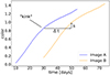 |
Fig. 1. Exemplary noiseless LSN IIP color curves of two lensing images A and B showing a time shift Δt and a shift in color s due to extinction. |
Following the findings in Suyu et al. (2020), we would need cosmology grade time-delay measurements with uncertainties ≲5% of about 20 spatially resolved LSNe Ia with time delays longer than 20 days and including microlensing effects to determine H0 with an uncertainty of ∼1%. We further impose the assumption of ∼3% lens mass modeling uncertainties as well as ∼3% lens environment uncertainties. This is realistic when spatially resolved kinematics of the foreground lens are available (Yıldırım et al. 2020, 2023). We expect to find more LSNe II than LSNe Ia (Wojtak et al. 2019; Goldstein et al. 2018), mostly of type IIn, during the era of LSST, and we find in HOLISMOKES V that LSNe II are less susceptible to microlensing resulting in less biased time delays, even systems with time-delay precision ≲10% will help to achieve the desired precision on the Hubble constant.
We structure our work as follows: In Sect. 2 we go into detail on dust extinction and the creation of our mock SN IIP color curves. We present our MCMC sampling in Sect. 3 and the results in Sect. 4 applying it to the rest-frame SN mock color curves. After that, we look into the impact of redshift in Sect. 5. We finish this work with a discussion and conclusion in Sect. 6.
2. Type II supernova color curves
de Jaeger et al. (2018) finds that SN II color curves show a characteristic change in their slope within the plateau phase, which lasts from (rest-frame) days of ∼10 to ∼100 after explosion. Before the kink around day 35 (rest-frame) after explosion, the color becomes redder more rapidly than afterwards. This “kink” (as shown in Fig. 1) enables us to do cosmography as well as determine extinction parameters.
In this section, we detail the creation of the mock data used in this work. In Sect. 2.1 we introduce the extinction laws by Cardelli et al. (1989) referred to as Cardelli laws. Sect. 2.2 shows the CSP light curves that we use as archetypical SN IIP light curves. We fit these light curves with orthogonal polynomial functions in Sect. 2.3 to create the mock data in Sect. 2.4.
2.1. Dust extinction and extinction parameters
The multiple images of a lensed supernova are observed in different regions of the lensing galaxy. For that reason, it is necessary to emulate the impact of dust on the colors of the lensed images. For this experiment, we use the Cardelli extinction laws, which provide a flexible model of the extinction in galaxies (Cardelli et al. 1988, 1989). The Cardelli laws consider dust absorption and reemission at longer wavelengths as well as light scattering away from the line of sight. The backscattering of light from surrounding stars into the line of sight is omitted as our source is far away. We further ignore extinction occurring in the Milky Way, as we assume it to be the same for the different lensed images owing to the small angular separation. We remark that the Cardelli laws for mock data creation can be exchanged by any other flexible extinction model in galaxies, such as the more recent extinction laws by Gordon et al. (2023), without impacting the retrieval of the time delay.
We denote the intrinsic magnitude as mλ, 0 and the observed magnitude as mλ at the wavelength λ. The wavelength-dependent extinction coefficient is defined as:
 (1)
(1)
Extinction laws are typically defined as Aλ/AV, for which AV is a normalization defined in the optical at λ ≈ 5500 Å. They can also be expressed via the total-to-selective-extinction ratio (Cardelli et al. 1989):
 (2)
(2)
depending on the color excess:
 (3)
(3)
The Cardelli laws (Cardelli et al. 1988, 1989) are generally defined depending only on RV:
 (4)
(4)
The parametric functions a(x) and b(x), where x = λ−1, are determined analytically from spline fits to measured data in the three wavelength regimes, infrared (IR), optical, and ultraviolet (UV) (Cardelli & Clayton 1988; Clayton & Cardelli 1988). The extinction impacts the color curve via a magnitude shift s (see Fig. 1), which is correlated for the case of multiple color curves.
2.2. Observed light curves
Until today, only two spatially resolved lensed SNe II were observed. The lensed core-collapse SN observed in the galaxy cluster Abell 370 has a single epoch observed, which gives us no opportunity to investigate full light curves (Chen et al. 2023). “SN Refsdal” is not of type IIP, but is a 1987A-like SN II (Kelly et al. 2016a). Therefore, we have to create mock color curves based on measured light curves of unlensed SNe IIP. We based our mock color curves on observed light curves from CSP. The data used in this work from CSP (Anderson et al. 2024) are rest-frame u, g, and r band light curves (see Krisciunas et al. 2017 for the definition of the passbands) for SN2005J, which are shown in Fig. 2. We treated these filters as universally applicable to other facilities, which might be used in the future for follow-up observations in the LSST era. The corresponding rest-frame color curves u − g and u − r, used later in the study, show a strong kink mainly because of the larger brightness decrease in the u band compared to the g and r bands. The impact of redshift will be discussed later in Sect. 6.
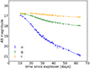 |
Fig. 2. u, g, and r light curves of SN2005J observed by the CSP (Anderson et al. 2024) including examples of orthogonal polynomial fits (solid lines) to the u, g and r band light curves. |
2.3. Light curve model
We first derived a parametrized model of the light curves, which we can use to generate mock light curves and color curves of LSNe IIP. We used orthogonal polynomials as the fitting function C(η,t) that is applied to the observed light curves, where η is the vector of fitting parameters. In addition to the orthogonal polynomial fitting procedure, we tested spline fitting in Appendix A to test the sensitivity of our result to the choice of model.
For the fitting with orthogonal polynomial functions, we considered a linear combination of Legendre polynomials Pn as the functional form C(ηmodel,t) on an interval [tmin, tmax] up to the order of n = 6:
 (5)
(5)
where Pn was defined as:
 (6)
(6)
with substitution u = (2t − tmin − tmax)/(tmax − tmin) to ensure that the Legendre polynomials are orthogonal on an interval t = [tmin, tmax] (with u = [ − 1, 1]) and P0 = 1. The orthogonality interval [tmin, tmax] depends on the time range covered by the color curve of the lensed image observed for the longest period. In our case, we can take either the first or the second image time range, as both are of equal length. This will most likely be the second image for a real measurement, as its light curve can be followed and gathered at an earlier time than the first image. We chose the highest order, n = 6, as it is flexible enough.
The parameter vector is defined as ηmock = (c1,c2,c3,c4,c5,c6,c7)light curve. For the mock data creation, we fited the measured CSP data several times with C(ηmock,t) to ensure reaching the global minimum and selected the fit with the lowest χ2. An example of a light curve fit with up to 6th order orthogonal polynomials to the light curves u, g, and r can be seen in Fig. 2.
2.4. Mock data creation
To generate mock light curves, we assumed systems detected by LSST (Oguri & Marshall 2010) but followed up at a high cadence at a different facility. The parametric SN model, as introduced in Sect. 2.3 was evaluated with an artificial two-day cadence, where each simulated data point can vary around the perfect two-day cadence to simulate realistic observing conditions, adding a value randomly picked from a uniform distribution [−0.1,0.1].
Uncertainties were added following the procedure of Huber et al. (2022) and LSST Science Collaboration (2009), assuming a follow-up facility with a 2 m main mirror. Specifically, at each observational time ti and for each observational band, a random number gi was drawn from a Gaussian with zero mean and standard deviation qi. These numbers were then added to the value determined from the fitted function. The value of qi was set by the signal-to-noise ratio (S/N) of the observed magnitude, which depends on C(ηmock,ti) and the limiting magnitude, which we adopted as one magnitude deeper than the LSST-like 5σ depth (Huber et al. 2019). If C(ηmock,ti) was more than two magnitudes fainter than the 5σ depth, the data point was not generated. Following this approach, we created the mock light curves for the first strongly lensed image A. The mock light curves of the second image, B, were created similarly. However, adding a time and magnitude shift from the filter-dependent extinction and evaluating the model at time steps coinciding with the ones from image A ensures measurements are taken simultaneously for both A and B. For each image, we subtracted the mock light curves in different filters to create the mock color curves dA and dB. The color curve uncertainties σA and σB were calculated by adding the light curve uncertainties in quadrature.
For the main study, we investigated three different scenarios in the mock data creation with SN2005J, which are shown in Table 1:
-
High S/N assuming the uncertainties given by unlensed low redshift observations (Anderson et al. 2024).
-
Low S/N assuming the V band light curve peak of the first image to be at 22 mag and for the second image to be at 23 mag.
-
Low S/N assuming the V band light curve peak of the first image to be at 22 mag and for the second image to be at 23 mag with additionally 35% of the data missing to simulate bad weather conditions and other incidents where observations are not possible.
We used case 1 for method verification, as its high S/N is unrealistic. To mock up case 2 and case 3, we assumed a typical peak absolute brightness at −17 mag in the rest-frame V band (Anderson et al. 2014) for SNe II. In rare cases, the peak absolute magnitude can reach −18 mag. Considering a flat ΛCDM cosmology with H0 = 72 km s−1 Mpc−1 (Bonvin et al. 2017), Ωm = 0.26 and ΩΛ = 0.74 (Oguri & Marshall 2010) and a typical source redshift of lensed SNe II between z = 0.3 and z = 0.6 (Oguri & Marshall 2010), we get the apparent magnitude range of 23.9–25.7 mag. The lens further magnifies this with a typical magnification of μ ≈ 3 for the first image and μ ≈ 1 for the second image (Oguri & Marshall 2010). The first image is, therefore, magnified to around 22.7 magnitudes for the low redshift end, and the second image is not magnified. To keep our cases 2 and 3 realistic but also feasible in terms of observational exposure time, we chose the V band light curve peak of the first image to be at 22 mag and for the second image at 23 mag and adjusted the u, g, and r accordingly, which is still realistic for bright SNe II at the lower redshift boundary. This could also be achievable by observing with a follow-up facility with a main mirror larger than 2 m or deeper 5σ depth than just one magnitude deeper than LSST 5σ depth. To quantify the data loss for scenario 3, we analyzed two years of observations of the quasar RXJ1131-1231 at the 1.2 meter Leonhard Euler Telescope with a two-day cadence from COSMOGRAIL. We find that a loss of ∼35% of observations because of bad weather, downtime of the observatory, or the moon phase is a realistic approximation (Millon et al. 2020b). Reddening due to dust was included, as discussed in Sect. 3.
Investigated mock color curves.
3. Time-delay and extinction retrieval procedure
The light curve model in Eq. (5) will also be used in the MCMC sampling process in this section, using lower orders than the full 6 orders. For the time-delay and extinction parameter retrieval, we use a custom Metropolis-Hastings sampling algorithm (Metropolis et al. 1953) based on the approach of Dunkley et al. (2005) to ensure full control of the sampling. In this section, we introduce our algorithm.
3.1. Likelihood function
The likelihood function assigns a probability  to the sampling parameters
  , and for Gaussian uncertainties the likelihood can be expressed as L = Anormexp(−χ2/2) with Anorm being a normalization factor. During the sampling of our MCMC, as stated in Sect. 3.2 we were just interested in minimizing the χ2 function and do not regard Anorm. To define χ2 in the most general form, we defined the one-dimensional data vectors dA and dB containing the data points of the considered color curves of image A and B. We further considered the model data vectors
  and
and  . The entries of these one-dimensional vectors were defined combining C(η,tj) (Eq. 5) into vector form:
 (7)
(7)
and
 (8)
(8)
where Δt is the time shift, which we sampled together with the parameter vector η and extinction parameters that are related to s. We wrote a general shift s in color between images A and B into this definition, which can be expressed by extinction parameters. Considering generic filters x and y of a color curve x − y, we define the magnitudes m of each image A and B and each filter and get:
 (9)
(9)
For each image (A or B) and filter (x or y), we can write the observed magnitude as:
 (10)
(10)
where m0 is the intrinsic magnitude, Δmlens is the change from lensing magnification, and A is the extinction coefficient. Even though both images have different lensing magnifications, they have the same Δmlens across filters (i.e. Δmlens, A = Δmlens, x, A = Δmlens, y, A and Δmlens, B = Δmlens, x, B = Δmlens, y, B) as lensing is achromatic, neglecting chromatic microlensing effects, which we expect to be small given that the size of photosphere will not change substantially during the plateau phase (Dessart & Hillier 2011), which was also confirmed in our earlier microlensing studies in HOLISMOKES V (Bayer et al. 2021) until around day 30 after explosion. After this epoch, chromatic microlensing might be stronger but still smaller than for SNe Ia. We neglected it in this work, even for later epochs, because of the stable size of the photosphere, but further investigations of microlensing for later epochs of SNe IIP could be of interest in future studies. The additional magnification cancels out, and the equations from Eq. (10) can be inserted into Eq. (9):
![Mathematical equation: $$ \begin{aligned} s =&(m_{0,x} - m_{0,y} - \Delta m_{\mathrm{lens, B} } + \Delta m_{\mathrm{lens, B} } + A_{x,\mathrm{B} } - A_{y,\mathrm{B} })\nonumber \\&- (m_{0,x} - m_{0,y} - \Delta m_{\mathrm{lens, A} } + \Delta m_{\mathrm{lens, A} } + A_{x,\mathrm{A} } - A_{y,\mathrm{A} })\nonumber \\ =&A_{x,\mathrm{B} } - A_{y,\mathrm{B} } - A_{x,\mathrm{A} } + A_{y,\mathrm{A} }\nonumber \\ =&[(a(\lambda _{x}) + \dfrac{b(\lambda _{x})}{R_{V,\mathrm{B} }}) - (a(\lambda _{y}) + \dfrac{b(\lambda _{y})}{R_{V,\mathrm{B} }})] \cdot A_{V,\mathrm{B} } \\&- [(a(\lambda _{x}) + \dfrac{b(\lambda _{x})}{R_{V,\mathrm{A} }}) - (a(\lambda _{y}) + \dfrac{b(\lambda _{y})}{R_{V,\mathrm{A} }})] \cdot A_{V,\mathrm{A} }\nonumber \\ =&[(a(\lambda _{x}) + \dfrac{b(\lambda _{x})}{R_{V}}) - (a(\lambda _{y}) + \dfrac{b(\lambda _{y})}{R_{V}})] \cdot (A_{V,\mathrm{B} }-A_{V,\mathrm{A} }).\nonumber \end{aligned} $$](/articles/aa/full_html/2025/01/aa51824-24/aa51824-24-eq16.gif) (11)
(11)
For the last two steps, we inserted the Cardelli extinction laws from Eq. (4) and fixed RV, A = RV, B = RV = 3.1 which is the standard value for the diffuse interstellar medium (Cardelli et al. 1989). The effective wavelengths used to calculate the parameters a(λ) and b(λ) for the CSP filters are:  ,
,  , and
, and  (Krisciunas et al. 2017).
The final definition of the model data vector for image B was expressed as follows, where AV, B − AV, A is the differential extinction parameter:
![Mathematical equation: $$ \begin{aligned} \begin{array}{l} d_{\mathrm{B} ,i}^{\ \mathrm{model} } = \boldsymbol{C}(\boldsymbol{\eta },t_{i} - \Delta t) + \left[\left(a(\lambda _{x}) + \dfrac{b(\lambda _{x})}{R_{V}}\right)\right.\\ \qquad \qquad \left. - \left(a(\lambda _{y}) + \dfrac{b(\lambda _{y})}{R_{V}}\right)\right] \cdot (A_{V,\mathrm{B} }-A_{V,\mathrm{A} }). \end{array} \end{aligned} $$](/articles/aa/full_html/2025/01/aa51824-24/aa51824-24-eq20.gif) (12)
(12)
The χ2 was defined in the most general form as:
 (13)
(13)
where CD is the covariance matrix. For the simple case of only one color curve, the covariance matrix had only non-zero entries on the main diagonal, where the uncertainties of each color curve data point were calculated by adding the uncertainties of the two respective light-curve data points in quadrature. This also held for using multiple color curves containing only different filters, e.g., for the two color curves u − g and r − i, as it is a good approximation to assume these filters do not correlate. For the case of using color curves containing the same filter, e.g. the two color curves u − g and u − r, we also have entries on the diagonals within the off-diagonal blocks of the matrix, which are not zero. The inverse of the covariance matrix is calculated using the Cholesky decomposition of the numpy.linalg python module (Harris et al. 2020).
3.2. Sampling technique and prior
We started to sample the posterior probability distribution with initial parameters  and (AV, B − AV, A)0 selected with a χ2 non-linear fit of the mock color curves based on a Levenberg-Marquart algorithm as implemented in the optimize.curve_fit function of the python module scipy (Virtanen et al. 2020). The next set of parameters ηi of step i was selected by the walker setting the step size. For the initial chain, we defined the trial probability distribution for taking the next step as a multivariate Gaussian with the identity matrix as the covariance matrix. For the subsequent chain, we used the covariance matrix calculated from the previous chain and scaled it by a constant factor to obtain the trial probability distribution with the desired acceptance rate. This ensured that we had an ideal step size for the walker and an acceptance rate around ∼25% after several chains. We applied a broad uniform prior [−100,100] to the time delay. All other parameters had improper uniform priors. To sample the parameters
  , we followed the Metropolis-Hastings algorithm (Dunkley et al. 2005). We performed a check for convergence as described in Sect. 3.3, and we kept running the chain if convergence was not achieved.
3.3. Convergence testing
During the convergence test, the power spectrum of the samples of each parameter was fitted with the parametric function
 (14)
(14)
from Dunkley et al. (2005). It considered the chain length N, the wave number k* at the turn-over of the power spectrum, the power P0 at wave number k = 0, the Fourier modes j = k(N/(2π)), and an exponent α. A chain converged if the following two criteria were met:
-
j* > 20, with j* = k*(N/(2π)) as the turn-over Fourier mode. This ensured that the minimum wave number kmin was in the regime of white noise P(k)∼k0 indicating that the region of high probability was fully sampled.
-
The convergence ratio r for normalized chains should obey r = (P0/N) < 0.01.
If one of the criteria was not met, we explored an additional 20 000 steps before testing again and repeated this process until convergence was reached. The first 20% of the converged chain was removed as the burn-in phase before convergence testing.
3.4. Polynomial order selection with the Bayesian Information Criterion
We investigated several noise realizations for each mock case to obtain statistically significant results. For case 1 of Table 1, we used 100 noise realizations, and for cases 2 and 3, we used 500 noise realizations, as fluctuations increase with lower S/N. Each noise realization was fitted with different orders of the orthogonal polynomials as presented in Section 2.3, ranging from the linear order 1 to the most complex case of order 6. To select which order to include in the final results, we applied the Bayesian Information Criterion (BIC) to each noise realization and fitted order. The BIC is a simplified criterion for Bayesian model comparison and is defined as:
 (15)
(15)
with the number of data points Ndata, number of free parameters Npar and maximum likelihood  of the noise realization (Schwarz 1978). Choosing the model with the lowest BIC ensures that not only is the best fitting model considered, but also the complexity of each model is taken into account. For the final combination of all investigated noise realizations, we considered the polynomial order of fitting with the lowest BIC value for each realization.
4. Time-delay and extinction retrieval results
In this section, we present the precision and accuracy of our time shift and differential extinction parameter determination method with lensed SN IIP color curves. The input values in the rest-frame mock data creation for all cases in this section were Δt = 16.3 days and AV, B − AV, A = 0.2 mag, which is a realistic value based on the study of the extinction properties of mostly elliptical lensing galaxies (Elíasdóttir et al. 2006). For each of the scenarios 1, 2, and 3 introduced in Sect. 2.4 and Table 1 we investigated the single color curve u − g as well as the combinations of two color curves u − g and u − r. In Appendices A, B, C, and D, we investigated additional scenarios to test the robustness of our method, including other time-shift values.
Before presenting the results, we demonstrate the selection of the orders via the BIC for one case 1 and one case 3 noise realization. All figures about the BIC selection are shown in Appendix E. The high S/N case 1 mock data example with fits of orders 6 down to 2 are shown in Fig. E.1, where we highlight the selected order with a red frame. Further, we list the corresponding BIC values in Table E.1. It is visible that the 5th order fits as well as the 6th order and is favored in the BIC calculation. The lower orders visibly fit worse. For case 3 we show the same orders fit to the mock data in Fig. E.2 as well as the BIC values in Table E.1. For this case, it is not clearly visible which order to favor, but considering the calculated BIC value, the 4th order is selected for this specific noise realization. For each case, this procedure is applied to all noise realizations, resulting in a combination of fits with different orders for the full data set.
The corner plots for mock data case 1 for one color curve u − g and two color curves u − g and u − r are shown in Fig. 3. Cases 2 and 3 are shown in Figs. 4 and 5, respectively. In Fig. 3, both corner plots share the same scale. The corner plots in Figs. 4 and 5 have different scaling, also compared to Fig. 3. The time shifts and differential dust extinctions with uncertainties for all cases are additionally listed in Table 2.
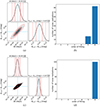 |
Fig. 3. Corner plots of the MCMC chain results and bar plots of selected orders for 100 noise realizations for case 1. The left panels show corner plots of the time shift and differential dust extinction retrieved from 100 noise realizations for case 1. We plot the contours for the 1σ (68%, solid red line) and 2σ (95%, dashed red line) credible intervals for the differential dust extinction AV, B − AV, A and the time delay Δt. The input values in light blue are Δt = 16.3 days and AV, B − AV, A = 0.2 mag. On the right, we show histograms of the selected orthogonal polynomial orders of fitting using the BIC for the corresponding cases on the left. Panel a: Case 1 with one color curve u − g. Panel b: Orders of fitting selected for case 1 with one color curve u − g. Panel c: Case 1 with two color curves u − g and u − r. Panel d: Orders of fitting selected for case 1 with two color curves u − g and u − r. We impose the same order for both color curves. |
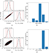 |
Fig. 4. Same as Fig. 3, but for 500 noise realizations for case 2. Panel a: Case 2 with one color curve u − g. Panel b: Orders of fitting selected for case 2 with one color curve u − g. Panel c: Case 2 with two color curves u − g and u − r. Panel d: Orders of fitting selected for case 2 with two color curves u − g and u − r. We impose the same order for both color curves. |
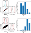 |
Fig. 5. Same as Fig. 3, but for 500 noise realizations for case 3. Panel a: Case 3 with one color curve u − g. Panel b: Orders of fitting selected for case 3 with one color curve u − g. Panel c: Case 3 with two color curves u − g and u − r. Panel d: Orders of fitting selected for case 3 with two color curves u − g and u − r. We impose the same order for both color curves. |
Results of the time-delay and differential dust extinction retrieval for each investigated S/N and color curve scenario.
Considering case 1 for one and two color curves, we can retrieve the time shift and the differential extinction perfectly with relative uncertainties down to the 1% level for typical delays and extinctions, which proves the functionality of the method. Furthermore, combining multiple color curves helps with constraining both the time delay and the differential dust extinction. For high S/N data in case 1, only high orders of the orthogonal polynomial fitting are selected via the BIC, as shown in Figs. 3b and 3d.
When adjusting the S/N down for case 2, the result gets less precise, as expected. Considering only the u − g color curve, we cannot retrieve the time delay precisely enough to be of cosmology grade as defined in Sect. 1, unless the delays are longer than ∼35 days, to reach an uncertainty ≲10% per lens system. This gets even less precise for the most realistic case 3, including 35% data loss, where uncertainties reach ∼5–6 days. AV, B − AV, A cannot be constrained to better than ∼0.7 mag with a single color curve in low S/N cases. By including the second color curve u − r, the constraint on the differential dust extinction is improved substantially to < 0.1 mag in precision, which helps break the degeneracy between Δt and AV, B − AV, A and decreases the time delay uncertainty down to ∼1 day. For the lower S/N cases with one color curve, lower orders of fitting are selected via the BIC because the higher uncertainties of the mock data leave more freedom in the functional form of the fit. This gets shifted to higher orders again when a second color curve is taken into account, as it sets more constraints on the fit.
5. Inference for non-zero redshift
Up to now, we investigated rest-frame photometry in the CSP filters u, g, and r. In reality, we would observe most lensed SNe II at redshifts around z = 0.6 (Oguri & Marshall 2010). Assuming a redshift of z = 0.6, the rest-frame u, g, and r bands would shift roughly into the observed r, i, and z bands, respectively. In this section, we investigate how the shape of the kink is affected with the help of K-corrections and the rest-frame UV color curves of the Ultra Violet Optical Telescope (UVOT) on the Neil Gehrels Swift Observatory (SWIFT) (Gehrels et al. 2004; Roming et al. 2005) SNe, which would be approximately observed in the u and g band for z = 0.6.
5.1. K-corrections
For applying K-corrections, we need spectra, but for the CSP and SWIFT data, we have no spectra available to cover the rest-frame UV. We, therefore, use publicly available model spectra of SN IIP with temporal evolution created by Dessart et al. (2013)1. We applied the K-correction to the photometry according to Hogg et al. (2002) by adding K to the rest-frame magnitude in the rest-frame filter to retrieve the observed magnitude in the observed filter given the function:
![Mathematical equation: $$ \begin{aligned} \begin{array}{l} K = -2.5 \log \left[\frac{1}{1+z} \frac{\int \lambda _{\mathrm{obs} } \ f(\lambda _{\mathrm{obs} }) \ R(\lambda _{\mathrm{obs} }) \ \mathrm{d} \lambda _{\mathrm{obs} }}{\int \lambda _{\mathrm{obs} } \ g^{R}(\lambda _{\mathrm{obs} }) \ R(\lambda _{\mathrm{obs} }) \ \mathrm{d} \lambda _{\mathrm{obs} }} \times \right. \\ \qquad \qquad \qquad \qquad \left. \frac{\int \lambda _{\mathrm{rest} } \ g^{Q}(\lambda _{\mathrm{rest} }) \ Q(\lambda _{\mathrm{rest} }) \ \mathrm{d} \lambda _{\mathrm{rest} }}{\int \lambda _{\mathrm{rest} } \ f((1+z) \lambda _{\mathrm{rest} }) \ Q(\lambda _{\mathrm{rest} }) \ \mathrm{d} \lambda _{\mathrm{rest} }} \right], \end{array} \end{aligned} $$](/articles/aa/full_html/2025/01/aa51824-24/aa51824-24-eq39.gif) (16)
(16)
with the observed wavelength λobs, observed flux f(λobs), transmission function of the filter in the observed frame R(λobs), rest-frame wavelength λrest, rest-frame flux f(λrest), and transmission function of the filter in the rest-frame Q(λrest). gR(λobs) and gQ(λrest) are the spectral flux densities for a magnitude of zero in the AB system in the observed frame and the rest-frame, respectively. We inserted the LSST u and g bands for the rest-frame transmission functions and the r and i bands for the observed-frame transmission function, as u and g are roughly shifted into these bands for z = 0.6. The resulting color curves are shown in Fig. 6.
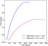 |
Fig. 6. Rest-frame u − g color curve and corresponding redshifted r − i color curve created from model spectra. The kink of the rest-frame color curve is slightly weakened by the K-correction. |
The strength of the kink was defined by the change in the slopes of the color curve before and after the kink. The stronger the change, the stronger the kink. Applying the K-correction, the kink of the color curve, which occurs in this case around day 95, is slightly weakened. As this change is not too drastic, we expect that redshifted SNe IIP color curves still exhibit a sufficiently strong kink for our method to work, especially when combining multiple color curves. To include redshifted color curves using the observed u and g bands, we will next investigate the evolution of rest-frame UV color curves.
5.2. Rest-frame UV color curves
To estimate how rest-frame UV color curves are redshifted into the range of LSST bands, we investigated the UV color curves with the UVOT filters uvw1 and b of the two SWIFT SNe SN2020jfo and SN2017eaw. We had to limit the SWIFT light curves to the UVOT rest-frame uvw1 and b bands, as only these two bands have good coverage of the epochs around the kink observed in the color curves. The data for SN2020jfo was taken from Sollerman et al. (2021) and for SN2017eaw from Szalai et al. (2019). The rest-frame uvw1 − b color curves of both SNe in Fig. 7 show a particularly strong kink. We found that this results from the long wavelength tail of the uvw1 filter reaching into the visible spectral range.
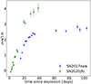 |
Fig. 7. uvw1 − b color curves of SWIFT SNe SN2017eaw (blue) (Szalai et al. 2019) and SN2020jfo (green) (Sollerman et al. 2021). |
We investigated how cutting this uvw1 filter tail away at ∼3347.5 Å to create a filter uvw1* affects the kink in color curves, by creating artificial color curves uvw1 − b and uvw1* − b with the spectra by Dessart et al. (2013). The resulting color curves are shown in Fig. 8.
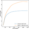 |
Fig. 8. Color curves uvw1 − b (blue) and uvw1* − b (orange) created with the Dessart et al. (2013) model spectra using the SWIFT filters uvw1, b, and the modified uvw1*, where the red tail has been cut. The color curve uvw1* − b still shows a sufficiently strong kink for our time delay method to work. |
uvw1* − b shows a weaker kink than uvw1 − b, but still stronger than the u − g rest-frame color curve from Fig. 6. We, therefore, conclude that bluer colors tend to show even stronger kinks for SNe IIP, which helps us constrain the time delay for redshifted SNe IIP.
6. Discussion and conclusion
We developed a Metropolis-Hastings MCMC-based method of fitting lensed SN IIP color curves with orthogonal polynomial functions to retrieve the time delay Δt and the differential dust extinction AV, B − AV, A between two lensing images A and B.
In the high-S/N limit, the method works flawlessly using either one or two color curves, and the time delay Δt and the differential dust extinction AV, B − AV, A can be retrieved precisely without bias. We note that AV of each individual image is only determined precisely for the case of one color curve, assuming the knowledge of the macro-magnification. Orthogonal polynomial functions are flexible enough to fit data that may follow different functional forms.
Considering more realistic cases with low S/N and data loss because of observational constraints, the inference of Δt and especially with AV, B − AV, A is more uncertain. For one color curve, the precision of the time delay degrades to ≳3 days. Adding the information of a third light curve band helps constrain both parameters. Fitting two color curves calculated from light curves in 3 bands gives more constraints on AV, B − AV, A helping to break the degeneracy between the time delay and the differential dust extinction. This also has the advantage that absolute magnification cancels out between the two color curves, assuming we choose the correct RV and extinction law during sampling.
We are aware that our assumption of knowing perfectly RV and the correct extinction law is strong and simplifies the determination of Δt and AV, B − AV, A. We show in Appendix D that for combining two realistic mock color curves with low S/N and data loss using a different extinction law, Δt can still be determined precisely and without bias, which is the main objective of this work. The accuracy of AV, B − AV, A depends more on RV than on the specific extinction law in the wavelength range of the LSST filters.
Despite all the measures we take to create realistic mock color curves, we anticipate some additional uncertainties in real data. Three additional nuisance effects may be expected for real data: the decrease in S/N because of the additional shot noise from the host galaxy of the SN and the lens, photometric errors due to the blending of the SN images, and the impact of the seeing on the above two effects. The influence of these effects will have to be studied in the future when more observed lensed SNe IIP are available. Another simplification of the existing framework is the use of a non-redshifted reddening. This should not impact our results heavily within the obtained uncertainties, as the observed bands probe a region of the extinction laws that is monotonically decreasing, and the lens will be likely at low redshifts around z = 0.2 − 0.4 (Oguri & Marshall 2010).
Considering all rest-frame cases presented in Sect. 4 as well as Appendix A, B, and C, we can determine several trends:
-
The more color curves we take into account during sampling the better we can determine AV, B − AV, A, which also results in a better constraint on the time delay, as different color curves can help to break the degeneracy in Δt and AV, B − AV, A.
-
The data needed for this method to work for rest-frame u, g, and r band should ideally be dedicated follow-up multiband observation with a cadence of not more than two rest-frame days and a depth that is 1 mag deeper than LSST to have a high enough S/N for typical lensed-SN redshifts and magnifications (Huber et al. 2022). In addition to dedicated follow-up observations, the upcoming space-based survey telescope Roman might also have a high enough cadence of ∼5 observed frame days, high resolution, and sensitivity. One should note it is covering the NIR starting roughly at the LSST r band wavelength range, limiting the amount of useful SNe IIP coverage to high-redshift ones as the color curves of redder rest-frame filters show almost no kink, especially considering the range of expected uncertainties (Pierel et al. 2021). Furthermore, we should remember that Roman is a survey that is more likely to cover a lensed SN by chance rather than collecting dedicated data through a follow-up target of opportunity-based observation.
-
The K-correction investigation in Sect. 5 of rest-frame UV bands redshifted into the LSST bands u, g, r, and i, shows strong enough kinks to be usable for our MCMC retrieval technique. Bluer colors tend to show stronger kinks for SNe IIP. Hence, the redshift of a lensed SN IIP helps us to get better time-delay measurements with ground-based photometry.
-
A higher S/N ratio, a larger number of considered color curves, and lower data loss result in a higher selected order of fitting for the orthogonal polynomials as the data impose higher constraints.
-
Cluster-lensed SNe IIP are less susceptible to differential dust extinction, as dust occurs more in star formation regions, and the lensing images might not be in the line of sight of the lens. This makes cluster-lensed SNe IIP desirable for our time-delay retrieval method using color curves as they could provide more precise results compared to galaxy-scale lensed SNe IIP.
The method is precise enough for obtaining cosmology grade time delays for gravitationally lensed SNe IIP with realistic uncertainties around ∼1.0 day. For 20 SNe IIP with time delays longer than 20 days, we will thus be able to constrain H0 with an uncertainty of ∼1% during the era of LSST (Suyu et al. 2020). Comparing the results of this work to our previous paper HOLISMOKES V (Bayer et al. 2021), which uses a combination of absorption lines within spectra of LSNe IIP, we achieve a similar accuracy and precision of ∼1.0 day.
Acknowledgments
We thank F. Dux, M. Millon, and F. Courbin for discussions on realistic data loss in observations, and J. Anderson and T. de Jaeger for providing us with the observational data of SN2005J and other SNe of the CSP for developing and testing our code, and E. Fitzpatrick for discussions on dust extinction laws. We also thank R. Cañameras for his feedback on our work and the anonymous referee for constructive comments. We acknowledge the use of public data from the Swift data archive. We thank the Max Planck Society for support through the Max Planck Research Group and Fellowship for SHS. This project has received funding from the European Research Council (ERC) under the European Union’s Horizon 2020 research and innovation programme (LENSNOVA: grant agreement No. 771776; COSMICLENS: grant agreement No. 787886). This research is supported in part by the Excellence Cluster ORIGINS, which is funded by the Deutsche Forschungsgemeinschaft (DFG, German Research Foundation) under Germany’s Excellence Strategy – EXC-2094 – 390783311.
References
- Anand, G. S., Riess, A. G., Yuan, W., et al. 2024, ApJ, 966, 89 [NASA ADS] [CrossRef] [Google Scholar]
- Anderson, J. P., González-Gaitán, S., Hamuy, M., et al. 2014, ApJ, 786, 67 [Google Scholar]
- Anderson, J. P., Contreras, C., Stritzinger, M. D., et al. 2024, A&A, 692, A95 [NASA ADS] [CrossRef] [EDP Sciences] [Google Scholar]
- Arendse, N., Dhawan, S., Sagués Carracedo, A., et al. 2024, MNRAS, 531, 3509 [NASA ADS] [CrossRef] [Google Scholar]
- Bayer, J., Huber, S., Vogl, C., et al. 2021, A&A, 653, A29 [NASA ADS] [CrossRef] [EDP Sciences] [Google Scholar]
- Birrer, S., Treu, T., Rusu, C. E., et al. 2019, MNRAS, 484, 4726 [Google Scholar]
- Birrer, S., Shajib, A. J., Galan, A., et al. 2020, A&A, 643, A165 [NASA ADS] [CrossRef] [EDP Sciences] [Google Scholar]
- Bonvin, V., Courbin, F., Suyu, S. H., et al. 2017, MNRAS, 465, 4914 [NASA ADS] [CrossRef] [Google Scholar]
- Bonvin, V., Chan, J. H. H., Millon, M., et al. 2018, A&A, 616, A183 [NASA ADS] [CrossRef] [EDP Sciences] [Google Scholar]
- Buchner, J. 2014, Stat. Comput., 26, 383 [Google Scholar]
- Buchner, J. 2019, PASP, 131, 108005 [Google Scholar]
- Buchner, J. 2021, JOSS, 6, 3001 [NASA ADS] [CrossRef] [Google Scholar]
- Cardelli, J. A., & Clayton, G. C. 1988, AJ, 95, 516 [NASA ADS] [CrossRef] [Google Scholar]
- Cardelli, J. A., Clayton, G. C., & Mathis, J. S. 1988, ApJ, 329, L33 [NASA ADS] [CrossRef] [Google Scholar]
- Cardelli, J. A., Clayton, G. C., & Mathis, J. S. 1989, ApJ, 345, 245 [Google Scholar]
- Chen, G. C. F., Fassnacht, C. D., Suyu, S. H., et al. 2019, MNRAS, 490, 1743 [NASA ADS] [CrossRef] [Google Scholar]
- Chen, W., Kelly, P., Oguri, M., et al. 2023, Am. Astron. Soc. Meet. Abstr., 55, 432.08 [Google Scholar]
- Clayton, G. C., & Cardelli, J. A. 1988, AJ, 96, 695 [NASA ADS] [CrossRef] [Google Scholar]
- Courbin, F., Bonvin, V., Buckley-Geer, E., et al. 2018, A&A, 609, A71 [NASA ADS] [CrossRef] [EDP Sciences] [Google Scholar]
- de Jaeger, T., Anderson, J. P., Galbany, L., et al. 2018, MNRAS, 476, 4592 [NASA ADS] [CrossRef] [Google Scholar]
- Dessart, L., & Hillier, D. J. 2006, A&A, 447, 691 [NASA ADS] [CrossRef] [EDP Sciences] [Google Scholar]
- Dessart, L., & Hillier, D. J. 2009, AIP Conf. Ser., 1111, 565 [NASA ADS] [CrossRef] [Google Scholar]
- Dessart, L., & Hillier, D. J. 2011, MNRAS, 410, 1739 [NASA ADS] [Google Scholar]
- Dessart, L., Blondin, S., Brown, P. J., et al. 2008, ApJ, 675, 644 [NASA ADS] [CrossRef] [Google Scholar]
- Dessart, L., Hillier, D. J., Waldman, R., & Livne, E. 2013, MNRAS, 433, 1745 [NASA ADS] [CrossRef] [Google Scholar]
- Di Valentino, E., Mena, O., Pan, S., et al. 2021, Class. Quant. Grav., 38, 153001 [NASA ADS] [CrossRef] [Google Scholar]
- Dobler, G., & Keeton, C. R. 2006, ApJ, 653, 1391 [NASA ADS] [CrossRef] [Google Scholar]
- Dunkley, J., Bucher, M., Ferreira, P., Moodley, K., & Skordis, C. 2005, MNRAS, 356, 925 [NASA ADS] [CrossRef] [Google Scholar]
- Eigenbrod, A., Courbin, F., Vuissoz, C., et al. 2005, A&A, 436, 25 [NASA ADS] [CrossRef] [EDP Sciences] [Google Scholar]
- Elíasdóttir, Á., Hjorth, J., Toft, S., Burud, I., & Paraficz, D. 2006, ApJS, 166, 443 [Google Scholar]
- Freedman, W. L. 2021, ApJ, 919, 16 [NASA ADS] [CrossRef] [Google Scholar]
- Freedman, W. L., Madore, B. F., Hatt, D., et al. 2019, ApJ, 882, 34 [Google Scholar]
- Freedman, W. L., Madore, B. F., Hoyt, T., et al. 2020, ApJ, 891, 57 [Google Scholar]
- Frye, B., Pascale, M., Cohen, S., et al. 2023, TNSAN, 96, 1 [NASA ADS] [Google Scholar]
- Frye, B. L., Pascale, M., Pierel, J., et al. 2024, ApJ, 961, 171 [NASA ADS] [CrossRef] [Google Scholar]
- Gayathri, V., Healy, J., Lange, J., et al. 2021, ApJ, 908, L34 [NASA ADS] [CrossRef] [Google Scholar]
- Gehrels, N., Chincarini, G., Giommi, P., et al. 2004, ApJ, 611, 1005 [Google Scholar]
- Gilman, D., Birrer, S., & Treu, T. 2020, A&A, 642, A194 [NASA ADS] [CrossRef] [EDP Sciences] [Google Scholar]
- Goldstein, D. A., & Nugent, P. E. 2017, ApJ, 834, L5 [Google Scholar]
- Goldstein, D. A., Nugent, P. E., Kasen, D. N., & Collett, T. E. 2018, ApJ, 855, 22 [NASA ADS] [CrossRef] [Google Scholar]
- Goobar, A., Amanullah, R., Kulkarni, S. R., et al. 2017, Science, 356, 291 [Google Scholar]
- Goobar, A. A., Johansson, J., Dhawan, S., et al. 2022, TNSAN, 180, 1 [NASA ADS] [Google Scholar]
- Gordon, K. D., Clayton, G. C., Decleir, M., et al. 2023, ApJ, 950, 86 [CrossRef] [Google Scholar]
- Grillo, C., Pagano, L., Rosati, P., & Suyu, S. H. 2024, A&A, 684, L23 [NASA ADS] [CrossRef] [EDP Sciences] [Google Scholar]
- Hamuy, M., Folatelli, G., Morrell, N. I., et al. 2006, PASP, 118, 2 [NASA ADS] [CrossRef] [Google Scholar]
- Harris, C. R., Millman, K. J., van der Walt, S. J., et al. 2020, Nature, 585, 357 [NASA ADS] [CrossRef] [Google Scholar]
- Hogg, D. W., Baldry, I. K., Blanton, M. R., & Eisenstein, D. J. 2002, arXiv e-prints [arXiv:astro-ph/0210394] [Google Scholar]
- Huber, S., & Suyu, S. H. 2024, A&A, 692, A132 [NASA ADS] [CrossRef] [EDP Sciences] [Google Scholar]
- Huber, S., Suyu, S. H., Noebauer, U. M., et al. 2019, A&A, 631, A161 [NASA ADS] [CrossRef] [EDP Sciences] [Google Scholar]
- Huber, S., Suyu, S. H., Noebauer, U. M., et al. 2021, A&A, 646, A110 [NASA ADS] [CrossRef] [EDP Sciences] [Google Scholar]
- Huber, S., Suyu, S. H., Ghoshdastidar, D., et al. 2022, A&A, 658, A157 [NASA ADS] [CrossRef] [EDP Sciences] [Google Scholar]
- Kelly, P. 2015, IAU General Assembly, 29, 2251986 [NASA ADS] [Google Scholar]
- Kelly, P. L., Brammer, G., Selsing, J., et al. 2016a, ApJ, 831, 205 [NASA ADS] [CrossRef] [Google Scholar]
- Kelly, P. L., Rodney, S. A., Treu, T., et al. 2016b, ApJ, 819, L8 [NASA ADS] [CrossRef] [Google Scholar]
- Kelly, P. L., Rodney, S., Treu, T., et al. 2023, Science, 380, abh1322 [NASA ADS] [CrossRef] [Google Scholar]
- Krisciunas, K., Contreras, C., Burns, C. R., et al. 2017, AJ, 154, 211 [NASA ADS] [CrossRef] [Google Scholar]
- Li, W., Leaman, J., Chornock, R., et al. 2011, MNRAS, 412, 1441 [NASA ADS] [CrossRef] [Google Scholar]
- Li, S., Riess, A. G., Casertano, S., et al. 2024, ApJ, 966, 20 [NASA ADS] [CrossRef] [Google Scholar]
- Liu, Y., & Oguri, M. 2024, arXiv e-prints [arXiv:2402.13476] [Google Scholar]
- LSST Science Collaboration (Abell, P. A., et al.) 2009, arXiv e-prints, [arXiv:0912.0201] [Google Scholar]
- Metropolis, N., Rosenbluth, A. W., Rosenbluth, M. N., Teller, A. H., & Teller, E. 1953, J. Chem. Phys., 21, 1087 [Google Scholar]
- Millon, M., Galan, A., Courbin, F., et al. 2020a, A&A, 639, A101 [NASA ADS] [CrossRef] [EDP Sciences] [Google Scholar]
- Millon, M., Courbin, F., Bonvin, V., et al. 2020b, A&A, 642, A193 [NASA ADS] [CrossRef] [EDP Sciences] [Google Scholar]
- Mukherjee, S., Lavaux, G., Bouchet, F. R., et al. 2021, A&A, 646, A65 [NASA ADS] [CrossRef] [EDP Sciences] [Google Scholar]
- Oguri, M., & Marshall, P. J. 2010, MNRAS, 405, 2579 [NASA ADS] [Google Scholar]
- Palmese, A., Kaur, R., Hajela, A., et al. 2024, Phys. Rev. D, 109, 063508 [CrossRef] [Google Scholar]
- Pascale, M., Frye, B. L., Pierel, J. D. R., et al. 2024, ApJ, submitted [arXiv:2403.18902] [Google Scholar]
- Pesce, D. W., Braatz, J. A., Reid, M. J., et al. 2020, ApJ, 891, L1 [Google Scholar]
- Pierel, J. D. R., Rodney, S., Vernardos, G., et al. 2021, ApJ, 908, 190 [NASA ADS] [CrossRef] [Google Scholar]
- Pierel, J. D. R., Frye, B. L., Pascale, M., et al. 2024, ApJ, 967, 50 [NASA ADS] [CrossRef] [Google Scholar]
- Planck Collaboration VI. 2020, A&A, 641, A6 [NASA ADS] [CrossRef] [EDP Sciences] [Google Scholar]
- Refsdal, S. 1964, MNRAS, 128, 307 [NASA ADS] [CrossRef] [Google Scholar]
- Riess, A. G., Breuval, L., Yuan, W., et al. 2022, ApJ, 938, 36 [NASA ADS] [CrossRef] [Google Scholar]
- Riess, A. G., Anand, G. S., Yuan, W., et al. 2024, ApJ, 962, L17 [NASA ADS] [CrossRef] [Google Scholar]
- Rodney, S. A., Brammer, G. B., Pierel, J. D. R., et al. 2021, Nat. Astron., 5, 1118 [NASA ADS] [CrossRef] [Google Scholar]
- Roming, P. W. A., Kennedy, T. E., Mason, K. O., et al. 2005, Space Sci. Rev., 120, 95 [Google Scholar]
- Rusu, C. E., Wong, K. C., Bonvin, V., et al. 2020, MNRAS, 498, 1440 [Google Scholar]
- Schwarz, G. 1978, Ann. Stat., 6, 461 [Google Scholar]
- Shajib, A. J., Birrer, S., Treu, T., et al. 2020, MNRAS, 494, 6072 [Google Scholar]
- Sluse, D., Rusu, C. E., Fassnacht, C. D., et al. 2019, MNRAS, 490, 613 [NASA ADS] [CrossRef] [Google Scholar]
- Sollerman, J., Yang, S., Schulze, S., et al. 2021, A&A, 655, A105 [NASA ADS] [CrossRef] [EDP Sciences] [Google Scholar]
- Soltis, J., Casertano, S., & Riess, A. G. 2021, ApJ, 908, L5 [Google Scholar]
- Suyu, S. H., Bonvin, V., Courbin, F., et al. 2017, MNRAS, 468, 2590 [Google Scholar]
- Suyu, S. H., Huber, S., Cañameras, R., et al. 2020, A&A, 644, A162 [NASA ADS] [CrossRef] [EDP Sciences] [Google Scholar]
- Szalai, T., Vinkó, J., Könyves-Tóth, R., et al. 2019, ApJ, 876, 19 [Google Scholar]
- Treu, T., Agnello, A., Baumer, M. A., et al. 2018, MNRAS, 481, 1041 [NASA ADS] [CrossRef] [Google Scholar]
- Verde, L., Treu, T., & Riess, A. G. 2019, Nat. Astron., 3, 891 [Google Scholar]
- Virtanen, P., Gommers, R., Oliphant, T. E., et al. 2020, Nat. Methods, 17, 261 [Google Scholar]
- Vogl, C., Kerzendorf, W. E., Sim, S. A., et al. 2020, A&A, 633, A88 [NASA ADS] [CrossRef] [EDP Sciences] [Google Scholar]
- Wojtak, R., Hjorth, J., & Gall, C. 2019, MNRAS, 487, 3342 [Google Scholar]
- Wong, K. C., Suyu, S. H., Chen, G. C. F., et al. 2020, MNRAS, 498, 1420 [Google Scholar]
- Yıldırım, A., Suyu, S. H., & Halkola, A. 2020, MNRAS, 493, 4783 [Google Scholar]
- Yıldırım, A., Suyu, S. H., Chen, G. C. F., & Komatsu, E. 2023, A&A, 675, A21 [NASA ADS] [CrossRef] [EDP Sciences] [Google Scholar]
Appendix A: Fitting with a different model
For our main study, we used the same functional form (orthogonal polynomials) to generate and fit the mock data. In this appendix, we explore if the method might produce model-induced biased results if the mock data is created with a spline model and sampled with orthogonal polynomials. Further, we do not expect real data to follow the behavior of orthogonal polynomials, nor a spline, and we want to ensure that the model used during sampling is flexible enough to fit the data based on a different model.
For the mock data creation, we created a spline function consisting of two third-order polynomials connected at one knot tknot defined as:
 (A.1)
(A.1)
with the additional condition of the same slope at the knot:
 (A.2)
(A.2)
The collective parameter vectors were defined as  and
and  for C1(η1, t). With the slope condition, we can eliminate the parameter c7 and express it via the other parameters:
 (A.3)
(A.3)
We inserted Eq. A.3 into Eq. A.1:
![Mathematical equation: $$ \begin{aligned} C(\boldsymbol{\eta },t) = {\left\{ \begin{array}{ll} C_{1}(\boldsymbol{\eta }_{1},t) = c_{1} t^{3} + c_{2} t^{2}\\ \ \ \ \ \ \ \ \ \ \ \ \ \ \ \ \ \ \ + c_{3} t + c_{4} \ \ \ \ \ \ \ \ \ \ \ \ \ \ \ \ \ \ \ \text{ for} \ t \le t_{\mathrm{knot} }\\ C_{2}(\boldsymbol{\eta },t) \ \ = c_{5} t^{3} + c_{6} t^{2} \\ \ \ \ \ \ \ \ \ \ \ \ \ \ \ \ \ \ \ + [3t_{\mathrm{knot} }^{2}(c_{1}-c_{5}) \\ \ \ \ \ \ \ \ \ \ \ \ \ \ \ \ \ \ \ + 2t_{\mathrm{knot} }(c_{2}-c_{6})\\ \ \ \ \ \ \ \ \ \ \ \ \ \ \ \ \ \ \ + c_{3}] t + (c_{1}-c_{5}) t_{\mathrm{knot} }^{3}\\ \ \ \ \ \ \ \ \ \ \ \ \ \ \ \ \ \ \ + (c_{2}-c_{6}) t_{\mathrm{knot} }^{2} \\ \ \ \ \ \ \ \ \ \ \ \ \ \ \ \ \ \ \ + (c_{3}-[3t_{\mathrm{knot} }^{2}(c_{1}-c_{5})\\ \ \ \ \ \ \ \ \ \ \ \ \ \ \ \ \ \ \ + 2t_{\mathrm{knot} }(c_{2}-c_{6})\\ \ \ \ \ \ \ \ \ \ \ \ \ \ \ \ \ \ \ + c_{3}]) t_{\mathrm{knot} } + c_{4} \ \ \ \ \ \ \ \ \ \ \ \text{ for} \ t > t_{\mathrm{knot} }, \\ \end{array}\right.} \end{aligned} $$](/articles/aa/full_html/2025/01/aa51824-24/aa51824-24-eq45.gif) (A.4)
(A.4)
and redefined the parameter vector  . Besides the change in generating mock data, we followed the same approach as described in Sect. 3.
We first investigated high S/N with only one color curve u − g and 100 noise realizations, as this simple case will show most easily if a bias occurs. The resulting corner plot is shown in Fig. A.1 for which only the 6th order was selected by the BIC. It has a slight bias in the time shift and the differential extinction, although the bias in Δt is only 0.03 days, which is at the subpercent level for most lensed SN systems of interest in our program.
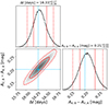 |
Fig. A.1. Corner plot for mock data created with spline fitting, including 100 noise realizations with high S/N. The initial input values shown in light blue are Δt = 16.3 days and AV, B − AV, A = 0.2 mag. |
We further checked the case of low S/N with one color curve u − g and 500 noise realizations. Because of the low S/N, the result shown in Fig. A.2 is unbiased within the uncertainties. The selected orders are shown in the bar plot in A.3
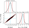 |
Fig. A.2. Corner plot for mock data created with spline fitting including 500 noise realizations with low S/N. The initial input values shown in light blue are Δt = 16.3 days and AV, B − AV, A = 0.2 mag. |
This proves that for the realistic cases with low S/N, we can retrieve unbiased results even with different models used in mock data creation and sampling.
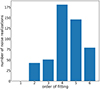 |
Fig. A.3. Histogram of the selected orthogonal polynomial orders of fitting using the BIC for the low S/N mock data created with spline fitting. |
Appendix B: Completely degenerate case
Another test of the functionality of our code was to create a mock color curve case that was perfectly linear in both images and tried to retrieve a time delay with our method. We expected that the preferred order selected with the BIC of the orthogonal polynomials would be one, and the distribution in the time shift and differential extinction would be completely degenerate. As it can be seen in Fig. B.1, we can retrieve an exact degeneracy up to the borders of the prior, and during the BIC selection, only order one was selected. Even if AV, B − AV, A has no prior boundaries as it has an unbound uniform prior, it is limited by the boundaries of the prior for Δt. This test shows that for featureless (linear) color curves, our color curve time-delay determination breaks down.
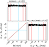 |
Fig. B.1. Corner plot combining 100 noise realizations of perfect linear mock color curves u − g. Because of the linearity of the mock data, a complete degeneracy is retrieved. |
Appendix C: Different shifts
Our main study focused only on one time shift Δt = 16.3 days. Here, we also investigated two cases with Δtsmall = 0.5 days and Δtlarge = 50 days to check that any low or high time shift can be retrieved. We did not explore time shifts longer than 50 days, as these can also be detected by eye and shifted manually into the range of Δt< 50 days, which ensures that our code can be applied to any time shift. To create the two plots in Fig. C.1 and Fig. C.2, we followed the same procedure as explained in Sect. 3 with 100 noise realizations and high S/N data, just switching out the time shift in the mock data creation to Δtsmall = 0.5 days and Δtlarge = 50 days. For both new time shifts, a similar distribution of the fitting orders as for case 1 with one color curve shown in Fig. 3b was selected.
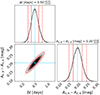 |
Fig. C.1. Corner plot of 100 noise realizations of high S/N mock data with Δtsmall = 0.5 days and AV, B − AV, A = 0.2 mag |
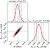 |
Fig. C.2. Corner plot of 100 noise realizations of high S/N mock data with Δtlarge = 50.0 days and AV, B − AV, A = 0.2 mag |
For both cases, we can retrieve the time delay and differential dust extinction, as well as for case 1 considered in Sect. 4 using only one color curve u − g, which confirms that the code can be applied to any time shift within 0.5 days to 50 days.
Besides all the testing presented here in the appendix, we also used the nested sampling Monte Carlo algorithm MLFriends (Buchner 2014, 2019) from the UltraNest2 package (Buchner 2021) with our technique and obtained the same results, confirming that our sampling code works correctly. Using our own code gave us even faster results because we did not calculate the Bayesian evidence.
Appendix D: Different extinction laws for mock data and sampling
In the main study, we knew and adopted the correct extinction law to sample the color curves. In reality, this will not be the case, and we might assume RV wrongly or use an extinction law not fitting the real data. Therefore, we tested three additional cases with 100 noise realizations for the realistic case of low S/N with 35% data loss for two color curves u − g and u − r. All three cases were still based on the same mock data as explained in Sect. 2.4.
The first test case, T1, set RV= 2.0 for the sampling. The second case, T2, used RV= 5.0 for sampling. For both T1 and T2, we still used Cardelli extinction laws in the sampling process described in Sect. 3. The third test case, T3, applied more recent extinction laws from Gordon et al. (2023), referred to as Gordon laws, in the sampling, but kept RV= 3.1. The Gordon laws have a similar approach as the Cardelli laws in Eq. 4, but are based on more recent measurements for a(x) and b(x) and are normalized differently:
 (D.1)
(D.1)
The resulting corner plots for T1, T2, and T3 are shown in Fig. D.1, D.2, and D.3 respectively. The orthogonal polynomial orders selected via the BIC for all cases follow a similar distribution, as shown in Fig. 5d. For T1 and T2, the time delays have a bias of 0.1-0.2 days, which for delays > 20 days are still at the < 1% level. That is within the tolerance to achieve a 1% H0 measurement. For short delays, the RV value has a relatively larger impact on the accuracy of the delays. Therefore, RV should be incorporated in the measurement of the delays. In both test cases of T1 and T2, AV, B − AV, A can not be sampled correctly anymore, which is to be expected considering an incorrect RV value.
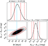 |
Fig. D.1. Corner plot of 100 noise realizations of low S/N mock data with 35% data loss and with input time delay Δt = 16.3 days for combining u − g and u − r color curves setting RV = 2.0 during MCMC sampling. |
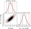 |
Fig. D.2. Corner plot of 100 noise realizations of low S/N mock data with 35% data loss and with input time delay Δt = 16.3 days for combining u − g and u − r color curves setting RV = 5.0 during MCMC sampling. |
For T3, both Δt and AV, B − AV, A are retrieved unbiased and precisely because the Cardelli extinction laws and the Gordon laws follow a similar behavior in the considered wavelength range and differ only a bit in the a(x) and b(x) values. If the data covered the ultraviolet or infrared wavelength range of the extinction laws, the results would deviate more. The same would occur if extinction laws that do not follow the Cardelli laws as closely as the Gordon laws would be applied.
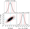 |
Fig. D.3. Corner plot of 100 noise realizations of low S/N mock data with 35% data loss and with input time delay Δt = 16.3 days for combining u − g and u − r color curves using extinction laws by Gordon et al. (2023) with RV = 3.1 during MCMC sampling. |
Appendix E: Figures and table for the BIC selection
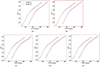 |
Fig. E.1. Orthogonal polynomial fits to one noise realization of case 1 to demonstrate the BIC selection. Panel a: 6th order, Panel b: |

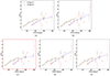 |
Fig. E.2. Orthogonal polynomial fits to one noise realization of case 3 to demonstrate the BIC selection. For the 3rd order, the retrieved time delay and differential dust extinction deviate strongly from the input, which is visible from the different shapes of the fits in the range of the data points of image A and image B. Panel a: 6th order, Panel b: 5th order, Panel c: |

BIC values for the noise realizations shown in Fig. E.1 and Fig. E.2.
All Tables
Results of the time-delay and differential dust extinction retrieval for each investigated S/N and color curve scenario.
All Figures
|
Fig. 1. Exemplary noiseless LSN IIP color curves of two lensing images A and B showing a time shift Δt and a shift in color s due to extinction. |
| In the text | |
|
Fig. 2. u, g, and r light curves of SN2005J observed by the CSP (Anderson et al. 2024) including examples of orthogonal polynomial fits (solid lines) to the u, g and r band light curves. |
| In the text | |
|
Fig. 3. Corner plots of the MCMC chain results and bar plots of selected orders for 100 noise realizations for case 1. The left panels show corner plots of the time shift and differential dust extinction retrieved from 100 noise realizations for case 1. We plot the contours for the 1σ (68%, solid red line) and 2σ (95%, dashed red line) credible intervals for the differential dust extinction AV, B − AV, A and the time delay Δt. The input values in light blue are Δt = 16.3 days and AV, B − AV, A = 0.2 mag. On the right, we show histograms of the selected orthogonal polynomial orders of fitting using the BIC for the corresponding cases on the left. Panel a: Case 1 with one color curve u − g. Panel b: Orders of fitting selected for case 1 with one color curve u − g. Panel c: Case 1 with two color curves u − g and u − r. Panel d: Orders of fitting selected for case 1 with two color curves u − g and u − r. We impose the same order for both color curves. |
| In the text | |
|
Fig. 4. Same as Fig. 3, but for 500 noise realizations for case 2. Panel a: Case 2 with one color curve u − g. Panel b: Orders of fitting selected for case 2 with one color curve u − g. Panel c: Case 2 with two color curves u − g and u − r. Panel d: Orders of fitting selected for case 2 with two color curves u − g and u − r. We impose the same order for both color curves. |
| In the text | |
|
Fig. 5. Same as Fig. 3, but for 500 noise realizations for case 3. Panel a: Case 3 with one color curve u − g. Panel b: Orders of fitting selected for case 3 with one color curve u − g. Panel c: Case 3 with two color curves u − g and u − r. Panel d: Orders of fitting selected for case 3 with two color curves u − g and u − r. We impose the same order for both color curves. |
| In the text | |
|
Fig. 6. Rest-frame u − g color curve and corresponding redshifted r − i color curve created from model spectra. The kink of the rest-frame color curve is slightly weakened by the K-correction. |
| In the text | |
|
Fig. 7. uvw1 − b color curves of SWIFT SNe SN2017eaw (blue) (Szalai et al. 2019) and SN2020jfo (green) (Sollerman et al. 2021). |
| In the text | |
|
Fig. 8. Color curves uvw1 − b (blue) and uvw1* − b (orange) created with the Dessart et al. (2013) model spectra using the SWIFT filters uvw1, b, and the modified uvw1*, where the red tail has been cut. The color curve uvw1* − b still shows a sufficiently strong kink for our time delay method to work. |
| In the text | |
|
Fig. A.1. Corner plot for mock data created with spline fitting, including 100 noise realizations with high S/N. The initial input values shown in light blue are Δt = 16.3 days and AV, B − AV, A = 0.2 mag. |
| In the text | |
|
Fig. A.2. Corner plot for mock data created with spline fitting including 500 noise realizations with low S/N. The initial input values shown in light blue are Δt = 16.3 days and AV, B − AV, A = 0.2 mag. |
| In the text | |
|
Fig. A.3. Histogram of the selected orthogonal polynomial orders of fitting using the BIC for the low S/N mock data created with spline fitting. |
| In the text | |
|
Fig. B.1. Corner plot combining 100 noise realizations of perfect linear mock color curves u − g. Because of the linearity of the mock data, a complete degeneracy is retrieved. |
| In the text | |
|
Fig. C.1. Corner plot of 100 noise realizations of high S/N mock data with Δtsmall = 0.5 days and AV, B − AV, A = 0.2 mag |
| In the text | |
|
Fig. C.2. Corner plot of 100 noise realizations of high S/N mock data with Δtlarge = 50.0 days and AV, B − AV, A = 0.2 mag |
| In the text | |
|
Fig. D.1. Corner plot of 100 noise realizations of low S/N mock data with 35% data loss and with input time delay Δt = 16.3 days for combining u − g and u − r color curves setting RV = 2.0 during MCMC sampling. |
| In the text | |
|
Fig. D.2. Corner plot of 100 noise realizations of low S/N mock data with 35% data loss and with input time delay Δt = 16.3 days for combining u − g and u − r color curves setting RV = 5.0 during MCMC sampling. |
| In the text | |
|
Fig. D.3. Corner plot of 100 noise realizations of low S/N mock data with 35% data loss and with input time delay Δt = 16.3 days for combining u − g and u − r color curves using extinction laws by Gordon et al. (2023) with RV = 3.1 during MCMC sampling. |
| In the text | |
|
Fig. E.1. Orthogonal polynomial fits to one noise realization of case 1 to demonstrate the BIC selection. Panel a: 6th order, Panel b: |
| In the text | |
|
Fig. E.2. Orthogonal polynomial fits to one noise realization of case 3 to demonstrate the BIC selection. For the 3rd order, the retrieved time delay and differential dust extinction deviate strongly from the input, which is visible from the different shapes of the fits in the range of the data points of image A and image B. Panel a: 6th order, Panel b: 5th order, Panel c: |
| In the text | |
Current usage metrics show cumulative count of Article Views (full-text article views including HTML views, PDF and ePub downloads, according to the available data) and Abstracts Views on Vision4Press platform.
Data correspond to usage on the plateform after 2015. The current usage metrics is available 48-96 hours after online publication and is updated daily on week days.
Initial download of the metrics may take a while.