| Issue |
A&A
Volume 698, June 2025
|
|
|---|---|---|
| Article Number | A266 | |
| Number of page(s) | 15 | |
| Section | Cosmology (including clusters of galaxies) | |
| DOI | https://doi.org/10.1051/0004-6361/202553880 | |
| Published online | 20 June 2025 | |
Detection of unresolved strongly lensed supernovae with the 7-Dimensional Telescope
1
Astronomy Research Center, Research Institute of Basic Sciences, Seoul National University, 1 Gwanak-ro, Gwanak-gu, Seoul 08826, Korea
2
Korea Astronomy and Space Science Institute (KASI), 776 Daedeok-daero, Yuseong-gu, Daejeon 34055, Korea
3
KASI Campus, University of Science and Technology, 217 Gajeong-ro, Yuseong-gu, Daejeon 34113, Korea
4
Lawrence Berkeley National Laboratory, 1 Cyclotron Road, Berkeley, CA 94720, USA
5
Department of Physics, University of California Merced, 5200 North Lake Road, Merced, CA 95343, USA
6
Department of Physics & Astronomy, University of California, Los Angeles 430 Portola Plaza, Los Angeles, CA 90095, USA
7
Astronomy Program, Department of Physics and Astronomy, SNU, Seoul, Republic of Korea
8
Department of Physics & Astronomy, University of San Francisco 2130 Fulton Street, San Francisco, CA 94117-1080, USA
9
Physics Division, Lawrence Berkeley National Laboratory 1 Cyclotron Road, Berkeley, CA 94720, USA
⋆ Corresponding authors: This email address is being protected from spambots. You need JavaScript enabled to view it.
, This email address is being protected from spambots. You need JavaScript enabled to view it.
Received:
24
January
2025
Accepted:
24
April
2025
Abstract
Gravitationally lensed supernovae (glSNe) are a powerful tool for exploring the realms of astronomy and cosmology. Time-delay measurements and the lens modeling of glSNe can provide a robust and independent method for constraining the expansion rate of the Universe. The study of the light curves of unresolved glSNe presents a unique opportunity for using small telescopes to investigate these systems. We investigate diverse observational strategies for the initial detection of glSNe using the 7-Dimensional Telescope (7DT). This multitelescope system is composed of twenty 50 cm telescopes. We implement different observing strategies on a subset of 5807 strong-lensing systems and candidates identified within the Dark Energy Camera Legacy Survey (DECaLS), as reported in various publications. Our simulations under ideal observing conditions indicate the maximum expected annual detection rates for various glSN types (type Ia and core-collapse (CC)) using the 7DT target-observing mode in the r band at a depth of 22.04 mag as follows: 7.46 events for type Ia, 2.49 for type Ic, 0.8 for type IIb, 0.52 for type IIL, 0.78 for type IIn, 3.75 for type IIP, and 1.15 for type Ib. Furthermore, in the case of medium-band filter observations (m6000) at a depth of 20.61 in the Wide-field Time-domain Survey (WTS) program, the predicted detection rate for glSNe Ia is 2.53 yr−1. These initially detected systems will be followed-up with observations with more powerful telescopes, and we therefore applied a model-independent approach to forecast the ability of measuring H0 using a Gaussian process from type Ia supernovae (SNe Ia) data and time-delay distance information derived from glSN systems, which include both Ia and CC types. We forecast that the expected detection rate of glSN systems can achieve a precision of 2.7% in estimating the H0.
Key words: gravitational lensing: strong / methods: statistical / telescopes / supernovae: general / cosmology: observations
© The Authors 2025
 Open Access article, published by EDP Sciences, under the terms of the Creative Commons Attribution License (https://creativecommons.org/licenses/by/4.0), which permits unrestricted use, distribution, and reproduction in any medium, provided the original work is properly cited.
This article is published in open access under the Subscribe to Open model. This email address is being protected from spambots. You need JavaScript enabled to view it. to support open access publication.
1. Introduction
The λ cold dark matter (ΛCDM) model serves as the standard framework in cosmology. This model provides explanations for a wide array of current observations, including radiation from the cosmic microwave background (CMB) and baryon acoustic oscillations (BAO) (Schlegel et al. 2009; Planck Collaboration XVI 2014; Planck Collaboration XIII 2016; Planck Collaboration VI 2020; Alam et al. 2021). Despite its successes, the model struggles to resolve differences in the measurements of the current expansion speed of the Universe (Di Valentino et al. 2021). These discrepancies arise when estimates derived from observations of the early Universe (Planck Collaboration VI 2020) are compared with those obtained from local observations, such as type Ia supernovae (SNe Ia) that are calibrated by Cepheid variable stars (Riess et al. 2022).
Gravitationally lensed transients such as quasars (QSOs) and supernovae (SNe) operate as independent cosmological probes capable of constraining the Hubble constant (H0) (Treu et al. 2022, and references therein). This is achieved through a direct estimation of H0 using time-delay measurements in combination with precise lens modeling (Refsdal & Bondi 1964; Refsdal 1964; Oguri 2007; Birrer et al. 2020; Birrer & Treu 2021; Kelly et al. 2023a; Pascale et al. 2025). The abundance of lensed QSOs makes them a consistent and reliable resource for time-delay cosmography. Although hundreds of lensed QSOs have been identified (Lemon et al. 2023), it remains a challenging task to accurately measure their time delays (Liao et al. 2015). This difficulty arises from their stochastic light curves and their variability on year-long timescales, which requires prolonged monitoring with high-resolution telescopes that is both time-consuming and costly (Millon et al. 2020). As a result, only a small fraction of the lensed QSOs have been used for cosmological studies (e.g., Wong et al. 2020; Shajib et al. 2020, 2023). Gravitationally lensed supernovae (glSNe) play a pivotal role in cosmology because they offer several distinct advantages. Their well-defined light curves enable precise measurements of the time delays and H0. In particular, the unique properties of SNe Ia as standard candles allow us to directly measure the intrinsic luminosities when the magnification effects caused by microlensing from stars in the foreground lens galaxy can be mitigated (Foxley-Marrable et al. 2018; Weisenbach et al. 2021). Moreover, Birrer et al. (2022) highlighted that the standardizable brightness of glSNe Ia provides tighter constraints on lens-mass models by effectively addressing the mass-sheet degeneracy (Falco et al. 1985; Schneider & Sluse 2013) and reducing systematic uncertainties in the determination of H0. Additionally, follow-up observations after the glSNe have faded enable detailed studies of the stellar kinematics and host galaxies (Ding et al. 2021; Suyu et al. 2024).
To date, a total of nine SNe have been confirmed to be strongly gravitationally lensed. They are PS1–10afx (Quimby et al. 2014), SN Refsdal (Kelly et al. 2015), SN 2016geu (Goobar et al. 2017), SN Requiem (Rodney et al. 2021), AT 2022riv (Kelly et al. 2022), SN Zwicky (Goobar et al. 2023; Pierel et al. 2023), C22 (Chen et al. 2022), SN H0pe (Frye et al. 2024; Polletta et al. 2023), and SN Encore (Pierel et al. 2024; Dhawan et al. 2024). Each of these SNe is lensed by either a single galaxy or a cluster of galaxies. Observed at a redshift of 1.49, SN Refsdal initially presented four lensed images in 2014, followed by the detection of a fifth image in 2015 (Kelly et al. 2015). Using the time-delay data between these images, Kelly et al. (2023a, b) conducted an analysis that estimated H0 to be  km s−1 Mpc−1. This work demonstrated that gravitational-lensing phenomena can enhance our understanding of cosmology-scale parameters. Recently, SNH0pe was identified as the first gravitational-lensing system discovered with the James Webb Space Telescope (JWST). This system is magnified by the galaxy cluster PLCK–G165.7+67.0 (Frye et al. 2024; Polletta et al. 2023). Pascale et al. (2025) have presented the first measurement of
  km s−1 Mpc−1 from SNH0pe.
Simulation studies indicate that given the limiting magnitude threshold and observing strategy, hundreds of glSNe could be discovered each year with the Rubin Legacy Survey of Space and Time (LSST; see, e.g., Shajib et al. 2024 for a review). Pierel et al. (2021) forecast that the Roman Space Telescope will significantly advance the discovery of glSN systems, which include both type Ia and core-collapse (CC) SNe. Their study demonstrated that various types of glSNe can refine the cosmological parameters, including H0, which provides a strong motivation for focusing observational studies on different types of glSN events. The Roman Space Telescope has an angular resolution of approximately 0.11 arcsec and will be capable of resolving glSN images with significantly smaller separations than the LSST, which has an angular resolution of about 0.5 arcsec. Furthermore, Roman will primarily detect glSNe at higher redshifts, which makes it especially valuable as a high-redshift survey instrument for cosmographic studies that use glSNe (Pierel et al. 2021).
Recently, imaging surveys have identified thousands of new strong lenses and candidates, the majority of which are galaxy-scale lenses, along with a smaller number of group or cluster lenses (e.g., Jacobs et al. 2019; Huang et al. 2020, 2021; Cañameras et al. 2021, 2020; Shu et al. 2022; Stein et al. 2022; Sheu et al. 2023; Storfer et al. 2024; Townsend et al. 2025). The study of these systems is beneficial because the expected time delays from these systems are useful for constraining the H0. We explore the capabilities of the 7-Dimensional Telescope (7DT), which is a multitelescope system comprising up to twenty 0.5-meter wide-field telescopes (Im 2021; Paek et al. 2024; Kim et al. 2024), for the initial detection of glSNe (including both type Ia and CC) under different observing scenarios among this newly identified sample of strong-lens and candidate systems. The 7DT has an inimitable combination of a wide field of view, flexible multitelescope operations, and a transient classification using medium-band filters. These capabilities enable the 7DT to discover glSNe. It is worth noting that due to the limited angular resolution of the telescopes, numerous gLSNe remain unresolved (Goldstein et al. 2019). As mentioned by Bag et al. (2024), unresolved glSNe exhibit shorter time delays, which increase the total brightness within a seeing disk. This enhanced brightness offers a distinct advantage for small-telescope arrays with a limited sensitivity, thereby enabling the early detection of glSNe. Moreover, the magnification estimates derived from glSN systems, particularly for glSNe Ia, may offer valuable constraints for modeling the lensing-mass distributions in observed systems. However, the shorter time delay also presents a disadvantage because it reduces the precision of the time-delay measurements, which affects precise estimates of H0. We selected a sample of lensed galaxies and candidates (Huang et al. 2020, 2021; Storfer et al. 2024) from the footprint of the DESI Legacy Imaging Surveys (Dey et al. 2019). Following the approach presented by Sheu et al. (2023) for generating synthetic glSN light curves and estimating the expected rate of these systems, we demonstrate the potential of 7DT for the initial detection of glSNe. Following the initial detection, we propose conducting follow-up observations with powerful telescopes to constrain H0 using both types of glSNe, that is, type Ia and CC SNe. We use a model-independent approach (Liao et al. 2019, 2020) (i.e., we assume no specific cosmological model) to determine H0 by anchoring type Ia SNe from the Pantheon dataset (Scolnic et al. 2018) with detected strong-lensed systems.
The structure of this paper is organized as follows: Section 2 details the observation capabilities of the 7DT facility. In Section 3 we describe the selection of the target fields for glSN observations and focus on the spatial distribution of lenses and candidates that were identified from the DESI imaging survey. Based on the results of the glSN simulation, we propose various observing strategies with the 7DT. With respect to the detection rate of glSNe based on the 7DT observing scenario, we provide an estimate of H0 in Section 4. In the concluding Section 5, we present a summary of the key findings and discuss the implications of our research.
2. Observation capabilities of the 7-Dimensional Telescope
The 7DT is a multiple telescope system (Im 2021; Paek et al. 2024; Kim et al. 2024). This system encompasses twenty 0.5-meter telescopes that are positioned at the El Sauce Observatory within the Rio Hurtado Valley in Chile. The typical seeing at this site is about 1.5 arcsec. The angular resolution of the 7DT is primarily constrained by the seeing conditions at the site. Fifteen of the 20 planned telescopes are currently positioned. Each single telescope in this multiple telescope system has a field of view (FOV) of 1.27 deg2 (0.92 deg × 1.38 deg).
Each telescope in the 7DT system is equipped with Sloan g-, r-, and i-band filters. Additionally, the entire system includes one u-band filter and three z-band filters. The system also includes 40 medium-band filters characterized by a bandwidth of 25 nm, covering a spectral range from 375 nm to 900 nm with a gap of 12.5 nm between them. At present, 20 medium-band filters are in operation. Their central wavelengths range from 400 nm to 887.5 nm, with gaps of 25 nm between them (Figure 1). The 7DT achieves a remarkable combination of features: (i) A flexible operation with multiple telescopes, (ii) a wide field of view, and (iii) a transient classification using medium-band filters. These attributes make it an outstanding discovery instrument for glSNe.
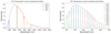 |
Fig. 1. 7DT transmission curves for broad- and medium-band filters. |
The 7DT encompasses a variety of operational modes (Kim et al. 2024). These modes include the (1) spec mode: the 7DT employs various medium-band filters in a single pointing to enable spectral mapping of the sky. (2) The search mode: The 20 telescopes of the 7DT observe various patches of the sky using broadband filters. In this mode, the 7DT can survey a vast area of the sky. The total FOV is approximately (20 × 1.27) ∼ 25 deg2. (3) The deep-observing mode can operate in several configurations. To streamline operations, we recommend limiting configurations such as 20, 10, 4, or 2 telescopes per pointing. When all 20 telescopes are pointed at the same area using a single filter, the system achieves its highest sensitivity, which is equivalent to the light-collecting capability of a 2.3-meter diameter telescope.
In the following, we introduce two primary observational strategies implemented with the 7DT (Kim et al. 2024):
-
The 7-Dimensional Sky Survey (7DS) is a comprehensive wide-field time-series survey that employs a multi-object spectroscopy approach with medium-band filters. The survey observations conducted by the 7DS will include the Reference Image Survey (RIS), the Wide-field Time-domain Survey (WTS), and the Intensive Monitoring Survey (IMS).
The RIS encompasses an area of 20 000 deg2 of the southern sky, excluding the Galactic plane. Observations are conducted with a uniform cadence and an exposure time of 100 seconds per tile. Each tile is observed three times per visit, totaling a 5-minute exposure time. The total allocated observation time for this survey is 50 000 minutes. The RIS begins in the first year of the 7DS observation. This area is observed once to generate reference images that are used for identifying transient events through a difference-image analysis (DIA). The DIA accomplishes this by subtracting the reference image from each individual image (e.g., Bramich et al. 2013).
The WTS monitors approximately 1620 deg2 of the southern sky with a 14-day cadence over a planned 5-year observational period. The field selection for this survey is currently under discussion, with particular emphasis on regions possessing complementary data, especially those with existing near-infrared photometry.
The IMS covers the AKARI Deep Field South (ADF-S) (Matsuura et al. 2011; Murakami et al. 2007), a 12 deg2 region near the south ecliptic pole, with daily observations. The survey allocates a total of 20 000 minutes of observation time per year.
-
The target of opportunity observation (ToO) approach is used by the 7DT to streamline the detection of various transient phenomena, including the electromagnetic (EM) counterparts of gravitational-wave (GW) events. The same configuration as RIS, specifically, using 5-minute exposures with medium-band filters, is applied to this program.
3. Exploring observation strategies for strongly lensed supernovae with 7DT
In this section, we introduce observation strategies for glSNe that were developed based on the analysis of synthetic glSN light curves. This development uses information from confirmed strong gravitational lenses and candidate lenses identified in the Dark Energy Spectroscopic Instrument (DESI) Legacy Imaging Surveys (Huang et al. 2020, 2021; Storfer et al. 2024).
3.1. Identifying target fields for glSN observation
Recently, Sheu et al. (2023) used an archive comprising 5807 strong lenses and potential candidates identified through the Dark Energy Camera Legacy Survey (DECaLS) to develop a specialized pipeline to search for the glSNe. DECaLS is a key project for the DESI Legacy Imaging Surveys and operates using the Dark Energy Camera mounted on the 4-meter Blanco telescope situated at the Cerro Tololo Inter-American Observatory. This wide-field survey spans an area of the sky of 9000 deg2 that encompasses both the north Galactic cap (NGC; declination <32 deg) and the south Galactic cap in the g, r, and z bands. The lens candidates examined in their search originate from a variety of publications and search efforts. To assess the likelihood that a candidate represents a strong-lens system, the criteria used in this paper are similar to those described by Huang et al. (2021). We selected a sample of lens systems and candidates for a targeted observation from Huang et al. (2020, 2021), Storfer et al. (2024)1, located at declinations below 30°. We used the spectroscopic or photometric redshifts of these lens systems and candidates to construct the lens redshift distribution. Then, we adopted the method for simulating the redshift of glSNe as outlined by Sheu et al. (2023). We obtained the source redshift distribution by multiplying the lens redshift distribution by a truncated normal distribution N(2,0.5), with a lower bound at one.
Furthermore, following the approach described by Sheu et al. (2023), we estimated the star formation rate (SFR) across different redshifts by fitting a polynomial function to the SFR data provided by Bell et al. (2007), Smit et al. (2012), and Sobral et al. (2013). We calculated the annual CC SNe rate using
![Mathematical equation: $$ R_{\mathrm {CC}} = kcc\frac {{\mathrm {SFR}}}{1+z_{\mathrm {s}}} [{\mathrm {yr}}^{-1}], $$](/articles/aa/full_html/2025/06/aa53880-25/aa53880-25-eq3.gif) (1)
(1)
where the number of CC SNe is kcc = 0.0068M−1 (Shu et al. 2018).
We estimated the annual rate of SNe Ia through the equation
![Mathematical equation: $$ R_{\mathrm {Ia}} = 0.00084M^{-1}_\odot \frac {\int ^{t(z_{\mathrm {s}})}_{0.1} {\mathrm {SFR}}(t(z_{\mathrm {s}})-t_{\mathrm {D}})f_{\mathrm {D}}(t_{\mathrm {D}})\,{\mathrm {d}}t_{\mathrm {D}}}{(1+z_{\mathrm {s}}) \int _{0.1}^{t(z = 0)}f_{\mathrm {D}}(t_{\mathrm {D}})\,{\mathrm {d}}t_{\mathrm {D}}} [{\mathrm {yr}}^{-1}], $$](/articles/aa/full_html/2025/06/aa53880-25/aa53880-25-eq4.gif) (2)
(2)
where tD represents the delay time and follows a distribution  (Shu et al. 2018). We used the formula from Equation (2) by Sheu et al. (2023) to calculate the star formation history of the lensed sources (SFR(t(zs)−tD)). We limited our selection to systems with a glSNe redshift below 0.7 to ensure that they are bright enough to be detected within the sensitivity limits of the telescope. We conducted the simulation 100 times to ensure statistically robust and realistic results. Figure 2 illustrates the strong-lensing plausibility of these systems. Figure 3 presents the redshift distributions of the selected lens systems and candidates, the simulated source galaxies, and the distribution of the ratios of the lens redshift to source redshift.
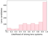 |
Fig. 2. Likelihood of lens candidates. |
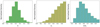 |
Fig. 3. Redshift distribution for selected lens galaxies and candidates zl, simulated source galaxies zs, and the ratio zl/zs. |
We generated a sky tiling for 7DT to coordinate the glSN observations. To improve the transient identification, we incorporated overlaps between the tiles (Figure 4). Additionally, Figure 4 displays the spatial locations of the selected lens systems and candidates. About 1225 lens systems and candidates are distributed across approximately 1125 7DT fields.
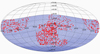 |
Fig. 4. 7DT sky footprint (blue tile patterns) and location of selected lens galaxies and candidates (red dots). The approximate number of targeted 7DT fields covering the systems is 1125 tiles. |
In the following sections, we explore the process of creating synthetic light curves for every system in our simulation. We also investigate the effect of unresolved glSNe images on the light curves. Regarding the output result, we determine the monitoring duration and cadence to give a glSN observing strategy with 7DT.
3.2. Generating glSN light curves
We employed the SNCosmo software (Barbary et al. 2024) to simulate the SN light curves. We used the SALT3 model to generate type Ia SN light curves. The critical parameters for this model include the redshift, flux normalization (x0), color (c), and stretch (x1) (Kenworthy et al. 2021). We adopted the same parameter settings as were used by Arendse et al. (2024)2. Specifically, x1 was drawn from a skew-normal distribution, x1∼Ns(a=−8.24,μ = 1.23,σ = 1.67), c followed a skew-normal distribution, c∼Ns(a = 2.48,μ=−0.089,σ = 0.12), and the absolute B-band magnitude (MB) was sampled from a normal distribution, MB∼N(μ=−19.43,σ = 0.12).
The SNCosmo package also provides a variety of CC models for SNe. This allowed us to choose different models for each SN type. We employed various models for our analyses, including Nugent-SN2P (type IIP) (Gilliland et al. 1999), SNANA-2004GQ (type Ic)3, V19-2008AQ-CORR (type IIb)4, S11-2005HL (type Ib) (Sako et al. 2011), Nugent-SN2L (type IIL) (Gilliland et al. 1999), and Nugent-SN2N (type IIn) (Gilliland et al. 1999). These models are characterized by parameters such as the redshift (z), amplitude, and the time of peak brightness in the B band (t0). We used the distribution of MB and the occurrence rates of various types of CC SNe from Table 1 of Sheu et al. (2023). We acknowledge that a more realistic approach would involve randomly sampling from multiple CC models for SNe within each subtype. This is a limitation of the current study.
For the simulated light curves of glSNe, we considered the effects of dust extinction originating from both the host galaxy and the Milky Way, following the dust-extinction model proposed by Fitzpatrick (1999). For the host galaxy, we assumed a dust extinction characterized by a color excess E(B−V)host≤0.2 and a selective-to-total extinction ratio RV in the range [1.63, 3.85]. For the Milky Way extinction, we adopted a standard extinction ratio of RV = 3.1, with E(B−V)MW values derived using the dustmaps package (Green 2018), based on the dust-reddening map provided by Chiang (2023).
3.3. Unresolved glSN light curve
Strong gravitational lensing can produce images with varying magnified fluxes and time delays. However, because of the angular resolution limitations of ground-based telescopes, which are influenced by atmospheric conditions (seeing), these images may overlap. As a result, they can appear to be blended or are indistinguishable. When the image separation becomes too small, a unified light curve is recorded (Bag et al. 2021; Denissenya et al. 2022). As outlined by Goldstein et al. (2019), it is anticipated that more than half of the glSNe detected by the LSST will have an angular resolution lower than 1″. A significant fraction of these systems will exhibit separations below 0.5″ (Bag et al. 2024). Because the typical seeing for the LSST is 0.7″ in the r band (LSST Science Collaboration 2009), a considerable portion of the strong-lensing systems will likely be unresolved by this wide-field survey. Bag et al. (2024) reported that unresolved systems have shorter time delays than resolved systems. Their findings indicated that for unresolved systems in the LSST, the median time delay is 2.03 days. Only about 10% of these systems have time delays longer than 10 days. The findings were presented in Figure 11 of Sagués Carracedo et al. (2024) for the Zwicky Transient Facility (ZTF), with a spatial resolution of 2″ for this telescope. They revealed that most events have angular separations below 1″. Furthermore, the majority of these events exhibit time delays shorter than 10 days, with a median delay of approximately 5 days.
Following the method outlined by Sheu et al. (2023), we assumed that each lensing system produces either two or four lensed images with probabilities of 0.7 and 0.3, respectively. This is consistent with the results from Oguri & Marshall (2010). For each system, Sheu et al. (2023) sampled the magnifications from a log-normal distribution with a mean of 1.5 and a standard deviation of 0.35, resulting in an expected magnification of 4.765. They also sampled the time delays between the lensed images for each system from a normal distribution, N(36,4) days, as described in Craig et al. (2024). Inspired by the findings of Bag et al. (2024), Sagués Carracedo et al. (2024), we refined the time-delay and magnification distributions in our simulation. We selected the magnification as a log-normal distribution with a mean = 1.07 and a dstandard deviation = 0.465. We sample the time-delay distribution from an exponential distribution5 with a mean of 6.83. The mean and standard deviation were selected based on the values provided in Table 3 of Sagués Carracedo et al. (2024)6. We conducted our simulation in two steps. First, we assumed that approximately 50% of the images in a system are completely unresolved. In the second step, we ran the simulation under the assumption that 90% of the images in a system are completely unresolved.
It is important to note that for simplicity, we ignored the microlensig effect due to stars in the lens galaxy or in the foreground lens galaxy. Microlensing can affect the observed brightness of glSNe and either magnify or suppress their brightness. A brightness suppression occurs more frequently than a magnification (Goldstein et al. 2018; Arendse et al. 2024). Microlensing also impacts unresolved sources differently from resolved ones. For unresolved sources, the observed flux is the sum of the individual fluxes from multiple images, each of which may be intrinsically fainter than those of resolved sources. Although microlensing affects each individual image differently, the summed flux of the unresolved images is often still higher than the detection threshold, which effectively reduces the overall impact of microlensing on the peak brightness measurements. As a result, incorporating microlensing into analyses would likely increase the predicted ratio of unresolved to resolved SN detections (Bag et al. 2024). Furthermore, microlensing introduces substantial uncertainties in time-delay measurements (Goldstein et al. 2018), particularly for glSNe with inherently short delays (e.g., Goobar et al. 2017; Huber et al. 2019). While we acknowledge the importance of microlensing, we explicitly state that modeling its effects is beyond the scope of this paper and constitutes a caveat of our analysis. In the next subsection, we present various observing strategies with 7DT and calculate the annual detection rates for each strategy.
3.4. Observing scenarios
3.4.1. 7-Dimensional Sky Survey (7DS)
The 7DS conducts the WTS as a core program in spec mode for a 5-year observation period. The advantage of observing in different medium-band filters is the classification of transients. The exposure time for this program is set to 300 s. The 5σ depth of the 7DT for the medium-band filters at 300 s is listed in Table 1. The depths given for various exposure times are simulated values based on ideal conditions, including 1.5″ seeing, gray moon phase, and marginal target altitude. To optimally determine the cadence for glSN observations, we calculated the control time of mock light curves in our simulations. The control time is determined as described below.
-
For systems with resolved images, we consider the first bright image in the system. The control time is defined as the width of the light curve of this image at a magnitude equal to the observing depth of the telescope.
-
For systems with unresolved images, the control time is determined as the width of the combined light curve at a magnitude equal to the observing depth of the telescope.
Because WTS conducts a relatively shallow survey, only the brightest objects can reach our detection limits. Considering the intrinsic brightness of different types of SNe, our simulations indicate that SNe Ia (which are intrinsically much brighter than other SN types) are most likely to be observed. While some highly magnified or intrinsically bright CC SNe could still be detectable, their expected occurrence is lower.
5σ depth magnitudes in various filters for the 7-DT in 300 s exposure times.
The control-time distribution of glSNe Ia, assuming that 90% of the systems have completely unresolved images, across various medium-band filters is presented in Figure A.1. These findings highlight that as discussed in Section 2, the 14-day cadence proposed for this program is well suited for glSN Ia observations. We estimated the annual detection rate of glSN Ia events based on the depth of observations conducted with the 7DS-WTS program in spec mode. For this estimation, we used the formation rate formulation of glSNe Ia presented by Sect. 3.1 as a first-order approximation. A system is considered detectable with 7DT when the peak brightness of at least one image within the system exceeds the observation depth. Figure 5 illustrates the detection rates of glSNe Ia, assuming that 90% of the systems have completely unresolved images. We expect to observe up to 2.53 events per year for systems with a redshift <0.6 as part of the 7DS-WTS program. However, based on simulation results, systems with a redshift in the range 0.6<zs<0.7 are not detectable by the WTS program. It is important to highlight that the expected detection rates depend on the observing conditions, such as the moon phase and seeing, and can vary accordingly.
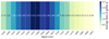 |
Fig. 5. Average detection rate of glSNe Ia for different 7DT medium-band filters and source redshifts zs≤0.6, assuming 90% of systems are unresolved. |
3.4.2. 7DT target program for glSNe observations
We recommend implementing the glSNe observations as a program designed to target specific regions of the sky. This program can operate in search mode or deep mode as a targeted survey using a broadband filter. The glSNe exhibit redder colors, indicating that observations in the near-infrared are more suitable. However, because the sensitivity of the 7DT is lower in the i and z bands, we focused on a detection of glSNe in the r band. For this program, we recommend a monitoring duration from 7 to 14 days. This monitoring cadence is derived from the analysis of the control-time distributions generated from mock light curves in the r-band filter at depths of 21.02 magnitudes (with an exposure time of 60 seconds) and 22.04 magnitudes (with an exposure time of 360 seconds). Figure 6 (upper panel for glSNe Ia) and Figures B.1 and B.2 (for glSNe CC) illustrate the control time distributions corresponding to 50% and 90% of systems with completely unresolved images.
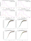 |
Fig. 6. Upper panels: Control time distribution of glSNe Ia at different observing depths for source redshifts zs≤0.6 and zs>0.6, considering (1) 50% and (2) 90% of systems are unresolved. Black vertical lines indicate the median control times. Lower panel: Annual detection rate of glSNe Ia as a function of lens redshift calculated from 100 simulation realizations (individual realizations shown by colored lines). We present results at different observational depths, accounting for (1) 50% and (2) 90% of systems being unresolved. |
This targeted survey is categorized into two groups based on the depth of the observation and required exposure times to achieve certain magnitudes: (1) the shallow observation, which enables us to reach a magnitude of ≤21.02, and (2) the deep observation, designed to seek deeper insight with a magnitude of ≤22.04 mag.
-
In the shallow observation, each telescope in the 7-DT array can achieve a magnitude of 21.02 with a one-minute exposure. With an observing duration of 7 hours per night and accounting for approximately 10% overhead (including 10-second slewing, 100-second auto focus, 5-second image readout, and 5−10 seconds for filter changes and focusing), we can cover all target tiles (∼1125) within 2 hours. By observing in a single filter, we can effectively identify transients by employing reference images obtained from the RIS.
-
In deep observations, various configurations can be applied, as discussed in Section 2. A single 7DT telescope can achieve a 22.04 magnitude with a 6-minute exposure time in the r band, and we therefore recommend using two telescopes per pointing, with each tile observed for 3 minutes. However, it is important to note that increasing the number of telescopes per tile will lead to higher overhead times due to the need for telescope adjustments. In this case, for 7-hour observations per night, all target tiles can cover a depth of 22.04 mag. We conduct observations using at least one single filter (r band).
It should be noted that the expected exposure time can vary depending on conditions such as the moon phase and seeing. The suggested exposure times, that is, 1 minute for a depth of 21.02 and 6 minutes for a depth of 22.04, are based on simulations under ideal conditions. When observing under less favorable conditions, longer exposure times are required. Consequently, to cover all target tiles in real observations, additional observing time may be necessary.
When a transient is detected, follow-up observations using different medium-band filters should be performed in the same field to verify the characteristics of the transient.
We provide a rough estimation of the glSN detection rate in the r band. For this estimation, we adopted the formation rate formulation of glSNe Ia and CC outlined in Sect. 3.1 as a first-order approximation. Figure 6 (lower panel for glSNe Ia) and Figures C.1 and C.2 (for glSNe CC) display the detection rates at depths of 21.02 and 22.04 magnitudes, representing 50% and 90% of systems with completely unresolved images.
It is important to emphasize that the LSST provides significantly more advanced observational capabilities than the single r-band 7DT target program for glSN observations. However, because not everyone has access to the LSST and many astronomers rely on smaller telescopes, our motivation for this observing strategy is to demonstrate that even modest facilities can still make meaningful contributions to cosmology.
3.5. Integrating 7DT with LSST for glSN observation
The LSST7 is an 8.4-meter ground-based telescope located on Cerro Pachón in north-central Chile. The LSST is designed to conduct a multiband imaging survey, covering approximately 20 000 square degrees of the sky with a 9.6 square-degree field of view (LSST Science Collaboration 2009). Several studies (Goldstein et al. 2019; Arendse et al. 2024; Rydberg et al. 2020; Wojtak et al. 2019) have estimated that LSST could detect on the order of tens to hundreds of glSNe annually. The expected number of these detections depends on the observing strategy, which varies with factors such as cadence, depth, filter configuration, and sky coverage. The LSST observing scenario is expected to implement rolling-cadence strategies approximately 1.5 years after the survey begins. In this approach, the LSST Wide Fast Deep (WFD) footprint is divided into multiple regions that cycle between a high and low observational cadence across survey years. The rolling cadence results in a nonuniform distribution of visits across seasons. In some seasons, certain regions of the WFD footprint receive more than the typical number of visits (high cadence), while in other seasons, the same regions receive fewer than average (low cadence).
During low-cadence seasons, each field typically receives around 25 visits. The season length remains approximately the same in the low- and high-cadence seasons, and it typically spans about 180 days8.
Huber et al. (2019) and Arendse et al. (2024) investigated the impact of rolling-cadence strategies on the number of glSN detections with the LSST.
As shown in Figure 4, the distribution of glSN systems and candidates spans both high- and low-cadence regions within the WFD footprint of LSST. We expect the 7DT strategy to have a higher impact when it targets glSNe fields located in low-cadence regions during the rolling-cadence phase of LSST, although we did not simulate this observing strategy in this paper. The 7DT observes these target fields with broadband filters. When a transient candidate is detected, targeted follow-up observations with a set of medium-band filters are performed in the same field to verify and characterize the transient in detail. This allows the 7DT to provide higher-cadence monitoring in these undersampled areas, enabling earlier detections and improved transient classification through its dedicated medium-band filter set.
4. Cosmology: H0 constraint
In this section, we apply a model-independent method, as presented by Liao et al. (2019, 2020), Li et al. (2024), to constrain H0. This is achieved through anchoring the relative distances of SNe Ia from the Pantheon dataset (Scolnic et al. 2018) with time-delay distance measurements of glSNe. By combining a large statistical sample of type Ia SNe, which are insensitive in this approach to H0, and with a smaller sample of strongly lensed systems that are sensitive to H0, we can estimate H0 without relying on any specific cosmological model (Liao et al. 2019). These glSNe are anticipated to be initially detected with the 7DT and subsequently to be followed-up with high-powered telescopes.
The idea is to forecast the ability of constraining H0 by generating a mock time-delay distance dataset alongside a mock SNe Ia standard candle dataset. We then use Gaussian process (GP) regression to generate realizations of H0DL from the SNe Ia standard candle dataset, which are then anchored by the time-delay distance dataset. This works by evaluating the GP reconstructions of H0DL at the mock strong-lens redshifts for each strong lens system, then turning H0DL into H0DΔt. With a value of H0, we can then compare the model time-delay distances to the mock data time-delay distances (evaluate as a likelihood) for each realization of the GP reconstruction. The posterior on H0 is then just marginalizing over the GP realizations. These model-independent constraints are important because in these high-precision regimes, the assumption of a background cosmological model can bias the inference of the parameters (Shafieloo et al. 2020; Keeley et al. 2020).
We used GP regression9 on the Pantheon SN Ia dataset (Brout et al. 2022; Scolnic et al. 2018). We used this method to generate 1000 reconstructions of the unanchored luminosity distance (H0- independent quantity denoted as H0DL) from the SNe Ia data (Figure 7). Then, we calculated the unanchored angular diameter distance, represented by (H0DA), using the formula  (Hogg 1999). For each system identified in Section 3, we computed 1000 H0DA at the lens and source redshifts, denoted as H0Dl and H0Ds, respectively. Subsequently, we determined the time-delay distances (DΔt) for each system in our gravitational-lensing simulation. For every identified system, we calculated 1000 values of H0DΔt using the equation (Refsdal 1964; Schneider et al. 1992; Suyu et al. 2010)
 (3)
(3)
where l and s represent the lens and the source, respectively, and Dls represents the distance between the lens and the source (Weinberg 1972). Furthermore, j is the index of the realization of the GP reconstruction, and i is the index of each of the N mock strong lens for the different cases.
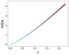 |
Fig. 7. Reconstruction of the H0DL(z) function using GP reconstructions from SNe Ia dataset. |
In the next step, we calculated the likelihood for glSN systems as follows Li et al. (2024) for each realization of the GP reconstruction:
 (4)
(4)
 represents the mock time-delay distance data. These mock data were calculated by taking a flat ΛCDM model with H0 = 70 km/s/Mpc and Ωm = 0.3 and evaluating time-delay distances at redshifts sampled from the procedure we defined in the previous sections. Then, we added 10% noise to these mock time-delay distances, which we estimated to be a reasonable uncertainty associated with the time-delay distances (
 ). We varied the value of H0 in the range [60,80] km/s/Mpc with 121 steps. Finally, we calculated the posterior for H0 by marginalizing over the realizations of H0DL GP reconstructions,
 (5)
(5)
Table 2 presents the best-estimate values of H0 for the expected number of glSN systems, including (1) 7 glSNe Ia, (2) 7 glSNe CC, and (3) the combined sample of glSNe Ia and CC detected through the 7DT deep-target program. It also includes the H0 estimate for two glSNe Ia detected through the 7DS-WTS program.
Best fit values for H0 with 1σ uncertainty at 10% precision in time-delay distance measurements of glSNe.
5. Conclusions
Because the angular resolution of telescopes is limited, a significant portion of glSN systems remains unresolved. As demonstrated by Bag et al. (2024), unresolved systems have shorter time delays than resolved systems. The light curves of unresolved systems are the result of the combined contributions from the individual images of the system. These shorter time delays lead to an increased brightness in the summed light curve, which is advantageous for arrays of small telescopes with low limiting magnitudes. This enables the initial detection of glSNe. However, shorter time delays pose a disadvantage for precise time-delay measurements, thereby impacting the precise estimation of H0. We examined the capability of the 7DT of discovering glSNe under different observing strategies. We used a catalog of strong-lens systems and candidates observed by the DESI Legacy Imaging Surveys (Dey et al. 2019). By using the lens redshift distribution provided in this catalog, along with the formula presented by Shu et al. (2018), Sheu et al. (2023), we conducted simulations to generate various characteristics of lensed systems, including the source redshifts, the number of lensed images, the magnifications for lensed systems, the time delay between images, and the rates of type Ia and CC SNe. Subsequently, we created synthetic light curves for each of the simulated SNe, taking into account an effect of dust from the host galaxy and the Milky Way on these curves. As mentioned by Goldstein et al. (2019), the majority of lensed systems remain unresolved due to the resolution limitations of telescopes. This factor impacts the light curves. To address this, we executed our code twice: initially, under the assumption that the generated images of 50% of the systems are unresolved, and subsequently, assuming that 90% are unresolved.
Based on the simulation outcomes, we anticipate that up to 2 glSNe Ia can be detected with the 7DS-WTS program and up to 7 glSNe Ia and 7 CC events under the 7DT target program. We then assumed that the glSNe initially detected by the 7DT will be followed-up with more powerful telescopes. Furthermore, we proposed a collaborative observing strategy that combines the capabilities of the 7DT and LSST for the glSNe observation. In the next step, we performed a model-independent analysis, free from any assumption about cosmological models, to constrain the H0 using GP regression by anchoring the SNe Ia from the Pantheon dataset with time-delay distances from detected glSNe of type Ia and CC. Our model-independent results yield H0 = 71.4±5.1 km/s/Mpc for two glSNe Ia detected with the 7DS-WTS program, and H0 = 70.03±1.9 km/s/Mpc for the seven glSNe Ia and 7 glSNe CC detected under the deep-targeting scenario proposed for the 7DT observing program.
Acknowledgments
We thank Hyeonho Choi for providing information regarding the 7DT overhead time. E.K., A.S. and H.M.L. are supported by the National Research Foundation of Korea 2021M3F7A1082056. GSHP and MI acknowledge the support from the National Research Foundation of Korea (NRF) grant, No. 2021M3F7A1084525, funded by the Korea government (MSIT).
We selected this distribution based on Fig. 3 of Bag et al. (2024) and the time-delay histogram in Fig. 11 of Sagués Carracedo et al. (2024).
We convert the magnification value to a logarithmic scale.
References
- Alam, S., de Mattia, A., Tamone, A., et al. 2021, MNRAS, 504, 4667 [NASA ADS] [CrossRef] [Google Scholar]
- Arendse, N., Dhawan, S., Sagués Carracedo, A., et al. 2024, MNRAS, 531, 3509 [NASA ADS] [CrossRef] [Google Scholar]
- Bag, S., Kim, A. G., Linder, E. V., & Shafieloo, A. 2021, ApJ, 910, 65 [NASA ADS] [CrossRef] [Google Scholar]
- Bag, S., Huber, S., Suyu, S. H., et al. 2024, A&A, 691, A100 [NASA ADS] [CrossRef] [EDP Sciences] [Google Scholar]
- Barbary, K., Bailey, S., Barentsen, G., et al. 2024, https://zenodo.org/records/10602402 [Google Scholar]
- Bell, E. F., Zheng, X. Z., Papovich, C., et al. 2007, ApJ, 663, 834 [Google Scholar]
- Birrer, S., & Treu, T. 2021, A&A, 649, A61 [NASA ADS] [CrossRef] [EDP Sciences] [Google Scholar]
- Birrer, S., Shajib, A. J., Galan, A., et al. 2020, A&A, 643, A165 [NASA ADS] [CrossRef] [EDP Sciences] [Google Scholar]
- Birrer, S., Dhawan, S., & Shajib, A. J. 2022, ApJ, 924, 2 [NASA ADS] [CrossRef] [Google Scholar]
- Bramich, D. M., Horne, K., Albrow, M. D., et al. 2013, MNRAS, 428, 2275 [NASA ADS] [CrossRef] [Google Scholar]
- Brout, D., Scolnic, D., Popovic, B., et al. 2022, ApJ, 938, 110 [NASA ADS] [CrossRef] [Google Scholar]
- Cañameras, R., Schuldt, S., Suyu, S. H., et al. 2020, A&A, 644, A163 [Google Scholar]
- Cañameras, R., Schuldt, S., Shu, Y., et al. 2021, A&A, 653, L6 [NASA ADS] [CrossRef] [EDP Sciences] [Google Scholar]
- Chen, W., Kelly, P. L., Oguri, M., et al. 2022, Nature, 611, 256 [NASA ADS] [CrossRef] [Google Scholar]
- Chiang, Y. -K. 2023, ApJ, 958, 118 [NASA ADS] [CrossRef] [Google Scholar]
- Craig, P., O’Connor, K., Chakrabarti, S., et al. 2024, MNRAS, 534, 1077 [NASA ADS] [CrossRef] [Google Scholar]
- Denissenya, M., Bag, S., Kim, A. G., Linder, E. V., & Shafieloo, A. 2022, MNRAS, 511, 1210 [NASA ADS] [CrossRef] [Google Scholar]
- Dey, A., Schlegel, D. J., Lang, D., et al. 2019, AJ, 157, 168 [Google Scholar]
- Dhawan, S., Pierel, J. D. R., Gu, M., et al. 2024, MNRAS, 535, 2939 [Google Scholar]
- Ding, X., Liao, K., Birrer, S., et al. 2021, MNRAS, 504, 5621 [NASA ADS] [CrossRef] [Google Scholar]
- Di Valentino, E., Mena, O., Pan, S., et al. 2021, CQG, 38, 153001 [NASA ADS] [CrossRef] [Google Scholar]
- Falco, E. E., Gorenstein, M. V., & Shapiro, I. I. 1985, ApJ, 289, L1 [Google Scholar]
- Fitzpatrick, E. L. 1999, PASP, 111, 63 [Google Scholar]
- Foxley-Marrable, M., Collett, T. E., Vernardos, G., Goldstein, D. A., & Bacon, D. 2018, MNRAS, 478, 5081 [NASA ADS] [CrossRef] [Google Scholar]
- Frye, B. L., Pascale, M., Pierel, J., et al. 2024, ApJ, 961, 171 [NASA ADS] [CrossRef] [Google Scholar]
- Gilliland, R. L., Nugent, P. E., & Phillips, M. M. 1999, ApJ, 521, 30 [NASA ADS] [CrossRef] [Google Scholar]
- Goldstein, D. A., Nugent, P. E., Kasen, D. N., & Collett, T. E. 2018, ApJ, 855, 22 [NASA ADS] [CrossRef] [Google Scholar]
- Goldstein, D. A., Nugent, P. E., & Goobar, A. 2019, ApJS, 243, 6 [NASA ADS] [CrossRef] [Google Scholar]
- Goobar, A., Amanullah, R., Kulkarni, S. R., et al. 2017, Science, 356, 291 [Google Scholar]
- Goobar, A., Johansson, J., Schulze, S., et al. 2023, Nat. Astron., 7, 1098 [NASA ADS] [CrossRef] [Google Scholar]
- Green, G. 2018, J. Open Source Softw., 3, 695 [NASA ADS] [CrossRef] [Google Scholar]
- Hogg, D. W. 1999, ArXiv e-prints [arXiv:astro-ph/9905116] [Google Scholar]
- Huang, X., Storfer, C., Ravi, V., et al. 2020, ApJ, 894, 78 [NASA ADS] [CrossRef] [Google Scholar]
- Huang, X., Storfer, C., Gu, A., et al. 2021, ApJ, 909, 27 [NASA ADS] [CrossRef] [Google Scholar]
- Huber, S., Suyu, S. H., Noebauer, U. M., et al. 2019, A&A, 631, A161 [NASA ADS] [CrossRef] [EDP Sciences] [Google Scholar]
- Im, M. 2021, 43rd COSPAR Scientific Assembly. Held 28 January – 4 February, 43, 1537 [Google Scholar]
- Jacobs, C., Collett, T., Glazebrook, K., et al. 2019, ApJS, 243, 17 [Google Scholar]
- Keeley, R. E., Shafieloo, A., L’Huillier, B., & Linder, E. V. 2020, MNRAS, 491, 3983 [Google Scholar]
- Kelly, P. L., Rodney, S. A., Treu, T., et al. 2015, Science, 347, 1123 [Google Scholar]
- Kelly, P., Zitrin, A., Oguri, M., et al. 2022, Transient Name Server Discovery Report, 2022-2356 1 [Google Scholar]
- Kelly, P. L., Rodney, S., Treu, T., et al. 2023a, Science, 380, abh1322 [NASA ADS] [CrossRef] [Google Scholar]
- Kelly, P. L., Rodney, S., Treu, T., et al. 2023b, ApJ, 948, 93 [NASA ADS] [CrossRef] [Google Scholar]
- Kenworthy, W. D., Jones, D. O., Dai, M., et al. 2021, ApJ, 923, 265 [NASA ADS] [CrossRef] [Google Scholar]
- Kim, J. H., Im, M., Lee, H., et al. 2024, Proc. SPIE Int. Soc. Opt. Eng., 13094, 130940X [Google Scholar]
- Lemon, C., Anguita, T., Auger-Williams, M. W., et al. 2023, MNRAS, 520, 3305 [NASA ADS] [CrossRef] [Google Scholar]
- Li, X., Keeley, R. E., Shafieloo, A., & Liao, K. 2024, ApJ, 960, 103 [Google Scholar]
- Liao, K., Treu, T., Marshall, P., et al. 2015, ApJ, 800, 11 [NASA ADS] [CrossRef] [Google Scholar]
- Liao, K., Shafieloo, A., Keeley, R. E., & Linder, E. V. 2019, ApJ, 886, L23 [NASA ADS] [CrossRef] [Google Scholar]
- Liao, K., Shafieloo, A., Keeley, R. E., & Linder, E. V. 2020, ApJ, 895, L29 [NASA ADS] [CrossRef] [Google Scholar]
- LSST Science Collaboration (Abell, P. A., et al.) 2009, ArXiv e-prints [arXiv:0912.0201] [Google Scholar]
- Matsuura, S., Shirahata, M., Kawada, M., et al. 2011, ApJ, 737, 2 [Google Scholar]
- Millon, M., Courbin, F., Bonvin, V., et al. 2020, A&A, 640, A105 [NASA ADS] [CrossRef] [EDP Sciences] [Google Scholar]
- Murakami, H., Baba, H., Barthel, P., et al. 2007, PASJ, 59, S369 [CrossRef] [Google Scholar]
- Oguri, M. 2007, ApJ, 660, 1 [NASA ADS] [CrossRef] [Google Scholar]
- Oguri, M., & Marshall, P. J. 2010, MNRAS, 405, 2579 [NASA ADS] [Google Scholar]
- Paek, G. S. H., Im, M., Kim, J., et al. 2024, ApJ, 960, 113 [Google Scholar]
- Pascale, M., Frye, B. L., Pierel, J. D. R., et al. 2025, ApJ, 979, 13 [Google Scholar]
- Pierel, J. D. R., Rodney, S., Vernardos, G., et al. 2021, ApJ, 908, 190 [NASA ADS] [CrossRef] [Google Scholar]
- Pierel, J. D. R., Arendse, N., Ertl, S., et al. 2023, ApJ, 948, 115 [NASA ADS] [CrossRef] [Google Scholar]
- Pierel, J. D. R., Newman, A. B., Dhawan, S., et al. 2024, ApJ, 967, L37 [NASA ADS] [CrossRef] [Google Scholar]
- Planck Collaboration XVI. 2014, A&A, 571, A16 [NASA ADS] [CrossRef] [EDP Sciences] [Google Scholar]
- Planck Collaboration XIII. 2016, A&A, 594, A13 [NASA ADS] [CrossRef] [EDP Sciences] [Google Scholar]
- Planck Collaboration VI. 2020, A&A, 641, A6 [NASA ADS] [CrossRef] [EDP Sciences] [Google Scholar]
- Polletta, M., Nonino, M., Frye, B., et al. 2023, A&A, 675, L4 [NASA ADS] [CrossRef] [EDP Sciences] [Google Scholar]
- Quimby, R. M., Oguri, M., More, A., et al. 2014, Science, 344, 396 [NASA ADS] [CrossRef] [Google Scholar]
- Refsdal, S. 1964, MNRAS, 128, 307 [NASA ADS] [CrossRef] [Google Scholar]
- Refsdal, S., & Bondi, H. 1964, MNRAS, 128, 295 [NASA ADS] [CrossRef] [Google Scholar]
- Riess, A. G., Yuan, W., Macri, L. M., et al. 2022, ApJ, 934, L7 [NASA ADS] [CrossRef] [Google Scholar]
- Rodney, S. A., Brammer, G. B., Pierel, J. D. R., et al. 2021, Nat. Astron., 5, 1118 [NASA ADS] [CrossRef] [Google Scholar]
- Rydberg, C. -E., Whalen, D. J., Maturi, M., et al. 2020, MNRAS, 491, 2447 [Google Scholar]
- Sagués Carracedo, A., Goobar, A., Mörtsell, E., et al. 2024, A&A, submitted [arXiv:2406.00052] [Google Scholar]
- Sako, M., Bassett, B., Connolly, B., et al. 2011, ApJ, 738, 162 [NASA ADS] [CrossRef] [Google Scholar]
- Schlegel, D., White, M., & Eisenstein, D. 2009, Astronomy and Astrophysics Decadal Survey, 2010, 314 [Google Scholar]
- Schneider, P., & Sluse, D. 2013, A&A, 559, A37 [NASA ADS] [CrossRef] [EDP Sciences] [Google Scholar]
- Schneider, P., Ehlers, J., & Falco, E. E. 1992, Gravitational Lenses, Astronomy and Astrophysics Library (New York: Springer) [Google Scholar]
- Scolnic, D. M., Jones, D. O., Rest, A., et al. 2018, ApJ, 859, 101 [NASA ADS] [CrossRef] [Google Scholar]
- Shafieloo, A., Keeley, R. E., & Linder, E. V. 2020, JCAP, 2020, 019 [CrossRef] [Google Scholar]
- Shajib, A. J., Birrer, S., Treu, T., et al. 2020, MNRAS, 494, 6072 [Google Scholar]
- Shajib, A. J., Mozumdar, P., Chen, G. C. F., et al. 2023, A&A, 673, A9 [NASA ADS] [CrossRef] [EDP Sciences] [Google Scholar]
- Shajib, A. J., Smith, G. P., Birrer, S., et al. 2024, ArXiv e-prints [arXiv:2406.08919] [Google Scholar]
- Sheu, W., Huang, X., Cikota, A., et al. 2023, ApJ, 952, 10 [Google Scholar]
- Shu, Y., Bolton, A. S., Mao, S., et al. 2018, ApJ, 864, 91 [NASA ADS] [CrossRef] [Google Scholar]
- Shu, Y., Cañameras, R., Schuldt, S., et al. 2022, A&A, 662, A4 [NASA ADS] [CrossRef] [EDP Sciences] [Google Scholar]
- Smit, R., Bouwens, R. J., Franx, M., et al. 2012, ApJ, 756, 14 [NASA ADS] [CrossRef] [Google Scholar]
- Sobral, D., Smail, I., Best, P. N., et al. 2013, MNRAS, 428, 1128 [NASA ADS] [CrossRef] [Google Scholar]
- Stein, G., Blaum, J., Harrington, P., Medan, T., & Lukić, Z. 2022, ApJ, 932, 107 [NASA ADS] [CrossRef] [Google Scholar]
- Storfer, C., Huang, X., Gu, A., et al. 2024, ApJS, 274, 16 [NASA ADS] [CrossRef] [Google Scholar]
- Suyu, S. H., Marshall, P. J., Auger, M. W., et al. 2010, ApJ, 711, 201 [Google Scholar]
- Suyu, S. H., Goobar, A., Collett, T., More, A., & Vernardos, G. 2024, Space Sci. Rev., 220, 13 [NASA ADS] [CrossRef] [Google Scholar]
- Townsend, A., Nordin, J., Sagués Carracedo, A., et al. 2025, A&A, 694, A146 [NASA ADS] [CrossRef] [EDP Sciences] [Google Scholar]
- Treu, T., Suyu, S. H., & Marshall, P. J. 2022, A&ARv, 30, 8 [NASA ADS] [CrossRef] [Google Scholar]
- Weinberg, S. 1972, Gravitation and Cosmology: Principles and Applications of the General Theory of Relativity (New York: John Wiley and Sons) [Google Scholar]
- Weisenbach, L., Schechter, P. L., & Pontula, S. 2021, ApJ, 922, 70 [NASA ADS] [CrossRef] [Google Scholar]
- Wojtak, R., Hjorth, J., & Gall, C. 2019, MNRAS, 487, 3342 [Google Scholar]
- Wong, K. C., Suyu, S. H., Chen, G. C. F., et al. 2020, MNRAS, 498, 1420 [Google Scholar]
Appendix A: Control time distribution of glSNe Ia at different 7DT medium-band filters
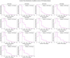 |
Fig. A.1. Control time distribution across different 7DT medium-band filters, considering that 90% of systems are unresolved. Median control times are represented by black vertical lines. |
Appendix B: Control time distribution of glSNe CC at different observing depths
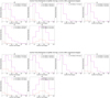 |
Fig. B.1. Control time distribution of glSNe CC at observing depths ≤ 22.04 for source redshifts zs ≤ 0.6 and zs > 0.6, considering (1) 50% and (2) 90% of systems are unresolved. Median control times are shown with black vertical lines. |
Appendix C: Annual detection rate of glSNe CC at different observing depths
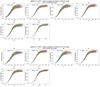 |
Fig. C.1. Annual detection rate of glSNe CC as a function of lens redshift calculated from 100 simulation realizations (individual realizations shown by colored lines). We present results at observational depths ≤ 22.04, accounting for (1) 50% and (2) 90% of systems being unresolved. |
All Tables
Best fit values for H0 with 1σ uncertainty at 10% precision in time-delay distance measurements of glSNe.
All Figures
|
Fig. 1. 7DT transmission curves for broad- and medium-band filters. |
| In the text | |
|
Fig. 2. Likelihood of lens candidates. |
| In the text | |
|
Fig. 3. Redshift distribution for selected lens galaxies and candidates zl, simulated source galaxies zs, and the ratio zl/zs. |
| In the text | |
|
Fig. 4. 7DT sky footprint (blue tile patterns) and location of selected lens galaxies and candidates (red dots). The approximate number of targeted 7DT fields covering the systems is 1125 tiles. |
| In the text | |
|
Fig. 5. Average detection rate of glSNe Ia for different 7DT medium-band filters and source redshifts zs≤0.6, assuming 90% of systems are unresolved. |
| In the text | |
|
Fig. 6. Upper panels: Control time distribution of glSNe Ia at different observing depths for source redshifts zs≤0.6 and zs>0.6, considering (1) 50% and (2) 90% of systems are unresolved. Black vertical lines indicate the median control times. Lower panel: Annual detection rate of glSNe Ia as a function of lens redshift calculated from 100 simulation realizations (individual realizations shown by colored lines). We present results at different observational depths, accounting for (1) 50% and (2) 90% of systems being unresolved. |
| In the text | |
|
Fig. 7. Reconstruction of the H0DL(z) function using GP reconstructions from SNe Ia dataset. |
| In the text | |
|
Fig. A.1. Control time distribution across different 7DT medium-band filters, considering that 90% of systems are unresolved. Median control times are represented by black vertical lines. |
| In the text | |
|
Fig. B.1. Control time distribution of glSNe CC at observing depths ≤ 22.04 for source redshifts zs ≤ 0.6 and zs > 0.6, considering (1) 50% and (2) 90% of systems are unresolved. Median control times are shown with black vertical lines. |
| In the text | |
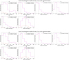 |
Fig. B.2. Same as Fig. B.1, but for observing depths ≤ 21.02. |
| In the text | |
|
Fig. C.1. Annual detection rate of glSNe CC as a function of lens redshift calculated from 100 simulation realizations (individual realizations shown by colored lines). We present results at observational depths ≤ 22.04, accounting for (1) 50% and (2) 90% of systems being unresolved. |
| In the text | |
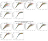 |
Fig. C.2. Same as Fig. C.1, but for observing depths ≤ 21.02. |
| In the text | |
Current usage metrics show cumulative count of Article Views (full-text article views including HTML views, PDF and ePub downloads, according to the available data) and Abstracts Views on Vision4Press platform.
Data correspond to usage on the plateform after 2015. The current usage metrics is available 48-96 hours after online publication and is updated daily on week days.
Initial download of the metrics may take a while.