| Issue |
A&A
Volume 691, November 2024
|
|
|---|---|---|
| Article Number | A178 | |
| Number of page(s) | 24 | |
| Section | Extragalactic astronomy | |
| DOI | https://doi.org/10.1051/0004-6361/202450420 | |
| Published online | 13 November 2024 | |
KASHz+SUPER: Evidence of cold molecular gas depletion in AGN hosts at cosmic noon
1
INAF–OAA, Osservatorio Astrofisco di Arcetri, largo E. Fermi 5, 50127 Firenze, Italy
2
Dipartimento di Fisica e Astronomia “Augusto Righi”, Università degli Studi di Bologna, Via P. Gobetti 93/2, 40129 Bologna, Italy
3
INAF–OAS, Osservatorio di Astrofisica e Scienza dello Spazio di Bologna, Via P. Gobetti 93/3, 40129 Bologna, Italy
4
European Space Agency (ESA), European Space Astronomy Centre (ESAC), Camino bajo del Castillo s/n, Villanueva de la Canada, E-28692 Madrid, Spain
5
Department of Physics & Astronomy, University College London, Gower Street, London WC1E 6BT, UK
6
Dipartimento di Fisica e Astronomia, Università di Firenze, Via G. Sansone 1, I-50019 Sesto F.no (Firenze), Italy
7
European Southern Observatory, Karl-Schwarzschild-Straße 2, D-85748 Garching bei Munchen, Germany
8
German Aerospace Center (DLR), Institute of Communications and Navigation, Wessling, Germany
9
School of Mathematics, Statistics and Physics, Newcastle University, Newcastle upon Tyne NE1 7RU, UK
10
Excellence Cluster ORIGINS, Boltzmannstraße 2, 85748 Garching bei München, Germany
11
Ludwig Maximilian Universität, Professor-Huber-Platz 2, 80539 München, Germany
12
Dipartimento di Fisica “G. Occhialini”, Universitá degli Studi di Milano-Bicocca, Piazza della Scienza 3, I-20126 Milano, Italy
13
Centre for Extragalactic Astronomy, Department of Physics, Durham University, South Road, Durham DH1 3LE, UK
14
Dipartimento di Fisica, Università di Trieste, Sezione di Astronomia, Via G.B. Tiepolo 11, I-34131 Trieste, Italy
15
INAF-Osservatorio Astronomico di Trieste, Via G.B. Tiepolo 11, I-34143 Trieste, Italy
16
Max-Planck-Institut für Extraterrestrische Physik (MPE), Giessenbachstraße 1, D-85748 Garching, Germany
17
Institute of Theoretical Astrophysics, University of Oslo, Postboks 1029, Blindern, 0315 Oslo, Norway
18
Space Telescope Science Institute, 3700 San Martin Drive, Baltimore, MD 21218, USA
19
European Southern Observatory, Alonso de Cordova 3107, Vitacura, Casilla, 19001 Santiago de Chile, Chile
20
Department of Physics, University of Oxford, Denys Wilkinson Building, Keble Road, Oxford OX1 3RH, UK
21
Centro de Astrobiología (CAB), CSIC–INTA, Cra. de Ajalvir Km. 4, 28850 Torrejón de Ardoz, Madrid, Spain
22
INAF – Osservatorio Astronomico di Roma, Via Frascati 33, 00040 Monte Porzio Catone, Roma, Italy
23
School of Physics and Astronomy, University of Southampton, Highfield SO17 1BJ, UK
24
Dipartimento di Matematica e Fisica, Universitá Roma Tre, Via della Vasca Navale 84, I-00146 Roma, Italy
25
Kavli Institute for Cosmology, University of Cambridge, Madingley Road, Cambridge CB3 OHA, UK
26
Cavendish Laboratory – Astrophysics Group, University of Cambridge, 19 JJ Thomson Avenue, Cambridge CB3 OHE, UK
27
INAF – Istituto di Astrofisica Spaziale e Fisica Cosmica Milano, Via A. Corti 12, 20133 Milano, Italy
⋆ Corresponding author; elena.bertola@inaf.it
Received:
17
April
2024
Accepted:
26
July
2024
The energy released by active galactic nuclei (AGN) has the potential to heat or remove the gas of the ISM, thus likely impacting the cold molecular gas reservoir of host galaxies at first, with star formation following as a consequence on longer timescales. Previous works on high-z galaxies, which compared the gas content of those without identified AGN, have yielded conflicting results, possibly due to selection biases and other systematics. To provide a reliable benchmark for galaxy evolution models at cosmic noon (z = 1 − 3), two surveys were conceived: SUPER and KASHz, both targeting unbiased X-ray-selected AGN at z > 1 that span a wide bolometric luminosity range. In this paper we assess the effects of AGN feedback on the molecular gas content of host galaxies in a statistically robust, uniformly selected, coherently analyzed sample of AGN at z = 1 − 2.6, drawn from the KASHz and SUPER surveys. By using targeted and archival ALMA data in combination with dedicated SED modeling, we retrieve CO and far-infrared (FIR) luminosity as well as M* of SUPER and KASHz host galaxies. We selected non-active galaxies from PHIBBS, ASPECS, and multiple ALMA/NOEMA surveys of submillimeter galaxies in the COSMOS, UDS, and ECDF fields. By matching the samples in redshift, stellar mass, and FIR luminosity, we compared the properties of AGN and non-active galaxies within a Bayesian framework. We find that AGN hosts at given FIR luminosity are on average CO depleted compared to non-active galaxies, thus confirming what was previously found in the SUPER survey. Moreover, the molecular gas fraction distributions of AGN and non-active galaxies are statistically different, with the distribution of AGN being skewed to lower values. Our results indicate that AGN can indeed reduce the total cold molecular gas reservoir of their host galaxies. Lastly, by comparing our results with predictions from three cosmological simulations (TNG, Eagle, and Simba) filtered to match the properties of observed AGN, AGN hosts, and non-active galaxies, we confirm already known discrepancies and highlight new discrepancies between observations and simulations.
Key words: galaxies: active / galaxies: evolution / galaxies: high-redshift / galaxies: ISM / quasars: general / submillimeter: ISM
© The Authors 2024
 Open Access article, published by EDP Sciences, under the terms of the Creative Commons Attribution License (https://creativecommons.org/licenses/by/4.0), which permits unrestricted use, distribution, and reproduction in any medium, provided the original work is properly cited.
This article is published in open access under the Subscribe to Open model. Subscribe to A&A to support open access publication.
1. Introduction
The sphere of gravitational influence of supermassive black holes (SMBHs) is spatially limited to the innermost regions of galaxies (∼10 pc for a 108 M⊙ black hole; Alexander & Hickox 2012). However, SMBH accretion can release large amounts of energy that, if efficiently coupled to the surrounding material, allows active galactic nuclei (AGN) to shape galaxy growth by heating, exciting, and/or removing the gas of the interstellar medium (ISM). Such an interplay between AGN activity and the life of galaxies is referred to as AGN feedback (e.g., Silk & Rees 1998; Fabian 2012). Astronomers have found much observational evidence for a connection between observational and physical properties of the central AGN and its host galaxy (e.g., Strateva et al. 2001; McConnell et al. 2011; Rodighiero et al. 2015), as also predicted by theoretical models (e.g., Somerville et al. 2008; Lapi et al. 2014; Costa et al. 2018), leading to what is called the AGN–galaxy co-evolution scenario. However, we still lack a full understanding of AGN feedback despite its importance (e.g., Kormendy & Ho 2013; Harrison 2017; Harrison et al. 2018; Ward et al. 2022), for instance whether galaxy evolution is influenced by AGN activity as a whole, whether AGN-driven winds and jets are key properties in driving AGN feedback effects, or whether we are using sensitive observational tracers for AGN feedback. AGN feedback is believed to be highly dominant when both cosmic SMBH growth and star formation rate (SFR) were at their peaks (cosmic noon, z ≃ 1 − 3; e.g., Madau & Dickinson 2014; Aird et al. 2015). Hence, sources at cosmic noon are the most promising and most informative targets to investigate AGN feedback, both in terms of causes (e.g., AGN-driven winds and jets) and effects (e.g., reduced gas fraction and disturbed gas kinematics in AGN hosts).
One way to test the impact of AGN feedback on the host galaxy is to observe its molecular gas content and conditions. In particular, the Schmidt–Kennicutt law (Schmidt 1959; Kennicutt 1989) is a fundamental relation that links the molecular gas content and the level of star formation (SF) in galaxies, that is often used in its integrated form (i.e., the global SFR of galaxies vs. their total molecular mass; (e.g., Carilli & Walter 2013; Sargent et al. 2014; Perna et al. 2018; Bischetti et al. 2021; Circosta et al. 2021). If AGN influence the evolution of galaxies as a whole (e.g., Fabian 2012; Harrison 2017; Harrison & Ramos Almeida 2024), they will reasonably impact the molecular gas reservoir first, and then, consequently, SF on longer timescales. In addition to addressing AGN feedback as “caught in the act” (i.e., AGN-driven outflows or radio jets), comparative studies of the molecular gas properties in AGN host galaxies and matched non-active galaxies (i.e., galaxies not hosting an AGN) can shed light on the impact of AGN on galaxy evolution, regardless of whether outflows are concurrently detected in a given source.
A powerful proxy for measuring the molecular content of galaxies is represented by carbon monoxide (CO), the second most abundant molecule after H2, and hence the primary tracer of molecular gas (e.g., Carilli & Walter 2013; Hodge & da Cunha 2020). The molecular gas mass can be derived from the luminosity of the ground state transition CO(1–0) (MH2 = αCOL′CO(1 − 0)). However, the value of αCO has to be assumed, and it is very uncertain as it depends on different quantities, for instance the distance from the main sequence (MS, Elbaz et al. 2007; Noeske et al. 2007) and the metallicity (e.g., Accurso et al. 2017). The value calibrated on the Milky Way (αCO = 4 M⊙ (K km s−1 pc2)−1; Bolatto et al. 2013) can be a good approximation for regular star-forming galaxies (Carilli & Walter 2013), while a lower value of αCO = 0.8 − 1 M⊙ (K km s−1 pc2)−1 (Downes & Solomon 1998; Solomon & Vanden Bout 2005; Calistro Rivera et al. 2018; Amvrosiadis et al. 2023) or αCO = 1.8 − 2.5 M⊙ (K km s−1 pc2)−1 (Cicone et al. 2018; Herrero-Illana et al. 2019; Montoya Arroyave et al. 2023) could be more representative for high-z submillimeter (sub-mm) galaxies, which usually have an extremely dense ISM and often intense SF activity (e.g., Birkin et al. 2021). Observations of massive MS galaxies at cosmic noon resulted in an αCO = 3.6 M⊙ (K km s−1 pc2)−1 (e.g., Daddi et al. 2010a; Genzel et al. 2015).
Measuring the ground transition of CO is not always possible, especially at high redshift. However, observations of CO transitions from higher-J levels can be converted to the CO(1–0) flux by assuming a CO spectral line energy distribution (CO-SLED), which expresses the relative strength of the CO rotational lines as a function of the quantum number J (e.g., Pozzi et al. 2017; Mingozzi et al. 2018; Kirkpatrick et al. 2019; Boogaard et al. 2020; Valentino et al. 2021; Pensabene et al. 2021; Esposito et al. 2022; Molyneux et al. 2024). Even though AGN mostly contribute to high-J levels, CO ladders of AGN hosts and non-active galaxies are seen to vary also at J < 5, despite the large associated uncertainties, with AGN showing higher ratios that increase for increasing AGN luminosity (Carilli & Walter 2013; Kirkpatrick et al. 2019; Vallini et al. 2019; Boogaard et al. 2020).
Results regarding the effects of AGN on the molecular gas phase are controversial and seem to hint at a dichotomy between low-z and high-z scenarios. With regard to the integrated properties of galaxies, AGN hosts in the local Universe are usually similar to non-active galaxies (e.g., Rosario et al. 2018; Koss et al. 2021; Salvestrini et al. 2022, but see also Mountrichas et al. 2024) or are even richer in gas, in the sense that more powerful AGN are hosted in host galaxies that are more gas-rich (e.g., Vito et al. 2014; Husemann et al. 2017). However, significant effects of negative AGN feedback are seen in local AGN hosting molecular outflows (Fiore et al. 2017). Additionally, some results hint at enhanced SF efficiencies in both local and high-z AGN hosts possibly linked to large molecular gas reservoirs (e.g., Shangguan et al. 2020a; Jarvis et al. 2020; Bischetti et al. 2021). Spatially resolved studies of local galaxies have revealed gas depletion in the nuclear regions of AGN hosts, and not on galactic scales (Sabatini et al. 2018; Rosario et al. 2019; Fluetsch et al. 2019; Feruglio et al. 2020; Ellison et al. 2021; García-Burillo et al. 2021, 2024; Zanchettin et al. 2021; Ramos Almeida et al. 2023), with indications that the central SF activity (within a few 100 pc) is indeed reduced due to the presence of AGN, while the galaxy-wide SFR is unaffected (e.g., Sánchez et al. 2018; Lammers et al. 2023, but see also Molina et al. 2023 and Bessiere & Ramos Almeida 2022, who find enhanced SF activity in the proximity of the AGN). At high redshift the observed impact of AGN on the molecular ISM of their hosts is debated. Several studies find that AGN hosts are significantly CO-depleted when compared to control samples of non-active galaxies, either in terms of gas fraction1 or of depletion timescales (e.g., Brusa et al. 2016, 2018; Kakkad et al. 2017; Perna et al. 2018; Bischetti et al. 2021, but see also Herrera-Camus et al. 2019; Spingola et al. 2020). Instead, other studies find little (e.g., Circosta et al. 2021, hereafter, C21) to no significant difference between the gas fraction of non-active galaxies and AGN hosts (e.g., Valentino et al. 2021), and some other works find no clear link between gas content and AGN power (e.g., Kirkpatrick et al. 2019). An additional issue in comparing the properties of AGN hosts and non-active galaxies resides in the intrinsic variability of AGN and their flickering activity (Harrison 2017; Harrison & Ramos Almeida 2024), which can also affect the distinction of galaxies that host and that do not host an AGN based on when the system was targeted, for instance, in X-rays.
Predictions from cosmological simulations also seem to be controversial. In particular, Ward et al. (2022) recently analyzed the output of three key cosmological simulations (Illustris-TNG, hereafter TNG; Springel et al. 2018; Pillepich et al. 2018; Naiman et al. 2018; Nelson et al. 2018; Marinacci et al. 2018; EAGLE, Crain et al. 2015; Schaye et al. 2015; Simba, Davé et al. 2019) applying the same methods employed to analyze observations of galaxies and AGN hosts. Considering samples of local and z = 2 targets, the authors conclude that none of the selected simulations predicts strong negative correlations between AGN power and molecular gas fraction or specific SFR (sSFR = SFR/M*). Conversely, powerful AGN seem to preferentially reside in gas-rich, highly star-forming galaxies, whereas gas-depleted and quenched fractions are higher in the control samples of regular galaxies than for the AGN hosts. Ward et al. (2022), however, argue that there is a quantifiable difference among the predictions of the three selected simulations, and that the bolometric luminosity range covered by simulations and observational efforts barely overlap, especially at cosmic noon. This is mainly due to the difficulty in reproducing sizable samples of high-luminosity AGN (Lbol ≳ 1043.5 erg s−1 at z = 0 and Lbol ≳ 1045 erg s−1 at z = 2) in cosmological simulations, since they are rare and too short-lived to be captured in the simulated volumes, and to the observational cost of observing sizable samples of less luminous AGN (e.g., Lbol ≲ 1044 erg s−1 at z > 1).
The dichotomy between results on local and high-z targets, and between different samples of high-z sources, could arise from selection effects. High-z studies usually rely on a few high-luminosity ( ) and heterogeneous targets, both because high-power AGN are the best candidates to produce efficient feedback (e.g., Fiore et al. 2017) and because of the challenging observations required for distant objects. Two surveys of X-ray-selected AGN were recently conceived to provide multiwavelength studies of AGN samples blindly selected with respect to the presence of ionized outflows or jets at cosmic noon: KASHz (KMOS AGN Survey at High redshift, PI: D. Alexander; Harrison et al. 2016; Scholtz et al., in prep.) at z = 0.6 − 2.6 and SUPER (SINFONI Survey for Unveiling the Physics and Effect of Radiative feedback, PI: V. Mainieri; Circosta et al. 2018, hereafter, C18) at z = 2 − 2.5. The aim of both surveys is the study of the interplay between AGN and galaxy evolution in terms of AGN-driven ionized winds, traced through [OIII] emission lines, and the properties of the host galaxy (see Sect. 2). SUPER relied on adaptive-optics-assisted, spatially resolved studies of ionized gas, which require longer exposures, leading to a reduced sample size and sparser sampling of AGN with log(Lbol/erg s−1) < 45 compared to the KASHz survey, with its larger sample size and lower bolometric luminosity cut. In this context, the different observational capabilities and selection criteria make KASHz and SUPER complementary surveys, and thus using them together allows us to capitalize on their strengths.
As part of the SUPER survey, C21 provided the first systematic analysis of the molecular gas content of AGN host galaxies at z ≃ 2 through a dedicated follow-up in CO(3–2) with the Atacama Large Millimeter Array (ALMA). With robust measurements of physically relevant quantities (SFR, Mgas) traced through observational proxies (LFIR, L′CO(3 − 2)), the authors find hints of negative AGN feedback effects in their sample. However, the sample size of SUPER ALMA AGN did not allow us to determine whether such hints of gas depletion were indicative of less prominent AGN feedback effects in moderate luminosity AGN or due to a large fraction of upper limits combined with a limited sample size. As Figure 1 shows, combining SUPER targets with KASHz AGN allows a robust sampling of moderate-luminosity AGN (44 < log(Lbol/erg s−1) < 46), still covering a wide range in AGN bolometric luminosity by means of the different sample selection criteria (see Fig. 1, but also Fig. 1 of C18).
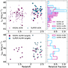 |
Fig. 1. Luminosity versus redshift distribution of the AGN samples used in this work. Top: intrinsic 2–10 keV rest-frame X-ray luminosity LX vs. redshift z distribution of the full KASHz (purple pentagons) and SUPER (blue circles) surveys. SUPER ALMA targets are from C21. The side panel shows the density distribution of SUPER (blue) and KASHz (purple) targets. Bottom: bolometric luminosity LBol vs. redshift z distribution of the AGN targeted by ALMA and included in this work. For the KASHz (purple pentagons) and SUPER (blue circles) targets included in this panel, the bolometric luminosity was derived from SED fitting in this work (see Appendix D), in C18, and in C21. The side panel shows the density distribution of the samples. The black dots mark the six targets discarded because they were missing at least one parameter of interest for our analysis; the white dots mark the three targets that do not allow fgas to be computed. |
The aim of this work is to investigate the molecular gas properties of a statistically robust, consistently selected, coherently analyzed sample of AGN at cosmic noon (z = 1 − 2.6) available in the ALMA archive, improving the sampling of the  bolometric range. We built upon the methods and analysis of C21, and built our sample combining SUPER ALMA AGN with targets from the KASHz survey (see Sect. 2). The control sample of non-active galaxies is presented in Sect. 3. The ALMA data selection and reduction of KASHz targets is presented in Sect. 4 and Appendix C, while the SED fitting and photometry collection of both SUPER and KASHz AGN are described in Appendix D. We then apply a quantitative analysis in the Bayesian framework developed by C21 to compare our enlarged AGN sample with the control sample of non-active galaxies in Sect. 5. In Sect. 6 we compare our observed sample with the output of cosmological simulations. Results are discussed and summarized in Sects. 7 and 8. We assume a flat ΛCDM cosmology (Planck Collaboration VI 2020), with H0 = 67.7 km s−1 Mpc−1 and Ωm, 0 = 0.31 throughout the paper.
2. Sample selection
To build a robust sample of moderate- to high-luminosity AGN (log(Lbol/erg s−1)≃44 − 47), we considered all the SUPER ALMA targets presented in C21 and complemented them with archival ALMA observations targeting the CO emission with J < 5 (CO(1–0), CO(2–1), CO(3–2), CO(4–3)) of KASHz AGN (see Sects. 2.1 and 4.1, Appendix C, and Table E.1). The other needed parameters for our analysis (mainly M* and LFIR) were estimated from SED fitting performed with CIGALE (Boquien et al. 2019; Yang et al. 2020) using the most up-to-date multiwavelength broadband photometry released by the deep field collaborations (see Appendix D). Table 1 summarizes source ID, coordinates, redshift and parent sample. Figure 1 shows the LX versus z distribution of the full KASHz and SUPER survey samples. We also show the Lbol versus z distribution of the AGN used in this work (i.e., ALMA targets from KASHz and SUPER) as derived from SED fitting (see Appendix C).
Summary of the AGN sample
For the analysis presented in Sect. 5, we discarded six AGN from the SUPER and KASHz ALMA samples because they were missing at least one of the parameters of interest needed for our analysis (M* or LFIR; we flag these targets with an asterisk in Table E.2 and in the bottom panel of Fig. 1). These six targets are extremely bright broad-line AGN with sparse or missing far-infrared (FIR) photometry coverage. A reasonable decoupling of AGN and galaxy emission in the SED fitting is thus not possible, and also hampers the determination of meaningful upper limits for stellar mass and FIR luminosity of the host galaxy (C18; C21).
2.1. KASHz survey
The KASHz survey (Harrison et al. 2016, Scholtz et al., in prep.) is a VLT/KMOS GTO survey of X-ray-selected AGN (PI: D. Alexander), built with the aim of investigating the impact of AGN feedback on the ionized gas phase as traced by the Hβ, [OIII]λ5007, Hα, [NII]λ6583, and [SII]λλ6717, 6730 optical emission lines. The final catalog of the survey will be presented in Scholtz et al. (in prep.), alongside the results from the spectral analysis of the ionized gas emission. We summarize here some important properties of the survey sample.
The KASHz survey totals ≃230 AGN, spanning the redshift range z = 0.6 − 2.6 and the LX range log(LX/erg s−1) = 41 − 45.4, which corresponds to a bolometric luminosity range of  , based on the bolometric correction derived by Duras et al. 2020. Near-IR (NIR) spectroscopic data is available for all KASHz targets, predominantly from our KMOS program, but also including archival SINFONI data. KASHz targets were drawn from five different X-ray deep fields: i) Chandra Cosmic evolution survey fields (C-COSMOS and COSMOS-Legacy; Civano et al. 2016; Marchesi et al. 2016, name convention: cid_ID and lid_ID); ii) Chandra Deep Field South (CDFS; Luo et al. 2017, name convention: cdfs_ID); iii) Subaru/XMM-Newton Deep Survey (SXDS; Ueda et al. 2008; Akiyama et al. 2015, name convention: sxds_ID); iv) Chandra Legacy Survey of the UKIDSS Ultra Deep Survey field (X-UDS; Kocevski et al. 2018, name convention: xuds_ID); v) SSA22 protocluster field (Lehmer et al. 2009, name convention: ssa22_ID). Based on our spectroscopic redshift identification using NIR spectra, we confirm or update the redshift listed in the parent X-ray survey catalogs and the respective rest-frame X-ray properties, as described in Appendix A.
By dropping the AGN at z < 1, the KASHz survey comprises ≃200 sources of which only ∼10% were targeted in CO at J < 5 and are thus included in this work (see Sect. 4.1). We present in Sect. 4 and Appendix C the reduction and analysis of ALMA data of KASHz AGN. Through dedicated SED fitting (see Appendix D), we measure for KASHz ALMA targets stellar masses in the log(M*/M⊙)≃10.3 − 11.8 range, FIR luminosities in the log(LFIR/erg s−1)≃44.3 − 46.2 range (see Table E.2), and bolometric luminosity in the log(Lbol/erg s−1)≃44.3 − 46.6 range.
2.2. SUPER survey
The SUPER survey2 total sample includes 48 X-ray-selected AGN at z = 2 − 2.5 with  , without prior knowledge of the presence of AGN-driven outflows (C18, C21). This SINFONI Large Program allowed us to provide a spatially resolved systematic study of the occurrence and properties of ionized AGN-driven winds (Kakkad et al. 2020; Tozzi et al. 2024), to investigate the effects of AGN activity on the available molecular gas reservoir using ALMA Band 3 observations of the CO(3–2) transition (C21), and to investigate the impact of ionized outflows on SFR (Kakkad et al. 2023) in cosmic noon host galaxies. Targets were drawn from both deep and large-area X-ray surveys: COSMOS-Legacy, CDFS, XMM-Newton XXL survey (XMM-XXL, Pierre et al. 2016, name convention X_N_ID), Stripe 82 X-ray survey (Stripe82, LaMassa et al. 2016; Ananna et al. 2017, name convention S82X_ID). The sample also includes AGN selected from the WISE/SDSS selected Hyper-luminous quasars sample (WISSH, Bischetti et al. 2017) based on their redshift and X-ray luminosity, as obtained by the WISSH collaboration from proprietary X-ray observations by Chandra and XMM-Newton (Martocchia et al. 2017). Given the similar selection strategy and the common goal, the SUPER survey can be considered the high-resolution version of KASHz at z ≃ 2 − 2.5. In fact, there are 14 AGN that are shared between the two samples3 We refer to C21 for the analysis and results of the ALMA sample of SUPER AGN (27 targets), and to C18 and C21 for the SED fitting of ALMA targets drawn from the XMM-XXL field. The updates in dedicated SED fitting of SUPER AGN selected from CDFS and COSMOS are presented in Appendix D. We measure for SUPER ALMA targets stellar masses in the log(M*/M⊙)≃10.2 − 11.7 range, FIR luminosity in the log(LFIR/erg s−1)≃44.3 − 46.4 range, and bolometric luminosity in the log(Lbol/erg s−1)≃44.7 − 46.9 range (see Table E.2).
3. Control sample of non-active galaxies
We built the comparison sample using literature measurements of non-active galaxies. We selected star-forming non-active galaxies from the Plateau de Bure high-z Blue Sequence Survey catalog (PHIBSS, Tacconi et al. 2018), which has the aim of assessing the gas properties of galaxies across cosmic time, employing a sample of 1444 targets placed at z = 0 − 4.4. Each target was complemented with estimates of the molecular gas mass, as traced by CO emission (including CO non-detections), and FIR luminosity, as measured either from SED fitting or from the dust continuum luminosity. We include the ALMA/NOEMA survey of sub-mm galaxies in the COSMOS, UDS, and extended CDFS (ECDFS) fields by Birkin et al. (2021) and the non-active galaxies of ASPECS (Boogaard et al. 2020, and references therein), to better sample the higher end and the lower end, respectively, of the stellar mass range spanned by our AGN host galaxies. The PHIBSS project includes the pilot ALMA program of ASPECS that was presented in Decarli et al. (2016); for those galaxies, we used the latest estimates provided by the ASPECS survey, as reported in Boogaard et al. (2020).
We included in the control sample all the non-active galaxies observed in CO(3–2) and CO(2–1), as obtained by ALMA and NOEMA, and retrieve the CO(1–0) using r21 = 0.6 and r31 = 0.5 (i.e., excitation ratios) commonly found for star-forming galaxies in the same redshift range as our AGN (Daddi et al. 2010b; Tacconi et al. 2013; Kakkad et al. 2017). CO fluxes were retrieved from the literature (Boogaard et al. 2020; Birkin et al. 2021) or were provided by the PHIBSS collaboration (Tacconi, priv. comm.) since Tacconi et al. (2018) only report the final molecular gas masses. We also checked the nature of the galaxies in the control sample and excluded those that are flagged as AGN. We did not include such targets in our AGN sample because their stellar masses and SFRs were not corrected accounting for the AGN contribution and could thus be overestimated, and because they are identified as AGN with methods different from ours.
All the galaxies in the comparison sample have available estimates of stellar mass and FIR luminosity. However, the SFR of a small subsample of PHIBSS galaxies was estimated from Hα fluxes. Based on the reasonable agreement between the SFRs derived from Hα and from the FIR for MS galaxies at cosmic noon (within ≃0.4 dex; Rodighiero et al. 2014; Puglisi et al. 2016; Shivaei et al. 2016), we converted such SFRs to FIR luminosity applying the Kennicutt (1998) relation corrected for a Chabrier (2003) IMF (i.e., reduced by 0.23 dex).
We built the control sample of non-active galaxies as follows. First, we divided our AGN sample into two redshift bins (z = 1 − 1.8 and z = 1.8 − 2.55), which we used as redshift constraints for the match in stellar mass and SFR to take into account the evolution of the MS with redshift (e.g., Genzel et al. 2015; Tacconi et al. 2018). For each redshift bin, we only considered non-active galaxies within the same stellar mass range covered by our AGN host galaxies within the uncertainties (log M*/M⊙ ≃ 10 − 12), and we further divided the samples in bins of stellar mass of 0.5 dex width. For each stellar mass bin, we then selected all those non-active galaxies with a SFR consistent with (within +0.2 dex to consider the uncertainties) or lower than that of AGN hosts in a given mass (and redshift) bin, so as to also account for the SFR upper limits in the AGN sample. We show in Fig. 2 the comparison of our AGN (in red) and control sample (in blue) in terms of SFR versus M*. Figure B.1 in Appendix B shows the same comparison in the low-z and high-z bins. Figures 2 and B.1 also show the distribution of M* and SFR both for AGN hosts and non-active galaxies for illustration purposes since the upper limits are considered, for these plots only, at face value. A robust comparison of the distribution of SFR and M* applying the hierarchical method described in Sect. 5.2 and the Kolmogorov–Smirnov (KS) test is presented in Appendix B. We find that AGN hosts and non-active galaxies selected as presented in this section are consistent with being drawn from the same distribution for the stellar mass in all redshift bins (low-z, high-z, total) and for the SFR in the low-z bin and total redshift range. However, they are significantly different for SFR distribution of the high-z bin (p-value ≃ 1%). The galaxy database used to build the control sample is missing non-active galaxies with CO observations that fall below the MS at z > 1.8 (ΔMS < −0.5 dex; see Fig. B.1, bottom) due to the rareness of low-SFR star-forming galaxies not hosting AGN and to the time-consuming observations required to target their molecular phase. Since not even dust-continuum observations cover non-active galaxies in such a region of the MS (e.g., Tacconi et al. 2020), we ran our comparative analysis twice: we compare the full AGN and non-active galaxy samples built as described in this section and in Sect. 2, and then we compared them again excluding those AGN lacking a match in the control sample in the high-z bin (i.e., z > 1.8, log(M*/M⊙) > 11, log(SFR/M⊙ yr−1) < 2; see Fig. B.1) and those galaxies in the low-z bin that do not have a match in the AGN sample (i.e., z < 1.8, log(M*/M⊙) < 10.5, log(log(SFR/M⊙ yr−1) < 1.5; see Fig. B.1) as a sanity check of our results.
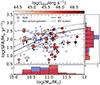 |
Fig. 2. Comparison of star formation rate and stellar mass of the AGN host galaxies (red circles) and the non-active galaxies of the control sample (blue squares). The red circles are color-coded based on their AGN bolometric luminosity, as retrieved from SED fitting from this work or from the literature. The solid line is the MS at z = 2 from Schreiber et al. (2015) and dashed lines show its scatter (equal to 0.3 dex). The distribution of SFR (right) and M* (bottom) for AGN (red) and non-active galaxies (blue) in the two side panels are intended for illustration purposes only since the upper limits are considered at face value. A robust comparison of the distribution of SFR and M* applying the hierarchical method described in Sect. 5.2 is presented in Fig. B.2. |
4. ALMA observations of KASHz targets
4.1. Data selection
We mined the ALMA archive for observations of KASHz AGN at 1 < z < 2.6 (202 sources). We narrowed our query to ALMA Band 3, 4, or 5 since these are the bands that cover low-J CO transitions (Jup = 2, 3, 4), most suitable for deriving the total molecular gas masses. ALMA observations in Band 3 and 4 are available for ≃10% of the KASHz sample (to which we also refer as the ALMA KASHz sample), for a total of 22 ALMA fields from 13 ALMA projects. No suitable ALMA data is available in Band 5. We report in Table C.1 all observations analyzed in this work. We refer to the results and analysis in C21 for those KASHz targets shared with SUPER that are already presented in C21 (marked in Table E.1). Some KASHz AGN were observed multiple times in more than one CO transition (cdfs_427, cdfs_587, cdfs_614) or in the same transition at different angular resolutions (cdfs_794, cdfs_587). For these targets we considered the ALMA observation targeting the CO transition at the lowest J and/or with the largest beam size to maximize the sensitivity per beam and simultaneously minimize the resolution in order to best recover the total CO flux. The only exception is cdfs_794; since this is a merger system observed twice in CO(3–2) in low and high angular resolution setup, we selected the observation at the highest resolution (Calistro Rivera et al. 2018) to ensure no contamination from the nearby companion. Moreover, we excluded cdfs_718, the brightest target in the ALMA Spectroscopic Survey in the Hubble Ultra Deep Field (ASPECS ID 1 mm.1; Decarli et al. 2019; González-López et al. 2019; Aravena et al. 2019; Boogaard et al. 2020), from the KASHz ALMA sample, due to the presence of a dust lane as seen in the HST data (Boogaard et al. 2019) that contaminates the FIR emission, thus preventing a good determination of its FIR parameters and decoupling of AGN and host components in the SED fitting.
There are 10 observations that target the CO(2–1) line, 15 for the CO(3–2), and 3 for the CO(4–3). We also present here the CO(3–2) NOEMA data of J1333+1649 (project code S21CG, PI Mainieri), a SUPER AGN (drawn from the WISSH sample) that was not previously included in C21 because it was subsequently observed. Almost all the other AGN in KASHz and SUPER are equatorial or in the southern hemisphere to be observable by VLT. As a sanity check, we also queried the IRAM archive at the Centre de Données astronomiques de Strasbourg for NOEMA observations of the rest of sample; however, there are no public NOEMA observations covering the CO emission lines of our targets.
4.2. CO emission of KASHz AGN
We present here and in Appendix C the data reduction and analysis of the ALMA archival observations analyzed in this work. We refer to the results of C21 for the KASHz ALMA targets that are shared with SUPER and that were previously analyzed. We list all the KASHz ALMA targets, including those shared with SUPER, in Table E.1, along with information on the parent X-ray deep field, AGN type, redshift, X-ray intrinsic photon index, X-ray absorption column density, and absorption-corrected X-ray luminosity in the 2–10 keV rest-frame band with a flag indicating how we computed it.
We retrieved the calibrated measurement sets using the dedicated service provided by the European ALMA Regional Center. We produced continuum maps and continuum-subtracted spectral cubes using the task tclean in CASA 6.4 (CASA Team 2022), ran in “mfs” or “velocity” mode, respectively. The continuum was identified using all the spectral windows available in the ALMA observation, masking the channels with line emission, and then subtracted with the uvcontsub CASA task. We imaged all fields using a natural weighting scheme of the visibilities and pixel size of ≃1/5 of the beam full width at half maximum (FWHM), with the aim of maximizing the sensitivity of our data. We produced the final cubes by setting a channel width that allows sampling the line FWHM with at least seven spectral resolution elements, chosen as the best trade-off to sample the line profile, while maintaining a good signal-to-noise ratio. CO fluxes were estimated by fitting the 1D spectrum, and validated by the comparison with the spatially integrated line flux and two-dimensional fits of the line velocity-integrated maps (0th order moment). Non-detections were defined as sources with signal-to-noise ratio S/N < 3 in the velocity-integrated maps. The steps and details of the ALMA data analysis are presented in Appendix C, and the results in Table E.3. We show the velocity-integrated maps and spectra of cid_108 as example in Fig. 3. Those of the rest of the sample are available on Zenodo4.
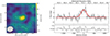 |
Fig. 3. CO line velocity-integrated emission map (left) and spectrum (right) of cid_108. The solid contour levels in the left panels start at 2σ and increase linearly. The dashed contours indicate the [−3,−2]×σ level. The beam of each observation is shown by the gray ellipse in the bottom left corner of each map. CO maps and spectra of the rest of the AGN sample are available on Zenodo at the following link: https://doi.org/10.5281/zenodo.13149280 |
Since our sample is heterogeneous in terms of targeted CO transition (CO(2–1), CO(3–2), CO(4–3)), we convert the measured CO fluxes to the CO(1–0) transition assuming the line ratios measured for a sample of IR-selected AGN up to z ≃ 4 (r41 = 0.37 ± 0.11, r31 = 0.59 ± 0.18, r21 = 0.68 ± 0.17, Kirkpatrick et al. 2019), and derive the CO(1–0) line luminosity as
![$$ \begin{aligned} L\prime _{\rm CO}[\mathrm{K\,km\,s^{-1}\,pc^2}] = 3.25\times 10^7S\Delta v\frac{D^2_{\rm L}}{(1+z)^3\nu _{\rm obs}^2} ,\end{aligned} $$](/articles/aa/full_html/2024/11/aa50420-24/aa50420-24-eq5.gif)
where SΔv is the line velocity-integrated flux in Jy km s−1, DL is the luminosity distance in Mpc, and νobs is the observed centroid frequency of the line in GHz (e.g., Carilli & Walter 2013). The uncertainty on L′CO is computed from error propagation of the uncertainties on the measured fluxes and the errors on the CO ladder. The latter are the larger source of uncertainty, and thus dominate the error on L′CO. We note that the CO ladder used for AGN is consistent with that used for the non-active galaxies of the control sample, and thus our analysis is set in a conservative framework.
Table E.3 summarizes all the values of interest derived from the ALMA data analysis of the KASHz ALMA targets presented in this work: CO properties and dust-continuum measurements, the chosen weighting scheme, the beam of the ALMA cubes and continuum maps, the channel width of the final cubes, the mean rms of the final cubes and velocity-integrated maps, and CO(1–0) luminosity. We apply the same CO ladder to convert the CO(3–2) luminosity of SUPER ALMA AGN measured by C21 to L′CO, which we report in Table E.2.
5. Molecular gas properties of AGN at cosmic noon
In this section we present our comparative quantitative analysis of the cold molecular gas content of AGN host galaxies and non-active galaxies at z = 1 − 2.6. The AGN sample selection is described in Sect. 2 and the control sample of non-active galaxies was built as described in Sect. 3 (see Fig. 2). We address the effects of AGN feedback on the properties of host galaxies at z = 1 − 2.6 by assessing whether they differ from the respective control sample in terms of i) CO versus FIR luminosity; ii) distribution of molecular gas fraction, for which we consider the observational proxy fgas = L′CO/M*; iii) CO luminosity versus stellar mass; and iv) molecular gas fraction (i.e., L′CO/M*) versus stellar mass. Moreover, we also ran the analysis removing the AGN at z > 1.8 that fall below the MS and do not have a match in the control sample, and galaxies in the low-redshift bin without a counterpart in the AGN sample (i.e., below the MS; see Sect. 3 and Appendix B). We anticipate that the results obtained excluding such AGN and non-active galaxies are consistent with those of the full samples.
The total AGN sample comprises 46 AGN and presents a CO detection rate of ≃50%. Roughly half of the AGN have a constrained LFIR and about ≃44% have an upper limit for both quantities. All but five AGN have constrained stellar mass, of which three (cid_178, cid_1605, cid_467) are undetected in CO, and thus do not allow a limit on their gas fraction to be derived. We summarize the properties of KASHz and SUPER ALMA AGN in Table E.2. The control sample totals 98 galaxies, with a CO detection rate of ≃90%.
We performed our analysis within a Bayesian framework as presented in C21, which allows us to take into account the upper (and lower) limits on both dependent and independent variables. There is only one main difference in this work with respect to C21: the KASHz AGN are heterogeneous in terms of targeted CO transition, while SUPER AGN were all observed in CO(3–2). We relied on the CO(1–0) luminosity by assuming a CO SLED that we uniformly applied to the CO measurements of KASHz and SUPER AGN (see Sect. 4.2) and a second one for the star-forming galaxies of the control sample (see Sect. 3). Our analysis remains free of the additional uncertainties inherent to the αCO conversion factor and the conversion of FIR luminosity into SFR. Figures in this section also show the molecular mass axis, derived assuming αCO = 3.6 M⊙/(K km s−1 pc2), but they are for illustration purposes only since we only consider L′CO in our quantitative analysis.
5.1. CO versus FIR luminosity
In this section we quantify whether AGN host galaxies and non-active galaxies at cosmic noon follow a different distribution in the CO and FIR luminosity parameter space (i.e., an observational proxy of the integrated Schmidt-Kennicutt law). We apply the Bayesian method to produce bisector fits as developed by C21, which we briefly explain here. We fit a linear model to the data applying the ordinary least-squares (OLS) bisector fit method (Isobe et al. 1990); that is, we take into account the uncertainties on L′CO and LFIR separately to consider the upper limits on both quantities, and then we derive the bisector of the two lines in a Bayesian framework, assuming uniform priors for free parameters. When building the likelihood function of constrained values, we assumed their uncertainties as Gaussian distributed. Upper limits were included in the likelihood function as error functions (see, e.g., Lamperti et al. 2019), built integrating the Gaussian likelihood from minus infinity to the value of the upper limit: 3σ for both CO and FIR luminosity. We then sample the yielded likelihood function through the emcee library (Foreman-Mackey et al. 2013), a Python implementation of the invariant MCMC (Markov chain Monte Carlo) ensemble sampler of Goodman & Weare (2010). We derive the marginalized posterior distribution by sampling the posterior distribution in the parameter space, using the best fit obtained through the Python module scipy.optimize (Virtanen et al. 2020) as an initial guess. We include an additional intrinsic scatter to the relation as a third free parameter to account for the possibility of underestimated uncertainties, given the wide range spanned by our sources (∼2.5 dex both in L′CO and in LFIR). The best-fit parameters were then derived as the median of the sampled marginalized posterior distribution of the OLS best-fit parameters, assigning as uncertainties the 16th and 84th percentiles. The final values of slope (a) and intercept (b) for the bisector fit were then derived from the OLS best-fit values following Isobe et al. (1990). The fits were performed by normalizing the x and y variables to the mean of the range covered by the data points so to reduce the correlation between the best-fit parameters.
Best-fit parameters for AGN and non-active galaxies.
Figure 4 shows the results in the integrated Schmidt–Kennicutt plane. We report in Table 2 the best-fit parameters of the relation log( for both AGN and control samples. Our main aim here, however, is probing whether the AGN and control samples are indeed different, and quantifying the shift of the two distributions. We thus compare the corner plots of the best-fit parameters of AGN and non-active galaxies in Fig. 5. We find that the relations for AGN and non-active galaxies are different at the 3σ level both for the full AGN and non-active galaxy samples and when excluding galaxies without a good match (see Fig. 5), that is, excluding AGN at z = 1.8 − 2.55 and non-active galaxies at z = 1 − 1.8 that are below the MS (see Sect. 3).
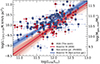 |
Fig. 4. CO luminosity vs. FIR luminosity bisector fits of AGN host galaxies (red circles) and non-active galaxies of their control sample (blue squares). The thick lines mark the bisector fits obtained by adopting a Bayesian framework (see main text). The dispersion of the fits is given by plotting 500 realizations of the bisector fits. The vertical axis on the right is derived by assuming αCO = 3.6 M⊙/(K km s−1 pc2) and serves for illustration purposes only, since we only consider L′CO in our quantitative analysis (see Sect. 5.1). |
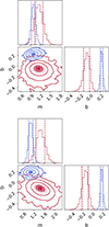 |
Fig. 5. Corner plots of best-fit parameters for the log( |

5.2. Molecular gas fraction distribution
We compared the molecular gas fraction distribution of AGN and control samples, measured as the observational proxy L′CO/M*, to further test the difference between AGN hosts and non-active galaxies. Similarly to C21, we do not address the distribution of the ratio of L′CO and LFIR (observational proxy for the SF depletion time) since around half of KASHz and SUPER targets present an upper limit in at least one of the two quantities, and a quarter of them show an upper limit for both. Our aim is to derive the total gas fraction distribution and mean value (μfgas) for the AGN and non-active galaxy samples to quantify how they relate to one another. Once more, we carry out our analysis in a Bayesian framework, which allows us to obtain posteriors for the mean of the distribution, by folding in the information contained on upper limits. We exclude three KASHz and SUPER AGN (cid_178, cid_1605, cid_467) because they have an upper limit for both L′CO and M*.
Following C21 (and Mullaney et al. 2015; Scholtz et al. 2018), we assumed that the distribution of molecular gas fraction of AGN and non-active galaxies follows a Gaussian distribution, supported by the tests performed by C21 to demonstrate the validity of such an assumption both on the xCOLD-GASS reference survey (Saintonge et al. 2017) and in PHIBSS galaxies at cosmic noon. We thus adopt their Bayesian hierarchical method: we assumed that the prior distribution, common to both samples, is Gaussian and defined by two hyper-parameters, that is, the mean μfgas and the standard deviation σfgas, for both of which we set uniform priors. Following the approach described in Sect. 5.1, we built the likelihood assuming Gaussian-distributed uncertainties for constrained gas fractions and error functions for the upper and lower limits. The total posterior distributions of the gas fractions of AGN hosts and non-active galaxies (red and blue histograms, respectively; see Fig. 6) were built by joining the sampled posterior distribution of each respective target and, as such, cover the full range of fgas spanned by each target with the advantage of carrying the information on how upper and lower limits are weighted by the prior Gaussian distribution. The same figure also shows the sampled posterior distribution of the mean of the hierarchical Gaussian prior that we obtained from our Bayesian analysis (red and blue violin plots, bottom panels). For the other quantities, we consider the 50th percentile as the best value and the 16th and 84th percentiles as uncertainties. We find that the mean log(L′CO/M*) of both our AGN samples is lower than that of non-active galaxies (see diamond-shaped markers in the bottom panel of Fig. 6), as also found by C21 for the sole SUPER sample.
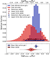 |
Fig. 6. Distribution of L′CO/M* (observational proxy of the gas fraction fgas) for AGN host galaxies (red) and non-active galaxies of the control sample (blue). Upper panel: filled histograms show the total distributions, obtained by joining the sampled posterior distribution of each target for both samples. The blue squares indicate the measure of each non-active galaxy (98 targets), red circles that of each AGN (40 targets). The blue and red triangles indicate upper limits if pointing leftward and lower limits if pointing rightward for the gas fraction of non-active galaxies and AGN, respectively. Lower panel: violin plots show the sampled posterior distribution of the mean of the hierarchical Gaussian prior used in our Bayesian analysis. The diamonds show the measured mean value μfgas of AGN (red) and non-active galaxies (blue). The top axis is derived by assuming αCO = 3.6 M⊙/(K km s−1 pc2) and serves for illustration purposes only since we only consider L′CO in our quantitative analysis (see Sect. 5.2). |
The mean gas fractions of AGN sample and control sample are different at the 2σ level (i.e., comparable to the 2.2σ result of C21) when considering only SUPER AGN. However, the total fgas distributions of AGN and non-active galaxies are significantly different according to the KS test (p-value < 10−7), and evidently skewed at low molecular gas fractions (see Fig. 6, upper panel).
5.3. Molecular gas mass and gas fraction versus stellar mass
We compared the molecular gas mass and gas fraction of AGN and non-active galaxies as a function of stellar mass through bisector fits, as described in Sect. 5.1. The best-fit parameters are summarized in Table 2. As in the previous section, we discard three KASHz and SUPER AGN (cid_178, cid_1605, cid_467) for the log(L′CO/M*) versus log M* case since they have upper limits in both stellar mass and CO emission.
The bisector best fits of AGN hosts and non-active galaxies both in the log L′CO versus log M* plane (see Fig. 7) and in the log(L′CO/M*) versus log M* plane (i.e., fgas vs. log M*) (see Fig. 8) are different at the ≲2σ level. This result holds in both parameter spaces also when excluding non-active galaxies and AGN hosts without a proper match in the other sample (see Sect. 3), and also when the samples include only targets on the MS (|ΔMS| ≃ 0.3 dex; 14 AGN, of which 8 have upper limits on L′CO, and 50 galaxies). Focusing on the y versus x Bayesian fits (i.e., considering uncertainties and upper limits on L′CO), the differences with non-active galaxies increase slightly (≃2σ), both for the full and the reduced samples (better match; only MS targets). Thus, we find a ≲2σ difference in molecular content and gas fraction between AGN and host galaxies for fixed stellar mass.
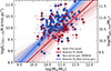 |
Fig. 7. CO luminosity vs. stellar mass bisector fits of AGN host galaxies (red circles) and non-active galaxies of the control sample (blue squares). The thick lines mark the bisector fits obtained by adopting a Bayesian framework (see main text). The dispersion of the fits is given by plotting 500 realizations of the bisector fits. The vertical axis on the right is derived by assuming αCO = 3.6 M⊙/(K km s−1 pc2) and serves for illustration purposes only since we only consider L′CO in our quantitative analysis (see Sect. 5.3). |
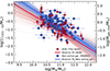 |
Fig. 8. Gas fraction vs. stellar mass bisector fits of AGN host galaxies (red circles) and non-active galaxies of the control sample (blue squares). The thick lines mark the bisector fits obtained by adopting a Bayesian framework (see main text). The dispersion of the fits is given by plotting 500 realizations of the bisector fits. The vertical axis on the right is derived by assuming |

5.4. Summary
For this section we compared the properties of AGN hosts and non-active galaxies in the following parameter spaces, finding the following differences:
-
L′CO(1 − 0) versus LFIR, where AGN and non-active galaxies are different at the 3σ level (see Sect. 5.1 and Figs. 4–5);
-
log(L′CO/M*) distribution (proxy of molecular gas fraction), where AGN and non-active galaxies show significantly different total distributions according to the KS test (p-value < 10−7); mean values consistent at the 2σ level; and consistent posterior distributions of the mean values (see violin plots in Fig. 6), indicating that the significant difference in the total distributions is driven by the skewness to lower values of the AGN distribution (see Sect. 5.2 and upper panel of Fig. 6);
-
L′CO(1 − 0) versus M* and log(L′CO/M*) versus M*, in both of which AGN and non-active galaxies are different at the ≲2σ (see Sect. 5.3 and Figs. 7–8).
The results obtained by excluding those AGN without a match in the control sample (i.e., galaxies well below the main sequence, ΔMS < −0.5 dex, at z = 1.8 − 2.6) are consistent with those summarized here. Thus, CO depletion at fixed FIR luminosity and different molecular gas fraction distributions, with AGN skewed at lower values, are indicative of an intrinsic difference between the total molecular gas content of AGN hosts and non-active galaxies and are not induced by biases in the control sample matching. Moreover, such a tail in the molecular gas fraction of the AGN sample without a correspondence in the non-active galaxies is also present when considering only SUPER AGN, as presented in C21 (see their Fig. 4). We note that AGN host galaxies present a trend of molecular gas fraction versus stellar mass similar to that of non-active galaxies, with decreasing gas fraction for increasing stellar mass, which resembles the mean general trend of star-forming galaxies (see, e.g., Tacconi et al. 2020; Saintonge & Catinella 2022, for a review). The reduced differences (≃2σ) in L′CO and fgas between AGN and non-active galaxies for fixed stellar mass could be due to the large error bars on the best-fit parameters, the large fraction of upper limits on the AGN side, and to the distribution of CO upper limits. There is no preferential locus for CO upper limits (see Figs. 7 and 8) for fixed stellar mass, while CO upper limits and CO detection are quite segregated, with CO upper limits (detections) mostly located at the lower (upper) end of the LFIR distribution (see Fig. 4), contributing to increasing the CO depletion effect. This is true also when restricting the AGN sample to host galaxies within 0.3dex distance from the MS.
Lastly, we note that the CO SLEDs assumed for AGN hosts and non-active galaxies are consistent with each other, and thus the reduced CO luminosity of AGN hosts is not a by-product of the assumed CO SLED. This is a conservative assumption since, despite the large uncertainties, AGN are seen to show higher CO(J → J − 1)/CO(1 − 0) ratios even at J < 5 (e.g., Kirkpatrick et al. 2019). Moreover, AGN hosts and non-active galaxies span the same range of CO flux at fixed J and similarly cover the same L′CO luminosity range, and thus there is no bias between the two samples in this sense.
6. Comparison with cosmological simulations
Ward et al. (2022) recently analyzed the output of three cosmological simulations (TNG, Springel et al. 2018; Pillepich et al. 2018; Naiman et al. 2018; Nelson et al. 2018; Marinacci et al. 2018, data release: Nelson et al. 2019; EAGLE, Crain et al. 2015; Schaye et al. 2015, data release: McAlpine et al. 2016; and SIMBA, Davé et al. 2019) with approaches similar to those taken by observers, to assess the predictions regarding the effects of AGN feedback on the properties of AGN host galaxies and how these relate with observational constraints and results. Ward et al. interestingly found that the simulations predict that powerful AGN tend to be located in gas-rich galaxies and that the gas-depleted fraction of AGN hosts is lower than that of non-active galaxies.
The molecular gas phase cannot be directly traced in cosmological simulations because, due to computational limitations, the ISM is poorly resolved. However, the amount of molecular hydrogen can be measured through models that are calibrated in the post-processing phase (e.g., Lagos et al. 2015; Diemer et al. 2018, 2019; Davé et al. 2019, using for instance the models by Gnedin & Kravtsov 2011). When tested against observational data, these models are in good agreement with the galaxy populations observed in the local Universe (Lagos et al. 2015; Diemer et al. 2019), while they slightly underestimate the amount of molecular gas observed at z ≃ 2 (by a factor of 1.5 in EAGLE, Lagos et al. 2015, and by a factor of 2–3 in TNG, Popping et al. 2019).
Following Ward et al. (2022), we compare the predictions for the molecular gas fraction of galaxies at cosmic noon of TNG, EAGLE, and SIMBA tuned to the observed range of M*, SFR, and Lbol spanned by our sample. We thus filter the simulations’ outputs at z = 2 to select galaxies with stellar masses higher than 1010 M⊙ and lower than 1011.7 M⊙ and log(SFR/M⊙ yr−1) within 0.7 and 2.8 (the lower and upper bounds of the observed sample; see Fig. 2). We then identify AGN hosts in the simulations by combining bolometric luminosity and Eddington ratio (λEdd) selection criteria. We use log Lbol > 44.3 erg s−1 to span the same bolometric luminosity range as our observations, and we also consider λEdd > 1% to remove those AGN accreting in a radiatively inefficient fashion. We identify non-active galaxies in the simulations as those systems with λEdd < 0.1%, yet we note that results are identical when the selection is relaxed (λEdd < 1%). Similarly to the analysis of Sect. 5.2, we remove from the observed sample the three AGN (cid_178, cid_1605, cid_467) for which both stellar mass and CO luminosity are upper limits.
Simulations only allow us to compute the molecular gas fraction as fH2 = MH2/M*, and thus we have to assume an αCO value to convert the observed fgas in fH2 = αCOfgas. One of the backbones of our work is not to select a value of αCO since it is nontrivial to discriminate whether each galaxy is more MS-like (αCO ≃ 3.6 M⊙ (K km s−1 pc2)−1; e.g., Daddi et al. 2010a; Genzel et al. 2015), more starburst-like (αCO = 0.8 M⊙ (K km s−1 pc2)−1; e.g., Downes & Solomon 1998; Solomon & Vanden Bout 2005; Calistro Rivera et al. 2018; Amvrosiadis et al. 2023) or somewhere in the middle (αCO = 1.8 − 2.5 M⊙ (K km s−1 pc2)−1, Cicone et al. 2018; Herrero-Illana et al. 2019; Montoya Arroyave et al. 2023). However, a good fraction of the AGN sample corresponds to MS host galaxies (see Fig. 2, thus we present the comparison between observed data and simulations assuming αCO = 3.6 M⊙ (K km s−1 pc2)−1 and show the shift corresponding to the lowest αCO value (αCO = 0.8 M⊙ (K km s−1 pc2)−1) in the plots.
Figure 9 shows the fH2 versus Lbol distribution of AGN in the simulations and in our observed sample. Density contours show the distribution of the simulated sources in TNG (red), EAGLE (purple), and SIMBA (orange), while the observed targets are shown as gray pentagons for ALMA KASHz AGN (presented in this work) and gray circles for SUPER AGN from C21 and this work. Figure 10 shows the comparison of simulations and observations in the fH2 versus SFR plane. We show AGN and non-active galaxies of the simulations computing their median molecular gas fraction in SFR bins of 0.3 dex width, and use the 18th and 64th percentiles as error bars. We also show the unbinned distribution of AGN host galaxies as hexagons, color-coded based on the mean stellar mass of the galaxies in each bin. Figure 11 compares the gas fraction distributions (violin plots) and mean values (diamonds) of AGN hosts and non-active galaxies from cosmological simulations and the total gas fraction distributions and mean values of observed AGN and non-active galaxies as derived in Sect. 5.2.
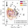 |
Fig. 9. Distribution of gas fraction fH2 vs. bolometric luminosity Lbol. Galaxies in the simulations are selected to match the observed parameter range in stellar mass and SFR, and to host AGN with Lbol > 1044.3 erg s−1 and λEdd > 0.01. Contours contain 90% of the selected systems and extreme outliers are shown as individual points. The color-coding for the simulations is as follows: EAGLE, TNG, and SIMBA in purple, red, and orange, respectively. Observational points are shown as gray pentagons for KASHz AGN (presented in this work) and gray circles for SUPER AGN from C21, scaled by αCO = 3.6 M⊙ (K km s−1 pc2)−1. The black arrow marks the downward shift for αCO = 0.8 M⊙ (K km s−1 pc2)−1. The bottom left point shows the mean error bar of the observational sample. |
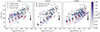 |
Fig. 10. Comparison of molecular gas fraction against SFR of AGN (red) and non-active galaxies (blue) from observations and simulations. SUPER ALMA targets are shown as red circles, KASHz AGN as red pentagons, and observed non-active galaxies as blue squares. Blue downward triangles and red upward triangles show the median and 16th–84th percentiles of non-active galaxies and AGN in the simulations, respectively, grouped in SFR bins of 0.3 dex. Hexagons show the distribution of simulated AGN and are color-coded based on the mean stellar mass of the host galaxies in each bin. Observed molecular gas fractions are computed assuming αCO = 3.6 M⊙ (K km s−1 pc2)−1. Galaxies in the simulations are filtered to match the observed properties of the observed galaxies. The black arrow marks the downward shift for αCO = 0.8 M⊙ (K km s−1 pc2)−1. |
While the KASHz survey in theory spans a very broad range of X-ray and bolometric luminosity (log(LX/erg s−1) = 41 − 45.3; log(Lbol/erg s−1)≃42 − 47 using the bolometric correction of Duras et al. 2020), the ALMA KASHz AGN have bolometric luminosity log(Lbol/erg s−1)≥44.3, comparable to the lower bound of the observed AGN used in Ward et al. (2022). As a consequence, despite the better sampling of the intermediate-luminosity regime, the Lbol range spanned by observed and simulated AGN in Fig. 9 hardly overlap, as seen by Ward et al. (2022). To bridge such a gap, both observations and simulations need to take a leap forward. On the one hand, we need to gather the observational information of AGN with lower bolometric luminosity, possibly through targeted programs. On the other hand, simulations still struggle to reproduce the high-Lbol population of AGN (Fig. 9), due to their small box size, which prevents them from reproducing rare and short-lived objects like AGN with Lbol > 1046 erg s−1. We note that this mismatch in Lbol is still present even by relaxing the SFR and M* filtering, as seen in Ward et al. (2022).
Additionally, cosmological simulations suggest that AGN hosts should match or exceed non-active galaxies in gas fraction, which is the opposite of the observed trend (see Fig. 11). We note that this result still holds, even when relaxing the mass and SFR filtering of the simulations’ outputs, as can be seen in the left column panels of Fig. 7 in Ward et al. (2022). EAGLE and Simba also suggest that AGN host galaxies show similar molecular gas masses for fixed SFR compared to non-active galaxies (see Fig. 10), which is at odds with our result in Sect. 5.1. However, AGN hosts in TNG show molecular gas depletion for fixed SFR, although with an opposite trend compared to the observations: the discrepancy increases for increasing SFR in the simulations, while in the observations it increases for decreasing SFR (see Fig. 4). Figure 10 also shows that simulations do not fully reproduce the observed properties of AGN host galaxies. SIMBA is the only cosmological simulation that covers the full M* and SFR range, while TNG and EAGLE are basically missing AGN hosts with M* > 1011 M⊙ and log(SFR/ M⊙ yr−1)≳2. However, a direct comparison to the simulations is difficult, as their limited box sizes and subgrid models for AGN feedback and molecular gas estimation reduce the overlap with our observations, especially at the high-mass, high-Lbol end.
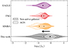 |
Fig. 11. Gas fraction distributions of AGN host galaxies (filled violin plots) and non-active galaxies (hatched violin plots) from cosmological simulations (EAGLE, TNG, and SIMBA in purple, red, and orange, respectively) and observations presented in this work (gray), scaled for αCO = 3.6 M⊙ (K km s−1 pc2)−1. The diamond markers give the mean value of each distribution. Gas fraction distributions from the observations correspond to the total gas fraction distributions built in Sect. 5.2. Galaxies in the simulations are filtered as in Fig. 9. The black arrow marks the leftward shift of observed distributions (black) for αCO = 0.8 M⊙ (K km s−1 pc2)−1. |
Another pressing issue that arises from the comparisons in Figures 9–11 is related to the choice of αCO. On the one hand, the gas fraction distributions of AGN hosts in the simulations are in fair agreement with the observed distributions of KASHz and SUPER AGN in the case of αCO = 3.6 M⊙ (K km s−1 pc2)−1 (see Fig. 11), in the sense that their mean values are consistent, but simulations seem to lack more gas-rich systems, which is evident also as a function of bolometric luminosity in Fig. 9. On the other hand, simulations fail to reproduce the observed fH2 distributions in the case of αCO = 0.8 M⊙ (K km s−1 pc2)−1 (see Fig. 11), but at the same time would show a better agreement with the observed fH2 versus Lbol distribution (see Fig. 9), at least in the range of Lbol, M*, and SFR used to filter the simulations’ outputs. The clear impact of the adopted value of αCO on the observed results in Figs. 11 and 9 further emphasizes the importance of measuring tracers that can be used to derive or set a prior for αCO, for instance metallicity and distance from the MS (e.g., Elbaz et al. 2007; Noeske et al. 2007; Accurso et al. 2017), two quantities that are not available for the full sample of AGN used in this work.
7. Discussion
Our results show that AGN at z = 1 − 2.6, uniformly selected and analyzed, without prior knowledge on feedback tracers (e.g., ionized outflows or radio jets), and non-active galaxies, matched in z, M*, SFR, are statistically different in terms of L′CO(1 − 0) versus LFIR (3σ level; see Sect. 5.1), and log(L′CO/M*) distribution (proxy of the molecular gas fraction distribution; p-value < 10−7; see Sect. 5.2). However, although there are hints of gas depletion even at fixed stellar mass (see Figs. 7–8), AGN and non-active galaxies are statistically consistent in the L′CO(1 − 0) versus M*, fgas versus M*, and log(L′CO/M*) versus M* two-dimensional spaces (see Sect. 5.3).
The control sample of non-active galaxies is built to match the properties shown by AGN host galaxies, and thus in principle the sample of selected non-active galaxies is an analog of our AGN hosts, the only difference being that they do not host an AGN. Moreover, we robustly controlled for consistency in SFR and M* between the two samples (see Sect. 3) and that our results remain unvaried when considering a subsample of AGN and non-active galaxies. Additionally, we trace the SF level in our galaxies through LFIR (i.e., corresponding to SF averaged over 100 Myr). Thus, we interpret our comparisons of AGN hosts and non-active galaxies in terms of differences (or absence thereof) in the molecular gas content due to the presence of the AGN.
In particular, we find that AGN hosts are, on average, more CO depleted for fixed FIR luminosity (see Fig. 4). In other words, AGN hosts show a reduced amount of cold molecular gas compared to matched non-active galaxies, and such reduced CO luminosities may lead to reduced SF in AGN hosts in the future. We note that this difference holds, even when we exclude AGN and non-active galaxies that are not well matched, and thus it does not depend on biases in building the control sample. Moreover, CO depletion is differential in LFIR, meaning that it increases for decreasing LFIR. CO content and molecular gas fraction for fixed stellar mass of AGN and non-active galaxies are different at the 2σ level (see Figs. 7–8). Such a reduced difference for fixed stellar mass could be driven by the differential CO depletion level for fixed SFR (see Fig. 4): at fixed stellar mass we are sampling galaxies that span a broad range of SF levels, which differentially depend on stellar mass (see, e.g., Fig. 8 of Saintonge & Catinella 2022). In this sense, the mixing of host galaxies with different SF levels and the differential CO depletion observed for fixed LFIR (see Fig. 4) likely dilute the differences between AGN and non-active galaxies for fixed stellar mass, and yet we do not find more enhanced differences considering only targets on the MS, possibly due to the small sample size (14 AGN host galaxies on the MS). Differences in the one-dimensional distributions of fgas are more prominent because the contribution of CO detections and upper limits in the AGN sample is better decoupled: the mean value of the distribution is mainly driven by CO detections, while CO upper limits (and in this case, fgas upper limits) shape the left wing of the distribution, producing the skewness at lower values that is missing in the distribution of non-active galaxies.
We confirm the hints observed by C21 in SUPER ALMA AGN, using a uniformly selected and homogeneously analyzed AGN sample that is twice as large: molecular gas depletion is significant also when considering moderate-luminosity AGN (44 ≲ log(Lbol/erg s−1)≲47). This work thus supports the scenario for which AGN play a key role in shaping the life of galaxies, in particular by altering the molecular gas reservoir of their hosts, as was observed in higher-Lbol sources (46 ≲ log(Lbol/erg s−1)≲48; e.g., Harrison et al. 2012; Brusa et al. 2018; Vietri et al. 2018; Perna et al. 2018; Bischetti et al. 2021). This is also coherent with the recent results in Frias Castillo et al. (2024) in moderate-luminosity lensed AGN (43 ≲ log(Lbol/erg s−1)≲46) at the end of cosmic noon (z = 1.2 − 1.6), which are seen as CO depleted for fixed FIR luminosity compared to star-forming galaxies. We also investigated the possibility of a dependency of the molecular gas fraction with properties of the AGN, such as the bolometric luminosity, but found no significant correlation, as already seen in previous studies (e.g., Shangguan et al. 2020b; C21).
In this work we assumed a CO SLED at J < 5 for AGN hosts that is consistent with that of non-active galaxies. This is a conservative assumption: works focused on determining the CO ladder of AGN found them to show higher rJ, 1 values compared to non-active galaxies, even at J < 5, despite the large error bars (e.g., Kirkpatrick et al. 2019; Boogaard et al. 2020). Moreover, the backbone of our analysis, and other previous studies, is to compare the gas content of AGN host galaxies and non-active galaxies in terms of L′CO, thus without assuming an αCO value. In this way the difference found between the two samples in molecular gas mass and fraction represents a lower limit of the real discrepancy. This would be unchanged if we were to assume the same αCO value for both AGN hosts and non-active galaxies, while the difference would increase in the case of the reasonable assumption of AGN hosts showing lower αCO values than non-active galaxies (see, e.g., Bolatto et al. 2013, and references therein). Given all our conservative assumptions, our results indeed provide evidence that AGN reduce the molecular gas reservoir of their hosts, and thus impact on their evolution.
Bischetti et al. (2021) recently investigated the effects of AGN feedback on the molecular gas reservoir of WISSH quasars. Among the various tests, the authors compared the gas fraction of WISSH AGN with that of star-forming galaxies after correcting for the evolution of the gas fractions with redshift and distance from the MS (ΔMS = sSFR/sSFRMS). Analyses focused on assessing the molecular gas content of star-forming galaxies up to z ≃ 4 (e.g., Genzel et al. 2015; Tacconi et al. 2018) pointed out a dependency of the gas fraction on redshift and distance from the MS. Our analysis already accounts for the redshift evolution of the MS when building the control sample by matching AGN and galaxies in two redshift bins (z ≃ 1 − 1.8, z ≃ 2 − 2.6), within which the MS evolution is not large (≃0.2 dex; e.g., Whitaker et al. 2012). However, not correcting for the distance from the MS could still affect the comparison of non-active galaxies and AGN hosts. Unfortunately, such a correction is not viable for the AGN sample used in this work: about half of our targets have upper limits on LFIR, making it impossible to constrain how much they deviate from the MS. Nonetheless, we tentatively measure the ΔMS = sSFR/sSFRMS parameter of the AGN sample considering LFIR at face value and compute the gas fractions corrected for the distance from the MS ( ) using Equation (15) of Genzel et al. (2015) in which sSFRMS is parameterized as in Whitaker et al. (2012). We conservatively assume αCO = 3.6 M⊙ (K km s−1 pc2)−1 for both AGN and non-active galaxies. Applying the analysis of Sect. 5.2, we find that the
  total distributions of AGN and non-active galaxies are still significantly different according to the KS test (p value < 0.001), with consistent mean values, both using the full sample and excluding those AGN and non-active galaxies without a good match (see Sect. 3). Following the analysis of Sect. 5.3, we also find that AGN and non-active galaxies are consistent with each other within 2σ in the
  versus M* parameter space.
There are still some effects that we are not fully considering, or cannot fully consider, when studying AGN feedback. First, we are comparing two phenomena that occur on very different timescales (e.g., Harrison 2017; Harrison et al. 2018; Harrison & Ramos Almeida 2024): the timescales of visible AGN activity do not necessarily mirror the AGN duty cycle, plus the timescales of feeding and feedback in general are uncertain. For instance, the AGN might have become less luminous or non-visible by the time the effects of its impact have become observable, or even the galaxy might have accreted more gas from its surroundings (e.g., from the CGM) reducing the overall depletion effect of AGN activity. Additionally, we have no means of understanding how long the currently observed AGN has been active or if it is the n-th active phase in a cycle of flickering accretion. In other words, we cannot know how much energy the AGN has input in the surrounding medium before being observed, and thus on the total energy input in the system on timescales that are relevant for SF activity.
Second, we are comparing phenomena and effects happening on spatial scales that are possibly very different: high-resolution studies in the local Universe revealed AGN that create regions of CO depletion in their surroundings (within the central few 100 pc to kpc; e.g., Sabatini et al. 2018; Rosario et al. 2019; Fluetsch et al. 2019; Feruglio et al. 2020; Ellison et al. 2021), where the bulk of the molecular gas is possibly in a warmer phase due to AGN heating (e.g., through accretion radiation in the form of X-ray photons, Fabbiano et al. 2019). Studies regarding SF activity in local AGN confirm such a scenario where AGN have a significant impact only in their surroundings, either reducing (e.g., García-Burillo et al. 2021, 2024; Molina et al. 2023) or enhancing (e.g., Cresci et al. 2015; Lammers et al. 2023) the central SF without affecting it on larger scales. However, this work supports the scenario in which AGN at cosmic noon are indeed affecting the total molecular gas mass of galaxies (e.g., total molecular gas mass, future total SFR), and thus a significant portion of the full system. An additional possibility is that AGN excite CO higher up in the rotational ladder without making the host molecular gas poor (e.g., Paraficz et al. 2018; Fogasy et al. 2020; Spingola et al. 2020). However, such a scenario cannot be probed with the present sample since many AGN were targeted in only one CO transition.
Third, the SUPER and KASHz surveys have selected AGN only based on their X-ray luminosity and redshift values, with no priors regarding AGN-driven outflows and AGN feedback effects. Here and in C21, we investigated AGN feedback by studying the overall properties of the AGN sample compared to those of non-active galaxies. Literature results finding AGN hosts to be significantly gas depleted, or with reduced depletion timescales, are usually associated with sources showing massive AGN-driven outflows on kiloparsec scales in at least one gas phase and that are often caught at the peak of their power (e.g., Carniani et al. 2017; Brusa et al. 2018; Loiacono et al. 2019, but see also Scholtz et al. 2021; Lamperti et al. 2021). One might then infer that gas depletion is significant and widespread only in those sources where feedback is caught in the act. However, gas depletion in AGN host galaxies could be also due to earlier AGN event(s), so that the reduction in gas content and/or SF activity is a product of the integrated past activity of the AGN (e.g., Piotrowska et al. 2022). A detailed comparison between [OIII] outflows and CO properties of KASHz and SUPER targets is beyond the scope of the present study and will be the subject of a future work.
Lastly, this work provides a sizeable, uniformly selected, and uniformly analyzed sample to compare observations and predictions of cosmological simulations. We compared the observed cosmic noon AGN and sample of non-active galaxies with the properties of AGN and galaxies from three cosmological simulations (TNG, EAGLE, and SIMBA, following Ward et al. 2022), by filtering their outputs at z = 2 to match the properties of the observed sample of AGN (see Sect. 6). One of the issues encountered in Ward et al. (2022), and also in this work (see Fig. 9), is that simulations and data hardly overlap, especially in terms of bolometric luminosity. Our observed sample provides better coverage of the 44 < log(Lbol/erg s−1) < 46 than previously available. However, a robust sampling of observed AGN at log(Lbol/erg s−1) < 44, where the bulk of simulated AGN lies, is still lacking. Moreover, the three simulations predict that AGN hosts should match non-active galaxies in molecular gas mass for fixed SFR (see Fig. 10) and that they should even exceed non-active galaxies in gas fraction (see Fig. 11). The only exception is TNG, which predicts that AGN are gas depleted for fixed SFR, but with a trend (increasing gas depletion for increasing SFR) that is opposite to what seen in the observations (see Fig. 4). Another issue encountered in these comparisons is that only SIMBA covers the full parameter range of observed AGN hosts, while TNG and EAGLE are missing AGN hosts with M* > 1011 M⊙ and  . Lastly, we also highlight another well-known issue: the selection of the “right” αCO value. How well (or not well) the simulations agree with the observed properties strongly depends on the chosen value for αCO (see Sect. 6 and Figs. 9–11). For the present sample, for instance, additional observations for measuring the metallicity and better constraining the distance from the MS could allow us to take advantage of the continuous αCO(z, ΔMS) function of Accurso et al. (2017) and solve this issue.
8. Summary and conclusions
This work addresses the effects of AGN activity on the molecular gas content of host galaxies with a carefully selected, sizable sample of AGN at cosmic noon, to shed light on whether AGN have any impact on the fuel of future star formation.
-
We collected all the available ALMA observations of CO (J < 5) emission lines of KASHz AGN at cosmic noon, a survey built to study AGN feedback in X-ray-selected AGN as traced by the ionized gas component. We complemented our KASHz ALMA sample with SUPER ALMA targets from C21 (observed in CO(3–2)). Being heterogeneous in the CO transitions observed (CO(2–1), CO(3–2), CO(4–3)), we assumed a reasonable CO excitation ladder (from Kirkpatrick et al. 2019) to convert our measurements to the CO(1–0). Other key quantities of the AGN+galaxy system were retrieved through SED fitting with the CIGALE code (Boquien et al. 2019; Yang et al. 2020), collecting the most up-to-date multiwavelength broadband photometry, as provided by the deep-field survey collaborations (CANDELS/GOODS-S, COSMOS, HELP collaboration).
-
The AGN sample thus totals 46 AGN at z = 1 − 2.6 i.e., a sample size that is twice that of the SUPER AGN presented in C21 and with a larger CO detection rate (≃50% vs. 40%). We built the control sample of non-active galaxies (98 galaxies), matched in z, M*, and SFR to our AGN sample, by capitalizing on the PHIBSS project (Tacconi et al. 2018, and references therein), on the ASPECS survey (Boogaard et al. 2020, and references therein), and on the ALMA/NOEMA survey of sub-mm galaxies in the COSMOS, UDS, and ECDFS fields by Birkin et al. (2021).
-
We then quantitatively compared AGN and non-active galaxies in a Bayesian framework, as developed by C21, robustly considering upper and lower limits in any of the considered quantities. The samples were compared in terms of i)L′CO(1 − 0) versus LFIR (see Sect. 5.1), ii) log(L′CO/M*) distribution (proxy of the gas fraction distribution; see Sect. 5.2), iii)L′CO(1 − 0) versus M*, and iv) log(L′CO/M*) versus M* (see Sect. 5.3). Our results confirm the hints observed by C21 on SUPER AGN: AGN hosts at cosmic noon, selected without priors regarding AGN feedback, are significantly gas depleted compared to non-active galaxies. Differences in the log(L′CO/M*) versus M* and L′CO(1 − 0) vs. M* two-dimensional spaces are possibly washed out by the rather uniform distribution of CO upper limits with respect to stellar mass (see Figs. 7–8), and the differential CO depletion observed for fixed LFIR (see Fig. 4).
-
Building on the study of Ward et al. (2022), we also compared our observed samples of AGN and non-active galaxies with the output of three cosmological simulations (TNG, EAGLE, SIMBA), filtered to match the properties of the observed AGN, AGN hosts and non-active galaxies (see Sect. 6). We find that SIMBA is the only simulation that can closely reproduce the mass and SFR of host galaxies; that TNG is the only simulation predicting gas depletion for fixed SFR in AGN hosts, but with a trend opposite to that of observations (see Fig. 10); and that all three equally fail at reproducing the observed distribution of molecular gas fractions (see Fig. 11) and bolometric luminosity (see Fig. 9).
The latest (and upcoming) facilities have opened (and will broaden) new windows to assess AGN feedback in the high-z Universe, especially regarding high spatial resolution studies. ALMA has proven its outstanding capabilities over the past decade, but high-resolution observations, matching the spatial resolution of NIR data, are still highly time-consuming, yet necessary to fully understand how AGN affect the molecular gas distribution within their hosts and bridge the gap between the local Universe and cosmic noon. Nonetheless, JWST/MIRI will allow us to probe molecular transitions previously inaccessible at cosmic noon, like the roto-vibrational H2 lines, which can shed new light on the effects of AGN activity on the molecular gas phase. Three SUPER targets (one of which is shared with KASHz), selected based on their prominent [O III] outflows, will be observed by JWST/MIRI/MRS (PI: V. Mainieri; wavelength coverage: λ ≃ 6.5 − 27.9 μm) to map the warm-molecular gas phase, thus completing their multiphase characterization. We will be able to determine the dynamics of the molecular gas and to derive the total (ionized+molecular) mass outflow rate and kinetic energy for these outflows, some of the most difficult wind parameters to measure with accuracy, thus providing a key constraint for current models of AGN feedback (e.g., Costa et al. 2020).
Data availability
Tables E.1–E.3 are available at the CDS via anonymous ftp to cdsarc.cds.unistra.fr (130.79.128.5) or via https://cdsarc.cds.unistra.fr/viz-bin/cat/J/A+A/691/A178
Supplementary material is available at: https://doi.org/10.5281/zenodo.13149280
The parameter  ) corresponds to the slope of a nominal power-law connecting the rest-frame UV and X-ray emission of AGN (Tananbaum et al. 1979).
The HerMES data was accessed through the Herschel Database in Marseille (HeDaM 11 operated by CeSAM and hosted by the Laboratoire d’Astrophysique de Marseille.
Fig. D.1 shows the SED of lid_1639 as example. The SEDs of the rest of the AGN sample are available on Zenodo at the following link: https://doi.org/10.5281/zenodo.13149280.
Acknowledgments
EB thanks R. Decarli, L. Boogaard, G. Sabatini and L. Barchiesi for useful discussion. We acknowledge financial support from INAF under the Large Grant 2022 “The metal circle: a new sharp view of the baryon cycle up to Cosmic Dawn with the latest generation IFU facilities”, from ASI under grants ASI-INAF I/037/12/0 and n. 2017-14-H.O, and from the grant PRIN MIUR 2017PH3WAT (“Black hole winds and the baryon life cycle of galaxies”). MD and EB gratefully acknowledge INAF funding through the “Ricerca Fondamentale 2022” program (mini-grant 1.05.12.04.04). SRW acknowledges funding from the Deutsche Forschungsgemeinschaft (DFG, German Research Foundation) under Germany’s Excellence Strategy: EXC-2094-390783311. AF acknowledges the support from project “VLT-MOONS” CRAM 1.05.03.07. AP acknowledges support from Fondazione Cariplo grant no. 2020-0902. AM and MG acknowledge support from grant PRIN-MUR 2020ACSP5K_002 financed by European Union - Next Generation EU. IL acknowledges support from PID2022-140483NB-C22 funded by AEI 10.13039/501100011033 and BDC 20221289 funded by MCIU by the Recovery, Transformation and Resilience Plan from the Spanish State, and by NextGenerationEU from the European Union through the Recovery and Resilience Facility. MP acknowledges support from the research project PID2021-127718NB-I00 of the Spanish Ministry of Science and Innovation/State Agency of Research (MCIN/AEI/10.13039/501100011033). DMA thanks the Science Technology Facilities Council (STFC) for support from the Durham consolidated grant (ST/T000244/1). CC has received funding from the European Union’s Horizon 2020 research and innovation programme under grant agreement No 951815 (AtLAST). CH acknowledges funding from a United Kingdom Research and Innovation grant (code: MR/V022830/1). IEL received funding from the European Union’s Horizon 2020 research and innovation program under Marie Skłodowska-Curie grant agreement No. 860744 “Big Data Applications for Black Hole Evolution Studies” (BiD4BESt (https://www.bid4best.org/)). G.T. acknowledge financial support from the European Research Council (ERC) Advanced Grant under the European Union’s Horizon Europe research and innovation programme (grant agreement AdG GALPHYS, No. 101055023). This paper makes use of ALMA data as listed in Table C.1. ALMA is a partnership of the ESO (representing its member states), NSF (USA), and NINS (Japan), together with the NRC (Canada), NSC and ASIAA (Taiwan), and KASI (Republic of Korea), in cooperation with the Republic of Chile. The Joint ALMA Observatory is operated by the ESO, AUI/NRAO, and NAOJ. This paper is based on observations carried out with the IRAM Interferometer NOEMA. IRAM is supported by INSU/CNRS (France), MPG (Germany) and IGN (Spain). The project leading to this publication has received support from ORP, that is funded by the European Union’s Horizon 2020 research and innovation program under grant agreement No 101004719 [ORP]. This work made use of computing resources and technical support from INAF-OAS Bologna and the Italian node of the European ALMA Regional Center, hosted by INAF-Istituto di Radioastronomia. EB thanks M. Dadina for granting the use of sbuccia whenever needed. This research made use of the spectral-cube (https://github.com/radio-astro-tools/spectral-cube), numpy (Harris et al. 2020), astropy (Astropy Collaboration 2013, 2018) and scipy (Virtanen et al. 2020) Python packages. This research made use of data from HerMES project (http://hermes.sussex.ac.uk/). HerMES is a Herschel Key Programme utilising Guaranteed Time from the SPIRE instrument team, ESAC scientists and a mission scientist. The HerMES data was accessed through the Herschel Database in Marseille (HeDaM (http://hedam.lam.fr)) operated by CeSAM and hosted by the Laboratoire d’Astrophysique de Marseille.
References
- Accurso, G., Saintonge, A., Catinella, B., et al. 2017, MNRAS, 470, 4750 [NASA ADS] [Google Scholar]
- Aird, J., Coil, A. L., Georgakakis, A., et al. 2015, MNRAS, 451, 1892 [Google Scholar]
- Akiyama, M., Ueda, Y., Watson, M. G., et al. 2015, PASJ, 67, 82 [NASA ADS] [CrossRef] [Google Scholar]
- Alexander, D. M., & Hickox, R. C. 2012, New Astron. Rev., 56, 93 [Google Scholar]
- Almaini, O., Foucaud, S., Lane, K., et al. 2007, ASP Conf. Ser., 379, 163 [NASA ADS] [Google Scholar]
- Amvrosiadis, A., Wardlow, J. L., Birkin, J. E., et al. 2023, ArXiv e-prints [arXiv:2312.08959] [Google Scholar]
- Ananna, T. T., Salvato, M., LaMassa, S., et al. 2017, ApJ, 850, 66 [Google Scholar]
- Aravena, M., Decarli, R., Gónzalez-López, J., et al. 2019, ApJ, 882, 136 [Google Scholar]
- Aravena, M., Boogaard, L., Gónzalez-López, J., et al. 2020, ApJ, 901, 79 [NASA ADS] [CrossRef] [Google Scholar]
- Astropy Collaboration (Robitaille, T. P., et al.) 2013, A&A, 558, A33 [NASA ADS] [CrossRef] [EDP Sciences] [Google Scholar]
- Astropy Collaboration (Price-Whelan, A. M., et al.) 2018, AJ, 156, 123 [Google Scholar]
- Bessiere, P. S., & Ramos Almeida, C. 2022, MNRAS, 512, L54 [NASA ADS] [CrossRef] [Google Scholar]
- Birkin, J. E., Weiss, A., Wardlow, J. L., et al. 2021, MNRAS, 501, 3926 [Google Scholar]
- Bischetti, M., Piconcelli, E., Vietri, G., et al. 2017, A&A, 598, A122 [NASA ADS] [CrossRef] [EDP Sciences] [Google Scholar]
- Bischetti, M., Feruglio, C., Piconcelli, E., et al. 2021, A&A, 645, A33 [NASA ADS] [CrossRef] [EDP Sciences] [Google Scholar]
- Bolatto, A. D., Wolfire, M., & Leroy, A. K. 2013, ARA&A, 51, 207 [CrossRef] [Google Scholar]
- Boogaard, L. A., Decarli, R., González-López, J., et al. 2019, ApJ, 882, 140 [NASA ADS] [CrossRef] [Google Scholar]
- Boogaard, L. A., van der Werf, P., Weiss, A., et al. 2020, ApJ, 902, 109 [NASA ADS] [CrossRef] [Google Scholar]
- Boquien, M., Burgarella, D., Roehlly, Y., et al. 2019, A&A, 622, A103 [NASA ADS] [CrossRef] [EDP Sciences] [Google Scholar]
- Brusa, M., Perna, M., Cresci, G., et al. 2016, A&A, 588, A58 [NASA ADS] [CrossRef] [EDP Sciences] [Google Scholar]
- Brusa, M., Cresci, G., Daddi, E., et al. 2018, A&A, 612, A29 [NASA ADS] [CrossRef] [EDP Sciences] [Google Scholar]
- Bruzual, G., & Charlot, S. 2003, MNRAS, 344, 1000 [NASA ADS] [CrossRef] [Google Scholar]
- Buat, V., Mountrichas, G., Yang, G., et al. 2021, A&A, 654, A93 [NASA ADS] [CrossRef] [EDP Sciences] [Google Scholar]
- Calistro Rivera, G., Hodge, J. A., Smail, I., et al. 2018, ApJ, 863, 56 [Google Scholar]
- Calzetti, D., Armus, L., Bohlin, R. C., et al. 2000, ApJ, 533, 682 [NASA ADS] [CrossRef] [Google Scholar]
- Carilli, C. L., & Walter, F. 2013, ARA&A, 51, 105 [NASA ADS] [CrossRef] [Google Scholar]
- Carniani, S., Marconi, A., Maiolino, R., et al. 2017, A&A, 605, A105 [NASA ADS] [CrossRef] [EDP Sciences] [Google Scholar]
- CASA Team (Bean, B., et al.) 2022, PASP, 134, 114501 [NASA ADS] [CrossRef] [Google Scholar]
- Chabrier, G. 2003, ApJ, 586, L133 [NASA ADS] [CrossRef] [Google Scholar]
- Chen, C.-C., Hodge, J. A., Smail, I., et al. 2017, ApJ, 846, 108 [Google Scholar]
- Cicone, C., Severgnini, P., Papadopoulos, P. P., et al. 2018, ApJ, 863, 143 [NASA ADS] [CrossRef] [Google Scholar]
- Circosta, C., Mainieri, V., Padovani, P., et al. 2018, A&A, 620, A82 [EDP Sciences] [Google Scholar]
- Circosta, C., Mainieri, V., Lamperti, I., et al. 2021, A&A, 646, 96 [Google Scholar]
- Civano, F., Marchesi, S., Comastri, A., et al. 2016, ApJ, 819, 62 [Google Scholar]
- Costa, T., Rosdahl, J., Sijacki, D., & Haehnelt, M. G. 2018, MNRAS, 479, 2079 [Google Scholar]
- Costa, T., Pakmor, R., & Springel, V. 2020, MNRAS, 497, 5229 [Google Scholar]
- Crain, R. A., Schaye, J., Bower, R. G., et al. 2015, MNRAS, 450, 1937 [NASA ADS] [CrossRef] [Google Scholar]
- Cresci, G., Mainieri, V., Brusa, M., et al. 2015, ApJ, 799, 82 [Google Scholar]
- Cresci, G., Tozzi, G., Perna, M., et al. 2023, A&A, 672, A128 [NASA ADS] [CrossRef] [EDP Sciences] [Google Scholar]
- Daddi, E., Bournaud, F., Walter, F., et al. 2010a, ApJ, 713, 686 [NASA ADS] [CrossRef] [Google Scholar]
- Daddi, E., Elbaz, D., Walter, F., et al. 2010b, ApJ, 714, L118 [NASA ADS] [CrossRef] [Google Scholar]
- Dale, D. A., Helou, G., Magdis, G. E., et al. 2014, ApJ, 784, 83 [Google Scholar]
- D’Amato, Q., Gilli, R., Vignali, C., et al. 2020, A&A, 636, A37 [NASA ADS] [CrossRef] [EDP Sciences] [Google Scholar]
- Davé, R., Anglés-Alcázar, D., Narayanan, D., et al. 2019, MNRAS, 486, 2827 [Google Scholar]
- Decarli, R., Walter, F., Aravena, M., et al. 2016, ApJ, 833, 70 [NASA ADS] [CrossRef] [Google Scholar]
- Decarli, R., Walter, F., Gónzalez-López, J., et al. 2019, ApJ, 882, 138 [Google Scholar]
- Diemer, B., Stevens, A. R. H., Forbes, J. C., et al. 2018, ApJS, 238, 33 [NASA ADS] [CrossRef] [Google Scholar]
- Diemer, B., Stevens, A. R. H., Lagos, C. D. P., et al. 2019, MNRAS, 487, 1529 [Google Scholar]
- Downes, D., & Solomon, P. M. 1998, ApJ, 507, 615 [NASA ADS] [CrossRef] [Google Scholar]
- Duras, F., Bongiorno, A., Ricci, F., et al. 2020, A&A, 636, A73 [NASA ADS] [CrossRef] [EDP Sciences] [Google Scholar]
- Elbaz, D., Daddi, E., Le Borgne, D., et al. 2007, A&A, 468, 33 [NASA ADS] [CrossRef] [EDP Sciences] [Google Scholar]
- Ellison, S. L., Wong, T., Sánchez, S. F., et al. 2021, MNRAS, 505, L46 [NASA ADS] [CrossRef] [Google Scholar]
- Esposito, F., Vallini, L., Pozzi, F., et al. 2022, MNRAS, 512, 686 [NASA ADS] [CrossRef] [Google Scholar]
- Fabbiano, G., Paggi, A., & Elvis, M. 2019, ApJ, 876, L18 [NASA ADS] [CrossRef] [Google Scholar]
- Fabian, A. C. 2012, ARA&A, 50, 455 [Google Scholar]
- Feltre, A., Hatziminaoglou, E., Fritz, J., & Franceschini, A. 2012, MNRAS, 426, 120 [Google Scholar]
- Feruglio, C., Fabbiano, G., Bischetti, M., et al. 2020, ApJ, 890, 29 [Google Scholar]
- Fiore, F., Feruglio, C., Shankar, F., et al. 2017, A&A, 601, A143 [NASA ADS] [CrossRef] [EDP Sciences] [Google Scholar]
- Fluetsch, A., Maiolino, R., Carniani, S., et al. 2019, MNRAS, 483, 4586 [NASA ADS] [Google Scholar]
- Fogasy, J., Knudsen, K. K., Drouart, G., Lagos, C. D. P., & Fan, L. 2020, MNRAS, 493, 3744 [NASA ADS] [CrossRef] [Google Scholar]
- Foreman-Mackey, D., Hogg, D. W., Lang, D., & Goodman, J. 2013, PASP, 125, 306 [Google Scholar]
- Frias Castillo, M., Rybak, M., Hodge, J., et al. 2024, A&A, 683, A211 [NASA ADS] [CrossRef] [EDP Sciences] [Google Scholar]
- Fritz, J., Franceschini, A., & Hatziminaoglou, E. 2006, MNRAS, 366, 767 [Google Scholar]
- Furusawa, H., Kosugi, G., Akiyama, M., et al. 2008, ApJS, 176, 1 [NASA ADS] [CrossRef] [Google Scholar]
- García-Burillo, S., Alonso-Herrero, A., Ramos Almeida, C., et al. 2021, A&A, 652, A98 [NASA ADS] [CrossRef] [Google Scholar]
- García-Burillo, S., Hicks, E. K. S., Alonso-Herrero, A., et al. 2024, A&A, 689, A347 [NASA ADS] [CrossRef] [EDP Sciences] [Google Scholar]
- Genzel, R., Tacconi, L. J., Lutz, D., et al. 2015, ApJ, 800, 20 [Google Scholar]
- Gnedin, N. Y., & Kravtsov, A. V. 2011, ApJ, 728, 88 [NASA ADS] [CrossRef] [Google Scholar]
- González-López, J., Decarli, R., Pavesi, R., et al. 2019, ApJ, 882, 139 [Google Scholar]
- González-López, J., Novak, M., Decarli, R., et al. 2020, ApJ, 897, 91 [Google Scholar]
- Goodman, J., & Weare, J. 2010, Commun. Appl. Math. Comput. Sci., 5, 65 [Google Scholar]
- Harris, C. R., Millman, K. J., van der Walt, S. J., et al. 2020, Nature, 585, 357 [NASA ADS] [CrossRef] [Google Scholar]
- Harrison, C. M. 2017, Nat. Astron., 1, 0165 [NASA ADS] [CrossRef] [Google Scholar]
- Harrison, C. M., & Ramos Almeida, C. 2024, Galaxies, 12, 17 [NASA ADS] [CrossRef] [Google Scholar]
- Harrison, C. M., Alexander, D. M., Swinbank, A. M., et al. 2012, MNRAS, 426, 1073 [NASA ADS] [CrossRef] [Google Scholar]
- Harrison, C. M., Alexander, D. M., Mullaney, J. R., et al. 2016, MNRAS, 456, 1195 [Google Scholar]
- Harrison, C. M., Costa, T., Tadhunter, C. N., et al. 2018, Nat. Astron., 2, 198 [Google Scholar]
- Herrera-Camus, R., Tacconi, L., Genzel, R., et al. 2019, ApJ, 871, 37 [NASA ADS] [CrossRef] [Google Scholar]
- Herrero-Illana, R., Privon, G. C., Evans, A. S., et al. 2019, A&A, 628, A71 [EDP Sciences] [Google Scholar]
- Hodge, J. A., & da Cunha, E. 2020, Royal Soc. Open Sci., 7, 200556 [NASA ADS] [CrossRef] [Google Scholar]
- Hurley, P. D., Oliver, S., Betancourt, M., et al. 2017, MNRAS, 464, 885 [Google Scholar]
- Husemann, B., Davis, T. A., Jahnke, K., et al. 2017, MNRAS, 470, 1570 [NASA ADS] [CrossRef] [Google Scholar]
- Inoue, A. K. 2011, MNRAS, 415, 2920 [NASA ADS] [CrossRef] [Google Scholar]
- Isobe, T., Feigelson, E. D., Akritas, M. G., & Babu, G. J. 1990, ApJ, 364, 104 [Google Scholar]
- Jarvis, M. E., Harrison, C. M., Mainieri, V., et al. 2020, MNRAS, 498, 1560 [NASA ADS] [CrossRef] [Google Scholar]
- Jin, S., Daddi, E., Liu, D., et al. 2018, ApJ, 864, 56 [Google Scholar]
- Kakkad, D., Mainieri, V., Brusa, M., et al. 2017, MNRAS, 468, 4205 [Google Scholar]
- Kakkad, D., Mainieri, V., Vietri, G., et al. 2020, A&A, 642, A147 [NASA ADS] [CrossRef] [EDP Sciences] [Google Scholar]
- Kakkad, D., Mainieri, V., Vietri, G., et al. 2023, MNRAS, 520, 5783 [NASA ADS] [CrossRef] [Google Scholar]
- Kennicutt, R. C., Jr 1989, ApJ, 344, 685 [CrossRef] [Google Scholar]
- Kennicutt, R. C., Jr 1998, ApJ, 498, 541 [Google Scholar]
- Kirkpatrick, A., Sharon, C., Keller, E., & Pope, A. 2019, ApJ, 879, 41 [NASA ADS] [CrossRef] [Google Scholar]
- Kocevski, D. D., Hasinger, G., Brightman, M., et al. 2018, ApJS, 236, 48 [CrossRef] [Google Scholar]
- Kormendy, J., & Ho, L. C. 2013, ARA&A, 51, 511 [Google Scholar]
- Koss, M. J., Strittmatter, B., Lamperti, I., et al. 2021, ApJS, 252, 29 [CrossRef] [Google Scholar]
- Lagos, C. D. P., Crain, R. A., Schaye, J., et al. 2015, MNRAS, 452, 3815 [NASA ADS] [CrossRef] [Google Scholar]
- Laigle, C., McCracken, H. J., Ilbert, O., et al. 2016, ApJS, 224, 24 [Google Scholar]
- LaMassa, S. M., Urry, C. M., Cappelluti, N., et al. 2016, ApJ, 817, 172 [NASA ADS] [CrossRef] [Google Scholar]
- Lammers, C., Iyer, K. G., Ibarra-Medel, H., et al. 2023, ApJ, 953, 26 [NASA ADS] [CrossRef] [Google Scholar]
- Lamperti, I., Saintonge, A., De Looze, I., et al. 2019, MNRAS, 489, 4389 [Google Scholar]
- Lamperti, I., Harrison, C. M., Mainieri, V., et al. 2021, A&A, 654, A90 [NASA ADS] [CrossRef] [EDP Sciences] [Google Scholar]
- Lanzuisi, G., Civano, F., Elvis, M., et al. 2013, MNRAS, 431, 978 [NASA ADS] [CrossRef] [Google Scholar]
- Lanzuisi, G., Ranalli, P., Georgantopoulos, I., et al. 2015, A&A, 573, A137 [NASA ADS] [CrossRef] [EDP Sciences] [Google Scholar]
- Lapi, A., Raimundo, S., Aversa, R., et al. 2014, ApJ, 782, 69 [NASA ADS] [CrossRef] [Google Scholar]
- Lehmer, B. D., Alexander, D. M., Geach, J. E., et al. 2009, ApJ, 691, 687 [Google Scholar]
- Liu, T., Tozzi, P., Wang, J.-X., et al. 2017, ApJS, 232, 8 [NASA ADS] [CrossRef] [Google Scholar]
- Loiacono, F., Talia, M., Fraternali, F., et al. 2019, MNRAS, 489, 681 [Google Scholar]
- Luo, B., Brandt, W. N., Xue, Y. Q., et al. 2017, ApJS, 228, 2 [Google Scholar]
- Lusso, E., & Risaliti, G. 2016, ApJ, 819, 154 [Google Scholar]
- Lutz, D., Poglitsch, A., Altieri, B., et al. 2011, A&A, 532, A90 [NASA ADS] [CrossRef] [EDP Sciences] [Google Scholar]
- Madau, P., & Dickinson, M. 2014, ARA&A, 52, 415 [Google Scholar]
- Marchesi, S., Lanzuisi, G., Civano, F., et al. 2016, ApJ, 830, 100 [Google Scholar]
- Marinacci, F., Vogelsberger, M., Pakmor, R., et al. 2018, MNRAS, 480, 5113 [NASA ADS] [Google Scholar]
- Martocchia, S., Piconcelli, E., Zappacosta, L., et al. 2017, A&A, 608, A51 [NASA ADS] [CrossRef] [EDP Sciences] [Google Scholar]
- McAlpine, S., Helly, J. C., Schaller, M., et al. 2016, Astron. Comput., 15, 72 [NASA ADS] [CrossRef] [Google Scholar]
- McConnell, N. J., Ma, C.-P., Gebhardt, K., et al. 2011, Nature, 480, 215 [NASA ADS] [CrossRef] [Google Scholar]
- Merlin, E., Castellano, M., Santini, P., et al. 2021, A&A, 649, A22 [NASA ADS] [CrossRef] [EDP Sciences] [Google Scholar]
- Mingozzi, M., Vallini, L., Pozzi, F., et al. 2018, MNRAS, 474, 3640 [NASA ADS] [CrossRef] [Google Scholar]
- Molina, J., Ho, L. C., Wang, R., et al. 2023, ApJ, 944, 30 [NASA ADS] [CrossRef] [Google Scholar]
- Molyneux, S. J., Calistro Rivera, G., De Breuck, C., et al. 2024, MNRAS, 527, 4420 [Google Scholar]
- Montoya Arroyave, I., Cicone, C., Makroleivaditi, E., et al. 2023, A&A, 673, A13 [NASA ADS] [CrossRef] [EDP Sciences] [Google Scholar]
- Mountrichas, G., Buat, V., Yang, G., et al. 2021, A&A, 646, A29 [EDP Sciences] [Google Scholar]
- Mountrichas, G., Masoura, V. A., Corral, A., & Carrera, F. J. 2024, A&A, 683, A143 [NASA ADS] [CrossRef] [EDP Sciences] [Google Scholar]
- Mullaney, J. R., Alexander, D. M., Aird, J., et al. 2015, MNRAS, 453, L83 [Google Scholar]
- Nagao, T., Maiolino, R., Marconi, A., & Matsuhara, H. 2011, A&A, 526, A149 [NASA ADS] [CrossRef] [EDP Sciences] [Google Scholar]
- Naiman, J. P., Pillepich, A., Springel, V., et al. 2018, MNRAS, 477, 1206 [Google Scholar]
- Nelson, D., Pillepich, A., Springel, V., et al. 2018, MNRAS, 475, 624 [Google Scholar]
- Nelson, D., Springel, V., Pillepich, A., et al. 2019, Comput. Astrophys. Cosmol., 6, 2 [Google Scholar]
- Noeske, K. G., Weiner, B. J., Faber, S. M., et al. 2007, ApJ, 660, L43 [CrossRef] [Google Scholar]
- Oliver, S. J., Bock, J., Altieri, B., et al. 2012, MNRAS, 424, 1614 [NASA ADS] [CrossRef] [Google Scholar]
- Pacifici, C., Iyer, K. G., Mobasher, B., et al. 2023, ApJ, 944, 141 [NASA ADS] [CrossRef] [Google Scholar]
- Paraficz, D., Rybak, M., McKean, J. P., et al. 2018, A&A, 613, A34 [NASA ADS] [CrossRef] [EDP Sciences] [Google Scholar]
- Pensabene, A., Decarli, R., Bañados, E., et al. 2021, A&A, 652, A66 [NASA ADS] [CrossRef] [EDP Sciences] [Google Scholar]
- Perna, M., Sargent, M. T., Brusa, M., et al. 2018, A&A, 619, A90 [NASA ADS] [CrossRef] [EDP Sciences] [Google Scholar]
- Pierre, M., Pacaud, F., Adami, C., et al. 2016, A&A, 592, A1 [NASA ADS] [CrossRef] [EDP Sciences] [Google Scholar]
- Pillepich, A., Nelson, D., Hernquist, L., et al. 2018, MNRAS, 475, 648 [Google Scholar]
- Piotrowska, J. M., Bluck, A. F. L., Maiolino, R., & Peng, Y. 2022, MNRAS, 512, 1052 [NASA ADS] [CrossRef] [Google Scholar]
- Planck Collaboration VI 2020, A&A, 641, A6 [NASA ADS] [CrossRef] [EDP Sciences] [Google Scholar]
- Popping, G., Decarli, R., Man, A. W. S., et al. 2017, A&A, 602, A11 [NASA ADS] [CrossRef] [EDP Sciences] [Google Scholar]
- Popping, G., Pillepich, A., Somerville, R. S., et al. 2019, ApJ, 882, 137 [NASA ADS] [CrossRef] [Google Scholar]
- Pozzi, F., Vallini, L., Vignali, C., et al. 2017, MNRAS, 470, L64 [NASA ADS] [CrossRef] [Google Scholar]
- Puglisi, A., Rodighiero, G., Franceschini, A., et al. 2016, A&A, 586, A83 [NASA ADS] [CrossRef] [EDP Sciences] [Google Scholar]
- Ramos Almeida, C., Esparza-Arredondo, D., González-Martín, O., et al. 2023, A&A, 669, L5 [NASA ADS] [CrossRef] [EDP Sciences] [Google Scholar]
- Rodighiero, G., Renzini, A., Daddi, E., et al. 2014, MNRAS, 443, 19 [Google Scholar]
- Rodighiero, G., Brusa, M., Daddi, E., et al. 2015, ApJ, 800, L10 [Google Scholar]
- Rosario, D. J., Burtscher, L., Davies, R. I., et al. 2018, MNRAS, 473, 5658 [NASA ADS] [CrossRef] [Google Scholar]
- Rosario, D. J., Togi, A., Burtscher, L., et al. 2019, ApJ, 875, L8 [NASA ADS] [CrossRef] [Google Scholar]
- Sabatini, G., Gruppioni, C., Massardi, M., et al. 2018, MNRAS, 476, 5417 [NASA ADS] [CrossRef] [Google Scholar]
- Saintonge, A., & Catinella, B. 2022, ARA&A, 60, 319 [NASA ADS] [CrossRef] [Google Scholar]
- Saintonge, A., Catinella, B., Tacconi, L. J., et al. 2017, ApJS, 233, 22 [Google Scholar]
- Salvestrini, F., Gruppioni, C., Hatziminaoglou, E., et al. 2022, A&A, 663, A28 [NASA ADS] [CrossRef] [EDP Sciences] [Google Scholar]
- Sánchez, S. F., Avila-Reese, V., Hernandez-Toledo, H., et al. 2018, Rev. Mex. Astron. Astrofis, 54, 217 [Google Scholar]
- Sargent, M. T., Daddi, E., Béthermin, M., et al. 2014, ApJ, 793, 19 [NASA ADS] [CrossRef] [Google Scholar]
- Schaye, J., Crain, R. A., Bower, R. G., et al. 2015, MNRAS, 446, 521 [Google Scholar]
- Schmidt, M. 1959, ApJ, 129, 243 [NASA ADS] [CrossRef] [Google Scholar]
- Scholtz, J., Alexander, D. M., Harrison, C. M., et al. 2018, MNRAS, 475, 1288 [NASA ADS] [CrossRef] [Google Scholar]
- Scholtz, J., Harrison, C. M., Rosario, D. J., et al. 2020, MNRAS, 492, 3194 [NASA ADS] [CrossRef] [Google Scholar]
- Scholtz, J., Harrison, C. M., Rosario, D. J., et al. 2021, MNRAS, 505, 5469 [NASA ADS] [CrossRef] [Google Scholar]
- Schreiber, C., Pannella, M., Elbaz, D., et al. 2015, A&A, 575, A74 [NASA ADS] [CrossRef] [EDP Sciences] [Google Scholar]
- Shangguan, J., Ho, L. C., Bauer, F. E., Wang, R., & Treister, E. 2020a, ApJ, 899, 112 [NASA ADS] [CrossRef] [Google Scholar]
- Shangguan, J., Ho, L. C., Bauer, F. E., Wang, R., & Treister, E. 2020b, ApJS, 247, 15 [NASA ADS] [CrossRef] [Google Scholar]
- Shirley, R., Roehlly, Y., Hurley, P. D., et al. 2019, MNRAS, 490, 634 [Google Scholar]
- Shirley, R., Duncan, K., Campos Varillas, M. C., et al. 2021, MNRAS, 507, 129 [NASA ADS] [CrossRef] [Google Scholar]
- Shivaei, I., Kriek, M., Reddy, N. A., et al. 2016, ApJ, 820, L23 [NASA ADS] [CrossRef] [Google Scholar]
- Silk, J., & Rees, M. J. 1998, A&A, 331, L1 [NASA ADS] [Google Scholar]
- Solomon, P. M., & Vanden Bout, P. A. 2005, ARA&A, 43, 677 [NASA ADS] [CrossRef] [Google Scholar]
- Somerville, R. S., Hopkins, P. F., Cox, T. J., Robertson, B. E., & Hernquist, L. 2008, MNRAS, 391, 481 [NASA ADS] [CrossRef] [Google Scholar]
- Spingola, C., McKean, J. P., Vegetti, S., et al. 2020, MNRAS, 495, 2387 [Google Scholar]
- Springel, V., Pakmor, R., Pillepich, A., et al. 2018, MNRAS, 475, 676 [Google Scholar]
- Strateva, I., Ivezić, Ž., Knapp, G. R., et al. 2001, AJ, 122, 1861 [CrossRef] [Google Scholar]
- Tacconi, L. J., Neri, R., Genzel, R., et al. 2013, ApJ, 768, 74 [NASA ADS] [CrossRef] [Google Scholar]
- Tacconi, L. J., Genzel, R., Saintonge, A., et al. 2018, ApJ, 853, 179 [Google Scholar]
- Tacconi, L. J., Genzel, R., & Sternberg, A. 2020, ARA&A, 58, 157 [NASA ADS] [CrossRef] [Google Scholar]
- Talia, M., Pozzi, F., Vallini, L., et al. 2018, MNRAS, 476, 3956 [NASA ADS] [CrossRef] [Google Scholar]
- Tananbaum, H., Avni, Y., Branduardi, G., et al. 1979, ApJ, 234, L9 [Google Scholar]
- Tozzi, G., Cresci, G., Perna, M., et al. 2024, A&A, 690, A141 [NASA ADS] [CrossRef] [EDP Sciences] [Google Scholar]
- Tudorica, A., Hildebrandt, H., Tewes, M., et al. 2017, A&A, 608, A141 [NASA ADS] [CrossRef] [EDP Sciences] [Google Scholar]
- Ueda, Y., Watson, M. G., Stewart, I. M., et al. 2008, ApJS, 179, 124 [NASA ADS] [CrossRef] [Google Scholar]
- Valentino, F., Daddi, E., Puglisi, A., et al. 2021, A&A, 654, A165 [NASA ADS] [CrossRef] [EDP Sciences] [Google Scholar]
- Vallini, L., Tielens, A. G. G. M., Pallottini, A., et al. 2019, MNRAS, 490, 4502 [CrossRef] [Google Scholar]
- Veilleux, S., Liu, W., Vayner, A., et al. 2023, ApJ, 953, 56 [NASA ADS] [CrossRef] [Google Scholar]
- Vietri, G., Piconcelli, E., Bischetti, M., et al. 2018, A&A, 617, A81 [NASA ADS] [CrossRef] [EDP Sciences] [Google Scholar]
- Virtanen, P., Gommers, R., Oliphant, T. E., et al. 2020, Nat. Methods, 17, 261 [Google Scholar]
- Vito, F., Maiolino, R., Santini, P., et al. 2014, MNRAS, 441, 1059 [NASA ADS] [CrossRef] [Google Scholar]
- Ward, S. R., Harrison, C. M., Costa, T., & Mainieri, V. 2022, MNRAS, 514, 2936 [NASA ADS] [CrossRef] [Google Scholar]
- Weaver, J. R., Kauffmann, O. B., Ilbert, O., et al. 2022, ApJS, 258, 11 [NASA ADS] [CrossRef] [Google Scholar]
- Whitaker, K. E., van Dokkum, P. G., Brammer, G., & Franx, M. 2012, ApJ, 754, L29 [Google Scholar]
- Yang, G., Boquien, M., Buat, V., et al. 2020, MNRAS, 491, 740 [Google Scholar]
- Yang, G., Brandt, W. N., Alexander, D. M., et al. 2022, ApJ, 940, 146 [NASA ADS] [CrossRef] [Google Scholar]
- Zanchettin, M. V., Feruglio, C., Bischetti, M., et al. 2021, A&A, 655, A25 [NASA ADS] [CrossRef] [EDP Sciences] [Google Scholar]
Appendix A: Derivation of X-ray luminosity of KASHz AGN
Based on our spectral fits of NIR IFS data (which will be presented in Scholtz et al., in prep), we could provide a new estimate of the redshift of KASHz AGN, with which we confirmed or updated that of the X-ray catalogs. We confirm and provide a more precise redshift estimate for ≃80% of the KASHz sample, compared to the values present in the parent X-ray survey catalogs. For ≃10% of the sources, we measured spectroscopic redshifts that differ more than |Δz| = 0.1 with respect to the ones in the parent catalogs. The remaining ≃10% are undetected in our IFS data, thus we either keep the X-ray redshift or update it with spectroscopic estimates as collected from the literature. We retrieve the X-ray properties of our sources from the parent X-ray catalogues and spectral fits performed by the survey collaborations for the X-UDS (Kocevski et al. 2018), SXDS (Akiyama et al. 2015), COSMOS (Lanzuisi et al. 2013, 2015; Marchesi et al. 2016) and CDFS fields (Luo et al. 2017; Liu et al. 2017), updating them to the new spectroscopic redshift in case this differs by more than |Δz| = 0.1. For SSA22 AGN, we collect the sources’ spectra from the Chandra Source Catalog v.2.0 and fit them ourselves to retrieve intrinsic photon index, column density and absorption corrected X-ray luminosity, since the survey catalog only reports the X-ray flux. The COSMOS collaboration did not estimate the intrinsic parameters of AGN lacking a robust redshift estimate. Thus, for those COSMOS AGN with an unreliable redshift for which we could provide a spectroscopic redshift, we collect the X-ray spectra directly from the COSMOS-Legacy collaboration and retrieve the intrinsic X-ray properties through spectral fitting. Regarding the X-ray properties of those AGN in common with the SUPER sample, we refer to results as obtained from X-ray spectral fitting by C18 and C21.
Appendix B: Comparison of M* and SFR distributions
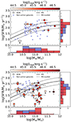 |
Fig. B.1. Comparison of SFR and stellar mass of AGN host galaxies (red circles) and non-active galaxies of the control sample (blue squares) for low-z bin (z = 1 − 1.8; Top) and high-z bin (z = 1.8 − 2.55; Bottom). Red circles are color-coded based on their AGN bolometric luminosity, as retrieved from SED fitting from this work or from the literature. The solid line marks the MS at the mean redshift of each bin from Schreiber et al. (2015) and dashed lines show its scatter (equal to 0.3 dex). The distribution of SFR (right) and M* (bottom) for AGN (red) and non-active galaxies (blue) in the side panels are intended for illustration purposes only, since the upper limits are considered at face value. A robust comparison of the distribution of SFR and M* applying the hierarchical method described in Sect. 5.2 is presented in Fig. B.2. |
We compare the total posterior distributions of M* and SFR of AGN hosts and non-active galaxies of the full samples and devided in the two redshift bins used to match the two samples. The M* and SFR distributions of AGN hosts and non-active galaxies were built applying the Bayesian hierarchical method used for the molecular gas fractions, as described in Sect. 5.2. The KS test returns a p-value larger than 5% for all cases but the high-z bin of SFR. Figure B.2 shows the total posterior distributions of both samples and all the considered redshift ranges.
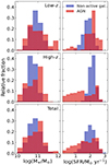 |
Fig. B.2. Total posterior distributions of M* (left) and SFR (right) of AGN hosts (AGN sample 1, red) and non-active galaxies (blue). The comparison is carried out for low-z bin, high-z bin and full redshift range, from top to bottom. |
Appendix C: ALMA data analysis of KASHz AGN
We present in this section the ALMA data analysis and some notes about single sources. Table E.1 summarizes the info of all KASHz ALMA targets. The KASHz molecular sample includes also:
-
Four5 AGN that are shared with SUPER that were not presented in C21 because data became available later on;
-
The ALMA observations of cdfs_278, cdfs_419 and cdfs_614 that were recently presented in Yang et al. (2022);
-
The ALMA program 2018.1.00251.S (PI: M. Brusa) covering CO(2–1) (and CO(5-4)) of lid_1639 (XID5395, Brusa et al. 2016), the analysis of which will be presented in Ricci et al. (2024, in prep.);
-
A few AGN that are already well known for their gas kinematics and AGN feedback properties: lid_1565 (XID2028, Cresci et al. 2015; Brusa et al. 2018; Scholtz et al. 2020; Cresci et al. 2023; Veilleux et al. 2023), cdfs_587 (GMASS0953, Popping et al. 2017; Talia et al. 2018; Loiacono et al. 2019), cdfs_794 (ALESS067.1, Chen et al. 2017; Calistro Rivera et al. 2018).
Our ALMA cube analysis was performed as follows: i) we identify the source emission by finding the peak emission in the vicinity of the coordinates of the target in the line velocity-integrated map produced with the channels at ±1000 km/s around the expected line frequency peak based on the source redshift, with a visual assessment that the identified peak is not associated with random noise; ii) we extract the source spectrum from the peak spaxel or, in case of partially resolved emission, from the aperture that maximizes the signal-to-noise ratio on the moment 0 map and than divided by the beam size in pixels; iii) we fit the line with one Gaussian to measure its centroid and FWHM; iv) we re-center the cube to the observed frequency and produce the line velocity-integrated (0th order) moment maps on a spectral range corresponding to ±3× the line width σ; v) we extract the spectrum from the re-centered cube, re-selecting the spectrum extraction area (or peak pixel) on the new 0th-moment map, and we rebin it to a channel width that samples the FWHM of the line at least 7 times, chosen as best trade-off to also maintain a good signal-to-noise ratio; vi) lastly, we fit the line with a single- and a double-Gaussian function, storing the respective parameters and relative errors. Regarding step v), the spectrum is extracted from the 3σ mask of the target in the moment 0 map in case this is larger than the corresponding beam, otherwise the spectrum is extracted from the peak pixel of the line velocity-integrated map produced in step iv). We derive the uncertainty of the integrated CO flux from the root-mean square noise (rms) of the line-free range of the spectrum (rmsspec):  , where Δv is the channel width in km s−1. We produced the final cubes by setting a channel width that allows us to sample the line FWHM at least 7 times in the tclean, chosen as the best trade-off to sample the line profile while maintaining a good signal-to-noise ratio. We consider a source as detected if its emission peak in the velocity-integrated map is at least 3 times the rms of the map.
Summary of the ALMA observations reduced and analyzed in this work.
Almost all of our CO lines are well fitted by a single Gaussian component based on the F-test, a commonly used statistical test to compare the goodness of two fits through their χ2 and degrees of freedom. For the purposes of our study and having checked that the single- and double-Gaussian models return consistent values, we refer to the results obtained with the single-Gaussian modeling as a measure of the total CO flux of our host galaxies. We report the velocity integrated map (derived in the ±3×FWHM, with FWHM = 300 km s−1) and spectrum of cid_108 in Fig. 3 as example of CO detections. Maps and spectra of the rest of the sample are available on Zenodo6.
As a sanity check of the robustness of our ALMA analysis, we compared the CO flux derived from the spectral fits with the flux obtained integrating over the spectrum extraction region in the moment 0 maps (either the peak pixel value or the flux in the 3σ mask in case this is smaller or larger than the corresponding beam, respectively) and as derived from the 2D fits of the moment 0 maps with the CASA task imfit. The CO flux measured from the spectral fits is well consistent with both estimates from the moment 0 maps for all targets, with the exception of the CO emission of cdfs_794. The value measured with imfit is consistent with that obtained by Calistro Rivera et al. (2018), where the spectrum was extracted using a circular region of 1″ radius, which is underestimated by the flux obtained from the spectrum extracted from the 3σ mask. We thus re-extracted the spectrum using the same approach as in Calistro Rivera et al. (2018) and find a CO(3–2) flux that is consistent with the value integrated from the 1″ circle, the 2D fit result of imfit and that of Calistro Rivera et al.. The CO properties of cdfs_794 presented in this paper are thus those corresponding to the 1″-circle spectrum extraction region.
We define non-detections the sources with S/N≲3 in the velocity-integrated maps (11 CO lines of 10 KASHz AGN). For the non-detections, we assume a FWHM = 300 km s−1 (e.g., D’Amato et al. 2020; Pensabene et al. 2021), consistent with the median FWHM of the detected targets, and estimate the flux upper limits as  , where rmsp is the rms of the peak channel in the cube with channel width of Δv = 40 km s−1 and n is the number of channels sampling the FWHM (i.e., n = 7.5 for Δv = 40 km s−1 and FWHM of 300 km s−1). Velocity integrated maps derived in the ±3 FWHM (with FWHM = 300 km s−1) and spectra of non-detections are available on Zenodo7.
We assessed the continuum emission of our targets with the tclean task of CASA 6.4 used in “mfs” mode on line-free channels of all the available spectral windows. Two AGN are detected in continuum (see Table E.3). We measure the continuum flux from the peak pixel in the continuum map or from the 3σ mask if this is more extended than one beam. Regarding continuum non-detections, we report in Table E.3 the 3σ upper limit. The photometric points obtained from ALMA Band 3 and 4 continuum are included in the SED fitting of the KASHz molecular sample (see Appendix D).
Appendix D: SED fitting of KASHz and SUPER AGN
We measure the stellar mass M*, the FIR luminosity LFIR of the host galaxies and the AGN bolometric luminosity Lbol of the KASHz ALMA targets by performing SED fitting with CIGALE v.2022.1 (Boquien et al. 2019; Yang et al. 2020), a publicly available, python-based SED-fitting code. We also update the SED fitting of the SUPER AGN presented in C21 that are drawn from the CDFS and COSMOS fields, to take advantage of the new photometry releases from the parent-survey collaborations (see Sect. D.2).
D.1. CIGALE SED fitting code
The CIGALE code adopts a multicomponent fitting approach to separate the AGN contribution from the galaxy emission. It employs model templates that encompass nebular emission, dust-attenuated stellar emission, dust emission driven by star formation, and AGN emission spanning from X-rays to radio wavelengths, including both the primary accretion disk emission and the emission reprocessed by the dusty torus surrounding the central engine. This is an “energy-balance” code, meaning that it takes into account the energy balance between the UV-optical attenuation and the FIR re-emission by dust. The code provides the values of the parameters of interest (as selected by the user) in two ways. The first corresponds to the solution returning the lowest χ2, and the second to the output of a Bayesian-like analysis, for which the returned value of each parameter corresponds to the mean value of the probability distribution function (PDF) built accounting for all the different models that are used in the fitting process. In this work, we refer to the Bayesian output as the best-fit SED. One of the major updates in the code was the inclusion of the X-ray module 8, which allows us to set a prior on the αOX9 of the AGN by feeding the code with the intrinsic (i.e., absorption corrected) X-ray fluxes. Since the AGN X-ray emission significantly surpasses that of the host galaxy, such a prior assumption allows us to delimit the range of AGN UV luminosity for a chosen scatter with respect to the αOX-L2500 Å relation (e.g., Lusso & Risaliti 2016; Martocchia et al. 2017), and thus to better decouple the emission of galaxy and AGN in this range. We use the same setup of models presented in C18 to reduce the possible sources of systematics between the KASHz and SUPER AGN: stellar population models with solar metallicity (Bruzual & Charlot 2003), a delayed SF history, the modified Calzetti et al. (2000) attenuation law and a Chabrier (2003) initial mass function, plus the nebular emission following Inoue (2011), Nagao et al. (2011). We model the contributions from the cold dust associated with star formation and AGN emission with the libraries of Dale et al. (2014) and Fritz et al. (2006), with updates from Feltre et al. (2012), respectively. Thus, the main difference between our SED-fitting setup and that of C21 resides in the inclusion of the X-ray module.
D.2. Updates on multiband photometry
We collect the Near-UV to FIR photometry referring to the latest Near-UV-to-FIR multiwavelength catalogs provided by the collaborations of the deep surveys our targets are extracted from:
-
COSMOS: We retrieve the Near-UV/optical to MIR photometry from COSMOS2020 (catalog version: classic Weaver et al. 2022); we complement the multiwavelength info of our COSMOS targets with the “super-deblended” FIR to (sub-)mm photometric catalog of Jin et al. (2018). Two sources of the KASHz molecular sample (lid_1565, cid_72) are not included in the superdeblended catalog, thus, following C18, we collect their 24–500 μm photometry from the previous PACS Evolutionary Probe (PEP) and Herschel Multi-tiered Extragalactic Survey (HerMES) DR4 catalogs by Lutz et al. (2011) and Hurley et al. (2017), respectively, using a match radius of 2″. Moreover, cid_72 has only one match in the COSMOS2020 catalog at a distance of 6″ from the coordinates listed in Marchesi et al. (2016), while the best match with the COSMOS2015 source list (Laigle et al. 2016) falls at less than 0.5″. We thus collect the Near-UV/optical to MIR photometry of cid_72 from COSMOS2015;
-
CDFS: we collect the Near-UV to MIR photometry from the ASTRODEEP-GS43 catalog of the CANDELS/GOODS-S field (Cosmic Assembly Near-infrared Deep Extragalactic Legacy Survey/Great Observatories Origins Deep Survey-South, Merlin et al. 2021). FIR photometry is retrieved from the Herschel Extragalactic Legacy Project (HELP) collaboration (Shirley et al. 2019, 2021). , As done for COSMOS targets, we complement the FIR photometry of CDFS AGN that are not included in the HELP catalog (cdfs_313, cdfs_522) with previous results from PEP and HerMES 10 (Oliver et al. 2012; Hurley et al. 2017);
-
X-UDS: we collect the Near-UV to FIR photometry from the “best photometry” catalog compiled by the HELP collaboration (N-UV to MIR source catalogs used by the HELP collaboration: Almaini et al. 2007; Furusawa et al. 2008; Tudorica et al. 2017).
We include in the photometry of our sources also the ALMA continuum photometric points (or upper limits), from Band 3 to Band 7, when available, either drawn from this work (see Table E.3) or from Scholtz et al. (2018), Lamperti et al. (2021) and C21. Given the significant update in terms of SED sampling, flux depth and photometry extraction of the available photometry for COSMOS and CDFS targets, we also refit the SED of the SUPER targets in C21 drawn from these two surveys (see Table E.2) for consistency. We flag as upper limits all the HELP FIR fluxes below the 2σ level and feed to CIGALE the corresponding 3σ level value as upper limit. We consider those above the 2σ limit as reliable based on the implementation of the flux extraction procedure by HELP collaboration, which uses the optical/NIR position of a target as prior to deblend its flux in the FIR bands. The “Super-deblended” catalog already flags the upper limits, thus we follow their classification, with the only exception of cid_1205: the source is placed in a crowded field, thus its FIR photometry is well detected but highly contaminated by a nearby source. We flag all the Superdeblended filters of cid_1205 as upper limits. For the X-ray prior to work, one has to feed CIGALE with the absorption-corrected (i.e., intrinsic) X-ray fluxes. We compute the X-ray photometric points in the 0.5–2 keV and 2–10 keV observed energy range from the rest-frame, absorption-corrected X-ray luminosity using the intrinsic photon index, either obtained from the direct fit of the X-ray spectra from the literature (for CDFS and COSMOS targets, Lanzuisi et al. 2013, 2015; Liu et al. 2017, C18,C21) or as derived by the X-ray deep survey collaborations in the survey catalogs (Luo et al. 2017; Akiyama et al. 2015; Kocevski et al. 2018; Marchesi et al. 2016), as flagged in Table E.1. Since the survey catalogs do not provide an uncertainty for the intrinsic X-ray luminosity, we assigned a uniform ±30% uncertainty for each X-ray photometric point in our sample. The mean (and median) uncertainty of the observed fluxes in the COSMOS-Legacy field is ≃20% (Civano et al. 2016), thus here we include a mean 10% to account for additional uncertainties due to the absorption correction. The photometric bands used for each of the X-ray deep fields are listed in Table E.4. We summarize in Table E.5 all the model parameters that were set to a value different than the default of X-CIGALE in our SED fitting runs. We note that the chosen X-CIGALE setup tests ∼290M SED models for each source.
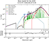 |
Fig. D.1. Observed-frame, best-fit SED models of lid_1639. Purple empty circles mark observed flux densities, purple empty triangles the observational upper limits and red filled circles indicate the best-fit model prediction. Yellow (blue dashed) lines are for the stellar (un)attenuated emisson; green lines for the nebular emission; red lines for dust emission; orange lines for the AGN component and black lines for the total, best-fit model. The SEDs of the rest of the AGN sample are available on Zenodo at the following link: https://doi.org/10.5281/zenodo.13149280. |
D.3. Highlights and caveats on the results
The results obtained with the described photometry and CIGALE setup provide adequate fits of the SEDs of our targets, based on the reduced χ2 value and the overall agreement between the best-fit model and the photometry throughout the full X-ray-to-FIR band (see Table E.2 and Fig. D.1 12), with the exception of cdfs_313. Moreover, Mountrichas et al. (2021) and Buat et al. (2021) show that if there is a large discrepancy between the mean of the posterior distribution and the best-fit value of a certain parameter of CIGALE, then the result for that parameter is not reliable. We checked for such a consistency in M*, SFR and LAGN (i.e., Lbol). All of our results match the acceptance range defined by the authors (that is, the ratio of the Bayesian and the best-fit value falls in the 0.5–5 range). We managed to obtain a good fit of the SED of cdfs_313 by removing the X-ray part of the SED: it is possible that the X-ray flux, and thus the link set by CIGALE with the UV emission of this target, was not representative of the AGN accretion, for instance due to the low number of counts in the CDFS spectrum (25 ± 5 cts, Luo et al. 2017) or to faster source variability in the X-rays compared to the rest of the SED.
We compared the results for SUPER AGN to those of C18 and C21. For most of the targets, the main parameters of interest for our analysis, which are M*, LFIR and LAGN, are consistent with those of C18 and C21 within the typical uncertainties derived by Pacifici et al. (2023) (0.1dex in stellar mass and 0.3dex in SFR, hence LFIR for our purposes). A few targets present a larger difference with respect to the SED fitting of C18 and C21, but this can be explained as being due to the updated SED fitting code (e.g., the inclusion of the X-ray module) and the update in the photometry, especially in the FIR band.
We checked the agreement between the best-fit SED of lid_1639 and the ALMA photometry in Band 6 (Ricci et al., 2024 in prep). The redward side of the FIR bump is well consistent with the flux in ALMA Band 6, however, given the good sampling of the FIR band for this source, we decided to exclude ALMA Band 6 from its filter set because of the high resolution of the observation (∼0.6″), which might underestimate the target flux by missing the emission at larger scales. A different case is instead cid_1205: since we have considered all of its FIR data as upper limits, we decided to include the ALMA Band 7 flux of Lamperti et al. (2021) despite the even higher resolution of the corresponding observation (∼0.2″). We consider this as the best choice to not overestimate the FIR bump of this system, also supported by the fact that Lamperti et al. conclude that their ALMA Band 6 fluxes mostly sample emission due to dust heated by SF.
Lastly, for some of the very near-UV-bright broad-line AGN in our sample, we can only constrain an upper limit to the stellar mass. Since the optical/NIR galaxy emission is outshined by the AGN, there is a strong degeneracy between the AGN component and the stellar component which can unfortunately result in stellar masses constrained only as upper limits, which we estimate at 3σ.
Appendix E: Tables
Summary of KASHz ALMA targets
Summary of the properties of the AGN sample.
Summary of results from the ALMA data analysis of KASHz AGN analyzed in this work
Summary of the photometric data used for the SED-fitting modeling described in Appendix D.
Input parameter values used for the SED-fitting procedure in Appendix D.
All Tables
Summary of results from the ALMA data analysis of KASHz AGN analyzed in this work
Summary of the photometric data used for the SED-fitting modeling described in Appendix D.
All Figures
|
Fig. 1. Luminosity versus redshift distribution of the AGN samples used in this work. Top: intrinsic 2–10 keV rest-frame X-ray luminosity LX vs. redshift z distribution of the full KASHz (purple pentagons) and SUPER (blue circles) surveys. SUPER ALMA targets are from C21. The side panel shows the density distribution of SUPER (blue) and KASHz (purple) targets. Bottom: bolometric luminosity LBol vs. redshift z distribution of the AGN targeted by ALMA and included in this work. For the KASHz (purple pentagons) and SUPER (blue circles) targets included in this panel, the bolometric luminosity was derived from SED fitting in this work (see Appendix D), in C18, and in C21. The side panel shows the density distribution of the samples. The black dots mark the six targets discarded because they were missing at least one parameter of interest for our analysis; the white dots mark the three targets that do not allow fgas to be computed. |
| In the text | |
|
Fig. 2. Comparison of star formation rate and stellar mass of the AGN host galaxies (red circles) and the non-active galaxies of the control sample (blue squares). The red circles are color-coded based on their AGN bolometric luminosity, as retrieved from SED fitting from this work or from the literature. The solid line is the MS at z = 2 from Schreiber et al. (2015) and dashed lines show its scatter (equal to 0.3 dex). The distribution of SFR (right) and M* (bottom) for AGN (red) and non-active galaxies (blue) in the two side panels are intended for illustration purposes only since the upper limits are considered at face value. A robust comparison of the distribution of SFR and M* applying the hierarchical method described in Sect. 5.2 is presented in Fig. B.2. |
| In the text | |
|
Fig. 3. CO line velocity-integrated emission map (left) and spectrum (right) of cid_108. The solid contour levels in the left panels start at 2σ and increase linearly. The dashed contours indicate the [−3,−2]×σ level. The beam of each observation is shown by the gray ellipse in the bottom left corner of each map. CO maps and spectra of the rest of the AGN sample are available on Zenodo at the following link: https://doi.org/10.5281/zenodo.13149280 |
| In the text | |
|
Fig. 4. CO luminosity vs. FIR luminosity bisector fits of AGN host galaxies (red circles) and non-active galaxies of their control sample (blue squares). The thick lines mark the bisector fits obtained by adopting a Bayesian framework (see main text). The dispersion of the fits is given by plotting 500 realizations of the bisector fits. The vertical axis on the right is derived by assuming αCO = 3.6 M⊙/(K km s−1 pc2) and serves for illustration purposes only, since we only consider L′CO in our quantitative analysis (see Sect. 5.1). |
| In the text | |
|
Fig. 5. Corner plots of best-fit parameters for the log( |
| In the text | |
|
Fig. 6. Distribution of L′CO/M* (observational proxy of the gas fraction fgas) for AGN host galaxies (red) and non-active galaxies of the control sample (blue). Upper panel: filled histograms show the total distributions, obtained by joining the sampled posterior distribution of each target for both samples. The blue squares indicate the measure of each non-active galaxy (98 targets), red circles that of each AGN (40 targets). The blue and red triangles indicate upper limits if pointing leftward and lower limits if pointing rightward for the gas fraction of non-active galaxies and AGN, respectively. Lower panel: violin plots show the sampled posterior distribution of the mean of the hierarchical Gaussian prior used in our Bayesian analysis. The diamonds show the measured mean value μfgas of AGN (red) and non-active galaxies (blue). The top axis is derived by assuming αCO = 3.6 M⊙/(K km s−1 pc2) and serves for illustration purposes only since we only consider L′CO in our quantitative analysis (see Sect. 5.2). |
| In the text | |
|
Fig. 7. CO luminosity vs. stellar mass bisector fits of AGN host galaxies (red circles) and non-active galaxies of the control sample (blue squares). The thick lines mark the bisector fits obtained by adopting a Bayesian framework (see main text). The dispersion of the fits is given by plotting 500 realizations of the bisector fits. The vertical axis on the right is derived by assuming αCO = 3.6 M⊙/(K km s−1 pc2) and serves for illustration purposes only since we only consider L′CO in our quantitative analysis (see Sect. 5.3). |
| In the text | |
|
Fig. 8. Gas fraction vs. stellar mass bisector fits of AGN host galaxies (red circles) and non-active galaxies of the control sample (blue squares). The thick lines mark the bisector fits obtained by adopting a Bayesian framework (see main text). The dispersion of the fits is given by plotting 500 realizations of the bisector fits. The vertical axis on the right is derived by assuming |
| In the text | |
|
Fig. 9. Distribution of gas fraction fH2 vs. bolometric luminosity Lbol. Galaxies in the simulations are selected to match the observed parameter range in stellar mass and SFR, and to host AGN with Lbol > 1044.3 erg s−1 and λEdd > 0.01. Contours contain 90% of the selected systems and extreme outliers are shown as individual points. The color-coding for the simulations is as follows: EAGLE, TNG, and SIMBA in purple, red, and orange, respectively. Observational points are shown as gray pentagons for KASHz AGN (presented in this work) and gray circles for SUPER AGN from C21, scaled by αCO = 3.6 M⊙ (K km s−1 pc2)−1. The black arrow marks the downward shift for αCO = 0.8 M⊙ (K km s−1 pc2)−1. The bottom left point shows the mean error bar of the observational sample. |
| In the text | |
|
Fig. 10. Comparison of molecular gas fraction against SFR of AGN (red) and non-active galaxies (blue) from observations and simulations. SUPER ALMA targets are shown as red circles, KASHz AGN as red pentagons, and observed non-active galaxies as blue squares. Blue downward triangles and red upward triangles show the median and 16th–84th percentiles of non-active galaxies and AGN in the simulations, respectively, grouped in SFR bins of 0.3 dex. Hexagons show the distribution of simulated AGN and are color-coded based on the mean stellar mass of the host galaxies in each bin. Observed molecular gas fractions are computed assuming αCO = 3.6 M⊙ (K km s−1 pc2)−1. Galaxies in the simulations are filtered to match the observed properties of the observed galaxies. The black arrow marks the downward shift for αCO = 0.8 M⊙ (K km s−1 pc2)−1. |
| In the text | |
|
Fig. 11. Gas fraction distributions of AGN host galaxies (filled violin plots) and non-active galaxies (hatched violin plots) from cosmological simulations (EAGLE, TNG, and SIMBA in purple, red, and orange, respectively) and observations presented in this work (gray), scaled for αCO = 3.6 M⊙ (K km s−1 pc2)−1. The diamond markers give the mean value of each distribution. Gas fraction distributions from the observations correspond to the total gas fraction distributions built in Sect. 5.2. Galaxies in the simulations are filtered as in Fig. 9. The black arrow marks the leftward shift of observed distributions (black) for αCO = 0.8 M⊙ (K km s−1 pc2)−1. |
| In the text | |
|
Fig. B.1. Comparison of SFR and stellar mass of AGN host galaxies (red circles) and non-active galaxies of the control sample (blue squares) for low-z bin (z = 1 − 1.8; Top) and high-z bin (z = 1.8 − 2.55; Bottom). Red circles are color-coded based on their AGN bolometric luminosity, as retrieved from SED fitting from this work or from the literature. The solid line marks the MS at the mean redshift of each bin from Schreiber et al. (2015) and dashed lines show its scatter (equal to 0.3 dex). The distribution of SFR (right) and M* (bottom) for AGN (red) and non-active galaxies (blue) in the side panels are intended for illustration purposes only, since the upper limits are considered at face value. A robust comparison of the distribution of SFR and M* applying the hierarchical method described in Sect. 5.2 is presented in Fig. B.2. |
| In the text | |
|
Fig. B.2. Total posterior distributions of M* (left) and SFR (right) of AGN hosts (AGN sample 1, red) and non-active galaxies (blue). The comparison is carried out for low-z bin, high-z bin and full redshift range, from top to bottom. |
| In the text | |
|
Fig. D.1. Observed-frame, best-fit SED models of lid_1639. Purple empty circles mark observed flux densities, purple empty triangles the observational upper limits and red filled circles indicate the best-fit model prediction. Yellow (blue dashed) lines are for the stellar (un)attenuated emisson; green lines for the nebular emission; red lines for dust emission; orange lines for the AGN component and black lines for the total, best-fit model. The SEDs of the rest of the AGN sample are available on Zenodo at the following link: https://doi.org/10.5281/zenodo.13149280. |
| In the text | |
Current usage metrics show cumulative count of Article Views (full-text article views including HTML views, PDF and ePub downloads, according to the available data) and Abstracts Views on Vision4Press platform.
Data correspond to usage on the plateform after 2015. The current usage metrics is available 48-96 hours after online publication and is updated daily on week days.
Initial download of the metrics may take a while.