| Issue |
A&A
Volume 690, October 2024
|
|
|---|---|---|
| Article Number | A15 | |
| Number of page(s) | 11 | |
| Section | Galactic structure, stellar clusters and populations | |
| DOI | https://doi.org/10.1051/0004-6361/202451387 | |
| Published online | 26 September 2024 | |
Limitations and rotation of the two-armed phase spiral in the Milky Way stellar disc
1
Lund Observatory, Division of Astrophysics, Department of Physics, Lund University,
Box 118,
221 00
Lund,
Sweden
2
School of Physics & Astronomy, University of Leicester,
University Road,
Leicester
LE1 7RH,
UK
Received:
5
July
2024
Accepted:
17
August
2024
Abstract
Context. The Milky Way’s history of recent disturbances is vividly demonstrated by a structure in the vertical phase-space distribution known as the Gaia phase spiral. A one-armed phase spiral has been seen widely across the Milky Way disc, while a two-armed one has only been observed in the solar neighbourhood.
Aims. This study aims to determine the properties of the two-armed phase spiral and to put it in a Galactic context, with the ultimate goal of understanding the structure and history of the Milky Way disc.
Methods. The Gaia DR3 data were used to trace and characterise the two-armed phase spiral. Special focus was put on the phase spiral’s spatial distribution, rotational behaviour, and chemical characteristics. To quantify the properties of the phase spiral, we used a model that fits a spiral pattern to the phase space distribution of the stars.
Results. We found that the two-armed phase spiral is detectable only within a narrow range of galactocentric distances and angular momenta in the solar neighbourhood, R = 8 ± 0.5 kpc, LZ = 1450 ± 50 kpc km s−1. Outside this region, the phase spiral is one-armed. The two-armed phase spiral rotates with the phase angle, in a similar way to the one-armed phase spiral, and changes axis ratio with phase angle. Additionally, stars within the phase-space overdensity caused by the two-armed phase spiral pattern have slightly higher mean metallicity than stars in the underdense regions of the pattern at equivalent galactocentric distances, angular momenta, and vertical orbit extents.
Conclusions. The two-armed phase spiral rotates with phase angle and its effect can be seen in metallicity, in a similar way to the one-armed phase spiral. However, the limited range over which it can be found, and its variation in shape are quite different from the one-armed version, suggesting it is a much more localised phenomenon in the Galactic disc.
Key words: Galaxy: disk / Galaxy: evolution / Galaxy: kinematics and dynamics / solar neighborhood / Galaxy: structure
Corresponding author; This email address is being protected from spambots. You need JavaScript enabled to view it.
© The Authors 2024
 Open Access article, published by EDP Sciences, under the terms of the Creative Commons Attribution License (https://creativecommons.org/licenses/by/4.0), which permits unrestricted use, distribution, and reproduction in any medium, provided the original work is properly cited.
This article is published in open access under the Subscribe to Open model. This email address is being protected from spambots. You need JavaScript enabled to view it. to support open access publication.
1 Introduction
The processes that reshape galaxies such as the Milky Way, such as mergers (e.g. White & Rees 1978) and the creation and influence of bars and spiral arms (e.g. Lindblad 1941; Sellwood & Binney 2002) cause disequilibrium within galaxies. Studying this disequilibrium in the Milky Way gives us the best chance of understanding how these processes operate.
The quantity and quality of astrometric and spectroscopic data from the European Space Agency’s Gaia mission (Gaia Collaboration 2016a,b, 2018, 2021a, 2023), has revolutionised our access to the Milky Way’s structure in recent years and has allowed astronomers to study our Galaxy in greater detail than ever before. Antoja et al. (2018) discovered the “phase spiral” or “snail shell” in the velocity-space distribution of stars in the second Gaia data release. The phase spiral is an unevenness in the distribution of vertical velocities of stars in the Galactic disc, which takes the form of a spiral when viewed in a vertical phase space diagram with Z and VZ on the axes. Subsequent investigations have expanded upon these findings, exploring the phase spiral’s extent, morphology, and dependence on age or metallicity. These have shown that the phase spiral covers a smaller range in vertical velocity with increasing galactocentric radius (e.g. Laporte et al. 2019; Antoja et al. 2023), rotates with position around the galaxy (e.g. Alinder et al. 2023), and has higher contrast in the inner regions for younger, more metal-rich stars (Bland-Hawthorn et al. 2019).
The origin of the phase spiral is a subject of active discussion. Suggested theories include the impact of the Sagittarius dwarf galaxy’s passage through the Milky Way disc (Binney & Schönrich 2018; Laporte et al. 2019; Bland-Hawthorn et al. 2019), and waves induced by a change in the pattern speed of the bar (Li et al. 2023). The possibility that there are multiple causes behind the observed phenomenon has emerged in recent years. Hunt et al. (2022); Bennett et al. (2022) and Tremaine et al. (2023) all suggest that the formation history of the phase spiral cannot be explained with a single impact but perhaps from several smaller disturbances. Frankel et al. (2023) and Antoja et al. (2023) both find that a simple model with a single cause for the perturbation fails to explain the observations and calls for more complex models.
The first mention of two-armed phase spirals in the literature is in the N-body merger simulations of Hunt et al. (2021) where they show up as the result of an interaction with an external perturber. These two-armed spirals are relatively short-lived, but the authors claim that traces of them might still be found in the outer Galactic disc which preserves dynamical structures for longer. In Hunt et al. (2022), however, the two-armed phase spiral was seen in Gaia data release 3 (DR3) in solar neighbourhood stars (with heliocentric distances less than 1 kpc) with a guiding centre radius (RG) of about 6.33 kpc. The concept of the guiding centre comes from epicycle theory, in which the orbital motion of a star can be decomposed into a guiding centre on a large circular orbit with the same angular momentum as the star, and a small epicyclic elliptical excursion around this centre. Even for substantially non-circular orbits, we can still use this concept as a convenient description via action-angle coordinates (e.g. Binney & Tremaine 2008), with the position of the guiding centre being associated with the azimuthal action (that is, the angular momentum) and its conjugate angle. Hunt et al. (2022) investigated the phase spiral as a function of RG and azimuthal angle of the guiding centre (θϕ) and detected phase spirals with both one and two arms.
Using an N-body simulation of an isolated Milky Way-like galaxy, Hunt et al. (2022) found that this sort of system forms a two-armed phase spiral in the inner regions of the galaxy, but no one-armed phase spiral. Grand et al. (2023) conduct a cosmological simulation of a Milky Way-like galaxy experiencing an interaction with an external, Sagittarius-like, perturber. This simulation shows transient two-armed phase spirals appearing in different regions of the galaxy. Li et al. (2023) investigate how an isolated spiral galaxy can form phase spirals. Central to their analysis is the concept of “pattern speed”, defined here as the rate at which the structure of the bar rotates. They find that an isolated spiral galaxy containing a bar with constant pattern speed does not form any phase spirals, despite producing a vertical perturbation in the galaxy’s disc, called a “breathing mode”, which is usually associated with two-armed phase spirals (Widrow 2023). When they introduce a bar with a decreasing pattern speed, a two-armed phase spiral is created. They claim that a galaxy with internal non-axisymmetric structures with a constant pattern speed will not produce the observed structures in vertical motion when encountering an external perturber.
This paper aims to address some key questions about the characteristics of the two-armed phase spiral in the Milky Way. Specifically, we seek to determine where in the Galaxy and where in phase space this two-armed phase spiral can be found, how it varies with different parameters such as azimuthal angle (ϕ), phase angle (θϕ), and angular momentum (LZ). We will further investigate whether it has any characteristic appearance in metallicity space. It is our belief that, by establishing the behaviour of the two-armed phase spiral and comparing it to that of the one-armed phase spiral, we can gain insights into the dynamical processes shaping our Galaxy and the interplay between these processes and the Galactic chemical environment.
We begin by describing the selection and analysis of the stellar sample in Sec. 2. In Sec. 3 we present the methods we utilise in searching for and characterising the two-armed phase spiral, and the results. Our interpretation and discussion of the results are presented in Sec. 4, where we put our findings into a broader context. Finally, Sec. 5 summarises our key conclusions and the implications they may have for our understanding of the assembly and evolution of our Galaxy.
2 Data
2.1 Astrometic data
We used a standard coordinate system1 and Gaia DR3 to get the position and velocities (Gaia Collaboration 2016b, 2023) of stars, with distances calculated by Bailer-Jones et al. (2021), who used a Bayesian approach with a direction-dependant prior on distance, the measured parallaxes, Gaia photometry, and the fact that stars of different colours have different ranges of probable absolute magnitudes to re-compute the distances.
When querying the public Gaia database2, we required parallax_over_error>=3 as this removes the most uncertain distance estimates. The query used resulted in 31552449 stars being selected. The full ADQL-query used to retrieve these data was:
SELECT source_id, ra, dec, pmra, pmdec,
r_med_photogeo, radial_velocity,
pmra_error, pmdec_error, parallax_error, teff_gspphot
FROM external.gaiaedr3_distance
JOIN gaiadr3.gaia_source USING (source_id)
WHERE parallax_over_error>=3
and radial_velocity IS NOT NULL
and r_med_photogeo IS NOT NULL
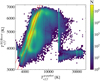 |
Fig. 1 Comparison of |
![Mathematical equation: $\[T_{\mathrm{eff}}^{{gspphot }}\]$](/articles/aa/full_html/2024/10/aa51387-24/aa51387-24-eq1.png)
![Mathematical equation: $\[T_{\mathrm{eff}}^{{xgboost }}\]$](/articles/aa/full_html/2024/10/aa51387-24/aa51387-24-eq2.png)
![Mathematical equation: $\[\left|T_{\mathrm{eff}}^{{gspphot }}-T_{\mathrm{eff}}^{{xgboost }}\right|<500 \mathrm{~K}\]$](/articles/aa/full_html/2024/10/aa51387-24/aa51387-24-eq3.png)
2.2 Metallicity data
Andrae et al. (2023) used a machine learning algorithm called XGBoost to derive stellar metallicities, Teff, and log(g) for more than 120 million stars in the Gaia catalogue based on data from its low-resolution XP spectra. From these data, we selected the 25 050 958 stars that are also present in our selection from the Gaia database.
To address inaccuracies in classifying stars with high effective temperatures (Teff > 7000 K), due to the lack of such stars in the Andrae et al. (2023) training data, we applied additional cuts to the data. We compared the effective temperature within Gaia DR3 (GSP-Phot) to that reported by XGBoost. The discrepancy between the effective temperatures reported by Gaia’s GSP-Phot and those predicted by the XGBoost algorithm is highlighted in Fig. 1. Significant mismatches are observed for stars with ![Mathematical equation: $\[T_{\text {eff }}^{{gspphot }}>10~000 \mathrm{~K}\]$](/articles/aa/full_html/2024/10/aa51387-24/aa51387-24-eq4.png) in particular.
in particular.
To leave a clean sample we removed all stars that are listed as variables in the Gaia catalogue because their temperature estimates are uncertain as Teff varies with pulsation phase. Then, all stars with a difference in effective temperature ![Mathematical equation: $\[\mid T_{\mathrm{eff}}^{{gspphot }}-T_{\mathrm{eff}}^{{xgboost }} \mid>500 \mathrm{~K}\]$](/articles/aa/full_html/2024/10/aa51387-24/aa51387-24-eq5.png) were removed. Doing this cut also effectively removed all stars with
were removed. Doing this cut also effectively removed all stars with ![Mathematical equation: $\[T_{\mathrm{eff}}^{{gspphot }} \gtrsim 7000 \mathrm{~K}\]$](/articles/aa/full_html/2024/10/aa51387-24/aa51387-24-eq6.png) from our sample. This left a sample of 15 575635 stars with metallicity data. The dashed red lines in Fig. 1 show this region.
from our sample. This left a sample of 15 575635 stars with metallicity data. The dashed red lines in Fig. 1 show this region.
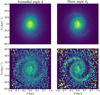 |
Fig. 2 Comparison of phase spiral clarity when selecting stars based on azimuthal angle (ϕ, left column) and azimuthal angle of the guiding centre or phase angle (θϕ, right column), and using a Gaussian filter (bottom row) compared to not using one (top row). We can note that the right column, particularly the bottom row, has a much clearer spiral pattern than the rest. The plots show number density and number density contrast in the Z − VZ phase plane of stars in the solar neighbourhood (d < 1 kpc) with a further selection by ϕ or θϕ. The left column shows stars with 175° < ϕ < 185° and the right column shows stars with 175° < θϕ < 185°. All stars have 1400 < LZ/kpc km s−1 < 1500. |
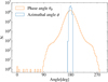 |
Fig. 3 Comparison of the distributions of azimuthal angle ϕ and azimuthal angle of guiding centre θϕ for stars in the solar neighbourhood (d < 1 kpc). |
3 Characterising the two-armed phase spiral
3.1 Data processing
Following Hunt et al. (2021), who showed that dividing a sample of stars by the azimuthal angle of their guiding centres (also called the phase angle, θϕ) reveals phase spiral patterns more clearly than dividing by the azimuthal angles of the stars themselves (ϕ), we computed action-angle variables for our sample. We used the galactic dynamics package AGAMA (Action-based Galaxy Modelling Architecture, Vasiliev 2019) with the best potential from McMillan (2017).
A Gaussian filtering technique was used to enhance the contrast of the phase spiral in our plots. We utilised the scipy.ndimage.gaussian_filter function from the SciPy library (Virtanen et al. 2020) to create a blurred version with the Gaussian filter and dividing the original with it. In this way, the spiral pattern was enhanced.
Figure 2 compares four plots of the phase spirals in the solar neighbourhood to demonstrate the effect that a Gaussian filter and the choice of angle variable make. All of those plots contain stars within 1 kpc of the Sun and with angular momentum in the 1400 < LZ/kpc km s−1 < 1500 range, meaning they have a guiding centre distance close to 6.3 kpc. This is within the range of RG where Hunt et al. (2022) discovered the two-armed phase spiral. The left column contains stars selected by their azimuthal angle, in the range 175° < ϕ < 185° and the right column contains stars selected by their phase angle, in the range 175° < θϕ < 185°. When using ϕ, 469 592 stars are selected and when using θϕ, 186447 stars are selected. The upper plots show number density and the bottom plots show number density contrast, computed with the Gaussian filter. This filter is scaled to the non-square pixels. The kernel has a scale of 500 pc in the Z direction and 40 km s−1 in the VZ direction. It is evident that the appearance of the two-armed spiral pattern is much clearer when using number density contrast and selecting by θϕ compared with selecting by ϕ, despite the selection by ϕ containing many more stars.
Figure 3 shows a comparison of the distributions of azimuthal angle ϕ and phase angle θϕ for stars in the solar neighbourhood (d < 1 kpc). The ϕ angles are naturally limited to being close to 180° while θϕ has a significantly larger spread, ranging from 90° to 270°, demonstrating that we are sampling a large part of the Galaxy even when we select stars close to the Sun.
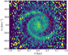 |
Fig. 4 Two-armed phase spiral in the region 1400 < LZ/kpc km s−1 < 1500, d < 1 kpc, 175° < θϕ < 185°. The area that both spiral arms appear to emerge from is marked with a red ellipse. |
3.2 Location of the two-armed phase spiral
Figure 4 shows the two-armed phase spiral in number density contrast with a Gaussian filter for stars in the solar neighbourhood with low angular momentum, LZ = 1450 ± 50 kpc km s−1. This plot establishes some characteristics of the two-armed phase spiral. Mainly that it appears similar to the one-armed phase spiral seen at higher angular momentum but with an extra arm emerging from the same “root” as the first one (marked with a red ellipse) but winding slower and ending before it would cross into the negative Z-range.
Figure 5 shows the stellar number density contrast in multiple regions of R and LZ. We can see that the two-armed phase spiral only appears in a limited region around panel g, with R ≈ 8 kpc and LZ ≈ 1450 kpc km s−1. We also see a one-armed phase spiral at higher angular momentum in Figs. 5b and 5c, and at the same or lower angular momentum in Figs. 5o and 5p.
In Fig. 6, we see the same sample of stars coloured by mean galactocentric radial velocity. Here we see a two-armed spiral pattern in the middle two rows, between 1400 and 1600 kpc km s−1. Since the mean radial velocity is much less affected by dust, this is a useful method for tracing phase spirals (Li et al. 2023).
Figure 7 shows the same regions as Fig. 5 but coloured by mean metallicity. Here we can see two faint ridges corresponding to a two-armed spiral pattern (Fig. 7g), the same panel that shows the strongest pattern in Fig. 5. This indicates that the stars participating in the two-armed phase spiral are of a slightly higher mean metallicity than others at the same vertical energy, at the same distance from the centre of phase space. This suggests that these stars have been transported from a region of space or phase space with higher mean metallicity. Given the well-known vertical and radial gradients in metallicity (e.g. Recio-Blanco et al. 2023), they may have been scattered from an original location at a lower galactocentric radius or a lower amplitude vertical oscillation (or both) by one of the mechanisms that form phase spirals.
Free parameters in the model of the phase spiral.
3.3 The two-armed model
We used a model to quantify the properties of the two-armed phase spiral. The model used a Markov Chain Monte Carlo approach to fit a mathematical spiral defined by
![Mathematical equation: $\[r=b \phi_s+c \phi_s^2\]$](/articles/aa/full_html/2024/10/aa51387-24/aa51387-24-eq7.png) (1)
(1)
to a 2D histogram of an observed phase spiral in phase space. The model created a smooth background of the phase space distribution of stars which removed all the detailed features of the distribution, including the arms of the phase spiral. The model then tried to find a set of parameters for a mathematical spiral such that when it was multiplied with the smooth background, it recreated the original distribution. The model used the scale factor S to measure the axis ratio of the phase spiral. It worked by stretching the VZ axis such that a higher scale factor increases the vertical velocity extent of the phase spiral. This was needed as the phase spiral is known to change shape, especially with galactocentric radius (e.g. Laporte et al. 2019; Li 2021), and the scale factor accounted for this in the model. This was done by changing the way distances and angles were computed in the following equations,
![Mathematical equation: $\[r=r\left(Z, V_Z\right)=\sqrt{Z^2+\left(\frac{V_Z}{S}\right)^2} \text {, }\]$](/articles/aa/full_html/2024/10/aa51387-24/aa51387-24-eq8.png) (2)
(2)
![Mathematical equation: $\[\theta=\theta\left(Z, V_Z\right)=\arctan \left(\frac{1}{S} \frac{V_Z}{Z}\right).\]$](/articles/aa/full_html/2024/10/aa51387-24/aa51387-24-eq9.png) (3)
(3)
For the full equation for the phase spiral, we took inspiration from Widmark et al. (2021) and ended up with
![Mathematical equation: $\[f(r, \theta)=1+\alpha \cdot \operatorname{sigm}\left(\frac{r-\rho}{0.1 \mathrm{~kpc}}\right) \cos \left(\theta-\phi_s(r)-\theta_0\right).\]$](/articles/aa/full_html/2024/10/aa51387-24/aa51387-24-eq10.png) (4)
(4)
All free parameters are named in Table 1 and ϕs, r, and θ are defined in Eqs. (1), (2), and (3) respectively. For a full and detailed description of the model and all parameters, see Alinder et al. (2023) where it was initially developed.
The model used in this paper was modified to consist of two independent phase spirals combined together after we applied a Gaussian filter to the phase plane. The parameters of each of the two phase spirals can be extracted separately. When the modified model compared the mathematical spiral to the phase space distribution, instead of making the comparison right away, it created two spirals and combined them using an elementwise maximum function. Rather than attempting to fit these spirals to the normal number density distribution, the modified model attempted to match the spirals to the distribution after it had been processed with a Gaussian filter. This filter used a kernel size that corresponds to 500 pc in the Z direction and 40 km s−1 in the VZ direction, and has had noise suppressed by clipping pixels with values smaller than the 5th percentile or larger than the 95th percentile.
We also wanted to be able to measure the rotation of the phase spiral with this model. The model parameter θ0 represented the angle offset, which is the rotation of the phase spiral in the model. However, this parameter was not a convenient descriptor of the phase spiral’s rotation because it had a degeneracy with the linear winding parameter b, and also to a certain extent with the quadratic winding parameter c. Different sets of these values could produce very similar spirals except in the most central regions, which were softened through the flattening parameter. Therefore, we described the rotation of the phase spiral by measuring the angle of the spiral arm at a fixed phase distance. These angles are shown in Fig. 8 with red lines, and the phase distance the measurements were made at is indicated with a white ring (scaled to the same axis ratio as the phase spirals) in the lower row. The angle 0° is shown with a dashed white line in the upper row. Changing the phase distance at which we take these measurements does not change our results significantly except by changing all angles by a constant amount.
The model used in this paper had slightly different allowed parameter ranges than the one used in Alinder et al. (2023), and these are listed in Table 1. These changes allowed the model to find a tighter phase spiral by reducing the two winding parameters and making it pay more attention to the inner part of the phase spiral by reducing the maximum flattening distance. The winding parameters specified how tightly the phase spiral turned with radial distance. The flattening distance ρ is the size of an area in the centre of the phase plane where the spiral function is “flattened” to reduce the significance of the central region since it is not fitted well by this kind of model. If these changes were not made, the model may have explored solutions with very tight spirals (large values of the winding parameters in Eq. (1)) and got stuck in false minima with unreasonable solutions. The changes were:
b was changed to the range 0.005–0.1 from 0.01–0.175,
max c was reduced to 0.004 from 0.005,
Max flattening distance was reduced to 0.18 from 0.3.
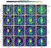 |
Fig. 5 Z-VZ phase plane at different radii (left to right) and angular momenta (top to bottom), showing the one- or two-armed phase spiral. In all cases, the data are restricted to 170° < θϕ < 190°. The quantity indicated by the colour bar is the number density contrast after processing with our Gaussian filter. |
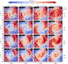 |
Fig. 6 Z–VZ phase plane coloured by galactocentric radial velocity. Individual plots are at different radii (left to right) and angular momenta (top to bottom). In all cases, the data are restricted to 170° < θϕ < 190°. |
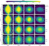 |
Fig. 7 Two-armed phase spiral at different locations, coloured by mean metallicity. In panel g, we can see a trace of a spiral arm in the negative z, positive vz quadrant. |
3.4 Rotation
In Alinder et al. (2023), we investigated how the phase spiral changes with azimuthal angle and found that the phase spiral in the outer Galactic disc rotates with azimuthal angle ϕ at a rate of about 3° per degree of ϕ. This region is an angular momentum range of 2200 < LZ/kpc km s−1 < 2400 and a galactocentric radial range of 8.5 < R/kpc < 10.5. In this study, we use the phase angle θϕ, instead of the azimuthal angle ϕ, when selecting stars. To ensure the results of this paper are comparable with those of Alinder et al. (2023), we plot the phase spiral in the outer Galactic disc using both ϕ and θϕ. Figure 9 shows the phase spiral in the outer Galactic disc at different values of ϕ (left column) and θϕ (right column). An animated version of this comparison can be seen online3. The figure shows a comparison of the phase spiral plotted using stars in three different ranges of phase angle θϕ or azimuthal angle ϕ values. The general appearance and rotational behaviour of the phase spiral are similar in both columns. Both columns of the figure show the clearly identifiable phase spiral in the outer Galactic disc rotating approximately half a rotation over the shown range of angles. The phase spiral plotted using ϕ appears to be more strongly affected by dust at high and low angles as there is a noticeable decrease in the number density of stars around Z = 0 pc. This effect is present but much weaker in the phase spiral drawn using θϕ, as not all stars in the frames with high or low angles are physically distant from the Sun.
We want to compare the rotation of the one-armed phase spiral in the outer Galactic disc, seen in Fig. 9, with the rotation of the two-armed phase spiral as seen in the angular momentum range of 1400 < LZ/kpc km s−1 < 1500 in the solar neighbourhood, as illustrated in Fig. 10. In order to do so we plotted the number density contrast of the phase plane of stars in this angular momentum range and within 1 kpc of the Sun in a 5° slice around 180° in both ϕ and θϕ, shown in Fig. 114. The left panel is plotted using θϕ. In it, both arms of the phase spiral can be seen while in the right panel, plotted using ϕ, the spiral pattern is much less clear but still vaguely detectable. Since the phase spiral in this region rotates with θϕ, and the phase spiral in the outer Galactic disc rotates with both ϕ and θϕ, it is reasonable to assume the reason for this rotation is similar or the same in the two regions.
In Fig. 10, we can see how the phase spiral changes with θϕ angle. The figure shows the number density contrast with a range of θϕ going from 195° to 165° with each panel covering 10°. Both arms of the phase spiral can be seen to rotate and the range of rotation is approximately 90° over this range of θϕ. The phase spiral rotates clockwise with decreasing θϕ, similar to the phase spirals observed in Alinder et al. (2023).
Now we employ our model, discussed in Sect. 3.3, to fit the two-armed phase spiral. We wanted to measure how the phase angle θϕ affects the rotation of the phase spiral and we wanted to measure the difference in angle between the two spirals over a range of phase angles. In Fig. 12, we can see the results of the model. In the upper panel, we see two tracks. These two tracks are the orientation of the two arms of the phase spiral, called Spiral angle in the figure, as identified by our model. Over the range of θϕ = 160° to θϕ = 200°, the arms of the phase spiral move from a spiral angle of approximately 0° to 90° and −180° to −90° respectively. The bottom panel shows the difference in spiral angle between the two arms. The distance stays mostly consistent but a least-squares fitted line reveals that the separation is increasing at a rate of about 0.5° in Δ spiral angle per 1° in θϕ in this range.
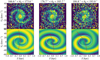 |
Fig. 8 Visualisation of how the angle of the arms of the phase spiral is found. Upper row: number density contrast of the two-armed phase spiral at low, medium, and high θϕ. The spiral angle is marked with a red line and the zero-point for the angle is a dashed white line. Lower row: model of the two-armed phase spiral corresponding to the data in the top row. The spiral angle and measurement distance are marked with a red line and a white ring respectively. |
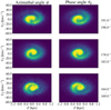 |
Fig. 9 Comparison of the normalised number density phase spiral in the outer Galactic disc sliced by azimuthal angle and phase angle. An animated version is available online. |
3.5 Axis ratio
In Fig. 10, the phase spiral also appears to change shape, becoming less extended in the Z-direction and more extended in the VZ-direction. The axis ratio is parametrised in the model with the scale factor S, so it can be examined in the same way as the rotation angle above. Figure 13 shows the values for the scale factor for the same model run seen in Fig. 12. The figure shows a distribution with a large spread but a clear peak at around θϕ = 175°. It is unclear to us whether the ~10 points marked by the red ellipse at θϕ > 190° above the main line are spurious, due to large uncertainties, or indicate a genuine increase in scale factor in this region.
This dependence of the axis ratio on a spacial location has been seen previously by, for instance, Widmark et al. (2022) and Guo et al. (2024) and is usually taken to be a probe of the vertical potential of the disc. Assuming this is the case, we encourage future studies into how to use the varying shape of the two-armed phase spiral to investigate azimuthal differences in the potential of the galactic disc.
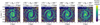 |
Fig. 10 Number density contrast in the phase plane showing the two-armed phase spiral at different values of θϕ. The stars are in the angular momentum range of 1400–1500 kpc km s−1 and at a galactocentric distance of 7.5 kpc to 8 kpc. The phase spiral appears to rotate counter-clockwise with increasing phase angle. The data presented in this figure can also be seen as an animation online. |
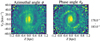 |
Fig. 11 Comparison of the two-armed phase spiral with stars selected using azimuthal angle ϕ, left, and phase angle θϕ, right, both in the range from 178° to 183°. The right panel shows a relatively clear two-armed phase spiral, while it is relatively faint in the left panel. An animated version of this figure is available online. |
4 Discussion
Vertical disturbances of the Milky Way’s disc have been a subject of research for several decades. The warp of the Galactic disc has been recognised since Kerr (1957) found it in the gas component and Freudenreich et al. (1994) in the stellar component, showing that the Galactic disc is not a simple, flat structure.
With the data made available by the Gaia mission, a much fuller view of the complexities of the structures in the Galactic disc has been revealed, with numerous studies investigating different views of the Galactic disc’s disturbances. Poggio et al. (2018) map the warp in populations of both young and old stars out to 7 kpc from the Sun. Antoja et al. (2018) find the signal of the warp as a vertical velocity gradient in both populations in the outer Galactic disc and claim this supports the hypothesis that the warp is a gravitationally induced phenomenon. Ramos et al. (2018) find numerous ridges in Vϕ − R space and suggest the various structures they see may be the results of several different mechanisms acting on the disc. Thulasidharan et al. (2022) compare the motions of young and old stars close to the Radcliffe Wave (Alves et al. 2020) and find that the young stars show a possible association with the wave whereas the old population does not. Their analysis indicates that the vertical oscillations of the stellar population extend beyond the Radcliffe Wave, suggesting it is part of a larger disc mode induced by an external perturber such as the Sagittarius dwarf galaxy. Gaia Collaboration (2021b) investigate the velocity distribution of stars in the outer Galactic disc and find it asymmetric with respect to the plane of the Galaxy. They also find the VZ−Vϕ distribution to be bimodal, forming two clumps, as well as additional ridges in Vϕ−R space. Hunt et al. (2024) find traces of phase spirals in R-VR space in the solar neighbourhood which may have a different origin than the Z−VZ phase spirals discussed in this paper. Cao et al. (2024) look at waves in the LZ − ⟨VR⟩ space which they suggest has an origin that is internal to the Galaxy, and may possibly be useful for inferring information about the properties of the bar. It seems likely that many of these phenomena have the same root cause, and that what we are really observing are different facets of a grand and complicated dynamical system. These connections present a rich vein of potential research, but a closer investigation of them is beyond the scope of this paper. A deeper study of these relations will be possible with data from large spectroscopic surveys such as 4MIDABLE-HR (4MOST MIlky way Disc And BuLgE High-Resolution) Bensby et al. (2019) and 4MIDABLE-LR (4MOST MIlky way Disk And BuLgE Low-Resolution Survey) Chiappini et al. (2019) that will provide detailed elemental abundances and ages for millions of stars throughout the Milky Way disc.
It is reasonable to assume that the properties of the two-armed phase spiral can, in some way, be related to its formation. It is unclear why the phase spiral has two arms in just the specific range found in this investigation and not elsewhere. It might be because the formation mechanism results in a weak two-armed pattern, that the two-armed phase spiral used to exist across a large range but has been attenuated over time, or that the mechanism works strongest in a different region of the Galaxy and we are only detecting the edges of the stronger pattern produced by that mechanism. The last option seems unlikely as it would imply that it should be possible to detect a stronger signal by looking in a different, presumably adjacent, region, which has been attempted in this paper without success in Sect. 3.
Hunt et al. (2022) argue that the two-armed phase spiral is a response to a “breathing mode”, that is, compression and rarefaction of stars vertically in the Galactic disc. This response has been found in theoretical calculations by Banik et al. (2022) and in N-body simulations by Hunt et al. (2021). As Hunt et al. (2022) note, the most likely way to produce this in the inner part of the Galactic disc is by internal perturbations, rather than the response to an interaction with a satellite galaxy. If this is indeed the case, possibly due to strong spiral arms within the disc, it would suggest the two-armed phase spiral is a rather localised effect. If the two-armed phase spiral indeed has a different origin from the one-armed phase spiral, that might account for some of the differences in observed properties.
Widmark et al. (2021) use the structure and shape of the one-armed phase spiral to infer the gravitational potential of the Milky Way disc. This intuitively fits with the observed increase in the vertical velocity range of the phase spiral with increased galactocentric radial distance (e.g. Li 2021). The change in axis ratio with phase angle illustrated in Figs. 10 and 13 would therefore appear to indicate that there is also a change in Galactic disc potential with azimuthal angle (corresponding to phase angle). This can happen due to the spiral arms, but it would certainly appear that the variation with phase angle that we see is too large to be simply explained by this. A crude estimate of the relation of our axis ratio to the gravitational potential would note that this axis ratio is likely to be proportional to the vertical orbital frequencies, such as the vertical epicycle frequency, and that these are proportional to the square root of the potential gradient, and therefore roughly proportional to the square root of the surface density. The variation in axis ratio we observe would therefore imply surface density variations of at least an order of 50%, which are well beyond those that we believe occur due to the Milky Way’s spiral arms. It would appear that efforts to constrain the Milky Way’s surface density using the two-armed phase spiral will need a more careful understanding of their formation mechanism and propagation through the Galactic disc.
The result that the two-armed phase spiral is visible in mean metallicity data is consistent with the basic picture of phase spiral production. A phase spiral is believed to be created when stars in the Galactic disc are acted on by a force, creating an initially synchronised vertical motion. The stars that have been so displaced will have angular frequencies depending on the extent of their vertical motion such that those with the smallest excursions will oscillate about the midplane with the highest frequency. This naturally creates a spiral pattern when viewed in Z − VZ space. The stars that are part of the phase spiral have therefore been moved out of the midplane of the Galactic disc and the central region of phase space to live in the outer parts of the phase plane. The stars that otherwise exist in this part of phase space are more likely to be those belonging to the Galactic thick disc and are therefore expected to have lower mean metallicity (Bensby et al. 2014).
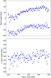 |
Fig. 12 Measurement of phase angle for phase spirals at different azimuthal angles of guiding centre θϕ. Top panel: rotation angle of the phase spirals as functions of θϕ for stars in the solar neighbourhood (d < 1 kpc). Each point uses data from ±3.5°. The zero point of the spiral angle is arbitrary. Bottom panel: difference in the angle of the arms of the phase spiral. The trend is fitted with a line. |
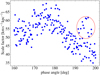 |
Fig. 13 Scale factor of the model as a function of phase angle θϕ. The scale factor is equivalent to the axis ratio of the phase spiral. The scale factor shows a peak at around θϕ = 175°. The points contained by the red ellipse are off the apparent sequence, and it is unclear whether to attribute them to difficulties fitting the phase spirals in that region or a genuine increase in scale factor. |
5 Summary and conclusions
In this study, we use astrometric and line-of-sight velocity data from Gaia DR3 and stellar metallicities derived by Andrae et al. (2023) from Gaia XP spectra to investigate and characterise the properties of the two-armed phase spiral in the solar neighbourhood. We compute action-angle variables for these stars and use the azimuthal angle of the guiding centre or phase angle (θϕ) when selecting stars, rather than the azimuthal position of the star (ϕ). This reveals clearer spiral patterns in phase space. A Gaussian filtering technique further enhances the contrast of the phase spiral in the plots.
The properties of the two-armed phase spiral are quantified using a model that fits a mathematical spiral to the observed phase space distribution of stars. The model incorporates parameters capturing the different aspects of the shape of the phase spiral including one, S, to account for the changes in axis-ratio. This model is a version of the model we developed in Alinder et al. (2023), modified to fit two spiral arms rather than one.
We find that it is only in a narrow range of angular momentum (≈1400–1500 kpc km s−1) in the solar neighbourhood, that the phase spiral has two arms. At both higher and lower angular momentum, the phase spiral has one arm. This two-armed phase spiral is a faint structure that is easiest to detect in this narrow range of low angular momentum and with a phase angle θϕ near 180°.
We are able to show that the two-armed phase spiral rotates with phase-angle around the Galaxy, changing by about 2.25° per degree of θϕ. This is similar behaviour to the one-armed phase spiral in the outer Galactic disc which rotates as described in Alinder et al. (2023) with either azimuthal angle ϕ or phase angle θϕ. The difference in angle of the two arms of the two-armed phase spiral appears to increase by about 0.5° per degree of θϕ. We are also able to see that the axis ratio of the two-armed phase spiral varies with θϕ in a similar manner to how the axis ratio of one-armed phase spirals varies with galactocentric distance.
We show that the stars in the overdense regions of phasespace associated with the two-armed phase spiral have a slightly higher mean metallicity than those with equivalent vertical oscillations. This is likely to be because they were scattered from, for example, orbits nearer the Galactic plane.
The two-armed phase spiral remains a complicated and poorly understood phenomenon. Understanding why it is restricted to a relatively small range in angular momentum, and why it varies in shape substantially across the phase angles we are able to study, may offer us an insight into the structure and history of this region of the Galaxy where dynamical perturbations can be expected to be dominated by the Milky Way’s spiral arms.
Data availability
Movies associated to Figs 9, 10, 11 are available at https://www.aanda.org
Acknowledgements
PM gratefully acknowledges support from a project grant from the Swedish Research Council (Vetenskaprådet, Reg: 2021-04153). TB and SA acknowledge support from project grant No. 2018-04857 from the Swedish Research Council. Some of the computations in this project were completed on computing equipment bought with a grant from The Royal Physiographic Society in Lund. This work has made use of data from the European Space Agency (ESA) mission Gaia (https://www.cosmos.esa.int/gaia), processed by the Gaia Data Processing and Analysis Consortium (DPAC, https://www.cosmos.esa.int/web/gaia/dpac/consortium). Funding for the DPAC has been provided by national institutions, in particular the institutions participating in the Gaia Multilateral Agreement. This research has made use of NASA’s Astrophysics Data System. This work made use of the following software packages for Python, AstroPy (Astropy Collaboration 2022), emcee Foreman-Mackey et al. (2013), Numpy (Harris et al. 2020), Matplotlib (Hunter 2007), SciPy (Virtanen et al. 2020).
References
- Alinder, S., McMillan, P. J., & Bensby, T. 2023, A&A, 678, A46 [NASA ADS] [CrossRef] [EDP Sciences] [Google Scholar]
- Alves, J., Zucker, C., Goodman, A. A., et al. 2020, Nature, 578, 237 [NASA ADS] [CrossRef] [Google Scholar]
- Andrae, R., Rix, H.-W., & Chandra, V. 2023, ApJS, 267, 8 [NASA ADS] [CrossRef] [Google Scholar]
- Antoja, T., Helmi, A., Romero-Gómez, M., et al. 2018, Nature, 561, 360 [Google Scholar]
- Antoja, T., Ramos, P., García-Conde, B., et al. 2023, A&A, 673, A115 [NASA ADS] [CrossRef] [EDP Sciences] [Google Scholar]
- Astropy Collaboration (Price-Whelan, A. M., et al.) 2022, ApJ, 935, 167 [NASA ADS] [CrossRef] [Google Scholar]
- Bailer-Jones, C. A. L., Rybizki, J., Fouesneau, M., Demleitner, M., & Andrae, R. 2021, AJ, 161, 147 [Google Scholar]
- Banik, U., Weinberg, M. D., & van den Bosch, F. C. 2022, ApJ, 935, 135 [NASA ADS] [CrossRef] [Google Scholar]
- Bennett, M., & Bovy, J. 2019, MNRAS, 482, 1417 [NASA ADS] [CrossRef] [Google Scholar]
- Bennett, M., Bovy, J., & Hunt, J. A. S. 2022, ApJ, 927, 131 [NASA ADS] [CrossRef] [Google Scholar]
- Bensby, T., Feltzing, S., & Oey, M. S. 2014, A&A, 562, A71 [NASA ADS] [CrossRef] [EDP Sciences] [Google Scholar]
- Bensby, T., Bergemann, M., Rybizki, J., et al. 2019, The Messenger, 175, 35 [NASA ADS] [Google Scholar]
- Binney, J., & Schönrich, R. 2018, MNRAS, 481, 1501 [Google Scholar]
- Binney, J., & Tremaine, S. 2008, Galactic Dynamics: Second Edition (Princeton, NJ, USA: Princeton University Press) [Google Scholar]
- Bland-Hawthorn, J., Sharma, S., Tepper-Garcia, T., et al. 2019, MNRAS, 486, 1167 [NASA ADS] [CrossRef] [Google Scholar]
- Cao, C., Li, Z.-Y., Schönrich, R., & Antoja, T. 2024, arXiv e-prints [arXiv:2403.14953] [Google Scholar]
- Chiappini, C., Minchev, I., Starkenburg, E., et al. 2019, The Messenger, 175, 30 [NASA ADS] [Google Scholar]
- Drimmel, R., & Poggio, E. 2018, RNAAS, 2, 210 [NASA ADS] [Google Scholar]
- Foreman-Mackey, D., Hogg, D. W., Lang, D., & Goodman, J. 2013, PASP, 125, 306 [Google Scholar]
- Frankel, N., Bovy, J., Tremaine, S., & Hogg, D. W. 2023, MNRAS, 521, 5917 [NASA ADS] [CrossRef] [Google Scholar]
- Freudenreich, H. T., Berriman, G. B., Dwek, E., et al. 1994, ApJ, 429, L69 [NASA ADS] [CrossRef] [Google Scholar]
- Gaia Collaboration (Brown, A. G. A., et al.) 2016a, A&A, 595, A2 [NASA ADS] [CrossRef] [EDP Sciences] [Google Scholar]
- Gaia Collaboration (Prusti, T., et al.) 2016b, A&A, 595, A1 [NASA ADS] [CrossRef] [EDP Sciences] [Google Scholar]
- Gaia Collaboration (Brown, A. G. A., et al.) 2018, A&A, 616, A1 [NASA ADS] [CrossRef] [EDP Sciences] [Google Scholar]
- Gaia Collaboration (Antoja, T., et al.) 2021a, A&A, 649, A8 [EDP Sciences] [Google Scholar]
- Gaia Collaboration (Brown, A. G. A., et al.) 2021b, A&A, 649, A1 [NASA ADS] [CrossRef] [EDP Sciences] [Google Scholar]
- Gaia Collaboration (Drimmel, R., et al.) 2023, A&A, 674, A37 [CrossRef] [EDP Sciences] [Google Scholar]
- Grand, R. J. J., Pakmor, R., Fragkoudi, F., et al. 2023, MNRAS, 524, 801 [NASA ADS] [CrossRef] [Google Scholar]
- GRAVITY Collaboration (Abuter, R., et al.) 2018, A&A, 615, A15 [CrossRef] [EDP Sciences] [Google Scholar]
- Guo, R., Li, Z.-Y., Shen, J., Mao, S., & Liu, C. 2024, ApJ, 960, 133 [NASA ADS] [CrossRef] [Google Scholar]
- Harris, C. R., Millman, K. J., van der Walt, S. J., et al. 2020, Nature, 585, 357 [NASA ADS] [CrossRef] [Google Scholar]
- Hunt, J. A. S., Stelea, I. A., Johnston, K. V., et al. 2021, MNRAS, 508, 1459 [NASA ADS] [CrossRef] [Google Scholar]
- Hunt, J. A. S., Price-Whelan, A. M., Johnston, K. V., & Darragh-Ford, E. 2022, MNRAS, 516, L7 [NASA ADS] [CrossRef] [Google Scholar]
- Hunt, J. A. S., Price-Whelan, A. M., Johnston, K. V., et al. 2024, MNRAS, 527, 11393 [Google Scholar]
- Hunter, J. D. 2007, Comput. Sci. Eng., 9, 90 [NASA ADS] [CrossRef] [Google Scholar]
- Kerr, F. J. 1957, AJ, 62, 93 [NASA ADS] [CrossRef] [Google Scholar]
- Laporte, C. F. P., Minchev, I., Johnston, K. V., & Gómez, F. A. 2019, MNRAS, 485, 3134 [Google Scholar]
- Li, Z.-Y. 2021, ApJ, 911, 107 [NASA ADS] [CrossRef] [Google Scholar]
- Li, C., Siebert, A., Monari, G., Famaey, B., & Rozier, S. 2023, MNRAS, 524, 6331 [NASA ADS] [CrossRef] [Google Scholar]
- Lindblad, B. 1941, Stockholms Observatoriums Ann., 13, 10.1 [NASA ADS] [Google Scholar]
- McMillan, P. J. 2017, MNRAS, 465, 76 [NASA ADS] [CrossRef] [Google Scholar]
- Poggio, E., Drimmel, R., Lattanzi, M. G., et al. 2018, MNRAS, 481, L21 [Google Scholar]
- Ramos, P., Antoja, T., & Figueras, F. 2018, A&A, 619, A72 [NASA ADS] [CrossRef] [EDP Sciences] [Google Scholar]
- Recio-Blanco, A., de Laverny, P., Palicio, P. A., et al. 2023, A&A, 674, A29 [NASA ADS] [CrossRef] [EDP Sciences] [Google Scholar]
- Reid, M. J., & Brunthaler, A. 2004, ApJ, 616, 872 [Google Scholar]
- Sellwood, J. A., & Binney, J. J. 2002, MNRAS, 336, 785 [Google Scholar]
- Thulasidharan, L., D’Onghia, E., Poggio, E., et al. 2022, A&A, 660, L12 [NASA ADS] [CrossRef] [EDP Sciences] [Google Scholar]
- Tremaine, S., Frankel, N., & Bovy, J. 2023, MNRAS, 521, 114 [NASA ADS] [CrossRef] [Google Scholar]
- Vasiliev, E. 2019, MNRAS, 482, 1525 [Google Scholar]
- Virtanen, P., Gommers, R., Oliphant, T. E., et al. 2020, Nature Methods, 17, 261 [CrossRef] [Google Scholar]
- White, S. D. M., & Rees, M. J. 1978, MNRAS, 183, 341 [Google Scholar]
- Widmark, A., Laporte, C., & de Salas, P. F. 2021, A&A, 650, A124 [NASA ADS] [CrossRef] [EDP Sciences] [Google Scholar]
- Widmark, A., Laporte, C. F. P., & Monari, G. 2022, A&A, 663, A15 [NASA ADS] [CrossRef] [EDP Sciences] [Google Scholar]
- Widrow, L. M. 2023, MNRAS, 522, 477 [NASA ADS] [CrossRef] [Google Scholar]
The galactocentric coordinate system used in this study places the Sun on the negative X-axis (ϕ = 180°) at a distance of 8.122 kpc and a height of 20.8 pc, with the Y-axis in the same direction as l = 90°, and the Z-axis is in the same direction as b = 90°. Galactic azimuth, ϕ, decreases in the direction of Galactic rotation, and the Sun has velocity components VR,⊙ = −12.9, Vϕ,⊙ = −245.6, VZ,⊙ = −7.78 km s−1. (Reid & Brunthaler 2004; Drimmel & Poggio 2018; GRAVITY Collaboration 2018; Bennett & Bovy 2019). For the computations and definitions of coordinates, we use Astropy v5.2 (Astropy Collaboration 2022).
The animation covers 210° to 150°. The frames have large overlaps with each frame covering 5°.
This comparison is also available as an animation online. The animation shows the number density contrast from ϕ and θϕ in the range 200° to 160° with each frame covering 5°. The rotation seen in θϕ is approximately 90° over this range. In ϕ, a phase spiral can only barely be seen in the densest part, around ϕ = 180°, but a rotation is hard to discern.
All Tables
All Figures
|
Fig. 1 Comparison of |
| In the text | |
|
Fig. 2 Comparison of phase spiral clarity when selecting stars based on azimuthal angle (ϕ, left column) and azimuthal angle of the guiding centre or phase angle (θϕ, right column), and using a Gaussian filter (bottom row) compared to not using one (top row). We can note that the right column, particularly the bottom row, has a much clearer spiral pattern than the rest. The plots show number density and number density contrast in the Z − VZ phase plane of stars in the solar neighbourhood (d < 1 kpc) with a further selection by ϕ or θϕ. The left column shows stars with 175° < ϕ < 185° and the right column shows stars with 175° < θϕ < 185°. All stars have 1400 < LZ/kpc km s−1 < 1500. |
| In the text | |
|
Fig. 3 Comparison of the distributions of azimuthal angle ϕ and azimuthal angle of guiding centre θϕ for stars in the solar neighbourhood (d < 1 kpc). |
| In the text | |
|
Fig. 4 Two-armed phase spiral in the region 1400 < LZ/kpc km s−1 < 1500, d < 1 kpc, 175° < θϕ < 185°. The area that both spiral arms appear to emerge from is marked with a red ellipse. |
| In the text | |
|
Fig. 5 Z-VZ phase plane at different radii (left to right) and angular momenta (top to bottom), showing the one- or two-armed phase spiral. In all cases, the data are restricted to 170° < θϕ < 190°. The quantity indicated by the colour bar is the number density contrast after processing with our Gaussian filter. |
| In the text | |
|
Fig. 6 Z–VZ phase plane coloured by galactocentric radial velocity. Individual plots are at different radii (left to right) and angular momenta (top to bottom). In all cases, the data are restricted to 170° < θϕ < 190°. |
| In the text | |
|
Fig. 7 Two-armed phase spiral at different locations, coloured by mean metallicity. In panel g, we can see a trace of a spiral arm in the negative z, positive vz quadrant. |
| In the text | |
|
Fig. 8 Visualisation of how the angle of the arms of the phase spiral is found. Upper row: number density contrast of the two-armed phase spiral at low, medium, and high θϕ. The spiral angle is marked with a red line and the zero-point for the angle is a dashed white line. Lower row: model of the two-armed phase spiral corresponding to the data in the top row. The spiral angle and measurement distance are marked with a red line and a white ring respectively. |
| In the text | |
|
Fig. 9 Comparison of the normalised number density phase spiral in the outer Galactic disc sliced by azimuthal angle and phase angle. An animated version is available online. |
| In the text | |
|
Fig. 10 Number density contrast in the phase plane showing the two-armed phase spiral at different values of θϕ. The stars are in the angular momentum range of 1400–1500 kpc km s−1 and at a galactocentric distance of 7.5 kpc to 8 kpc. The phase spiral appears to rotate counter-clockwise with increasing phase angle. The data presented in this figure can also be seen as an animation online. |
| In the text | |
|
Fig. 11 Comparison of the two-armed phase spiral with stars selected using azimuthal angle ϕ, left, and phase angle θϕ, right, both in the range from 178° to 183°. The right panel shows a relatively clear two-armed phase spiral, while it is relatively faint in the left panel. An animated version of this figure is available online. |
| In the text | |
|
Fig. 12 Measurement of phase angle for phase spirals at different azimuthal angles of guiding centre θϕ. Top panel: rotation angle of the phase spirals as functions of θϕ for stars in the solar neighbourhood (d < 1 kpc). Each point uses data from ±3.5°. The zero point of the spiral angle is arbitrary. Bottom panel: difference in the angle of the arms of the phase spiral. The trend is fitted with a line. |
| In the text | |
|
Fig. 13 Scale factor of the model as a function of phase angle θϕ. The scale factor is equivalent to the axis ratio of the phase spiral. The scale factor shows a peak at around θϕ = 175°. The points contained by the red ellipse are off the apparent sequence, and it is unclear whether to attribute them to difficulties fitting the phase spirals in that region or a genuine increase in scale factor. |
| In the text | |
Current usage metrics show cumulative count of Article Views (full-text article views including HTML views, PDF and ePub downloads, according to the available data) and Abstracts Views on Vision4Press platform.
Data correspond to usage on the plateform after 2015. The current usage metrics is available 48-96 hours after online publication and is updated daily on week days.
Initial download of the metrics may take a while.