A non-axisymmetric potential for the Milky Way disk

Y. R. Khalil; B. Famaey; G. Monari; M. Bernet; A. Siebert; R. Ibata; G. F. Thomas; P. Ramos; T. Antoja; C. Li; S. Rozier; M. Romero-Gómez

doi:10.1051/0004-6361/202453077

Home

All issues

Volume 699 (July 2025)

A&A, 699 (2025) A263

Full HTML

Open Access

Issue		A&A Volume 699, July 2025


Article Number		A263
Number of page(s)		19
Section		Galactic structure, stellar clusters and populations
DOI		https://doi.org/10.1051/0004-6361/202453077
Published online		16 July 2025

A&A, 699, A263 (2025)

A non-axisymmetric potential for the Milky Way disk

Y. R. Khalil¹^★, B. Famaey¹, G. Monari¹, M. Bernet²^,3^,4, A. Siebert¹, R. Ibata¹, G. F. Thomas⁵^,6, P. Ramos⁷, T. Antoja²^,3^,4, C. Li⁸^,9, S. Rozier¹⁰ and M. Romero-Gómez²^,3^,4

¹ Université de Strasbourg, CNRS UMR 7550, Observatoire astronomique de Strasbourg, 11 rue de l’Université, 67000 Strasbourg, France
² Departament de Física Quàntica i Astrofísica (FQA), Universitat de Barcelona (UB), C Martí i Franquès 1, 08028 Barcelona, Spain
³ Institut de Ciències del Cosmos (ICCUB), Universitat de Barcelona (UB), C Martí i Franquès, 1, 08028 Barcelona, Spain
⁴ Institut d’Estudis Espacials de Catalunya (IEEC), Edifici RDIT, Campus UPC, 08860 Castelldefels, Barcelona, Spain
⁵ Instituto de Astrofísica de Canarias, 38205 La Laguna, Tenerife, Spain
⁶ Universidad de La Laguna, Dpto. Astrofísica, 38206 La Laguna, Tenerife, Spain
⁷ National Astronomical Observatory of Japan, Mitaka-shi, Tokyo 181-8588, Japan
⁸ School of Astronomy and Space Science, Nanjing University, Nanjing 210093, PR China
⁹ Key Laboratory of Modern Astronomy and Astrophysics (Nanjing University), Ministry of Education, Nanjing 210093, PR China
¹⁰ School of Mathematics and Maxwell Institute for Mathematical Sciences, University of Edinburgh, Kings Buildings, Edinburgh EH9 3FD, UK

^★ Corresponding author: yassin.khalil@unistra.fr

Received: 19 November 2024
Accepted: 9 May 2024

Abstract

We provide a purely dynamical global map of the non-axisymmetric structure of the Milky Way disk. For this, we exploited the information contained within the in-plane motions of disk stars from Gaia DR3 to adjust a model of the Galactic potential, including a detailed parametric form for the bar and spiral arms. We explored the parameter space of the non-axisymmetric components with the backward integration method, first adjusting the bar model to selected peaks of the stellar velocity distribution in the solar neighborhood, and then adjusting the amplitude, phase, pitch angle, and pattern speed of spiral arms to the median radial velocity as a function of position within the disk. We checked a posteriori that our solution also qualitatively reproduces various other features of the global non-axisymmetric phase-space distribution, including most moving groups and phase-space ridges, despite those not being primarily used in the adjustment. This fiducial model has a bar with a pattern speed of 37 km s⁻¹ kpc⁻¹ and two spiral modes that are twoarmed and three-armed, respectively. The two-armed spiral mode has a ~25% local contrast surface density and a low pattern speed of 13.1 km s⁻¹ kpc⁻¹, and matches the location of the Crux-Scutum, Local, and Outer arm segments. The three-armed spiral mode has a ~9% local contrast density, a slightly higher pattern speed of 16.4 km s⁻¹ kpc⁻¹, and matches the location of the Carina-Sagittarius and Perseus arm segments. The Galactic bar, with a higher pattern speed than both spiral modes, has recently disconnected from those two arms. The fiducial non-axisymmetric potential presented in this paper, reproducing most non-axisymmetric signatures detected in the stellar kinematics of the Milky Way disk, can henceforth be used to confidently integrate orbits within the Galactic plane.

Key words: Galaxy: disk / Galaxy: evolution / Galaxy: general / Galaxy: kinematics and dynamics / Galaxy: structure

© The Authors 2025

Open Access article, published by EDP Sciences, under the terms of the Creative Commons Attribution License (https://creativecommons.org/licenses/by/4.0), which permits unrestricted use, distribution, and reproduction in any medium, provided the original work is properly cited.

This article is published in open access under the Subscribe to Open model. Subscribe to A&A to support open access publication.

1 Introduction

The Gaia mission now provides full 6D phase-space information on the Milky Way (MW) disk for a larger number of stars and over a larger volume than ever before. The second (Gaia Collaboration 2018a), early-third (Gaia Collaboration 2021), and third (DR3, Gaia Collaboration 2023a) data releases of Gaia have represented important milestones in this regard (Hunt & Vasiliev 2025). While stellar vertical motions have revealed a disequilibrium of the Galactic disk (Antoja et al. 2018), possibly related to a subtle interplay between external perturbations and internal non-axisymmetries (e.g., Binney & Schönrich 2018; Laporte et al. 2019; Li et al. 2023; Tremaine et al. 2023; Frankel et al. 2024), the rich information contained solely within the inplane motions of stars (e.g., Gaia Collaboration 2018b, 2023b) has not been fully exploited yet. Indeed, these in-plane motions should - in principle - allow us to get a detailed dynamical mapping of the most important non-axisymmetric structures of the MW disk, namely the Galactic bar and the spiral arms (Lynden-Bell & Kalnajs 1972). However, such a detailed mapping is still lacking. This is the focus of the present study.

The existence of the MW bar was originally hypothesized from the observations of gas kinematics (de Vaucouleurs 1964; Peters 1975; Gerhard & Vietri 1986; Binney et al. 1991) and confirmed from (near-)infrared observations (e.g., Blitz & Spergel 1991; Sellwood 1993; Weiland et al. 1994; Binney et al. 1997) as well as bulge stellar kinematics (e.g., Zhao et al. 1994). It is nowadays clear that a large fraction of stars in the bulge region indeed follow a rotating, barred, boxy/peanut shaped structure connected to an edge-on bar (Bland-Hawthorn & Gerhard 2016), whose pattern speed, Ω_b, is nevertheless still subject to debate. Less than three decades ago, a consensus emerged for a pattern speed in the range Ω_b ~ 50-60 km s⁻¹ kpc⁻¹ from various lines of evidence, such as hydrodynamical simulations comparing the modeled gas flow to observed Galactic CO and HI longitude-velocity diagrams (Fux 1999; Englmaier & Gerhard 1999; Bissantz et al. 2003), the Tremaine & Weinberg (1984) method applied to stars in the inner Galaxy (Debattista et al. 2002), or local stellar kinematics (Dehnen 1999b, 2000; Fux 2001) positioning the Sun marginally beyond the 2:1 outer Lindblad resonance (OLR) of the bar. The latter argument has been supported by numerous subsequent analyses (e.g., Minchev et al. 2007; Quillen et al. 2011; Antoja et al. 2012, 2014; Fragkoudi et al. 2019). On the contrary, parallel research on the density of red clump stars in the disk (Wegg et al. 2015), gas kinematics (Sormani et al. 2015; Li et al. 2016), dynamical modeling of stellar kinematics in the inner Galaxy (Portail et al. 2017), and proper motion data from the VVV survey (e.g., Clarke et al. 2019), including with the Tremaine-Weinberg method (Sanders et al. 2019), have collectively pointed to a revised pattern speed of Ω_b ~ 35-40 km s⁻¹ kpc⁻¹. Pérez-Villegas et al. (2017) and Monari et al. (2019b) subsequently demonstrated that the Galactic model adjusted to bulge stellar kinematics by Portail et al. (2017) could effectively replicate several observed features in the local velocity space (see also Monari et al. 2019a; Binney 2020; D’Onghia & Aguerri 2020; Lucchini et al. 2024). Such a lower bar pattern speed is also consistent with observed overdensities in the stellar halo phase-space (Dillamore et al. 2024) and with the chemistry of the disk (Haywood et al. 2024; Khoperskov et al. 2024). Other intermediate pattern speeds have also been proposed (Hunt & Bovy 2018), as have much lower ones (Horta Darrington et al. 2025), while several studies have concluded that stellar kinematics of the disk alone were not sufficient to break the degeneracy (Trick et al. 2021; Trick 2022; Bernet et al. 2024). However, the kinematics of stars in the bar region itself seem to have converged to Ω_b ~ 35-40 km s⁻¹ kpc⁻¹, although possible sudden variations in the pattern speed are also possible (Hilmi et al. 2020). Finally, a steady decrease in the pattern speed of the bar with time has been tentatively detected (Chiba et al. 2021; Chiba & Schönrich 2021), and could explain some aspects of the vertical disequilibrium of the Galactic disk (Li et al. 2023), and can partially contribute to explaining the presence of metal-poor stars with prograde planar orbits in the solar vicinity (Li et al. 2024; Yuan et al. 2024).

Concerning the location and dynamics of spiral arms of the MW, the present observational situation is even less clear than for the bar. The suggestion that the MW could host spiral arms is certainly as old as the realization that it belongs to the realm of disk galaxies, but, due to extinction, it was not before the work of Morgan et al. (1952) that these arms were identified based on the distribution of HII regions, soon followed by the kinematic analysis of the HI 21-cm line by Oort et al. (1958). Based on the distances to OB associations and HII regions, Georgelin & Georgelin (1976) mapped a four-armed spiral pattern, which has been repeatedly confirmed with young or gaseous tracers (e.g., Urquhart et al. 2014), but not with older and redder ones that should better trace the perturbations in the Galactic potential. Indeed, Drimmel (2000), Drimmel & Spergel (2001), Benjamin et al. (2005), and Churchwell et al. (2009) found with near-infrared and mid-infrared tracers that the MW seemingly hosts two main spiral arms. Collecting data on HII regions and giant molecular clouds, Hou et al. (2009) showed that models of three-armed and four-armed logarithmic spirals could connect those different spiral tracers, as has been reviewed in Shen & Zheng (2020). In summary, it is no exaggeration to say that different tracers and observations are far from converging on parameters describing the positions of each spiral arm segment in the MW disk. The so-called Local arm, for example, has been found by Gaia Collaboration (2023b) and Poggio et al. (2021), tracing young stars, to be more extended - and to have an intermediary pitch angle - compared to Vázquez et al. (2008), in which this arm rather heads outward to the Perseus arm, or to Xu et al. (2021), in which the Local arm heads inward to the Carina-Sagittarius arm. Similar debates exist regarding the Perseus arm and Outer arm with respect to their position in the disk and pitch angle. Perhaps most strikingly, the pitch angle of the Perseus arm has been found to be ~24° in Levine et al. (2006), compatible with the results of Poggio et al. (2021) or Drimmel et al. (2025), and ~9° in Reid et al. (2019), meaning that the name does not actually always refer to the same observed overdensities in the Galactic plane. The situation regarding the pattern speed of spiral arms is even more confused, as its signature can also depend on their dynamical nature and origin (see Sellwood & Masters 2022, for a review). Indeed, numerical simulations of galactic disks offer multiple perspectives on this topic, from transient corotating structures winding up and disappearing quickly (e.g., Baba et al. 2013; Hunt et al. 2018, 2019), to multiple modes persisting over a few (or even many) galactic rotations, falsely appearing as very short-lived due to superposition of modes (e.g., Sellwood & Carlberg 2014). In the following, our modeling procedure will follow two main guidelines. The first guideline is the current consensus that, when spirals appear as modes in simulations, these are not strictly static as in the classical density wave picture (Lin & Shu 1964), but are rather made of a recurrent cycle of groove modes (seeded by a depletion of circular orbits in a narrow range of angular momenta, see, e.g., De Rijcke & Voulis 2016; De Rijcke et al. 2019) that live between their inner Lindblad resonance (ILR) and OLR, where they can create new grooves that set up the recurrent cycle (Sellwood & Carlberg 2014, 2019). They can also be edge modes (Fiteni et al. 2024). The amplitudes of the individual modes grow and decay, but they are nevertheless genuine standing wave oscillations with a fixed shape and pattern speed, detectable over a period of at least one rotation. The second guideline is that spectrograms of N-body simulations displaying joint bar and spiral perturbations tend to display spiral arms that rotate more slowly than the bar; moreover, spiral arms are never present within the corotation radius of the bar. These spirals live between their own ILR and OLR but are usually strongest between their ILR and corotation (Quillen et al. 2011). Our modeling approach does not take into account the possibility of winding spirals with time.

Keeping all the aforementioned caveats in mind, several tentative measurements of the amplitude and pattern speed of spiral arms have been made over time. Originally, Lin et al. (1969) proposed a two-armed model with a pitch angle of 6° and a pattern speed of Ω_s,2 ~ 13 km s⁻¹ kpc⁻¹ based on the systematic motion of gas and the displacement of moderately young stars in their classical density wave model. A more recent estimate based on the classical Lin & Shu (1964) density wave formalism has been made by Siebert et al. (2012) fitting the mean radial velocity map from the RAVE survey and finding a best-fit two-armed spiral model with a contrast surface density of 14%, a pitch angle of 10°, and a pattern speed of Ω_s,2 ~ 18.6 km s⁻¹ kpc⁻¹. This model, however, neglected the effect of the bar (see, e.g., Monari et al. 2014). On the other hand, Amaral & Lepine (1997) argued for a superposition of a two-armed and four-armed spiral, both with a pattern speed of ~20 km s⁻¹ kpc⁻¹ based on tracing back open clusters to their birth place. Such a procedure was recently carried out by Castro-Ginard et al. (2021), who found a declining pattern speed with radius from ~50 km s⁻¹ kpc⁻¹ for the Scutum arm segment to ~17 km s⁻¹ kpc⁻¹ for the Perseus arm segment. Modeling the gas flow in the inner Galaxy, Bissantz et al. (2003) obtained a joint measurement of the bar and four-armed spiral pattern speeds, with a very high pattern speed for the bar, Ω_b ~ 60 km s⁻¹ kpc⁻¹, and a four-armed spiral pattern speed of Ω_s,4 ~ 20 km s⁻¹ kpc⁻¹. More recently, again neglecting the bar, Eilers et al. (2020) applied a toy model of a logarithmic spiral to Gaia DR2 mean Galactocentric radial velocity field to suggest a contrast surface density of ~10%, a pitch angle of 12°, and a fixed pattern speed of Ω_s,2 = 12 km s⁻¹ kpc⁻¹ for a two-armed spiral corresponding to the Local and Outer arms. Such low pattern speeds had also previously been suggested by, for example, Sellwood (2010) based on the signature of a spiral ILR in local stellar kinematics (~8 km s⁻¹ kpc⁻¹ for a two-armed spiral and ~15 km s⁻¹ kpc⁻¹ for a three-armed spiral). Regarding the amplitude, the most recent determination, based on the vertical Jeans equation, has found the Local arm to be the strongest local overdensity, with a contrast density of roughly 20% (Widmark & Naik 2024).

Here, we attempt to fully exploit the rich information encoded within the in-plane stellar motions in Gaia DR3 (Gaia Collaboration 2023b) to dynamically constrain the nonaxisymmetries of the Galaxy. Previous similar attempts include the more empirical approach of Khoperskov et al. (2020); Khoperskov & Gerhard (2022), as well as the recent work of Vislosky et al. (2024) comparing three hydrodynamical simulations of galaxies to the velocity maps from Gaia in order to get insights into the bar-spiral orientation. Our approach hereafter is complementary since, instead of qualitatively comparing a self-consistent hydrodynamical simulation to the data, we attempt a more quantitative fit to the stellar phase-space data from Gaia. For this, we resort to backward integrations to model the velocity field with a parametric form of the gravitational potential. Our preferred solution could serve as the new fiducial non-axisymmetric parametric potential for the MW disk.

In Section 2, we briefly present the data extracted from the RVS sample of Gaia DR3 that we are using to constrain the potential from the MW disk kinematics. The modeling method and the parametrization of the potential are introduced in Section 3, while results are presented in Section 4. A posteriori comparisons with observables to which the model was not fit, as well as some examples of applications of our fiducial potential, are given in Section 5, before our conclusions in Section 6.

2 The Gaia RVS disk sample

Since we were planning to use the in-plane motions of disk stars to constrain the non-axisymmetries of the MW, we selected a sample of stars with 6D phase-space information from the Gaia RVS close to the Galactic plane. We used data from Gaia DR3 (Gaia Collaboration 2023a) combined with the StarHorse (Anders et al. 2022) distances, and selected 17 414 667 stars within a height of 300 pc from the Galactic plane.

We adopted, for the Sun’s position, x_⊙, and velocity, V_⊙, in Galactocentric Cartesian coordinates, x_⊙ = (x_⊙, y_⊙, z_⊙) = (8275, 0, 15.29) pc and V_⊙ = (V_{x_⊙}, V_{y_⊙}, V_{z_⊙}) = (−9.3, 251.5, 8.59) km s⁻¹ (Gaia Collaboration 2023b; Portail et al. 2017; Widmark & Monari 2019), respectively. We then transformed the data from equatorial coordinates to Galactocen-tric coordinates with the Astropy library (Astropy Collaboration 2022) to compute the stars’ positions in Galactocentric Cartesian coordinates, x = (x, y, z), and their in-plane velocities in Galac-tocentric Cylindrical coordinates, V = (V_R, V_φ), with the Galactocentric radius $R = \sqrt{x^{2} + y^{2}}$ $R = \sqrt{x^2 + y^2}$ and azimuth φ = arctan(y/x), defined to be zero at the azimuth of the Sun and positive in the direction of Galactic rotation. The stars were selected within 4kpc < χ < 12 kpc and −4 kpc < y < 4 kpc.

In the left panel of Fig. 1, we display the local stellar velocity distribution for slightly more than 2 million stars within a cylinder of radius 300 pc around the Sun, still within a height of 300 pc. In this figure, several of the well-known moving groups of the solar neighborhood (e.g., Dehnen 1998; Famaey et al. 2005; Antoja et al. 2008; Ramos et al. 2018; Bernet et al. 2022) are immediately visible. The “Hat” can be seen as the downward concave arch at high V_φ, from (V_R, V_φ) ≈ (−100 kms⁻¹, 270 kms⁻¹) to (V_R, V_φ) ≈ (120 kms⁻¹, 260 kms⁻¹). The Sirius moving group (e.g., Famaey et al. 2008) is approximately straight at V_φ ≈ 255 km s⁻¹, located between V_R ≈ −50 km s⁻¹ and V_R ≈ 0 kms⁻¹, with a peak at V_R ≈ −15 kms⁻¹. Coma is right below Sirius in azimuthal velocity, around (V_R, V_φ) ≈ (0 kms⁻¹, 245 km s⁻¹). The Hyades moving group (e.g., Famaey et al. 2007; Pompéia et al. 2011) can be seen as a slightly curved downward arch from the over-density at (V_R, V_φ) ≈ (20 km s⁻¹, 230 km s⁻¹). The Horn is right next to the Hyades, on the other side in V_R : it appears as an arch going through (V_R, V_φ) ≈ (−80 kms⁻¹, 200 kms⁻¹). Finally, the major Hercules moving group is perceived as a bimodality of the whole velocity-plane, with an under-density, just below the Hyades in azimuthal velocity, separating it from the rest of the distribution. Its bimodality appears clearly, with a second overdensity appearing at low V_φ.

Another way to visualize these arches, which, however, visually erases the asymmetries in radial velocity, is to plot the distribution of stars in the local axisymmetric action space (e.g., Trick et al. 2019, 2021). Indeed, the Galaxy is, to leading order, an axisymmetric quasi-integrable system, and the action-angle variables (J, θ) are the canonical phase-space variables appropriate for studying and perturbing integrable systems. In these coordinates, the Hamiltonian only depends on the actions, J, which are integrals of the motion. Each triplet of actions then fully characterizes an integrable orbit, while the angles indicate where a given star is on that particular orbit. The azimuthal action is simply J_φ = RV_φ, while the radial action, J_R (computed within the background axisymmetric potential defined in Sect. 3), encodes the (Galactocentric) radial excursions of a given orbit. In the top right panel of Fig. 1, the arches in the local velocity space are now seen as ridges in the local action space, characteristic of resonant features (e.g., Monari et al. 2017; Binney 2020).

These features of local velocity and action space, traced with exquisite precision, have, however, been known for a long time. The most interesting added value of Gaia data releases has been to expand the volume around the Sun where such dynamical features can be studied (e.g., Ramos et al. 2018; Bernet et al. 2022). In order to adjust the non-axisymmetric components of the Galactic potential, in the present work we, however, refrain from using the full phase-space distribution of disk stars, and instead fit the measure of a central tendency as a function of position in the disk, namely the median Galactocentric radial velocity (Gaia Collaboration 2023b). This map of median radial velocity is displayed in the bottom right panel of Fig. 1 and is the main observable adjusted in the present work. We check only a posteriori the qualitative agreement with the full phase-space distribution of stars. Since our modeling is based on a projected 4D phase-space distribution function (DF, see Sect. 3) of the disk stellar populations - a DF that is supposed to take into account stars with nonzero vertical velocities - we do not make any additional cuts on the vertical velocity in the data. However, while our DF is a projected one, our orbit integrations are performed only within the plane. Therefore, we also checked that selecting only stars with vertical velocities below 15kms⁻¹, allowing us to keep a reasonable number of 11 427 688 stars in the dataset, led to an almost identical median radial velocity map. For the important points of the fit, the typical differences are below 0.5 km/s, with a maximum difference of 1 km/s.

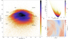Fig. 1

Left panel: 2D histogram of the number density of stars from the Gaia RVS disk sample (in a cylinder of 300 pc radius and ±300 pc height around the Sun) in the (V_R, V_φ) plane defined on a [−200,200] kms⁻¹ × [0,400] kms⁻¹ grid, binned with (1 kms⁻¹)² bins, together with the locations of the different moving groups. Top right panel: Same distribution in the (J_φ, J_R) plane (computed with AGAMA in the potential of Table 1 ) defined on a [0, 600] km s⁻¹ kpc⁻¹ × [200, 3000] km s⁻¹ kpc⁻¹ grid, binned with (3 × 2 km² s⁻² kpc⁻²) bins. Bottom right panel: Median radial velocity V_R (x, y) as a function of the position in the Galactic plane for the full sample of 17 414 667 stars with |z| < 300 pc. The grid is defined as [4, 12] kpc × [−4, 4] kpc, binned with (125 pc)² bins. The Galactic center is located at (x, y) = (0 kpc, 0 kpc), the Sun at (x, y) = (8.275 kpc, 0 kpc) is represented with a cross, and the sense of rotation of the Galaxy is anti-clockwise.

3 Modeling

To build our non-axisymmetric potential, we started from an axisymmetric one, and subsequently added a bar and spiral arms, defined by several parameters as described in the following subsections. Within the axisymmetric potential, we used a phase-space DF, f(x, V), to describe our tracer population. This one-particle DF is the probability density function of finding one star at the phase-space point (x, V) and, for a collisionless system, it obeys the collisionless Boltzmann (or Vlasov) equation. Such a DF, for any steady-state integrable stellar system, should solely be a function of isolating integrals of the motion according to the Jeans theorem (Binney & Tremaine 2008). We take these integrals to be the actions, J. In order to transform stellar positions and velocities into actions, one can use an approximation based on Stäckel potentials (see, e.g., Famaey & Dejonghe 2003). Axisymmetric Stäckel potentials are expressed in a spheroidal coordinate system, defined by a focal distance, which is always related to the first and second derivatives of the potential at any given position. Thus, by using the actual Galactic potential at any given position, one can compute an equivalent focal distance as if the potential were locally of Stäckel form, allowing for the calculation of the (quasi-)integrals of the motion and corresponding actions. This “Stäckel fudge” (Binney 2012; Sanders & Binney 2016) is fully implemented within the actionbased galaxy modeling architecture code (Vasiliev 2018, 2019, AGAMA) that we used in the present study.

We started from an equilibrium DF, f (J), for the tracer population defined within an axisymmetric potential. The first route to include the effect of non-axisymmetric components is to treat them through perturbation theory (e.g., Monari et al. 2016a; Al Kazwini et al. 2022), which, in order to be truly quantitative, needs a special treatment for the resonant zones for a constant pattern speed perturbation (e.g., Monari et al. 2017; Laporte et al. 2020; Binney 2020; Hamilton et al. 2023). This becomes, however, practically very complicated in the presence of multiple perturbers with different pattern speeds, whose resonances will overlap. To circumvent this issue, one can fortunately rely on the property encoded in the collisionless Boltzmann equation, which is that the DF value in an infinitesimal Lagrangian volume is conserved along the trajectory. This allows us to use the classical method of backward integration (Vauterin & Dejonghe 1997) used in, for example, Dehnen (2000); Hunt & Bovy (2018); Hunt et al. (2018, 2019); Monari et al. (2019b); Bernet et al. (2024), in order to explore the shape of the DF.

In order to compute the f (x, V, t), at current time t = 0, at the phase-space point (x, V), in the presence of the bar and spiral arms, we backward-integrated the orbit for a fixed integration time to its phase-space position (x′, V′) at time t′ < 0, before the actual appearance of the non-axisymmetric per-turbers. Assuming that the tracer population is represented by the equilibrium DF, f (J), in the axisymmetric background potential at time t′ , we transformed (x′, V′) to action-angle variables using AGAMA, computed the value of the DF¹, and since this value in an infinitesimal Lagrangian volume is conserved, we attributed the same value of the DF to the phase-space position (x, V) at present time t = 0 in the presence of the bar and spirals. In practice, the orbits were integrated within the plane only, by solving the initial value problem with the Runge-Kutta of the order five method odeint solver from the very efficient torchdiffeq library (Chen 2018) in PyTorch (Paszke et al. 2019). Doing this at numerous phase-space locations allows us to compute the median radial velocity as a function of position in the disk, and to adjust the parameters of the non-axisymmetric components in order to fit the observed values. In practice, the median radial velocity at each grid position (sampled every 50 pc in x and y) on the disk was computed after locally integrating the values of the DF in V_φ for a grid of velocities on which the backward integration was performed at each position. This grid ranges from −79 km s⁻¹ to 79 km s⁻¹ with a step of2 km s⁻¹ in V_R, and from 110 kms⁻¹ to 330 kms⁻¹ with a step of 4 kms⁻¹ in V_ψ. The potential was evaluated on a grid of radii that was subsequently interpolated with a cubic spline in the torchcubicspline library in Pytorch to improve computational time. Similarly, we also interpolated, with Scipy (Virtanen et al. 2020), a cubic spline to the actions computed with AGAMA.

There are three caveats to the method, which are worth mentioning even though addressing them in detail is far beyond the scope of this first quantitative approach to the problem. First, we are using the full disk sample described in the previous section without taking into account a detailed selection function, assuming that the high number of stars that we use allows for a good estimate of the true median velocity. The second caveat is that, in practice, the observed stellar DF is always measured over finite phase-space volumes, while the backward integration method operates under the assumption that the mean value of the DF within a given phase-space volume is equivalent to its value at the central point, irrespective of how the volume deforms during the system’s orbital evolution. In other words, the backward integration method yields the fine-grained DF, which will typically remain unsmoothed at small scales, while the measurable DF within observations is the coarse-grained one, which does not obey the collisionless Boltzmann equation (as this coarsegrained DF is smoothed by phase-mixing within finite volumes). The Nyquist-Shannon sampling theorem imposes limits on the minimum size of fine structures in phase space that can form for a fixed number of particles over time, and this limit is reached on rather short timescales, shorter than collisional relaxation (Beraldo e Silva et al. 2019). Once this limit is reached, the system cannot form finer structures, despite the collisionless Boltzmann equation predicting that these structures do form. In practice, this means that, if the integration is carried out for too long, the fine-grained DF tracked by the backward integration method will lead to sharp and unsmoothed features in velocity space, where chaotic features will also appear as sharper than in the real world. To circumvent this problem, the integration must be carried out only for a relatively limited time, adjusted so that the sharpness of resonant features in velocity space resembles what is observed. Luckily, N-body simulations indicating the existence of recurrent cycles of groove modes in galactic disks (Sellwood & Carlberg 2014, 2019) allow us to consider that current spiral arm modes of the MW are rather recent. This assumption is, of course, not ideal for the bar, but it is reasonable to assume that the location of the resonant features in local velocity space will not evolve with time, while their sharpness will. Hence, we shall only deal with the location of resonant features in local velocity space to constrain the pattern speed of the bar, and rely on a parametric form of its potential adjusted to the dynamics of the bulge region (Portail et al. 2017; Thomas et al. 2023) for its amplitude. It would be too costly to resort to a forward integration method within the fitting scheme that we set out to apply in the present paper, given the size of the parameter space to explore, and given that each combination of parameters requires a full backward integration of the whole Galactic plane. However, the results obtained hereafter could serve as a basis for forward-in-time test-particle simulations, also expanded to three dimensions, which we plan to present in a follow-up paper. Finally, a third and last caveat is that our simulations are, by design, not self-consistent. This simplification is much more efficient for exploring a vast parameter space. However, future improvements of our method might rely on an adaptation of the made-to-measure method (Syer & Tremaine 1996; Portail et al. 2017) to account for self-consistency, using the results presented hereafter as a basis.

3.1 Background axisymmetric potential

As was outlined above, the method uses an axisymmetric background potential. In practice, we assumed a 3D axisymmetric density profile, and the potential was computed by solving Poisson’s equation with AGAMA. The density profile is the summed density of each of the following components: stellar disk, gas disk, bulge, and dark matter halo.

The stellar and gas disk density profiles are parametrized in Galactocentric cylindrical coordinates (R, z) as: $ρ_{d i s k y} (R, z) = \frac{Σ_{0}}{2 h_{z}} e x p (- | \frac{z}{h_{z}} |) e x p (- \frac{R}{h_{R}}),$ $\rho_{\rm disky}(R,z) = \frac{\Sigma_0}{2h_z} {\rm exp}\left( - \Bigl|\frac{z}{h_z}\Bigr| \right) {\rm exp} \left( - \frac{R}{h_R}\right),$ (1)

with the central surface density, Σ₀, scale height, h_z (and hence central density Σ₀/2h_z), and scale length, h_R. The spherical density profile for the bulge and dark matter halo is given by $\begin{aligned} ρ_{s p h e r o i d a l} (R, z) = ρ_{0} {(\frac{\tilde{r}}{a})}^{- γ} {(1 + \frac{\tilde{r}}{a})}^{γ - β} e x p [- {(\frac{\tilde{r}}{r_{s}})}^{α}], \end{aligned}$ $\begin{align}\label{eq:rho_spherical} \rho_{\rm spheroidal}(R,z) = \rho_0 \left( \frac{\tilde{r}}{a} \right)^{-\gamma} \left( 1 + \frac{\tilde{r}}{a} \right)^{\gamma - \beta} {\rm exp} \left[ - \left( \frac{\tilde{r}}{r_s} \right) ^{\alpha} \right], \end{align}$ (2)

with a density normalization, ρ₀, a scale radius, a, an outer scale radius, r_s, and exponents α, β, and γ. The ellipsoidal radius is defined as $\tilde{r} = \sqrt{R^{2} + {(\frac{z}{q})}^{2}}$ $\tilde{r} = \sqrt{R^2 + \left( \frac{z}{q} \right)^2}$ , with q the vertical axis ratio. All parameters are given in Table 1. The baryonic mass of the model is 6 × 10¹⁰M_⊙ and the dark matter halo is relatively light, with a mass of 3.1 × 10¹¹M_⊙, in between the typical values obtained from circular velocity curve analyses (e.g., Jiao et al. 2023; Ou et al. 2024) and those obtained from escape speed curves, satellite dynamics or stream fitting (e.g., Monari et al. 2018; Callingham et al. 2019; Roche et al. 2024; Ibata et al. 2024). Only the mass in the inner Galaxy, however, matters for our present modeling: the total enclosed mass (baryons and dark matter) within 20 kpc is 2.2 × 10²M_⊙, roughly in agreement with the Malhan & Ibata (2019) constraint. The local dark matter density at the Sun’s position is 1.3 × 10⁻²M_⊙ pc⁻³, consistent with most estimates (de Salas & Widmark 2021, and references therein). In the center, the dark matter halo displays a constant density core (with a central power-law slope of 0) as well as a shallow power-law decline close to the center with a slope of −0.6 at R = 1 kpc and of −1 at R = 3 kpc. All these background potential parameters could in principle be left free in our fitting procedure hereafter, but to simplify the problem, they have all been fixed to resemble closely the axisymmetric part of the model by Portail et al. (2017). The circular velocity curve corresponding to this axisymmetric model is plotted in the left panel of Fig. 2. All the non-axisymmetric modes that were then added on top of this axisymmetric background have zero total mass, meaning that the total mass of the final non-axisymmetric model is the same as that of the axisymmetric one. Since our orbits were computed strictly within the plane, we only needed the background potential within the plane, Φ₀(R).

Table 1

Fixed parameters for the axisymmetric background density.

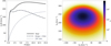Fig. 2

Axisymmetric background. Left panel: Circular velocity curve of the background axisymmetric potential described in Sec. 3.1. Right panel: Number density, ρ_N, of stars in velocity space at the Sun’s position from the equilibrium DF described in Sec. 3.2, for a normalization factor such that the total number in the model at the Sun is the same as found in the data within the 300 pc cylinder around the Sun.

3.2 Axisymmetric equilibrium distribution function

The second step of our procedure consisted of choosing an equilibrium DF for the tracer stellar population within the plane. Since we are confined to the plane, we did not attempt here to be fully self-consistent (see, e.g., Binney & Vasiliev 2023), in order to allow for a simple and tractable form of the DF, namely a simple linear combination of two quasi-isothermal DFs, f (J_R, J_φ) = F_thin + ζF_thick, with ζ = 0.05, which are 2D in action space, and which both have the following form (Binney 2010; Binney & McMillan 2011), $F = η \frac{Ω (J_{φ})}{κ (J_{φ}) {\tilde{σ}}_{R}^{2} (J_{φ})} e x p (- \frac{R_{g} (J_{φ})}{h_{R}}) e x p (- \frac{J_{R} κ (J_{φ})}{{\tilde{σ}}_{R}^{2} (J_{φ})}),$ $F = \eta \frac{\Omega(J_\varphi)}{\kappa(J_\varphi) \tilde{\sigma}^2_R(J_\varphi)} {\rm exp} \left( -\frac{R_\mathrm{g}(J_\varphi)}{h_R} \right) {\rm exp}\left( - \frac{J_R\kappa(J_\varphi)}{\tilde{\sigma}^2_R(J_\varphi)} \right),$ (3)

with, R_g, the guiding radius, and, Ω, κ, the circular and epicyclic frequencies, all three depending on the azimuthal action J_φ, h_R, the disk scale length, η, the normalization factor (in units of inverse length squared) of the tracer population, and finally the radial velocity dispersion, ${\tilde{σ}}_{R}$ $\tilde{\sigma}_R$ , depending on the guiding radius as: ${\tilde{σ}}_{R} (R_{g} (J_{φ})) = {\tilde{σ}}_{R} (R_{0}) e x p (- \frac{R_{g} (J_{ϕ}) - R_{0}}{h_{σ, R}}),$ $\tilde{\sigma}_R(R_\mathrm{g}(J_\varphi)) = \tilde{\sigma}_R(R_0) {\rm exp} \left( - \frac{R_\mathrm{g}(J_\phi) - R_0}{h_{\sigma, R}} \right),$ (4)

where h_σ,R is the kinematic scale-length of the tracer population. For F_thin, we set the scale length to h_R = 2.4 kpc in accordance with the potential, the velocity dispersion at the Sun’s position to ${\tilde{σ}}_{R, t h i n} (R_{0}) = 30$ $\tilde{\sigma}_{R,{\rm thin}}(R_0) = 30$ km s⁻¹, and the kinematic scale length to h_{σ_R} = 10 kpc. For F_thick, the only difference is that we set ${\tilde{σ}}_{R, t h i c k} (R_{0}) = 55$ $\tilde{\sigma}_{R,{\rm thick}}(R_0) = 55$ km s⁻¹. Our DF corresponds to a projected 4D DF in phase-space, namely in units of inverse length-squared times inverse velocity-squared, hence corresponding to the 6D DF of the modeled disk populations integrated over heights and vertical velocities. The local velocity distribution at R = R₀ corresponding to this axisymmetric DF is displayed in the right panel of Fig. 2. In practice, the normalization factor was adjusted such that the number of stars in the model at the Sun is the same as found in the data within the cylinder of 300 pc radius and ±300 pc height around the Sun.

Table 2

Parameters of the planar fiducial non-axisymmetric potential fit in Sect. 4.2.

3.3 Non-axisymmetric potential

The third step of our procedure was to add non-axisymmetric modes on top of the axisymmetric background potential Φ₀. The total potential was obtained by adding to Φ₀(R) the real part of the following: $Φ_{tot} (R, φ, t) = Φ_{0} (R) + \sum_{m} ϕ_{b, m} (R, t) e x p [i m (φ - φ_{b,0} - Ω_{b} t)] + \sum_{m} ϕ_{s, m} (R, t) e x p [i m (φ - φ_{s, m, 0} - Ω_{s, m} t)],$ $\Phi_\text{tot}(R,\varphi,t)&= \Phi_0(R) +\sum_{m} \phi_{{\rm b},m} (R,t) \, {\rm exp}[{\rm i} \, m(\varphi - \varphi_\text{b,0} -\Omega_\text{b}t)] \nonumber \\ &\quad +\sum_{m} \phi_{{\rm s},m} (R,t) \, {\rm exp}[{\rm i} \, m(\varphi - \varphi_{{\rm s},m,0} -\Omega_{{\rm s},m}t)],$ (5)

where the current phase and the pattern speed of the bar are, respectively, φ_b,0 and Ω_b, and those of the spiral arms mode, m, respectively, φ_s,m,0 (the present-day spiral phase at the solar position) and Ω_s,m. The amplitude of each mode is given by φ_b,m and φ_s,m for the bar and spirals, respectively. The time, t, is such that currently t = 0.

As was outlined above, the amplitude of the modes of the bar potential is fixed to values that fit well the dynamics of the bulge region. Namely, the bar potential is a superposition of three Fourier modes, with the same parametric form as in Thomas et al. (2023), closely resembling the first three even modes of the bar potential derived in Portail et al. (2017). From this same potential, the bar angle phase was fixed to be φ_b,0 = 28°. The amplitude of each bar mode, m, is given by $ϕ_{b, m} (R, t) = G_{b} (t) A_{b, m} (R) Φ_{0} (R),$ $\phi_{{\rm b},m} (R,t)= G_{\rm b}(t) \, A_{{\rm b},m} (R) \, \Phi_0(R),$ (6)

where G_b(t) ≤ 1 is the growth function for the bar, and A_b,m is the relative amplitude of the bar mode given by $A_{b, m} (R) = K_{b, m} (R / R_{b,max})^{a_{m} - 1} (1 - R / R_{b,max})^{b_{m} - 1},$ $A_{{\rm b},m} (R)= K_{{\rm b},m}~(R/R_\text{b,max})^{a_m-1}(1-R/R_\text{b,max})^{b_m-1},$ (7)

with K_b,m a global amplitude factor and R_b,max the radius at which the mode’s amplitude goes to zero. Importantly, we considered that the amplitude has reached a plateau at the present time G_b(t = 0) = 1. The values of K_b,m, a_m, and b_m for each of the bar modes are presented in Table 2. Only the pattern speed of the bar is adjusted to the location of resonant ridges in local velocity space within our procedure (see the next section).

The spiral arms potential that we propose is an adaptation of the analytical model of Cox & Gomez (2002) described in Monari et al. (2016b), whose amplitude is given by $ϕ_{s, m} (R, t) = G_{s, m} (t) A_{s, m} (R) e x p [i m \frac{l n (R / R_{0})}{t a n p_{s, m}}] Φ_{0} (R),$ $\phi_{{\rm s},m} (R,t)= G_{\rm s, m}(t) \, A_{{\rm s},m} (R) \, {\rm exp}\left[{\rm i} \, m \frac{{\rm ln}(R/R_0)}{{\rm tan} p_{\mathrm{s},m}}\right] \, \Phi_0(R),$ (8)

where G_s,m(t) is the growth function for the spiral arms mode, m, set to G_s,m(t = 0) = 1, p_s,m is the pitch angle, and A_s,m is given by $A_{s, m} (R) = ξ_{s, m} (R) H_{m} (R) \frac{Φ_{0} (R_{0})}{Φ_{0} (R)},$ $A_{{\rm s},m} (R)= \xi_{{\rm s},m}(R) \, H_{m}(R) \, \frac{\Phi_0(R_0)}{\Phi_0(R)},$ (9)

where ξ_s,m is the amplitude factor of the mode, normalized to its value K_s,m at R = R₀ with a radial dependence as follows: $ξ_{s, m} (R) = K_{s, m} \frac{R_{0}^{2} \sin^{2} p_{s, m} + m h_{s, m} R_{0} \sin p_{s, m} + 0.3 m^{2} h_{s, m}^{2}}{R^{2} \sin^{2} p_{s, m} + m h_{s, m} R \sin p_{s, m} + 0.3 m^{2} h_{s, m}^{2}} \times \frac{R^{3} \sin p_{s, m} + 0.3 m h_{s, m} R^{2}}{R_{0}^{3} \sin p_{s, m} + 0.3 m h_{s, m} R_{0}^{2}} .$ $\xi_{{\rm s},m}(R) = K_{{\rm s},m} \frac{R_0^2 \sin^2 p_{s,m} + m h_{\mathrm{s},m} R_0 \sin p_{s,m} + 0.3 m^2 h_{\mathrm{s},m}^2}{ R^2 \sin^2 p_{s,m} + m h_{\mathrm{s},m} R \sin p_{s,m} + 0.3 m^2 h_{\mathrm{s},m}^2}\\ \times \frac{R^3 \sin p_{s,m} + 0.3 m h_{\mathrm{s},m} R^2}{R_0^3 \sin p_{s,m} + 0.3 m h_{\mathrm{s},m} R_0^2}.$ (10)

This adaptation of the Cox & Gomez (2002) potential has the advantage of being easily generalizable to 3D. Here, h_s,m, corresponds to the scale-height of the spiral potential, which we fixed to 130 pc. We have checked that our results are not very sensitive to this parameter and are similar for any values between 100 pc and 300 pc. Finally, H_m, is a radial cutoff function, parametrized by an inner and an outer cutoff, respectively, R_s,m,min and R_s,m,max. The function is simply²: $H_{m} (R) = {\begin{cases} 1 if R_{s, m, m i n} \leq R \leq R_{s, m, m a x}, \\ 0 otherwise . \end{cases}$ $H_{m}(R) = \begin{cases} 1 & \text{if } R_{{\rm s},m,{\rm min}} \leq R \leq R_{{\rm s},m,{\rm max}}, \\ 0 & \text{otherwise}. \end{cases}$ (11)

These cutoffs are determined from the pattern speeds of the bar and spiral modes in the next section. The parameters of the spiral arms (for each mode: amplitude, K_s,m, pitch angle, p_s,m, presentday phase at the solar position, φ_sm,0, and pattern speed, Ω_s,m) adjusted to the data in the next section, together with the bar pattern speed, Ω_b.

4 Fitting procedure and results

4.1 Bar-only model

With all the parametric components of the potential defined above, we were then in a position to launch our backward integrations to adjust the parameters to the data. As is outlined above, the amplitude of the modes and the phase of the bar potential are fixed to values that fit well the dynamics of the bulge region. Only the pattern speed of the bar was then adjusted to the location of resonant ridges in local velocity space, excluding the spiral arms from the model.

Another hyperparameter to adjust and then fix is the (dummy) integration time, T_int, within the backward integration context. This will not affect the location of ridges in local velocity space, but will affect their apparent “sharpness”. As in Dehnen (2000), we separated the total integration time into two equal-time phases of growth of the bar and plateau of its amplitude, with the following growth function: $G_{b} (t) = {\begin{cases} 1 if - \frac{T_{i n t}}{2} \leq t \leq 0, \\ \frac{3}{16} T^{5} - \frac{5}{8} T^{3} + \frac{15}{16} T + \frac{1}{2} if - T_{i n t} < t < - \frac{T_{i n t}}{2}, \end{cases}$ $G_\mathrm{b}(t) = \begin{cases} 1 & \text{if } -\frac{T_{\rm int}}{2} \leq t \leq 0, \\ \frac{3}{16}{\cal T}^5 - \frac{5}{8}{\cal T}^3 + \frac{15}{16}{\cal T} + \frac{1}{2} & \text{if } -T_{\rm int} < t < -\frac{T_{\rm int}}{2}, \end{cases}$ (12)

where $T \equiv (4 t + 3 T_{i n t}) / T_{i n t}$ ${\cal T} \equiv (4t+3T_{\rm int})/T_{\rm int}$ . We chose to adjust those two parameters (pattern speed and dummy integration time) to the 1D distribution of stars in the solar neighborhood for azimuthal velocities within 90 kms⁻¹ < V_φ < 330 kms⁻¹ at V_R = 100 kms⁻¹. This distribution is shown in Fig. 3. The choice of analyzing the ridges at high V_R prevents them from being “contaminated” by the additional effect of spiral arms since, as we shall see in the next subsection, these distort local velocity space mostly in the central regions of the velocity ellipsoid. This adjustment of the bar pattern speed was made in the solar neighborhood, which is the most complete volume, so that peaks and valleys are not missing.

Quantitatively, we compared the sum of the squares of the differences of the 1D distribution of azimuthal velocities in each bin of 2 km s⁻¹ between the Gaia RVS disk sample and the bar-only model. Only the location of the peaks matters here, so the DF renormalization was applied only in the small V_R range considered in Fig. 3, instead of the DF normalization applied within the whole local velocity space in all other instances. We find the best match at Ω_b = 37 km s⁻¹ kpc⁻¹ for a total (dummy) integration time of 543 Myr, corresponding to 3.2 rotations of the bar. Note, however, that the velocity peak that can be attributed to Bobylev moving group, or lower part of the Hercules bimodality (at V_φ ~ 160 km s⁻¹ in Fig. 3), is not recovered, and is never so by a bar-only model that also reproduces the hat at large V_φ. Our best value of the pattern speed places the corotation radius of the bar at R = 6.6 kpc and its OLR radius at R = 11 kpc.

In the first column of Fig. 4, we display the distribution of (V_R , V_φ) velocities at the solar position (setting the value to zero in pixels with no stars in the data within 300 pc from the Sun), of the local (J_φ, J_R) action distribution, as well as the median Galactocentric radial velocity V_R as a function of position within the Galactic plane. Remarkably, the local kinematic distribution corresponding to this bar-only model is already very similar to the observed one, without any additional contribution from spiral arms (see also Monari et al. 2019b, for a less quantitative but similar conclusion). The success of this bar model at producing so many features resembling the observed local kinematic distribution comes from the signatures of the Lindblad resonances of its multiple modes. We confirm this in the Appendix, where we provide a simple formula based on constant energy lines within the improved epicyclic formalism of Dehnen (1999a) in order to evaluate the approximate location of the signature of each bar resonance in local velocity space. At V_R = 100 km s⁻¹, these approximate locations of the bar resonances are also indicated as small dashes on top of Fig. 3. However, as it also appears clearly in the third row of Fig. 4, the bar-only model produces a dipolar structure of median radial velocities within the plane, far from the observed one. This implies that other dynamical ingredients are required to reproduce this median velocity field, which is the topic of the following subsection. Another clear defect of the bar-only model, locally, is that the Sirius moving group does not stand out in local velocity space. Quantitatively, if one considers the density of stars within a strip of V_φ between 250 km s⁻¹ and 260 km s⁻¹ in local velocity space, and compares the value at V_R = −12 km s⁻¹ to that at V_R = 0 km s⁻¹, one gets an increase of ~25% in the data at V_R = −12 km s⁻¹ (the Sirius peak), while one gets a decrease of 11% in the bar-only model (almost identical to the axisymmetric case). This indicates that Sirius is likely caused by spiral arms.

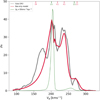Fig. 3

1D distribution of the azimuthal velocity of stars in the solar neighborhood within 99 km s⁻¹ < V_R < 101 kms⁻¹, a region of velocity space where the bar impact dominates the distribution (over potential spiral arms signatures). In gray is the stellar distribution from the Gaia RVS disk sample in the solar neighborhood, smoothed with the Savitzky-Golay filter from the SciPy library. Red line: Renormalized best bar-only model at V_R = 100 km s⁻¹, with pattern speed Ω_b = 37 kms⁻¹kpc⁻¹. For reference, we are providing the results for Ω_b = 55 km s⁻¹ kpc⁻¹ (green line), where only the 1:1 resonance leaves a small signature at higher V_φ than the strong OLR peak. The approximate locations of the different resonances evaluated from Eq. (A.5) are represented as red (Ω_b = 37 km s⁻¹ kpc⁻¹) and green (Ω_b = 55 km s⁻¹ kpc⁻¹) dashes on top of the plot.

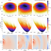Fig. 4

From left to right, the columns correspond to the bar-only model, the Gaia RVS disk sample, and our fiducial non-axisymmetric model, respectively. Top row: 2D histogram of stars in the local (V_R, V_φ) plane defined on [−200,200] kms⁻¹ × [0,400] kms⁻¹, binned with bins of size (1 kms⁻¹)². Middle row: 2D histogram of the number density of stars in the (J_R, Jφ) plane defined on [0,400] kms⁻¹ kpc⁻¹ × [800,2600] km s⁻¹ kpc⁻¹, binned with bins of size (3 × 2 km² s⁻² kpc⁻²). For this, the velocities (V_R, V_φ) have been transformed to actions (J_R, J_φ) with AGAMA. Bottom row: Median ${\tilde{V}}_{R} (x, y)$ $\tilde{V}_{R}$ $(x,y)$ shown in the (x, y) plane defined on [4,12] kpc × [−4,4] kpc, and binned with bins of size (250 pc)² for the data and (50 pc)² for the models. The cross locates the Sun and circles (with sizes proportional to the weights, the lowest weights being dots) in the middle panel (data) indicate the selected points where the fit has been performed. All panels were smoothed with a bilinear interpolation.

4.2 Adding spiral arms

Given the failure of the bar-only model to reproduce the median radial velocity field, the next step taken was to add non-axisymmetric modes corresponding to spiral arms. We started by adding a single mode on top of the bar-only model (i.e., with fixed Ω_b = 37 kms⁻¹ kpc⁻¹), with multiplicity m ∈ [1,2,3,4]. We fixed the scale height to be the same as that of the gas component of the background potential, h_s,m = 130 pc, the outer cutoff to be the OLR of the spiral, and the inner cutoff to be the larger between the corotation radius of the bar and the ILR of the spiral (so that the spiral lives between its ILR and OLR but does not penetrate within the corotation of the bar). The growth function G_s,m(t) has the same form as the bar, and we fixed the integration time to exactly one full rotation of the spiral arm mode. In many other attempts, even allowing more than one rotation and a different growth time, the best candidates in the method that follows tend to converge close to the preferred values we found.

The exploration of the whole parameter space with the backward integration method over a large portion of phase-space is computationally very costly, which led us to select the following strategy to fit the Galaxy model to the Gaia data. The fit was realized with the differential evolution method of Storn & Price (1997), a global genetic optimization method implemented in the Python SciPy library. This algorithm minimizes an objective function, set to be a weighted error function $L = \sum_{i} ({\tilde{V}}_{R, i}^{m o d e l} - {\tilde{V}}_{R, i}^{d a t a})^{2} / σ_{i}^{2}$ ${\cal L} = \sum_i (\tilde{V}^{\rm model}_{R,i}-\tilde{V}^{\rm data}_{R,i})^2/\sigma_i^2$ , comparing median radial velocities from model and data on a small selection of points (x_i, y_i) with weights 1/σ_i. The observed median radial velocities ${\tilde{V}}_{R, i}^{d a t a}$ $\tilde{V}^{\rm data}_{R,i}$ were calculated within bins of size 250 pc around the selected point (x_i, y_i), while the model median radial velocities are the computed median of the V_R distribution at the selected point, i.e. the model DF values in the (V_R, V_φ) plane integrated over V_φ. The choice of the selected points and their respective weights was a delicate one. The number of points must be limited in order to limit the computation time, but this also means that they must be chosen at ‘strategic’ positions and not simply on a uniform grid. Moreover, simply weighting them by the number of stars in the data would give too much weight to the solar vicinity over the entire area of the fit. The first point to which we nevertheless still gave the highest weight, 1/σ₀, is the solar position (x₀, y₀). We then needed to choose points that are representative of the variations of the (positive and negative) values of the median radial velocity all over the plane. Adding spiral arms invariably runs the risk of not preserving the roughly correct radial velocity gradient from the bar in the region around (x₁, y₁) = (7.0 kpc, 3.5 kpc) and (x₂, y₂) = (7.0 kpc, 1.0 kpc), but it is needed to change the sign of V_R at (x₃, y₃) = (9.0 kpc, 0.0 kpc). These were our three second-most important points, all with σi= 2σ₀. We then chose two pairs of points along constant y axes that encapsulate the positive-negative variations in the median radial velocity field, (x₄, y₄) = (6.5 kpc, 0.0 kpc), (x₅, y₅) = (10.0 kpc, 0.0 kpc), (x₆, y₆) = (7.0 kpc, −3.0 kpc), and (x₇, y₇) = (10.0 kpc, −.0 kpc), with σi = 3σ₀. In order to capture the clear spiral feature at the bottom left of the plane, we also added two points, (x₈, y₈) = (6.0 kpc, −2.5 kpc) and (x₉, y₉) = (7.5 kpc, −2.5 kpc), with σi = 5σ₀. We finally imposed a constraint in the outer disk, (x₁₀, y₁₀) = (11.5 kpc, 1.0 kpc) and (x₁₁,y₁₁) = (12.0 kpc, 0.0 kpc), also with σi = 5σ₀. These were the essential points of our fit. We added on top of this a set of low-weight points with the sole function of helping to guide the fit, (x₁₂, y₁₂) = (9.0 kpc, −3.0 kpc), (x₁₃, y₁₃) = (9.0 kpc, 3.5 kpc), (x₁₄, y₁₄) = (i0.0 kpc, 3.5 kpc), and (x₁₅,y₁₅) = (12.0 kpc, 3.5 kpc), all with σi = 100σ₀. All the selected points are indicated as circles in the bottom-middle panel of Fig. 4. This selection of points and their weights hereafter plays the role of a prior on what the most important regions of configuration space are.

For our genetic algorithm, let us now define our population of candidate solutions in parameter space as a_i,g, with 1 ≤ i ≤ n and 1 ≤ g ≤ N. This means we consider n candidates for each generation for N generations. In practice, a first generation of candidate solutions is created by picking stochastically many candidate parameters across the parameter space by a Latin hypercube sampling, all while trying to cover most of the parameter space within the bounds specified hereafter. This population is then mutated, candidate by candidate, iteratively, thereby establishing a new generation at each iteration. At each generation g, the mutation of each candidate a_i,g is applied according to the “best1bin” strategy with the following steps:

Select the best parameters candidate (the one minimizing the weighted error function at current generation), a_best,g.
To mutate each candidate a_i,g, randomly select two other parameters vector candidates, a_j,g and a_k,g.
Take a fixed multiplication factor (mutation factor M) of their difference in parameters, M (a_j,g - a_k,g) to get a vector v_i = a_best,g + M (a_j,g - a_k,g).
The new trial vector a_i,g+1 is then built component by component by assigning the value of each parameter either from v_i or from a_i,g according to if a realization of the binomial function between 0 and 1 is smaller or greater than a chosen recombination value C, respectively.
Compute the weighted error function for the trial vector a_i,g+1 : if it performs better in terms of the objective function, it replaces the original candidate in the next generation, otherwise the initial candidate a_i,g remains the same at generation g + 1.
The convergence criteria are met when the standard deviation of the population objective function values at a given generation is smaller than 1% of the mean objective function value of all candidates in the population in that generation. The final a_best,g=N candidate is kept.

We kept the standard values of the algorithm hyperparameters, notably population size n (15 times the number of parameters), the recombination value C = 0.7, and the mutation factor M, a random variable with values between 0.5 and 1. This method was chosen since it is extremely efficient at converging efficiently over a large parameter space. The selection of points and their weights plays the role of a prior in determining the most important regions of configuration space. However, contrary to a classical Bayesian method, no posterior or well-defined error bars can be given. Therefore, we are not in a position to provide error bars, and we cannot exclude that our best candidate models found hereafter may be local minima in parameter space. Further improvements of the present work should address this question, together with taking into account a Gaia selection function (e.g., Castro-Ginard et al. 2023).

We first attempted to fit only one spiral arms mode, allowing pitch angles to vary between 6° and 30°, the phase to vary all over 360°, the potential amplitude to vary from zero up to 0.2%, and the pattern speed from 10 km s⁻¹ kpc⁻¹ up to the pattern speed of the bar: the mode m = 2 performed the best in terms of the objective function among m ∈ [1,2,3,4], with a pattern speed of 13 km s⁻¹ kpc⁻¹. This is the main result of our search, which we shall now seek to refine. Indeed, this preferred single mode model clearly produces a distorted local velocity space, especially a very distorted Sirius-like moving group compared to observations. This is not entirely surprising, as local velocity space has not been used to constrain the fit. We then modified the objective function L with a local constraint, as follows: $L^{'} = L + \sum_{i = 1}^{i = 2} (Δ_{i}^{m o d e l} - Δ_{i}^{d a t a})^{2} / σ_{Δ}^{2}$ ${\cal L}'={\cal L}+\sum_{i=1}^{i=2}(\Delta_i^{\rm model}-\Delta_i^{\rm data})^2/\sigma_\Delta^2$ , where Δ_i is the location of the 1D V_R distribution peak at V_φ = 250 km s⁻¹ (i = 1) and at V_φ = 260 km s⁻¹ (i = 2) at the Sun, and σΔ = 3σ₀ in both cases. Using L′ , however, still leads to a best candidate with a distorted Sirius moving group in local velocity space when considering a single m = 2 mode.

Then, in order to possibly improve over this model, we attempted a new fit that adds a second spiral mode with multiplicity m = 3 or m = 4, together with the first one and the bar. We assumed the m = 2 spiral to have a range of pattern speeds 10 km s⁻¹ kpc⁻¹ < Ω_s,2 < 14 km s⁻¹ kpc⁻¹, close to the value found for the single mode fit, which we aim to improve upon. To reduce the parameter space, the amplitude of the second higher mode - whose pattern speed and pitch angle are allowed to vary from 10 km s⁻¹ kpc⁻¹ up to the pattern speed of the bar and from 6° to 30° respectively - was fixed with the equation proposed by Hamilton (2024), relating the respective amplitude of both modes to their pattern speed and pitch angle, namely as being inversely proportional to the product of their pattern speed squared with the tangent of their pitch angle (hence a higher amplitude for lower pattern speed and lower pitch angle). To further reduce parameter space, we imposed that the sum of the local density contrasts for both spiral modes be smaller than 35%, checking a posteriori that this limit would not be reached by our best candidate. To compute the surface density contrast of each mode, we took the ratio between the integrated surface density at the Sun of the axisymmetric baryonic component and the spiral arms surface density corresponding to the Cox & Gomez (2002) potential (see also Monari et al. 2016b). In our analysis, we found that the secondary m = 3 spiral mode does complement the stronger mode better than the m = 4 one in terms of the objective function. Adding this second m = 3 mode allowed us to taper and regularize the signature of the Sirius moving group in local velocity space while improving slightly the median radial velocity map. To further polish the parameters of this best candidate found with our global optimization method, we then performed a fine search with a gradient descent in a narrow range of parameter space (1 km s⁻¹ kpc⁻¹ wide in pattern speed, 6° wide in phase, 2° wide in pitch angle, and 0.04% wide in potential amplitude, K_s,2) around our best candidate solution, with the Limited-memory Broyden-Fletcher-Goldfarb-Shanno (L-BFGS-B) algorithm implemented in Scipy. The solution thus found constitutes our fiducial model.

The final parameters of this fiducial model are presented in Table 2, while its local velocity and action space distribution, and median radial velocity map, are presented in the third column of Fig. 4. The improvement of the median radial velocity map compared to the bar-only model is striking, but there are also subtle improvements in local velocity space, in particular, a better representation of moving groups close to the center of the velocity ellipsoid. For Sirius, if one reconsiders the density of stars within a strip of V_φ between 250 km s⁻¹ and 260 km s⁻¹, one now gets an increase of5% at V_R = −12 km s⁻¹ compared to V_R = 0 km s⁻¹ in the model. This is still a significantly smaller peak than in the data (~25%), which will require further investigations, but it is a significant improvement upon the decrease of 11% in the bar-only model. In the next section, we qualitatively compare the predictions of this fiducial model to those of other observables.

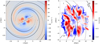Fig. 5

Left panel: Median radial velocity, Ṽ_R, for the fiducial non-axisymmetric model in the disk plane (x,y) defined on [−13,13] kpc × [−13, 13] kpc binned with (250 pc)² bins. Right panel: Adaptation of panel B in figure 1 of Poggio et al. (2021) with over-densities of young upper main sequence stars in red tracing the position of the arms segments. Both panels display the bar position of our fiducial model with dashed black lines, the major m = 2 (black) and minor m = 3 (gray) spiral locations of our fiducial model as continuous and dotted black and gray lines, respectively. The continuous lines indicate the maximum overdensity of the model spirals as a function of radius from their (negative) potential minimum, down to the cutoff radius. The dotted line then traces an arc of a circle at each cutoff radius, until the point where the spiral potential reaches zero. In both panels, the cross represents the Sun’s position. The overdensity maps of young stars following Poggio et al. (2021) were generated from https://github.com/epoggio/Spiral_arms_EDR3.git.

5 Predictions and applications of the model

The fiducial model presented in Table 2 has been adjusted to data with zero prior on the spiral arms’ locations. One can now check how well the model performs in recovering the position of known spiral arms of the Galaxy, as well as how it fares in reproducing other observables, such as the azimuthal velocity field or the detailed locations of moving groups across the disk.

5.1 Locations of spiral arms

In Fig. 5, we present the global radial velocity map predicted by our fiducial model, together with the location of the bar and of the maximum density of the two dynamically-fitted spiral arm modes³. We also compare the location of those arms to the overdensities of young upper main sequence stars identified in Poggio et al. (2021). As it appears clearly in this figure, the strongest m = 2 mode nicely matches the location of the CruxScutum arm close to the Galactic bar (although this arm location is also often labeled as a continuation of the Carina-Sagittarius arm), of the Local arm close to the Sun, and of the Outer arm. However, the distribution of young stars is a consequence of the distribution of the gas, while what we trace is the potential. Therefore, it is most useful to note that our results also appear in line with the findings of Widmark & Naik (2024), who found the Local arm to be a strong local over-density, with a contrast density of roughly 20%, close to the local over-density of 24.9% within our model. Since the pattern speed of the m = 2 spiral is smaller than that of the bar, this could be interpreted as a recent disconnection (52.5 Myr ago) from the bar in the Crux-Scutum region, in accordance with the findings of Vislosky et al. (2024). On the other hand, the weaker m = 3 spiral nicely matches the location of the Carina-Sagittarius and Perseus arms. It is remarkable that a purely dynamical fit mostly recovers the location of known spiral arm over-densities within the disk.

Another interesting quantity to compare our model predictions with is the median J_R as a function of position in the disk. Indeed, Palicio et al. (2023) identified spiral arm structures in the disk from the median J̃_R values as a function of position. We reproduce such a map from the Gaia RVS data within the extended solar neighborhood, in Fig. 6, and overlay the location of the spiral arms from our fiducial model. We also compute the median axisymmetric J̃_R values from our model, starting from the same grid of velocities as before at each location in the plane, then computing the corresponding radial actions with AGAMA (in the axisymmetric background potential), and computing the median from the DF values. Again, the a posteriori qualitative agreement with the data is remarkable. Note that the increase in median axisymmetric J̃_R is positively associated with the presence of spiral arms in our model, in accordance with the findings of Debattista et al. (2025) when considering instantaneous axisymmetric actions. In N-body simulations, one typically needs to average actions over a long-enough timescale to even better track the spirals for low values (Debattista et al. 2025) of the median time-averaged radial action. In our case, the important takeaway is the a posteriori qualitative agreement between the data and model for the instantaneous J̃_R, without having used this quantity in the fitting procedure.

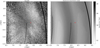Fig. 6

Median J_R as a function of position in the data of the extended solar neighborhood (left panel) and in the model (right panel). The lines indicate the location of spiral arm segments in the model, and the red cross indicates the Sun’s position.

5.2 Azimuthal velocity field

An interesting quantity to look at in principle is the variation in the median azimuthal velocity at a fixed Galactocentric radius, as this is also a clear signature of the non-axisymmetry of the potential. To avoid being dominated by the background DF and axisymmetric potential, one can plot from the data the value $Δ {\tilde{V}}_{φ} \equiv {\tilde{V}}_{φ} (x, y) - {\tilde{V}}_{φ} (R)$ $\Delta \tilde{V}_{\varphi} \equiv \tilde{V}_{\varphi}(x,y) - \tilde{V}_{\varphi}(R)$ , in the (x, y) plane. This is shown in the left panel of Fig. 7. One drawback of showing this quantity is that the azimuthal concatenation at fixed R can only be done in the region where data are available, which is why it was not obvious how to implement such a quantity as a target for the fit itself. From our fiducial model, on the other hand, one can directly subtract from the median radial velocity at each position the median radial velocity obtained from the background DF at the same location. Similar trends to the data can be seen in the model, although the two quantities are not straightforward to compare quantitatively.

5.3 Median radial velocity in the azimuth-angular momentum plane

An interesting projection of Gaia data (see, e.g., Friske & Schönrich 2019; Monari et al. 2019a; Trick et al. 2021; Chiba et al. 2021) is the structure of median (or mean) radial velocity in the azimuth-angular momentum plane. In Fig. 8, we display the median radial velocity in the (J_φ, φ) plane for stars within a box [1300, 3000] km s⁻¹ kpc × [−0.67, 0.67] rad, within 5 kpc < x < 12 kpc and within −4 kpc < y < 4 kpc. To compute the median values in the model, we first fix an azimuth φ_i every 0.01 rad, then consider radii R_j spaced 10 pc from one another. Next, for each point we compute the DF with the backward integration method for different velocities V_R and $V_{φ, n} = \frac{J_{φ, n}}{R_{j}}$ $V_{\varphi,n} = \frac{J_{\varphi,n}}{R_{j}}$ . We then fix J_φ,n and sum the values of the DF for all radii R_j, and we compute the median radial velocity for each (φi, J_ψ,n). The qualitative agreement with the data is acceptable, although one can note that the signatures become weak at low J_ψ in the model. This can be related to the fact that our non-self-consistent procedure is not particularly reliable in the very inner disk close to the bar region. It could also reveal that our constant pattern speed bar is not enough to explain the richness of the data within this plane (Chiba et al. 2021), and that we are missing the effect of vertical perturbations (e.g., Laporte et al. 2019, 2020), as well as accreted prograde structures, although all this would require further investigations.

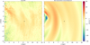Fig. 7

Left panel: Difference of the median azimuthal velocity compared to its average value at fixed R in the Gaia RVS data, $Δ {\tilde{V}}_{φ} \equiv {\tilde{V}}_{φ} (x, y) - {\tilde{V}}_{φ} (R)$ $\Delta \tilde{V}_{\varphi} \equiv \tilde{V}_{\varphi}(x,y) - \tilde{V}_{\varphi}(R)$ , in the (x, y) plane defined on [4,12] kpc × [−4,4] kpc, binned with (125 pc)² bins. Right panel: Difference between the median azimuthal velocity of the fiducial model and that of the background axisymmetric DF. In both panels, the black cross indicates the Sun’s position.

5.4 Moving groups across the disk

In Bernet et al. (2022, 2024), a methodology was developed to perform a blind search for moving groups in Gaia data across the whole disk, based on the execution of a wavelet transform in independent small volumes of the disk followed by a grouping into global structures with the Breadth-first search algorithm from Graph Theory. Fixing a given V_R, one can then, for instance, look at the evolution of the location of moving groups in the (R, V_φ) plane at the azimuth of the Sun, or in the (φ, V_φ) plane at the radius of the Sun. In Fig. 9, we overlay the structures found in Gaia DR3 on top of the density from our model. The azimuthal distribution of moving groups (right panels of Fig. 9) is well in line with the slopes from our model at the solar radius, while the radial distribution at the solar azimuth (left panels of Fig. 9) also appears globally in line with the data apart from the low Vφ ≤ 200 km s⁻¹ region for small R ≤ 6.5kpc (the ridges of the model having a much too high slope in that region of phase-space), where the bar self-gravity is probably having a non-negligible effect on the data.

Interestingly, in the model, the Hercules moving group at the solar radius appears to result from the merging of two ridges at smaller radii, seen as dark regions in Fig. 9 in the underlying density of the model, one with a slope compatible with the observed radial gradient of the Hercules moving group, essentially caused by the bar, and another one with a larger slope, mostly due to spiral arms. This is especially clear at positive V_R, where the two ridges are clearly separated at R < 7 kpc in the model, while this separation appears to leave a similar signature within the data, too. At V_R = 0, the split can also be seen, although it also merges with the inner continuation of the Hyades moving group. At negative V_R, the agreement is less good, though in the region where Hercules is expected to dominate less: the second ridge of Hercules overlaps with the Hyades ridge at R ~ 7 kpc in the model, while in the data this is only seen as a small upward bend in the Hyades ridge, corresponding to the merging of the ridges in the model. This second Hercules ridge is clearly an effect of spiral arms, while the major Hercules one is produced by the bar alone. The joint effect of the multiple bar modes in the present model, together with the axisymmetric background potential used, might explain the differences with Bernet et al. (2024).

Conversely, we applied the method of Bernet et al. (2022, 2024) on the model and overlay in Fig. 10 the detected groups on top of Gaia data at different radii at the azimuth of the Sun, and at different azimuths at the solar radius. Visually, some features are strikingly similar in the model and data. An interesting point to note is that, even though not clearly visible by eye, the model does seem to recover an overdensity at the Sun’s position (bottom right feature in the second panels from the left in Fig. 10) that can be identified with the location of the Bobylev and Hercules-2 bimodality of Hercules, although much less strongly than in the data.

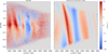Fig. 8

Median radial velocity in the (φ, J_φ) plane defined on [−0.78,0.78]rad × [1000,3000] km s⁻¹ kpc⁻¹, binned with bins of size (0.005 × 2.5 rad × kms⁻¹ kpc⁻¹). Left panel: the Gaia RVS disk sample. Right: the fiducial non-axisymmetric model. Points outside 5 kpc < × < 12 kpc and −4 kpc < y < 4 kpc are excluded in both the data and model.

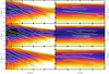Fig. 9

2D histogram distribution of the normalized fiducial model at fixed azimuth φ = 0° (left column), at fixed radius R = R₀ (right column) and at fixed V_R for each row (V_R = 56 km s⁻¹, V_R = 0 km s⁻¹ and V_R = −56 km s⁻¹). The white (and green) lines display the main ridges identified in Gaia DR3 data with the wavelet transform method developed in Bernet et al. (2022, 2024). A thicker green line denotes the Hercules ridge.

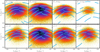Fig. 10

2D histogram distribution of the Gaia RVS disk sample in the (V_R, V_φ) plane for stars within |φ| < 2.4° and |R - R_i| < 300 pc at different radii R_i ∈ [7.3, 8.3, 9.3, 11.3] kpc (top row), and for stars within an annulus |R - R₀| < 300 pc and $| φ - φ_{j} | < \arctan (\frac{300}{8275})$ $|\varphi - \varphi_j| < \arctan\left(\frac{300}{8275}\right)$ at different azimuthal angles φ_j ∈ [−10°, 0°, 5°, 10°] (bottom row). The colored lines show the peaks identified in our model with the method of Bernet et al. (2022, 2024).

5.5 Orbit of the Sun

As an example of application of our model, we propose to compare the in-plane orbit of the Sun in the background axisymmetric model to that in our fiducial non-axisymmetric one. The result is displayed in Fig. 11. It is mostly illustrative, and should not be over-interpreted, given that the vertical motions are neglected. In the axisymmetric case, the radial period is 161.5 Myr, and the Sun is now close to reaching its pericenter. The time between the last pericentric passage and the one that we are about to reach is a bit smaller in the non-axisymmetric model, namely 154.5 Myr. The previous pericentric passage, which happened a bit later in the non-axisymmetric model, was also closer to the Galactic center than in the axisymmetric case. The last apocenter was very similar in both models, but the next-to-last one was further away in the outer Galaxy in the non-axisymmetric case, for which radial amplitudes are typically larger. If we look at the evolution of the surface density at the Sun’s position with time, the picture becomes more complicated. The time between the last surface density maximum and the one that we are about to reach (i.e., still 161.5 Myr in the axisymmetric case) is a bit larger in the non-axisymmetric case, namely 185 Myr, because we shall be temporarily following the Local arm overdensity on our journey back to the outer disk. Also, when looking back at t ~ −250 Myr, the apocenter that corresponds to a minimum in the surface density of the axisymmetric model does actually correspond to a local maximum in the non-axisymmetric case, because the Sun was also following a spiral arm at that time. This could have interesting consequences in studying cyclic sedimentation on Earth on long timescales (e.g., Boulila et al. 2018). Since spiral arms are generally expected to arise from a recurrent cycle of groove or edge modes, it is, however, impossible to trace back the Sun’s orbit on longer timescales than a few 100 Myr, at least without resorting to detailed chemodynamical modeling of the evolution of the whole Galactic disk.

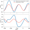Fig. 11

Top panel: Galactocentric radius of the Sun as a function of time in the background axisymmetric (orange) and fiducial non-axisymmetric (blue) models. Bottom panel: Evolution of the surface density at the Sun’s position with time.

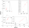Fig. 12

Implications of the non-axisymmetries for the orbits of young associations, illustrated by integrating four young associations for 50 Myr forward in the fiducial potential and then backward in time with both the erroneous axisymmetric model (red) and the fiducial one (black). The insets show zoom-ins around the regions of the associations.

5.6 Orbits of young associations

Young (~50 Myr) stellar associations can typically be traced back to their original position by integrating their orbits backward in a given Galactic potential. To illustrate the importance of taking into account the non-axisymmetries of the potential for such a procedure, we integrate forward in time for 50 Myr four archetypal young stellar associations at different positions in the Galactic disk within our fiducial non-axisymmetric model. Each association is represented by 20 stars that are dispersed in velocity and space with Gaussians of standard deviation of 1 km s⁻¹ in V_R and V_φ around the circular velocity, and of 2 pc around the positions (x, y) = (10.6 kpc, −2.4 kpc), (8.7 kpc, −0.3 kpc), (7.1 kpc, 0.4 kpc), (6.0 kpc, −0.5 kpc). We then integrate them backward in time, both in the fiducial non-axisymmetric model and in the background axisymmetric model. The associations typically go back to a position that can be erroneous by more than 150 pc in the axisymmetric case, with an elongated shape very different from the true original configuration (Fig. 12).

6 Discussion and conclusions

We used the in-plane velocities of a sample of disk stars with 6D phase-space information from Gaia-StarHorse in order to fit a Galactic potential model that includes a detailed parametric shape for the bar and spiral arms, using the backward integration method. The adjusted observable quantities were the median Galactocentric radial velocity, for a selection of points within the Galactic plane, complemented by additional constraints from local velocity space at the Sun’s position. All the parameters of the fiducial non-axisymmetric potential are summarized in Table 2, within the background axisymmetric potential fixed in Table 1. It is remarkable that such a purely dynamical fit recovers many of the known locations of spiral arm over-densities detected from photometry within the disk (Fig. 5). These spiral arms can be interpreted as groove or edge modes such as those found in N-body simulations. In the solar vicinity, we identify the Local arm as a strong gravitational perturbation, in accordance with independent probes of the local non-axisymmetric potential by Widmark & Naik (2024). We also recover the observed map of median radial actions in the extended solar vicinity (Fig. 6), as well as a good qualitative agreement with the detailed variation with radius and azimuth of moving groups identified in Gaia data (Fig. 9). The latter is truly remarkable, since the model was not directly fit to these phase-space features. The only (locally) fit moving group was Sirius, which is entirely absent from the bar-only model: we note that it is nevertheless still characterized by a weaker peak in the fiducial model than in the data. While our best candidate model may well be a local minimum in parameter space, the latter being particularly vast, especially if letting the parameters of the background axisymmetric density and DF vary too, we nevertheless argue that it can, for the time being, be used as a fiducial non-axisymmetric potential for the Galaxy, for instance in order to confidently integrate in-plane orbits. It can be compared to other recent Galactic potentials such as that of Hunter et al. (2024). The code to generate local velocity space distributions as well as radial velocity maps is made public.

This paper represents only a first quantitative step in the direction of establishing a detailed 3D non-axisymmetric potential for the MW. Future improvements on our present investigations will be to explore its 3D consequences, first in forward test-particle integrations (see, e.g., Faure et al. 2014; Monari et al. 2016b), as both the bar (Thomas et al. 2023) and spiral (Cox & Gomez 2002) potentials can readily be generalized to three dimensions. Let us also note that we have made the assumption that the spiral arms cannot live inside the corotation resonance of the bar (R = 6.6 kpc in our fiducial model), an assumption that could potentially be partially lifted: we already checked that it does not much affect our best candidate model. However, a proper fit of these inner regions of the Galactic disk would require us to make the model self-consistent. The absence of self-consistency can become a serious issue in the innermost parts of the Galaxy, where the bar perturbation is itself the tracer. Some deficiencies of our model at low radii and low angular momenta have indeed already been identified in Figs. 8 and 9. Although beyond the scope of the present work, future improvements on our model might rely on an adaptation of the self-consistent made-to-measure method in order to account for self-consistency. One should also point out that the background model (axisymmetric potential and DF) has not been fit here, and could in principle also be adjusted to the data. This would increase the parameter space and might require us to use machine learning methods to efficiently explore the full parameter space. A parallel improvement will be to incorporate a detailed selection function in the fitting procedure (e.g., Castro-Ginard et al. 2023; Khanna et al. 2024), and compute a proper posterior (and error bars) on the best-fit parameters, while perhaps attempting to separate the stellar populations into distinct DFs. Finally, when moving to three dimensions, it is obvious that vertical perturbations of the disk, for example, from the Sagittarius dwarf, will have to be included too, together with a possible time-variation in the bar pattern speed.

In summary, the fiducial model presented here, reproducing a larger amount of observables than ever before, does represent a significant advance in our understanding of the non-axisymmetric structure of the MW disk. However, it is important to recognize its limitations and to continue improving it in order to obtain an even more accurate representation of our Galaxy.

Data availability

The “Spiral and Bar Backward Integration” (SPIBACK) PyTorch-based code to generate local velocity space distributions as well as median radial velocity maps is publicly available at: https://github.com/yrkhalil/SPIBACK

Acknowledgements

We thank the anonymous referee for constructive comments that helped improve the paper. YRK and BF thank Laurent Navoret for his support and advice throughout the project, as well as insightful comments from Leandro Beraldo e Silva, Pedro Alonso Palicio, Eugene Vasiliev, Jean-Baptiste Fouvry, Jorge Peñarrubia, Ronald Drimmel, and Eloisa Poggio. This work was supported by the Interdisciplinary Thematic Institute IRMIA++, as part of the ITI 2021-2028 program of the University of Strasbourg, CNRS and Inserm, was supported by IdEx Unistra (ANR-10-IDEX-0002), and by SFRI-STRAT’US project (ANR-20-SFRI-0012) under the framework of the French Investments for the Future Program. BF, GM, AS, RI acknowledge funding from the ANR grants ANR-20-CE31-0004 (MWDisc), ANR-19-CE31-0017 (SEGAL) and ANR-18-CE31-0006 (GaDaMa). BF, AS and RI acknowledge funding from the European Research Council (ERC) under the European Union’s Horizon 2020 research and innovation programme (grant agreement No. 834148). MB acknowledges funding from the University of Barcelona’s official doctoral program for the development of a R+D+i project under the PREDOCS-UB grant. TA acknowledges the grant RYC2018-025968-I funded by MCIN/AEI/10.13039/501100011033 and by “ESF Investing in your future”, the grants PID2021-125451NA-I00 and CNS2022-135232 funded by MICIU/AEI/10.13039/501100011033 and by “ERDF A way of making Europe”, by the “European Union” and by the “European Union Next Generation EU/PRTR” and the Institute of Cosmos Sciences University of Barcelona (ICCUB, Unidad de Excelencia ’María de Maeztu’) through grant CEX2019-000918-M. This work has made use of data from the European Space Agency (ESA) mission Gaia (https://www.cosmos.esa.int/gaia), processed by the Gaia Data Processing and Analysis Consortium (DPAC, https://www.cosmos.esa.int/web/gaia/dpac/consortium). Funding for the DPAC has been provided by national institutions, in particular the institutions participating in the Gaia Multilateral Agreement. This research has made use of the SIMBAD database and of the VizieR catalogue access tool, operated at CDS, Strasbourg, France.

Appendix A A simple formula for approximately locating bar resonances in velocity space

In order to evaluate analytically the location of the phase-space resonant zones due to a constant pattern speed bar perturbation, one should define those zones in terms of librating versus circulating orbits after canonically transforming to slow and fast action and angle variables (e.g., Monari et al. 2017; Binney 2020). This is a relatively arduous task, and we propose here a less precise but much faster way to roughly estimate the location of resonant ridges in local velocity space, or more accurately, the surfaces of phase-space where the resonant condition is fulfilled. This simple formula will be, by construction, axisymmetric, which means that one cannot use it to model the changes in the morphology of the resonant surfaces with azimuth. The formula relies on locally drawing constant energy lines in the V_R- V_φ plane within the improved epicyclic formalism presented in Dehnen (1999a). For convenience, we reproduce here their equations 28 and 29 for the radial evolution of an orbit: $R (η) = R_{E} {[1 - e c o s (η)]}^{\frac{γ}{2}},$ $R(\eta) &= R_E\left[1-e \, \mathrm{cos}(\eta)\right]^{\frac{\gamma}{2}},\\$ (A.1) $e = \sqrt{1 - {(\frac{J_{φ}}{J_{φ}^{c i r c}})}^{2}},$ $e &= \sqrt{1-\left(\frac{J_{\varphi}}{J_{\varphi}^{\rm circ}}\right)^2},$ (A.2)

where $J_{φ}^{c i r c}$ $J_{\varphi}^{\rm circ}$ and R_E are, respectively, the angular momentum and radius of a circular orbit of the same energy, γ = γ(R_E) = 2Ω(R_E)/κ(R_E) is the ratio of the circular frequency Ω over the radial epicyclic frequency κ as usual, and e is the eccentricity of the orbit. The phase in radius evolving with time t, namely η(t), is the parameter that represents the position along the path of the orbit, and is defined as a function of the eccentricity and the radial epicyclic frequency (see Eq. (28d) of Dehnen 1999a). For simplicity, we consider that η ~ κt, which in turn means that the radial velocity can be calculated as: $V_{R} = \frac{d R}{d η} \frac{d η}{d t} \sim κ \frac{γ}{2} R (η) \frac{e s i n (η)}{1 - e c o s (η)} = V_{c} (R_{E}) \frac{R}{R_{E}} \frac{e s i n (η)}{1 - e c o s (η)} .$ $V_R = \frac{dR}{d\eta}\frac{d\eta}{dt} \sim \kappa \frac{\gamma}{2}R(\eta)\frac{e \, \mathrm{sin}(\eta)}{1-e \, \mathrm{cos}(\eta)} = V_c(R_E)\frac{R}{R_E}\frac{e \, \mathrm{sin}(\eta)}{1-e \, \mathrm{cos}(\eta)}.$ (A.3)

The azimuthal velocity, on the other hand, can be written as a function of R simply by the conservation of angular momentum: V_φ = J_φ/R(η). Using Eq. A.1 and Eq. A.2, one then gets a closed form equation that relates the changes of V_R along the orbit to those of R, V_φ, and the circular velocity curve: $V_{R} = V_{c} (R_{E}) {(\frac{R}{R_{E}})}^{\frac{γ - 2}{γ}} \sqrt{2 {(\frac{R}{R_{E}})}^{\frac{2}{γ}} - {(\frac{R}{R_{E}})}^{\frac{4}{γ}} - {(\frac{R V_{φ}}{J_{φ}^{c i r c}})}^{2}} .$ $V_R = V_c(R_E)\left(\frac{R}{R_E}\right)^{\frac{\gamma-2}{\gamma}}\sqrt{2\left(\frac{R}{R_E}\right)^{\frac{2}{\gamma}}-\left(\frac{R}{R_E}\right)^{\frac{4}{\gamma}}-\left(\frac{R V_\varphi}{J_{\varphi}^{\rm circ}}\right)^2} .$ (A.4)

All that is left is to impose the constraint that stars be on a surface where the resonant condition is met. Under the assumption that frequencies are functions solely of the energy, the resonant condition is preserved as long as stars share the same $J_{φ}^{c i r c}$ $J_{\varphi}^{\rm circ}$ and R_E, and as longs as these are equal to the radius and angular momentum where the circular orbit is l : m resonant. We refer to these as R_res, such that lκ(R_res) + m [Ω(R_res) - Ωb] = 0, and as $J_{φ}^{r e s} \equiv R_{r e s} V_{c} (R_{r e s})$ $J_{\varphi}^{\rm res} \equiv R_{\rm res} V_c(R_{\rm res})$ , respectively. The final equation for the surfaces of the resonant condition is then: $V_{φ}^{r e s} (R, V_{R}) = \frac{J_{φ}^{r e s}}{R} \sqrt{2 {(\frac{R}{R_{r e s}})}^{\frac{2}{γ}} - {(\frac{R}{R_{r e s}})}^{\frac{4}{γ}} [1 + {(\frac{R_{r e s}}{R} \frac{V_{R}}{V_{c} (R_{r e s})})}^{2}]} .$ $V_\varphi^{\rm res}(R,\,V_R) = \frac{J_{\varphi}^{\rm res}}{R}\sqrt{2\left(\frac{R}{R_{\rm res}}\right)^{\frac{2}{\gamma}}-\left(\frac{R}{R_{\rm res}}\right)^{\frac{4}{\gamma}}\left[1+\left(\frac{R_{\rm res}}{R}\frac{V_R}{V_c(R_{\rm res})}\right)^2\right]}.$ (A.5)

where we reordered the terms to express V_φ as a function of the other phase-space variables.

The application of Eq. A.5 to the V_R-V_φ velocity plane produces for each resonance a curve that is almost identical to Eq. 9 from Dehnen (2000), and is equivalent to drawing lines of constant energy at a given configuration space point, because it is written under the assumption that the orbital frequencies are pure functions of the orbital energy. As can be seen in Fig. A.1, in our best bar model, this formula identifies extremely well the peak of the overdensities produced at R = R₀ by the 6 : 1, 4 : 1, and 2 : 1 outer resonances of the bar. For the (l, m) = (0, 2) corotation resonance, the formula fails, probably because the eccentricity becomes too large, and it rather approximately identifies the lower bound of the resonant zone.

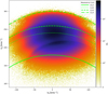Fig. A.1

Resonant lines $V_{φ}^{r e s}$ $V_\varphi^{\rm res}$ as a function of V_R from Eq. A.5 at R = R₀, computed with the potential of Table 1, for a bar pattern speed of 37 km s⁻¹ kpc⁻¹. The lines are overlaid on top of the local velocity space density produced by our preferred bar-only model at the Sun’s position.

References

Al Kazwini, H., Agobert, Q., Siebert, A., et al. 2022, A&A, 658, A50 [NASA ADS] [CrossRef] [EDP Sciences] [Google Scholar]
Amaral, L. H., & Lepine, J. R. D. 1997, MNRAS, 286, 885 [Google Scholar]
Anders, F., Khalatyan, A., Queiroz, A. B. A., et al. 2022, A&A, 658, A91 [NASA ADS] [CrossRef] [EDP Sciences] [Google Scholar]
Antoja, T., Figueras, F., Fernández, D., & Torra, J. 2008, A&A, 490, 135 [NASA ADS] [CrossRef] [EDP Sciences] [Google Scholar]
Antoja, T., Helmi, A., Bienayme, O., et al. 2012, MNRAS, 426, L1 [Google Scholar]
Antoja, T., Helmi, A., Dehnen, W., et al. 2014, A&A, 563, A60 [NASA ADS] [CrossRef] [EDP Sciences] [Google Scholar]
Antoja, T., Helmi, A., Romero-Gómez, M., et al. 2018, Nature, 561, 360 [Google Scholar]
Astropy Collaboration (Price-Whelan, A. M., et al.) 2022, ApJ, 935, 167 [NASA ADS] [CrossRef] [Google Scholar]
Baba, J., Saitoh, T. R., & Wada, K. 2013, ApJ, 763, 46 [Google Scholar]
Benjamin, R. A., Churchwell, E., Babler, B. L., et al. 2005, ApJ, 630, L149 [NASA ADS] [CrossRef] [Google Scholar]
Beraldo e Silva, L., de Siqueira Pedra, W., & Valluri, M. 2019, ApJ, 872, 20 [Google Scholar]
Bernet, M., Ramos, P., Antoja, T., et al. 2022, A&A, 667, A116 [NASA ADS] [CrossRef] [EDP Sciences] [Google Scholar]
Bernet, M., Ramos, P., Antoja, T., Monari, G., & Famaey, B. 2024, A&A, 686, A92 [NASA ADS] [CrossRef] [EDP Sciences] [Google Scholar]
Binney, J. 2010, MNRAS, 401, 2318 [Google Scholar]
Binney, J. 2012, MNRAS, 426, 1324 [Google Scholar]
Binney, J. 2020, MNRAS, 495, 895 [NASA ADS] [CrossRef] [Google Scholar]
Binney, J., & Tremaine, S. 2008, Galactic Dynamics, 2nd edn. (Princeton University Press) [Google Scholar]
Binney, J., & McMillan, P. 2011, MNRAS, 413, 1889 [NASA ADS] [CrossRef] [Google Scholar]
Binney, J., & Schönrich, R. 2018, MNRAS, 481, 1501 [Google Scholar]
Binney, J., & Vasiliev, E. 2023, MNRAS, 520, 1832 [NASA ADS] [CrossRef] [Google Scholar]
Binney, J., Gerhard, O. E., Stark, A. A., Bally, J., & Uchida, K. I. 1991, MNRAS, 252, 210 [Google Scholar]
Binney, J., Gerhard, O., & Spergel, D. 1997, MNRAS, 288, 365 [NASA ADS] [CrossRef] [Google Scholar]
Bissantz, N., Englmaier, P., & Gerhard, O. 2003, MNRAS, 340, 949 [NASA ADS] [CrossRef] [Google Scholar]
Bland-Hawthorn, J., & Gerhard, O. 2016, ARA&A, 54, 529 [Google Scholar]
Blitz, L., & Spergel, D. N. 1991, ApJ, 379, 631 [Google Scholar]
Boulila, S., Laskar, J., Haq, B. U., Galbrun, B., & Hara, N. 2018, Global Planet. Change, 165, 128 [CrossRef] [Google Scholar]
Callingham, T. M., Cautun, M., Deason, A. J., et al. 2019, MNRAS, 484, 5453 [Google Scholar]
Castro-Ginard, A., McMillan, P. J., Luri, X., et al. 2021, A&A, 652, A162 [NASA ADS] [CrossRef] [EDP Sciences] [Google Scholar]
Castro-Ginard, A., Brown, A. G. A., Kostrzewa-Rutkowska, Z., et al. 2023, A&A, 677, A37 [NASA ADS] [CrossRef] [EDP Sciences] [Google Scholar]
Chen, R. T. Q. 2018, https://github.com/rtqichen/torchdiffeq [Google Scholar]
Chiba, R., & Schönrich, R. 2021, MNRAS, 505, 2412 [NASA ADS] [CrossRef] [Google Scholar]
Chiba, R., Friske, J. K. S., & Schönrich, R. 2021, MNRAS, 500, 4710 [Google Scholar]
Churchwell, E., Babler, B. L., Meade, M. R., et al. 2009, PASP, 121, 213 [Google Scholar]
Clarke, J. P., Wegg, C., Gerhard, O., et al. 2019, MNRAS, 489, 3519 [Google Scholar]
Cox, D. P., & Gomez, G. C. 2002, ApJSS, 142, 261 [Google Scholar]
De Rijcke, S., & Voulis, I. 2016, MNRAS, 456, 2024 [Google Scholar]
De Rijcke, S., Fouvry, J.-B., & Pichon, C. 2019, MNRAS, 484, 3198 [Google Scholar]
de Salas, P. F., & Widmark, A. 2021, Rep. Prog. Phys., 84, 104901 [Google Scholar]
de Vaucouleurs, G. 1964, in The Galaxy and the Magellanic Clouds, 20, ed. F. J. Kerr, 195 [Google Scholar]
Debattista, V. P., Gerhard, O., & Sevenster, M. N. 2002, MNRAS, 334, 355 [Google Scholar]
Debattista, V. P., Khachaturyants, T., Amarante, J. A. S., et al. 2025, MNRAS, 537, 1620 [Google Scholar]
Dehnen, W. 1998, AJ, 115, 2384 [NASA ADS] [CrossRef] [Google Scholar]
Dehnen, W. 1999a, AJ, 118, 1190 [Google Scholar]
Dehnen, W. 1999b, ApJ, 524, L35 [CrossRef] [Google Scholar]
Dehnen, W. 2000, AJ, 119, 800 [NASA ADS] [CrossRef] [Google Scholar]
Dillamore, A. M., Belokurov, V., & Evans, N. W. 2024, MNRAS, 532, 4389 [NASA ADS] [CrossRef] [Google Scholar]
D’Onghia, E., & Aguerri, J. A. L. 2020, ApJ, 890, 117 [CrossRef] [Google Scholar]
Drimmel, R. 2000, A&A, 358, L13 [NASA ADS] [Google Scholar]
Drimmel, R., & Spergel, D. N. 2001, ApJ, 556, 181 [Google Scholar]
Drimmel, R., Khanna, S., Poggio, E., & Skowron, D. M. 2025, A&A, 698, A230 [NASA ADS] [CrossRef] [EDP Sciences] [Google Scholar]
Eilers, A.-C., Hogg, D. W., Rix, H.-W., et al. 2020, ApJ, 900, 186 [Google Scholar]
Englmaier, P., & Gerhard, O. 1999, MNRAS, 304, 512 [NASA ADS] [CrossRef] [Google Scholar]
Famaey, B., & Dejonghe, H. 2003, MNRAS, 340, 752 [NASA ADS] [CrossRef] [Google Scholar]
Famaey, B., Jorissen, A., Luri, X., et al. 2005, A&A, 430, 165 [CrossRef] [EDP Sciences] [Google Scholar]
Famaey, B., Pont, F., Luri, X., et al. 2007, A&A, 461, 957 [NASA ADS] [CrossRef] [EDP Sciences] [Google Scholar]
Famaey, B., Siebert, A., & Jorissen, A. 2008, A&A, 483, 453 [NASA ADS] [CrossRef] [EDP Sciences] [Google Scholar]
Faure, C., Siebert, A., & Famaey, B. 2014, MNRAS, 440, 2564 [CrossRef] [Google Scholar]
Fiteni, K., De Rijcke, S., Debattista, V. P., & Caruana, J. 2024, MNRAS, 529, 4879 [Google Scholar]
Fragkoudi, F., Katz, D., Trick, W., et al. 2019, MNRAS, 488, 3324 [NASA ADS] [Google Scholar]
Frankel, N., Hogg, D. W., Tremaine, S., Price-Whelan, A., & Shen, J. 2024, arXiv e-prints, [arXiv:2407.07149] [Google Scholar]
Friske, J. K. S., & Schönrich, R. 2019, MNRAS, 490, 5414 [Google Scholar]
Fux, R. 1999, A&A, 345, 787 [NASA ADS] [Google Scholar]
Fux, R. 2001, A&A, 373, 511 [NASA ADS] [CrossRef] [EDP Sciences] [Google Scholar]
Gaia Collaboration (Brown, A. G. A., et al.) 2018a, A&A, 616, A1 [NASA ADS] [CrossRef] [EDP Sciences] [Google Scholar]
Gaia Collaboration (Katz, D., et al.) 2018b, A&A, 616, A11 [NASA ADS] [CrossRef] [EDP Sciences] [Google Scholar]
Gaia Collaboration (Brown, A. G. A., et al.) 2021, A&A, 649, A1 [NASA ADS] [CrossRef] [EDP Sciences] [Google Scholar]
Gaia Collaboration (Vallenari, A., et al.) 2023a, A&A, 674, A1 [NASA ADS] [CrossRef] [EDP Sciences] [Google Scholar]
Gaia Collaboration (Drimmel, R., et al.) 2023b, A&A, 674, A37 [CrossRef] [EDP Sciences] [Google Scholar]
Georgelin, Y. M., & Georgelin, Y. P. 1976, A&A, 49, 57 [NASA ADS] [Google Scholar]
Gerhard, O. E., & Vietri, M. 1986, MNRAS, 223, 377 [NASA ADS] [Google Scholar]
Hamilton, C. 2024, MNRAS, 528, 5286 [Google Scholar]
Hamilton, C., Tolman, E. A., Arzamasskiy, L., & Duarte, V. N. 2023, ApJ, 954, 12 [Google Scholar]
Haywood, M., Khoperskov, S., Cerqui, V., et al. 2024, A&A, 690, A147 [NASA ADS] [CrossRef] [EDP Sciences] [Google Scholar]
Hilmi, T., Minchev, I., Buck, T., et al. 2020, MNRAS, 497, 933 [Google Scholar]
Horta Darrington, D., Petersen, M. S., & Peñarrubia, J. 2025, MNRAS, 538, 998 [Google Scholar]
Hunt, J. A. S., & Bovy, J. 2018, MNRAS, 477, 3945 [NASA ADS] [CrossRef] [Google Scholar]
Hunt, J. A. S., & Vasiliev, E. 2025, New A Rev., 100, 101721 [Google Scholar]
Hou, L. G., Han, J. L., & Shi, W. B. 2009, A&A, 499, 473 [NASA ADS] [CrossRef] [EDP Sciences] [Google Scholar]
Hunt, J. A. S., Hong, J., Bovy, J., Kawata, D., & Grand, R. J. J. 2018, MNRAS, 481, 3794 [NASA ADS] [CrossRef] [Google Scholar]
Hunt, J. A. S., Bub, M. W., Bovy, J., et al. 2019, MNRAS, 490, 1026 [NASA ADS] [CrossRef] [Google Scholar]
Hunter, G. H., Sormani, M. C., Beckmann, J. P., et al. 2024, A&A, 692, A216 [NASA ADS] [CrossRef] [EDP Sciences] [Google Scholar]
Ibata, R., Malhan, K., Tenachi, W., et al. 2024, ApJ, 967, 89 [NASA ADS] [CrossRef] [Google Scholar]
Jiao, Y., Hammer, F., Wang, H., et al. 2023, A&A, 678, A208 [NASA ADS] [CrossRef] [EDP Sciences] [Google Scholar]
Khanna, S., Yu, J., Drimmel, R., et al. 2024, arXiv e-prints, [arXiv:2410.22036] [Google Scholar]
Khoperskov, S., & Gerhard, O. 2022, A&A, 663, A38 [NASA ADS] [CrossRef] [EDP Sciences] [Google Scholar]
Khoperskov, S., Gerhard, O., Di Matteo, P., et al. 2020, A&A, 634, L8 [NASA ADS] [CrossRef] [EDP Sciences] [Google Scholar]
Khoperskov, S., Steinmetz, M., Haywood, M., et al. 2024, arXiv e-prints, [arXiv:2411.16866] [Google Scholar]
Laporte, C. F. P., Minchev, I., Johnston, K. V., & Gómez, F. A. 2019, MNRAS, 485, 3134 [Google Scholar]
Laporte, C. F. P., Famaey, B., Monari, G., et al. 2020, A&A, 643, L3 [EDP Sciences] [Google Scholar]
Levine, E. S., Blitz, L., & Heiles, C. 2006, Science, 312, 1773 [NASA ADS] [CrossRef] [Google Scholar]
Li, C., Siebert, A., Monari, G., Famaey, B., & Rozier, S. 2023, MNRAS, 524, 6331 [NASA ADS] [CrossRef] [Google Scholar]
Li, C., Yuan, Z., Monari, G., et al. 2024, A&A, 690, A26 [NASA ADS] [CrossRef] [EDP Sciences] [Google Scholar]
Li, Z., Gerhard, O., Shen, J., Portail, M., & Wegg, C. 2016, ApJ, 824, 13 [NASA ADS] [CrossRef] [Google Scholar]
Lin, C. C., & Shu, F. H. 1964, ApJ, 140, 646 [Google Scholar]
Lin, C. C., Yuan, C., & Shu, F. H. 1969, ApJ, 155, 721 [NASA ADS] [CrossRef] [Google Scholar]
Lucchini, S., D’Onghia, E., & Aguerri, J. A. L. 2024, MNRAS, 531, L14 [CrossRef] [Google Scholar]
Lynden-Bell, D., & Kalnajs, A. J. 1972, MNRAS, 157, 1 [Google Scholar]
Malhan, K., & Ibata, R. A. 2019, MNRAS, 486, 2995 [NASA ADS] [CrossRef] [Google Scholar]
Minchev, I., Nordhaus, J., & Quillen, A. C. 2007, ApJ, 664, L31 [NASA ADS] [CrossRef] [Google Scholar]
Monari, G., Helmi, A., Antoja, T., & Steinmetz, M. 2014, A&A, 569, A69 [NASA ADS] [CrossRef] [EDP Sciences] [Google Scholar]
Monari, G., Famaey, B., & Siebert, A. 2016a, MNRAS, 457, 2569 [Google Scholar]
Monari, G., Famaey, B., Siebert, A., et al. 2016b, MNRAS, 461, 3835 [Google Scholar]
Monari, G., Famaey, B., Fouvry, J.-B., & Binney, J. 2017, MNRAS, 471, 4314 [NASA ADS] [CrossRef] [Google Scholar]
Monari, G., Famaey, B., Carrillo, I., et al. 2018, A&A, 616, L9 [NASA ADS] [CrossRef] [EDP Sciences] [Google Scholar]
Monari, G., Famaey, B., Siebert, A., et al. 2019a, A&A, 632, A107 [NASA ADS] [CrossRef] [EDP Sciences] [Google Scholar]
Monari, G., Famaey, B., Siebert, A., Wegg, C., & Gerhard, O. 2019b, A&A, 626, A41 [NASA ADS] [CrossRef] [EDP Sciences] [Google Scholar]
Morgan, W. W., Sharpless, S., & Osterbrock, D. 1952, AJ, 57, 3 [Google Scholar]
Oort, J. H., Kerr, F. J., & Westerhout, G. 1958, MNRAS, 118, 379 [NASA ADS] [CrossRef] [Google Scholar]
Ou, X., Eilers, A.-C., Necib, L., & Frebel, A. 2024, MNRAS, 528, 693 [NASA ADS] [CrossRef] [Google Scholar]
Palicio, P. A., Recio-Blanco, A., Poggio, E., et al. 2023, A&A, 670, L7 [NASA ADS] [CrossRef] [EDP Sciences] [Google Scholar]
Paszke, A., Gross, S., Massa, F., et al. 2019, in Advances in Neural Information Processing Systems, 32 (Curran Associates, Inc.), 8024 [Google Scholar]
Pérez-Villegas, A., Portail, M., Wegg, C., & Gerhard, O. 2017, ApJ, 840, L2 [Google Scholar]
Peters, W. L. I. 1975, ApJ, 195, 617 [Google Scholar]
Poggio, E., Drimmel, R., Cantat-Gaudin, T., et al. 2021, A&A, 651, A104 [NASA ADS] [CrossRef] [EDP Sciences] [Google Scholar]
Pompéia, L., Masseron, T., Famaey, B., et al. 2011, MNRAS, 415, 1138 [Google Scholar]
Portail, M., Gerhard, O., Wegg, C., & Ness, M. 2017, MNRAS, 465, 1621 [NASA ADS] [CrossRef] [Google Scholar]
Quillen, A. C., Dougherty, J., Bagley, M. B., Minchev, I., & Comparetta, J. 2011, MNRAS, 417, 762 [NASA ADS] [CrossRef] [Google Scholar]
Ramos, P., Antoja, T., & Figueras, F. 2018, A&A, 619, A72 [NASA ADS] [CrossRef] [EDP Sciences] [Google Scholar]
Reid, M. J., Menten, K. M., Brunthaler, A., et al. 2019, ApJ, 885, 131 [Google Scholar]
Roche, C., Necib, L., Lin, T., Ou, X., & Nguyen, T. 2024, ApJ, 972, 70 [NASA ADS] [CrossRef] [Google Scholar]
Sanders, J. L., & Binney, J. 2016, MNRAS, 457, 2107 [Google Scholar]
Sanders, J. L., Smith, L., & Evans, N. W. 2019, MNRAS, 488, 4552 [NASA ADS] [CrossRef] [Google Scholar]
Sellwood, J. A. 1993, in American Institute of Physics Conference Series, 278, Back to the Galaxy, eds. S. S. Holt & F. Verter, 133 [Google Scholar]
Sellwood, J. A. 2010, MNRAS, 409, 145 [NASA ADS] [CrossRef] [Google Scholar]
Sellwood, J. A., & Carlberg, R. G. 2014, ApJ, 785, 137 [CrossRef] [Google Scholar]
Sellwood, J. A., & Carlberg, R. G. 2019, MNRAS, 489, 116 [CrossRef] [Google Scholar]
Sellwood, J. A., & Masters, K. L. 2022, ARA&A, 60, 73 [NASA ADS] [CrossRef] [Google Scholar]
Shen, J., & Zheng, X.-W. 2020, Res. Astron. Astrophys., 20, 159 [CrossRef] [Google Scholar]
Siebert, A., Famaey, B., Binney, J., et al. 2012, MNRAS, 425, 2335 [Google Scholar]
Sormani, M. C., Binney, J., & Magorrian, J. 2015, MNRAS, 454, 1818 [NASA ADS] [CrossRef] [Google Scholar]
Storn, R., & Price, K. 1997, J. Global Optim., 11, 341 [Google Scholar]
Syer, D., & Tremaine, S. 1996, MNRAS, 282, 223 [Google Scholar]
Thomas, G. F., Famaey, B., Monari, G., et al. 2023, A&A, 678, A180 [NASA ADS] [CrossRef] [EDP Sciences] [Google Scholar]
Tremaine, S., & Weinberg, M. D. 1984, ApJ, 282, L5 [Google Scholar]
Tremaine, S., Frankel, N., & Bovy, J. 2023, MNRAS, 521, 114 [NASA ADS] [CrossRef] [Google Scholar]
Trick, W. H. 2022, MNRAS, 509, 844 [Google Scholar]
Trick, W. H., Coronado, J., & Rix, H.-W. 2019, MNRAS, 484, 3291 [NASA ADS] [CrossRef] [Google Scholar]
Trick, W. H., Fragkoudi, F., Hunt, J. A. S., Mackereth, J. T., & White, S. D. M. 2021, MNRAS, 500, 2645 [Google Scholar]
Urquhart, J. S., Figura, C. C., Moore, T. J. T., et al. 2014, MNRAS, 437, 1791 [NASA ADS] [CrossRef] [Google Scholar]
Vasiliev, E. 2018, AGAMA: Action-based galaxy modeling framework, Astrophysics Source Code Library, [record ascl:1805.008] [Google Scholar]
Vasiliev, E. 2019, MNRAS, 482, 1525 [Google Scholar]
Vauterin, P., & Dejonghe, H. 1997, MNRAS, 286, 812 [Google Scholar]
Vázquez, R. A., May, J., Carraro, G., et al. 2008, ApJ, 672, 930 [CrossRef] [Google Scholar]
Virtanen, P., Gommers, R., Oliphant, T. E., et al. 2020, Nat. Methods, 17, 261 [Google Scholar]
Vislosky, E., Minchev, I., Khoperskov, S., et al. 2024, MNRAS, 528, 3576 [NASA ADS] [CrossRef] [Google Scholar]
Wegg, C., Gerhard, O., & Portail, M. 2015, MNRAS, 450, 4050 [NASA ADS] [CrossRef] [Google Scholar]
Weiland, J. L., Arendt, R. G., Berriman, G. B., et al. 1994, ApJ, 425, L81 [NASA ADS] [CrossRef] [Google Scholar]
Widmark, A., & Monari, G. 2019, MNRAS, 482, 262 [CrossRef] [Google Scholar]
Widmark, A., & Naik, A. P. 2024, A&A, 686, A70 [NASA ADS] [CrossRef] [EDP Sciences] [Google Scholar]
Xu, Y., Hou, L. G., Bian, S. B., et al. 2021, A&A, 645, L8 [EDP Sciences] [Google Scholar]
Yuan, Z., Li, C., Martin, N. F., et al. 2024, A&A, 691, L1 [NASA ADS] [CrossRef] [EDP Sciences] [Google Scholar]
Zhao, H., Spergel, D. N., & Rich, R. M. 1994, AJ, 108, 2154 [NASA ADS] [CrossRef] [Google Scholar]

¹

Let J be the Jacobian of the transformation between (J, θ) and (x, V). Since det $det J = 1$ $\text{det}{\cal J}=1$ for canonical variables (Binney & Tremaine 2008), the transformation between a DF in (J, θ), f(J, θ), and the one in (x, V), f′( x, V), is given by f′(x, V) = f′(J ( x, V ), θ( x, V )) det J = f (J(x, V), θ(x, V)), i.e. f′ is just f with J and θ written as functions of x and V.

²

This cutoff is chosen for simplicity, in a context where we do not aim for self-consistency. However, in a context in which the densitypotential pair of a spiral mode is needed at the cutoff, it is desirable to replace the step function by something like H_m ~ 0.5(1 + tanh((R-R_s,m,min)/Δ_cutoff)), where Δ_cutoff → 0 corresponds to our present case.

³

The continuous line for each spiral mode in Fig. 5 corresponds to the minimum of the spiral potential, and hence to the maximum spiral density, down to the cutoff radius. The correspondence between density and potential is not well defined on the circle corresponding to the cutoff radius, but choosing a smooth function ~(1+tanh)/2 instead of a step function for Hm(R) in Eq. (11) indeed does lead to a sharp density contrast on this circle until the point where the spiral potential reaches zero. This sharp density contrast is marked by the dotted lines in Fig. 5.

All Tables

Table 1

Fixed parameters for the axisymmetric background density.

In the text

Table 2

Parameters of the planar fiducial non-axisymmetric potential fit in Sect. 4.2.

In the text

All Figures

Fig. 1

Left panel: 2D histogram of the number density of stars from the Gaia RVS disk sample (in a cylinder of 300 pc radius and ±300 pc height around the Sun) in the (V_R, V_φ) plane defined on a [−200,200] kms⁻¹ × [0,400] kms⁻¹ grid, binned with (1 kms⁻¹)² bins, together with the locations of the different moving groups. Top right panel: Same distribution in the (J_φ, J_R) plane (computed with AGAMA in the potential of Table 1 ) defined on a [0, 600] km s⁻¹ kpc⁻¹ × [200, 3000] km s⁻¹ kpc⁻¹ grid, binned with (3 × 2 km² s⁻² kpc⁻²) bins. Bottom right panel: Median radial velocity V_R (x, y) as a function of the position in the Galactic plane for the full sample of 17 414 667 stars with |z| < 300 pc. The grid is defined as [4, 12] kpc × [−4, 4] kpc, binned with (125 pc)² bins. The Galactic center is located at (x, y) = (0 kpc, 0 kpc), the Sun at (x, y) = (8.275 kpc, 0 kpc) is represented with a cross, and the sense of rotation of the Galaxy is anti-clockwise.

In the text

Fig. 2

Axisymmetric background. Left panel: Circular velocity curve of the background axisymmetric potential described in Sec. 3.1. Right panel: Number density, ρ_N, of stars in velocity space at the Sun’s position from the equilibrium DF described in Sec. 3.2, for a normalization factor such that the total number in the model at the Sun is the same as found in the data within the 300 pc cylinder around the Sun.

In the text

Fig. 3

1D distribution of the azimuthal velocity of stars in the solar neighborhood within 99 km s⁻¹ < V_R < 101 kms⁻¹, a region of velocity space where the bar impact dominates the distribution (over potential spiral arms signatures). In gray is the stellar distribution from the Gaia RVS disk sample in the solar neighborhood, smoothed with the Savitzky-Golay filter from the SciPy library. Red line: Renormalized best bar-only model at V_R = 100 km s⁻¹, with pattern speed Ω_b = 37 kms⁻¹kpc⁻¹. For reference, we are providing the results for Ω_b = 55 km s⁻¹ kpc⁻¹ (green line), where only the 1:1 resonance leaves a small signature at higher V_φ than the strong OLR peak. The approximate locations of the different resonances evaluated from Eq. (A.5) are represented as red (Ω_b = 37 km s⁻¹ kpc⁻¹) and green (Ω_b = 55 km s⁻¹ kpc⁻¹) dashes on top of the plot.

In the text

Fig. 4

From left to right, the columns correspond to the bar-only model, the Gaia RVS disk sample, and our fiducial non-axisymmetric model, respectively. Top row: 2D histogram of stars in the local (V_R, V_φ) plane defined on [−200,200] kms⁻¹ × [0,400] kms⁻¹, binned with bins of size (1 kms⁻¹)². Middle row: 2D histogram of the number density of stars in the (J_R, Jφ) plane defined on [0,400] kms⁻¹ kpc⁻¹ × [800,2600] km s⁻¹ kpc⁻¹, binned with bins of size (3 × 2 km² s⁻² kpc⁻²). For this, the velocities (V_R, V_φ) have been transformed to actions (J_R, J_φ) with AGAMA. Bottom row: Median ${\tilde{V}}_{R} (x, y)$ $\tilde{V}_{R}$ $(x,y)$ shown in the (x, y) plane defined on [4,12] kpc × [−4,4] kpc, and binned with bins of size (250 pc)² for the data and (50 pc)² for the models. The cross locates the Sun and circles (with sizes proportional to the weights, the lowest weights being dots) in the middle panel (data) indicate the selected points where the fit has been performed. All panels were smoothed with a bilinear interpolation.

In the text

Fig. 5

Left panel: Median radial velocity, Ṽ_R, for the fiducial non-axisymmetric model in the disk plane (x,y) defined on [−13,13] kpc × [−13, 13] kpc binned with (250 pc)² bins. Right panel: Adaptation of panel B in figure 1 of Poggio et al. (2021) with over-densities of young upper main sequence stars in red tracing the position of the arms segments. Both panels display the bar position of our fiducial model with dashed black lines, the major m = 2 (black) and minor m = 3 (gray) spiral locations of our fiducial model as continuous and dotted black and gray lines, respectively. The continuous lines indicate the maximum overdensity of the model spirals as a function of radius from their (negative) potential minimum, down to the cutoff radius. The dotted line then traces an arc of a circle at each cutoff radius, until the point where the spiral potential reaches zero. In both panels, the cross represents the Sun’s position. The overdensity maps of young stars following Poggio et al. (2021) were generated from https://github.com/epoggio/Spiral_arms_EDR3.git.

In the text

	Fig. 6 Median J_R as a function of position in the data of the extended solar neighborhood (left panel) and in the model (right panel). The lines indicate the location of spiral arm segments in the model, and the red cross indicates the Sun’s position.
In the text

Fig. 7

Left panel: Difference of the median azimuthal velocity compared to its average value at fixed R in the Gaia RVS data, $Δ {\tilde{V}}_{φ} \equiv {\tilde{V}}_{φ} (x, y) - {\tilde{V}}_{φ} (R)$ $\Delta \tilde{V}_{\varphi} \equiv \tilde{V}_{\varphi}(x,y) - \tilde{V}_{\varphi}(R)$ , in the (x, y) plane defined on [4,12] kpc × [−4,4] kpc, binned with (125 pc)² bins. Right panel: Difference between the median azimuthal velocity of the fiducial model and that of the background axisymmetric DF. In both panels, the black cross indicates the Sun’s position.

In the text

	Fig. 8 Median radial velocity in the (φ, J_φ) plane defined on [−0.78,0.78]rad × [1000,3000] km s⁻¹ kpc⁻¹, binned with bins of size (0.005 × 2.5 rad × kms⁻¹ kpc⁻¹). Left panel: the Gaia RVS disk sample. Right: the fiducial non-axisymmetric model. Points outside 5 kpc < × < 12 kpc and −4 kpc < y < 4 kpc are excluded in both the data and model.
In the text

Fig. 9

2D histogram distribution of the normalized fiducial model at fixed azimuth φ = 0° (left column), at fixed radius R = R₀ (right column) and at fixed V_R for each row (V_R = 56 km s⁻¹, V_R = 0 km s⁻¹ and V_R = −56 km s⁻¹). The white (and green) lines display the main ridges identified in Gaia DR3 data with the wavelet transform method developed in Bernet et al. (2022, 2024). A thicker green line denotes the Hercules ridge.

In the text

Fig. 10

2D histogram distribution of the Gaia RVS disk sample in the (V_R, V_φ) plane for stars within |φ| < 2.4° and |R - R_i| < 300 pc at different radii R_i ∈ [7.3, 8.3, 9.3, 11.3] kpc (top row), and for stars within an annulus |R - R₀| < 300 pc and $| φ - φ_{j} | < \arctan (\frac{300}{8275})$ $|\varphi - \varphi_j| < \arctan\left(\frac{300}{8275}\right)$ at different azimuthal angles φ_j ∈ [−10°, 0°, 5°, 10°] (bottom row). The colored lines show the peaks identified in our model with the method of Bernet et al. (2022, 2024).

In the text

	Fig. 11 Top panel: Galactocentric radius of the Sun as a function of time in the background axisymmetric (orange) and fiducial non-axisymmetric (blue) models. Bottom panel: Evolution of the surface density at the Sun’s position with time.
In the text

	Fig. 12 Implications of the non-axisymmetries for the orbits of young associations, illustrated by integrating four young associations for 50 Myr forward in the fiducial potential and then backward in time with both the erroneous axisymmetric model (red) and the fiducial one (black). The insets show zoom-ins around the regions of the associations.
In the text

	Fig. A.1 Resonant lines $V_{φ}^{r e s}$ $V_\varphi^{\rm res}$ as a function of V_R from Eq. A.5 at R = R₀, computed with the potential of Table 1, for a bar pattern speed of 37 km s⁻¹ kpc⁻¹. The lines are overlaid on top of the local velocity space density produced by our preferred bar-only model at the Sun’s position.
In the text

Current usage metrics show cumulative count of Article Views (full-text article views including HTML views, PDF and ePub downloads, according to the available data) and Abstracts Views on Vision4Press platform.

Data correspond to usage on the plateform after 2015. The current usage metrics is available 48-96 hours after online publication and is updated daily on week days.

Initial download of the metrics may take a while.

[1] Al Kazwini, H., Agobert, Q., Siebert, A., et al. 2022, A&A, 658, A50 [NASA ADS] [CrossRef] [EDP Sciences] [Google Scholar]

[2] Amaral, L. H., & Lepine, J. R. D. 1997, MNRAS, 286, 885 [Google Scholar]

[3] Anders, F., Khalatyan, A., Queiroz, A. B. A., et al. 2022, A&A, 658, A91 [NASA ADS] [CrossRef] [EDP Sciences] [Google Scholar]

[4] Antoja, T., Figueras, F., Fernández, D., & Torra, J. 2008, A&A, 490, 135 [NASA ADS] [CrossRef] [EDP Sciences] [Google Scholar]

[5] Antoja, T., Helmi, A., Bienayme, O., et al. 2012, MNRAS, 426, L1 [Google Scholar]

[6] Antoja, T., Helmi, A., Dehnen, W., et al. 2014, A&A, 563, A60 [NASA ADS] [CrossRef] [EDP Sciences] [Google Scholar]

[7] Antoja, T., Helmi, A., Romero-Gómez, M., et al. 2018, Nature, 561, 360 [Google Scholar]

[8] Astropy Collaboration (Price-Whelan, A. M., et al.) 2022, ApJ, 935, 167 [NASA ADS] [CrossRef] [Google Scholar]

[9] Baba, J., Saitoh, T. R., & Wada, K. 2013, ApJ, 763, 46 [Google Scholar]

[10] Benjamin, R. A., Churchwell, E., Babler, B. L., et al. 2005, ApJ, 630, L149 [NASA ADS] [CrossRef] [Google Scholar]

[11] Beraldo e Silva, L., de Siqueira Pedra, W., & Valluri, M. 2019, ApJ, 872, 20 [Google Scholar]

[12] Bernet, M., Ramos, P., Antoja, T., et al. 2022, A&A, 667, A116 [NASA ADS] [CrossRef] [EDP Sciences] [Google Scholar]

[13] Bernet, M., Ramos, P., Antoja, T., Monari, G., & Famaey, B. 2024, A&A, 686, A92 [NASA ADS] [CrossRef] [EDP Sciences] [Google Scholar]

[14] Binney, J. 2010, MNRAS, 401, 2318 [Google Scholar]

[15] Binney, J. 2012, MNRAS, 426, 1324 [Google Scholar]

[16] Binney, J. 2020, MNRAS, 495, 895 [NASA ADS] [CrossRef] [Google Scholar]

[17] Binney, J., & Tremaine, S. 2008, Galactic Dynamics, 2nd edn. (Princeton University Press) [Google Scholar]

[18] Binney, J., & McMillan, P. 2011, MNRAS, 413, 1889 [NASA ADS] [CrossRef] [Google Scholar]

[19] Binney, J., & Schönrich, R. 2018, MNRAS, 481, 1501 [Google Scholar]

[20] Binney, J., & Vasiliev, E. 2023, MNRAS, 520, 1832 [NASA ADS] [CrossRef] [Google Scholar]

[21] Binney, J., Gerhard, O. E., Stark, A. A., Bally, J., & Uchida, K. I. 1991, MNRAS, 252, 210 [Google Scholar]

[22] Binney, J., Gerhard, O., & Spergel, D. 1997, MNRAS, 288, 365 [NASA ADS] [CrossRef] [Google Scholar]

[23] Bissantz, N., Englmaier, P., & Gerhard, O. 2003, MNRAS, 340, 949 [NASA ADS] [CrossRef] [Google Scholar]

[24] Bland-Hawthorn, J., & Gerhard, O. 2016, ARA&A, 54, 529 [Google Scholar]

[25] Blitz, L., & Spergel, D. N. 1991, ApJ, 379, 631 [Google Scholar]

[26] Boulila, S., Laskar, J., Haq, B. U., Galbrun, B., & Hara, N. 2018, Global Planet. Change, 165, 128 [CrossRef] [Google Scholar]

[27] Callingham, T. M., Cautun, M., Deason, A. J., et al. 2019, MNRAS, 484, 5453 [Google Scholar]

[28] Castro-Ginard, A., McMillan, P. J., Luri, X., et al. 2021, A&A, 652, A162 [NASA ADS] [CrossRef] [EDP Sciences] [Google Scholar]

[29] Castro-Ginard, A., Brown, A. G. A., Kostrzewa-Rutkowska, Z., et al. 2023, A&A, 677, A37 [NASA ADS] [CrossRef] [EDP Sciences] [Google Scholar]

[30] Chen, R. T. Q. 2018, https://github.com/rtqichen/torchdiffeq [Google Scholar]

[31] Chiba, R., & Schönrich, R. 2021, MNRAS, 505, 2412 [NASA ADS] [CrossRef] [Google Scholar]

[32] Chiba, R., Friske, J. K. S., & Schönrich, R. 2021, MNRAS, 500, 4710 [Google Scholar]

[33] Churchwell, E., Babler, B. L., Meade, M. R., et al. 2009, PASP, 121, 213 [Google Scholar]

[34] Clarke, J. P., Wegg, C., Gerhard, O., et al. 2019, MNRAS, 489, 3519 [Google Scholar]

[35] Cox, D. P., & Gomez, G. C. 2002, ApJSS, 142, 261 [Google Scholar]

[36] De Rijcke, S., & Voulis, I. 2016, MNRAS, 456, 2024 [Google Scholar]

[37] De Rijcke, S., Fouvry, J.-B., & Pichon, C. 2019, MNRAS, 484, 3198 [Google Scholar]

[38] de Salas, P. F., & Widmark, A. 2021, Rep. Prog. Phys., 84, 104901 [Google Scholar]

[39] de Vaucouleurs, G. 1964, in The Galaxy and the Magellanic Clouds, 20, ed. F. J. Kerr, 195 [Google Scholar]

[40] Debattista, V. P., Gerhard, O., & Sevenster, M. N. 2002, MNRAS, 334, 355 [Google Scholar]

[41] Debattista, V. P., Khachaturyants, T., Amarante, J. A. S., et al. 2025, MNRAS, 537, 1620 [Google Scholar]

[42] Dehnen, W. 1998, AJ, 115, 2384 [NASA ADS] [CrossRef] [Google Scholar]

[43] Dehnen, W. 1999a, AJ, 118, 1190 [Google Scholar]

[44] Dehnen, W. 1999b, ApJ, 524, L35 [CrossRef] [Google Scholar]

[45] Dehnen, W. 2000, AJ, 119, 800 [NASA ADS] [CrossRef] [Google Scholar]

[46] Dillamore, A. M., Belokurov, V., & Evans, N. W. 2024, MNRAS, 532, 4389 [NASA ADS] [CrossRef] [Google Scholar]

[47] D’Onghia, E., & Aguerri, J. A. L. 2020, ApJ, 890, 117 [CrossRef] [Google Scholar]

[48] Drimmel, R. 2000, A&A, 358, L13 [NASA ADS] [Google Scholar]

[49] Drimmel, R., & Spergel, D. N. 2001, ApJ, 556, 181 [Google Scholar]

[50] Drimmel, R., Khanna, S., Poggio, E., & Skowron, D. M. 2025, A&A, 698, A230 [NASA ADS] [CrossRef] [EDP Sciences] [Google Scholar]

[51] Eilers, A.-C., Hogg, D. W., Rix, H.-W., et al. 2020, ApJ, 900, 186 [Google Scholar]

[52] Englmaier, P., & Gerhard, O. 1999, MNRAS, 304, 512 [NASA ADS] [CrossRef] [Google Scholar]

[53] Famaey, B., & Dejonghe, H. 2003, MNRAS, 340, 752 [NASA ADS] [CrossRef] [Google Scholar]

[54] Famaey, B., Jorissen, A., Luri, X., et al. 2005, A&A, 430, 165 [CrossRef] [EDP Sciences] [Google Scholar]

[55] Famaey, B., Pont, F., Luri, X., et al. 2007, A&A, 461, 957 [NASA ADS] [CrossRef] [EDP Sciences] [Google Scholar]

[56] Famaey, B., Siebert, A., & Jorissen, A. 2008, A&A, 483, 453 [NASA ADS] [CrossRef] [EDP Sciences] [Google Scholar]

[57] Faure, C., Siebert, A., & Famaey, B. 2014, MNRAS, 440, 2564 [CrossRef] [Google Scholar]

[58] Fiteni, K., De Rijcke, S., Debattista, V. P., & Caruana, J. 2024, MNRAS, 529, 4879 [Google Scholar]

[59] Fragkoudi, F., Katz, D., Trick, W., et al. 2019, MNRAS, 488, 3324 [NASA ADS] [Google Scholar]

[60] Frankel, N., Hogg, D. W., Tremaine, S., Price-Whelan, A., & Shen, J. 2024, arXiv e-prints, [arXiv:2407.07149] [Google Scholar]

[61] Friske, J. K. S., & Schönrich, R. 2019, MNRAS, 490, 5414 [Google Scholar]

[62] Fux, R. 1999, A&A, 345, 787 [NASA ADS] [Google Scholar]

[63] Fux, R. 2001, A&A, 373, 511 [NASA ADS] [CrossRef] [EDP Sciences] [Google Scholar]

[64] Gaia Collaboration (Brown, A. G. A., et al.) 2018a, A&A, 616, A1 [NASA ADS] [CrossRef] [EDP Sciences] [Google Scholar]

[65] Gaia Collaboration (Katz, D., et al.) 2018b, A&A, 616, A11 [NASA ADS] [CrossRef] [EDP Sciences] [Google Scholar]

[66] Gaia Collaboration (Brown, A. G. A., et al.) 2021, A&A, 649, A1 [NASA ADS] [CrossRef] [EDP Sciences] [Google Scholar]

[67] Gaia Collaboration (Vallenari, A., et al.) 2023a, A&A, 674, A1 [NASA ADS] [CrossRef] [EDP Sciences] [Google Scholar]

[68] Gaia Collaboration (Drimmel, R., et al.) 2023b, A&A, 674, A37 [CrossRef] [EDP Sciences] [Google Scholar]

[69] Georgelin, Y. M., & Georgelin, Y. P. 1976, A&A, 49, 57 [NASA ADS] [Google Scholar]

[70] Gerhard, O. E., & Vietri, M. 1986, MNRAS, 223, 377 [NASA ADS] [Google Scholar]

[71] Hamilton, C. 2024, MNRAS, 528, 5286 [Google Scholar]

[72] Hamilton, C., Tolman, E. A., Arzamasskiy, L., & Duarte, V. N. 2023, ApJ, 954, 12 [Google Scholar]

[73] Haywood, M., Khoperskov, S., Cerqui, V., et al. 2024, A&A, 690, A147 [NASA ADS] [CrossRef] [EDP Sciences] [Google Scholar]

[74] Hilmi, T., Minchev, I., Buck, T., et al. 2020, MNRAS, 497, 933 [Google Scholar]

[75] Horta Darrington, D., Petersen, M. S., & Peñarrubia, J. 2025, MNRAS, 538, 998 [Google Scholar]

[76] Hunt, J. A. S., & Bovy, J. 2018, MNRAS, 477, 3945 [NASA ADS] [CrossRef] [Google Scholar]

[77] Hunt, J. A. S., & Vasiliev, E. 2025, New A Rev., 100, 101721 [Google Scholar]

[78] Hou, L. G., Han, J. L., & Shi, W. B. 2009, A&A, 499, 473 [NASA ADS] [CrossRef] [EDP Sciences] [Google Scholar]

[79] Hunt, J. A. S., Hong, J., Bovy, J., Kawata, D., & Grand, R. J. J. 2018, MNRAS, 481, 3794 [NASA ADS] [CrossRef] [Google Scholar]

[80] Hunt, J. A. S., Bub, M. W., Bovy, J., et al. 2019, MNRAS, 490, 1026 [NASA ADS] [CrossRef] [Google Scholar]

[81] Hunter, G. H., Sormani, M. C., Beckmann, J. P., et al. 2024, A&A, 692, A216 [NASA ADS] [CrossRef] [EDP Sciences] [Google Scholar]

[82] Ibata, R., Malhan, K., Tenachi, W., et al. 2024, ApJ, 967, 89 [NASA ADS] [CrossRef] [Google Scholar]

[83] Jiao, Y., Hammer, F., Wang, H., et al. 2023, A&A, 678, A208 [NASA ADS] [CrossRef] [EDP Sciences] [Google Scholar]

[84] Khanna, S., Yu, J., Drimmel, R., et al. 2024, arXiv e-prints, [arXiv:2410.22036] [Google Scholar]

[85] Khoperskov, S., & Gerhard, O. 2022, A&A, 663, A38 [NASA ADS] [CrossRef] [EDP Sciences] [Google Scholar]

[86] Khoperskov, S., Gerhard, O., Di Matteo, P., et al. 2020, A&A, 634, L8 [NASA ADS] [CrossRef] [EDP Sciences] [Google Scholar]

[87] Khoperskov, S., Steinmetz, M., Haywood, M., et al. 2024, arXiv e-prints, [arXiv:2411.16866] [Google Scholar]

[88] Laporte, C. F. P., Minchev, I., Johnston, K. V., & Gómez, F. A. 2019, MNRAS, 485, 3134 [Google Scholar]

[89] Laporte, C. F. P., Famaey, B., Monari, G., et al. 2020, A&A, 643, L3 [EDP Sciences] [Google Scholar]

[90] Levine, E. S., Blitz, L., & Heiles, C. 2006, Science, 312, 1773 [NASA ADS] [CrossRef] [Google Scholar]

[91] Li, C., Siebert, A., Monari, G., Famaey, B., & Rozier, S. 2023, MNRAS, 524, 6331 [NASA ADS] [CrossRef] [Google Scholar]

[92] Li, C., Yuan, Z., Monari, G., et al. 2024, A&A, 690, A26 [NASA ADS] [CrossRef] [EDP Sciences] [Google Scholar]

[93] Li, Z., Gerhard, O., Shen, J., Portail, M., & Wegg, C. 2016, ApJ, 824, 13 [NASA ADS] [CrossRef] [Google Scholar]

[94] Lin, C. C., & Shu, F. H. 1964, ApJ, 140, 646 [Google Scholar]

[95] Lin, C. C., Yuan, C., & Shu, F. H. 1969, ApJ, 155, 721 [NASA ADS] [CrossRef] [Google Scholar]

[96] Lucchini, S., D’Onghia, E., & Aguerri, J. A. L. 2024, MNRAS, 531, L14 [CrossRef] [Google Scholar]

[97] Lynden-Bell, D., & Kalnajs, A. J. 1972, MNRAS, 157, 1 [Google Scholar]

[98] Malhan, K., & Ibata, R. A. 2019, MNRAS, 486, 2995 [NASA ADS] [CrossRef] [Google Scholar]

[99] Minchev, I., Nordhaus, J., & Quillen, A. C. 2007, ApJ, 664, L31 [NASA ADS] [CrossRef] [Google Scholar]

[100] Monari, G., Helmi, A., Antoja, T., & Steinmetz, M. 2014, A&A, 569, A69 [NASA ADS] [CrossRef] [EDP Sciences] [Google Scholar]

[101] Monari, G., Famaey, B., & Siebert, A. 2016a, MNRAS, 457, 2569 [Google Scholar]

[102] Monari, G., Famaey, B., Siebert, A., et al. 2016b, MNRAS, 461, 3835 [Google Scholar]

[103] Monari, G., Famaey, B., Fouvry, J.-B., & Binney, J. 2017, MNRAS, 471, 4314 [NASA ADS] [CrossRef] [Google Scholar]

[104] Monari, G., Famaey, B., Carrillo, I., et al. 2018, A&A, 616, L9 [NASA ADS] [CrossRef] [EDP Sciences] [Google Scholar]

[105] Monari, G., Famaey, B., Siebert, A., et al. 2019a, A&A, 632, A107 [NASA ADS] [CrossRef] [EDP Sciences] [Google Scholar]

[106] Monari, G., Famaey, B., Siebert, A., Wegg, C., & Gerhard, O. 2019b, A&A, 626, A41 [NASA ADS] [CrossRef] [EDP Sciences] [Google Scholar]

[107] Morgan, W. W., Sharpless, S., & Osterbrock, D. 1952, AJ, 57, 3 [Google Scholar]

[108] Oort, J. H., Kerr, F. J., & Westerhout, G. 1958, MNRAS, 118, 379 [NASA ADS] [CrossRef] [Google Scholar]

[109] Ou, X., Eilers, A.-C., Necib, L., & Frebel, A. 2024, MNRAS, 528, 693 [NASA ADS] [CrossRef] [Google Scholar]

[110] Palicio, P. A., Recio-Blanco, A., Poggio, E., et al. 2023, A&A, 670, L7 [NASA ADS] [CrossRef] [EDP Sciences] [Google Scholar]

[111] Paszke, A., Gross, S., Massa, F., et al. 2019, in Advances in Neural Information Processing Systems, 32 (Curran Associates, Inc.), 8024 [Google Scholar]

[112] Pérez-Villegas, A., Portail, M., Wegg, C., & Gerhard, O. 2017, ApJ, 840, L2 [Google Scholar]

[113] Peters, W. L. I. 1975, ApJ, 195, 617 [Google Scholar]

[114] Poggio, E., Drimmel, R., Cantat-Gaudin, T., et al. 2021, A&A, 651, A104 [NASA ADS] [CrossRef] [EDP Sciences] [Google Scholar]

[115] Pompéia, L., Masseron, T., Famaey, B., et al. 2011, MNRAS, 415, 1138 [Google Scholar]

[116] Portail, M., Gerhard, O., Wegg, C., & Ness, M. 2017, MNRAS, 465, 1621 [NASA ADS] [CrossRef] [Google Scholar]

[117] Quillen, A. C., Dougherty, J., Bagley, M. B., Minchev, I., & Comparetta, J. 2011, MNRAS, 417, 762 [NASA ADS] [CrossRef] [Google Scholar]

[118] Ramos, P., Antoja, T., & Figueras, F. 2018, A&A, 619, A72 [NASA ADS] [CrossRef] [EDP Sciences] [Google Scholar]

[119] Reid, M. J., Menten, K. M., Brunthaler, A., et al. 2019, ApJ, 885, 131 [Google Scholar]

[120] Roche, C., Necib, L., Lin, T., Ou, X., & Nguyen, T. 2024, ApJ, 972, 70 [NASA ADS] [CrossRef] [Google Scholar]

[121] Sanders, J. L., & Binney, J. 2016, MNRAS, 457, 2107 [Google Scholar]

[122] Sanders, J. L., Smith, L., & Evans, N. W. 2019, MNRAS, 488, 4552 [NASA ADS] [CrossRef] [Google Scholar]

[123] Sellwood, J. A. 1993, in American Institute of Physics Conference Series, 278, Back to the Galaxy, eds. S. S. Holt & F. Verter, 133 [Google Scholar]

[124] Sellwood, J. A. 2010, MNRAS, 409, 145 [NASA ADS] [CrossRef] [Google Scholar]

[125] Sellwood, J. A., & Carlberg, R. G. 2014, ApJ, 785, 137 [CrossRef] [Google Scholar]

[126] Sellwood, J. A., & Carlberg, R. G. 2019, MNRAS, 489, 116 [CrossRef] [Google Scholar]

[127] Sellwood, J. A., & Masters, K. L. 2022, ARA&A, 60, 73 [NASA ADS] [CrossRef] [Google Scholar]

[128] Shen, J., & Zheng, X.-W. 2020, Res. Astron. Astrophys., 20, 159 [CrossRef] [Google Scholar]

[129] Siebert, A., Famaey, B., Binney, J., et al. 2012, MNRAS, 425, 2335 [Google Scholar]

[130] Sormani, M. C., Binney, J., & Magorrian, J. 2015, MNRAS, 454, 1818 [NASA ADS] [CrossRef] [Google Scholar]

[131] Storn, R., & Price, K. 1997, J. Global Optim., 11, 341 [Google Scholar]

[132] Syer, D., & Tremaine, S. 1996, MNRAS, 282, 223 [Google Scholar]

[133] Thomas, G. F., Famaey, B., Monari, G., et al. 2023, A&A, 678, A180 [NASA ADS] [CrossRef] [EDP Sciences] [Google Scholar]

[134] Tremaine, S., & Weinberg, M. D. 1984, ApJ, 282, L5 [Google Scholar]

[135] Tremaine, S., Frankel, N., & Bovy, J. 2023, MNRAS, 521, 114 [NASA ADS] [CrossRef] [Google Scholar]

[136] Trick, W. H. 2022, MNRAS, 509, 844 [Google Scholar]

[137] Trick, W. H., Coronado, J., & Rix, H.-W. 2019, MNRAS, 484, 3291 [NASA ADS] [CrossRef] [Google Scholar]

[138] Trick, W. H., Fragkoudi, F., Hunt, J. A. S., Mackereth, J. T., & White, S. D. M. 2021, MNRAS, 500, 2645 [Google Scholar]

[139] Urquhart, J. S., Figura, C. C., Moore, T. J. T., et al. 2014, MNRAS, 437, 1791 [NASA ADS] [CrossRef] [Google Scholar]

[140] Vasiliev, E. 2018, AGAMA: Action-based galaxy modeling framework, Astrophysics Source Code Library, [record ascl:1805.008] [Google Scholar]

[141] Vasiliev, E. 2019, MNRAS, 482, 1525 [Google Scholar]

[142] Vauterin, P., & Dejonghe, H. 1997, MNRAS, 286, 812 [Google Scholar]

[143] Vázquez, R. A., May, J., Carraro, G., et al. 2008, ApJ, 672, 930 [CrossRef] [Google Scholar]

[144] Virtanen, P., Gommers, R., Oliphant, T. E., et al. 2020, Nat. Methods, 17, 261 [Google Scholar]

[145] Vislosky, E., Minchev, I., Khoperskov, S., et al. 2024, MNRAS, 528, 3576 [NASA ADS] [CrossRef] [Google Scholar]

[146] Wegg, C., Gerhard, O., & Portail, M. 2015, MNRAS, 450, 4050 [NASA ADS] [CrossRef] [Google Scholar]

[147] Weiland, J. L., Arendt, R. G., Berriman, G. B., et al. 1994, ApJ, 425, L81 [NASA ADS] [CrossRef] [Google Scholar]

[148] Widmark, A., & Monari, G. 2019, MNRAS, 482, 262 [CrossRef] [Google Scholar]

[149] Widmark, A., & Naik, A. P. 2024, A&A, 686, A70 [NASA ADS] [CrossRef] [EDP Sciences] [Google Scholar]

[150] Xu, Y., Hou, L. G., Bian, S. B., et al. 2021, A&A, 645, L8 [EDP Sciences] [Google Scholar]

[151] Yuan, Z., Li, C., Martin, N. F., et al. 2024, A&A, 691, L1 [NASA ADS] [CrossRef] [EDP Sciences] [Google Scholar]

[152] Zhao, H., Spergel, D. N., & Rich, R. M. 1994, AJ, 108, 2154 [NASA ADS] [CrossRef] [Google Scholar]