| Issue |
A&A
Volume 678, October 2023
|
|
|---|---|---|
| Article Number | A46 | |
| Number of page(s) | 17 | |
| Section | Galactic structure, stellar clusters and populations | |
| DOI | https://doi.org/10.1051/0004-6361/202346560 | |
| Published online | 29 September 2023 | |
Investigating the amplitude and rotation of the phase spiral in the Milky Way outer disc⋆
Lund Observatory, Division of Astrophysics, Department of Physics, Lund University, Box 43 221 00 Lund, Sweden
e-mail: This email address is being protected from spambots. You need JavaScript enabled to view it.
Received:
31
March
2023
Accepted:
9
July
2023
Abstract
Context. With data releases from the astrometric space mission Gaia, exploration of the structure of the Milky Way is now possible in unprecedented detail, and has unveiled many previously unknown structures in the Galactic disc and halo. One such feature is the Gaia phase spiral where the stars in the Galactic disc form a spiral density pattern in the Z − VZ plane. Many questions regarding the phase spiral remain, particularly how its amplitude and rotation change with position in the Galaxy.
Aims. We aim to characterize the shape, rotation, amplitude, and metallicity of the phase spiral in the outer disc of the Milky Way. This will allow us to better understand which physical processes caused the phase spiral and may provide further clues as to the Milky Way’s past and the events that contributed to its current state.
Methods. We use Gaia data release 3 (DR3) to get full position and velocity data on approximately 31.5 million stars, and metallicity for a subset of them. We then compute the angular momenta of the stars and develop a model to characterise the phase spiral in terms of amplitude and rotation at different locations in the disc.
Results. We find that the rotation angle of the phase spiral changes with Galactic azimuth and galactocentric radius, making the phase spiral appear to rotate about 3° per degree in Galactic azimuth. Furthermore, we find that the phase spiral in the 2200 − 2400 kpc km s−1 range of angular momentum is particularly strong compared to the phase spiral that can be observed in the solar neighbourhood. The metallicity of the phase spiral appears to match that of the field stars of the Milky Way disc.
Conclusions. We created a new model capable of fitting several key parameters of the Gaia phase spiral. We have been able to determine the rotation rate of the phase spiral to be about 3° per degree in Galactic azimuth. We find a maximum in the amplitude of the phase spiral at LZ ≈ 2300 km kpc s−1, which makes the phase spiral clearly visible. These results provide insights into the physical processes that led to the formation of the phase spiral and contribute to our understanding of the Milky Way’s past and present state.
Key words: Galaxy: structure / Galaxy: kinematics and dynamics / Galaxy: disk / Galaxy: evolution / solar neighborhood
The animations are available at https://www.aanda.org.
© The Authors 2023
 Open Access article, published by EDP Sciences, under the terms of the Creative Commons Attribution License (https://creativecommons.org/licenses/by/4.0), which permits unrestricted use, distribution, and reproduction in any medium, provided the original work is properly cited.
This article is published in open access under the Subscribe to Open model. This email address is being protected from spambots. You need JavaScript enabled to view it. to support open access publication.
1. Introduction
How large spiral galaxies form and which processes contribute to their formation are open questions. By studying the structure of our own galaxy, the Milky Way, we can find traces of these processes and start to piece together its formation history. However, detailed structures that carry signatures of galaxy evolution and accretion events tend to phase mix and disappear with time. The outer disc of the Galaxy has longer dynamical timescales, meaning that dynamical and physical structures there remain for longer times (Freeman & Bland-Hawthorn 2002). Therefore, the outer Galactic disc is a good place to study when trying to answer questions about the Milky Way’s past.
The European Space Agency’s Gaia mission (Gaia Collaboration 2016) has provided accurate astrometric data for almost two billion stars in the Milky Way, and its different data releases (DR1 Gaia Collaboration 2016, DR2 Gaia Collaboration 2018, EDR3 Gaia Collaboration 2021, and DR3 Gaia Collaboration 2023) have allowed us to reveal ever more detailed and delicate structures in our Galaxy. Examples include the Gaia-Enceladus-Sausage, the remnants of an ancient merger with a massive galaxy (Belokurov et al. 2018; Helmi et al. 2018); the Radcliffe wave, a large nearby structure of gas that contains several stellar nurseries (Alves et al. 2020); the three-dimensional velocities of stars in the satellite dwarf galaxy Sculptor, allowing a close look at the kinematics of a dark-matter-dominated system (Massari et al. 2018); many details about the structure of the Galactic halo leading to insights into its formation (Helmi et al. 2017); and the phase spiral (or “snail shell”), a spiral pattern that was discovered by Antoja et al. (2018) in the phase plane defined by the vertical distance from the Galactic plane (Z) and the vertical velocity component (VZ).
The term phase spiral describes the phenomenon whereby the distribution of the VZ-velocities for the stars at certain Z-positions is uneven in a way that looks like a spiral when plotted on a phase space diagram. For example, when looking at stars in the solar neighbourhood with Z ≈ 0 pc, there are more stars with VZ ≈ −20 km s−1 and fewer stars with VZ ≈ −15 km s−1 than expected from a smooth symmetrical distribution. The phase spiral was mapped within a Galactocentric range of 7.2 < R/ kpc < 9.2 and within 15° of the anti-centre direction (opposite to the Galactic centre) by Bland-Hawthorn et al. (2019), to 6.6 < R / kpc < 10 by Laporte et al. (2019), to 6.34 < R / kpc < 12.34 by Wang et al. (2019), and Xu et al. (2020) extended the furthest outer detection to 15 kpc from the Galactic centre. When investigations and simulations of the phase spiral were carried out across a larger range of positions in the Galaxy, these studies found that the phase spiral changes shape with galactocentric radius. Close to the solar radius, it has a greater extent in the VZ direction, and at greater galactocentric radii it has a larger extent in the Z direction. This increase in vertical extent at greater galactocentric distances is due to the change in gravitational potential and a reduction in vertical restoring force.
The phase spiral is thought to be a response of the Galactic disc to a perturbation that pushed it out of equilibrium. This response, over time, winds up in the Z–VZ plane into a spiral due to phase-mixing. In this simple picture, the time since the perturbation determines how tightly wound the phase spiral has become, while any variation with Galactic azimuth, such as a rotation of the phase spiral in the Z–VZ plane, corresponds to a difference in the initial perturbation felt by stars at different azimuths. Wang et al. (2019) looked at the phase spiral at different Galactic azimuths and found that the amplitude of the spiral pattern changes. Widmark et al. (2022a) show that the orientation of the phase spiral changes with Galactic azimuth and that the difference across 180° of the Galactic azimuth in a heliocentric system will be about 140°. These authors show a very slight positive change in angle with radial distance, but only in the cells they mark as less reliable (see Widmark et al. 2022b, Figs. D.1 and D.2 for details). Bland-Hawthorn & Tepper-García (2021) show the rotation of the phase spiral at different Galactic azimuths in their N-body simulation of the effects of the passage of the Sagittarius dwarf galaxy on the Galactic disc. Darragh-Ford et al. (2023) show the rotation of the phase spiral at different Galactic azimuths and angular momenta in their model. The rotation of the phase spiral is an important part of any attempt at modelling it directly, and is an important property to capture in any simulation because it is tied to the potential of the Galactic disc. In this study, we present measurements of the propagation of the rotation angle of the phase spiral.
The chemical composition of the phase spiral was investigated by Bland-Hawthorn et al. (2019) using elemental abundances from the GALAH survey (Buder et al. 2018). Bland-Hawthorn et al. (2019) found no evidence that the phase spiral is a single-age population (such as a star cluster or similar) because the trend in metallicity is smoothly varying. This indicates that the stars in the phase spiral are part of the general population of the Milky Way disc. An (2019), using data from APOGEE DR14 (Abolfathi et al. 2018), examined the metallicity of the Galactic disc and found an asymmetry in the Z-direction, with higher mean metallicity above the plane of the Galaxy than below. These authors explain this asymmetry as being caused by the phase spiral as it would push stars to greater Z-distances. These results are reported as being in agreement with the findings of Bland-Hawthorn et al. (2019). In the present study, we use global metallicity data on a large number of stars to investigate the chemical properties of the phase spiral.
Several theories for the origin of the phase spiral exist in the literature. According to the most popular of the proposed scenarios, the phase spiral was caused by gravitational interactions between the Milky Way and a massive external object. The primary observational evidence for this scenario is the presence of the Sagittarius dwarf galaxy (Ibata et al. 1994), which is undergoing disruption by the Milky Way (Binney & Schönrich 2018; Laporte et al. 2019; Bland-Hawthorn et al. 2019). If the Sagittarius dwarf galaxy is the cause, then the properties of the phase spiral and the properties of the Sagittarius dwarf galaxy at the time when the interaction took place are linked and knowledge of one can be used to derive the properties of the other; for example, the mass history of the Sagittarius dwarf galaxy, and the time of impact (Bland-Hawthorn & Tepper-García 2021). Darling & Widrow (2019) discusses the possibility that the phase spiral is caused by bending waves (physical displacement of stars). Several phenomena can cause these waves, including dwarf-galaxy impacts and gravitational effects from the bar or spiral structure of the Galaxy. Frankel et al. (2023) and Antoja et al. (2023) both find that a simple model with a single cause for the perturbation fails to explain the observations and call for more complex models. Hunt et al. (2022), Bennett et al. (2022) and Tremaine et al. (2023) suggest, in different ways, that the formation history of the phase spiral cannot be explained with a single impact but is perhaps rather the result of several small disturbances.
The primary goal of this paper is to map the rotational angle, amplitude, and chemical composition of the phase spiral. Using the most recent data from Gaia, DR3, we aim to investigate these properties in higher definition than before. As we learn more about the extent, amplitude, rotation, and shape of the phase spiral, we might be able to strengthen the evidence for one of the proposed formation scenarios, leading to a greater understanding of the formation history of the Milky Way. The model we create is independent of any particular narrative or formation scenario, and is based solely on observations. This is a deliberate strategy designed to reduce the risk that assumptions about what the phase spiral is will affect our conclusions. As shown by Widrow (2023), authors should be careful when trusting simple kinematic models because the self-gravity of the perturbation is significant for its evolution. We can see this realized in papers that report mutually incompatible results. For example, the recent papers by Frankel et al. (2023) and Darragh-Ford et al. (2023), the authors of which disagree on the time since the impact that formed the phase spiral, with the former claiming that there exists no well-defined global dynamical age of a single perturbation and the latter presenting ages ranging from 288 to 966 Myr with a median of 524 Myr. We start by presenting how the stellar sample is selected in Sect. 2. In Sect. 3 we develop the model that we use to analyse the phase spiral and how it changes across the Galactic disc. In Sect. 3.5 we examine the chemical composition of the phase spiral and in Sect. 4 we discuss our results. Finally, we summarise our findings and conclusions in Sect. 5.
2. Data
To study the phase spiral, we need stars with known three-dimensional velocities. We use Gaia DR3 (Gaia Collaboration 2016, 2023) to get positions, proper motions, and radial velocities for the stars. The distances were calculated by Bailer-Jones et al. (2021), who used a Bayesian approach with a direction-dependant prior on distance, the measured parallaxes, and Gaia photometry, exploiting the fact that stars of different colours have different ranges of probable absolute magnitudes. The ADQL-query used to retrieve these data from the public Gaia database1 is: This query resulted in 31 552 449 stars being selected. We used parallax_over_error> = 3 as this removes the most uncertain distance measurements.
SELECT source_id, ra, dec, pmra, pmdec,
r_med_photogeo, radial_velocity
FROM external.gaiaedr3_distance
JOIN gaiadr3.gaia_source USING (source_id)
WHERE parallax_over_error>=3
and radial_velocity IS NOT NULL
and r_med_photogeo IS NOT NULL.
For the chemical investigation, we use the global metallicity [M/H] data from Gaia DR3 RVS spectra (Recio-Blanco et al. 2023) with the ADQL-query: This query resulted in 4 516 021 stars being selected. We used quality cuts as recommended by Recio-Blanco et al. (2023) combined with those used for the main sample. These cuts remove stars with low temperatures as these stars are known to have complex, crowded spectra, and stars with log(g) and Teff not between the upper and lower confidence levels. We also filtered out the least reliable K and M-type giant stars using the supplied flag as there exists a parameterisation problem for cooler and metal-rich stars of this type. The final sample for the chemical investigation consists of this table combined with the previous one to get positions, velocities, and spectral data in the same sample and is 4 303 484 stars after quality cuts.
SELECT source_id, mh_gspspec, flags_gspspec
FROM gaiadr3.astrophysical_parameters
JOIN gaiadr3.gaia_source USING (source_id)
WHERE parallax_over_error>=3
and teff_gspspec > 3500
and logg_gspspec BETWEEN 0 and 5
and teff_gspspec_upper - teff_gspspec_lower < 750
and logg_gspspec_upper - logg_gspspec_lower < 1
and mh_gspspec_upper - mh_gspspec_lower < 5
and mh_gspspec IS NOT NULL
and radial_velocity IS NOT NULL.
We use a galactocentric coordinate system centred on the Galactic centre with the Sun on the (negative) X-axis at a distance of 8.122 kpc and a height of 20.8 pc with the Y-axis pointing towards l = 90° and the Z-axis pointing to b = 90°. Galactic azimuth (ϕ) is decreasing in the direction of Galactic rotation and the Sun is located at ϕ = 180°. The velocity of the Sun is [VR, ⊙ = −12.9, Vϕ, ⊙ = −245.6, VZ, ⊙ = −7.78] km s−1 (Reid & Brunthaler 2004; Drimmel & Poggio 2018; GRAVITY Collaboration 2018; Bennett & Bovy 2019). For the computations and definitions of coordinates, we use Astropy v5.2 (Astropy Collaboration 2022). For reasons given in Sect. 3, we base our analysis on samples defined by the angular momenta of the stars. The angular momentum is computed as LZ = R |Vϕ|.
The distribution of the stars in the galactocentric Cartesian X–Y plane is shown in Fig. 1. We can see that the sample mostly contains stars with galactocentric distances 5 − 12 kpc. This allows us to study the phase spiral in regions far from the solar neighbourhood and measure how it changes with location. The top row shows the full sample to the left and the sample of stars with [M/H] values to the right. The bottom row is split into three bins with different angular momentum. In the bin with the highest angular momentum (right-most panel), most stars are ∼2 kpc farther out than those in the low-angular-momentum bin (left-most panel).
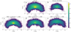 |
Fig. 1. Spacial distribution of stars in the data. Top left panel: number density of stars used in our investigation in the galactocentric Cartesian X–Y plane. This panel contains stars in the 2000 < LZ/ kpc km s−1 < 2600 range. Top right panel: number density of stars within our sample that have global metallicity [M/H] values. Bottom panels: number density of the selected stars in the used angular momentum bins in the X–Y plane. The circled red dot is the location of the Sun in all panels. The bin size for all panels is 200 pc by 200 pc. |
For an investigation of a structure of stars, such as the phase spiral, a velocity-dependant selection will produce a more sharply defined phase spiral than a position-dependent selection because the phase spiral is a dynamical structure (Bland-Hawthorn et al. 2019; Li 2021; Antoja et al. 2023). As noted by Hunt et al. (2021) and Gandhi et al. (2022), samples based on position will contain stars with a wide range of velocities and orbital frequencies because stars with different guiding centre radii will temporarily be close together. This means one will indirectly sample a large part of the Galaxy, which can be useful when addressing other research questions. An example of this is in Bensby et al. (2014) where relatively nearby stars were sampled to map the age and abundance structure of several components of the Milky Way. However, for our purposes, it is more meaningful to group stars in terms of their dynamic properties rather than position.
Here, we do a quick comparison of samples selected by galactocentric position and by angular momentum. Using the Galactic potential from McMillan (2017), we compute the guiding centres for hypothetical stars with LZ = 2200 kpc km s−1 and LZ = 2400 kpc km s−1 to be Rg ≈ 9.5 kpc and Rg ≈ 10.4 kpc, respectively. The Z–VZ phase space for the stars between the galactocentric radii corresponding to these guiding radii are shown in Fig. 2a, and the same for stars in the angular momentum range are shown in Fig. 2b. The phase spiral based on stars in the 9.5 < R / kpc < 10.4 range is visible but less clear, while the phase spiral based on stars in the 2250 < LZ / kpc km s−1 < 2350 range is more prominent. This is because Fig. 2a contains stars that are part of phase spirals with a different appearance, meaning that the stars from one phase spiral fill in the gaps in the pattern made by the other, and vice versa, whereas Fig. 2b mostly contains stars that are part of one single phase spiral, making the pattern clear. Figure 2a contains a total of 1 045 921 stars, while Fig. 2b contains 1 348 886 stars.
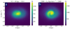 |
Fig. 2. Comparison of phase spirals made of stars selected using different methods. Panel a: number density of stars in the Z–VZ phase plane in the 9.5 < R/ kpc < 10.4 range. Panel b: number density of stars in the Z–VZ phase plane in the 2200 < LZ/ kpc km s−1 < 2400 range. Panel a shows a less clearly defined phase spiral than the one in panel b. |
3. The Gaia phase spiral
Figure 3 shows the density of stars within 5° of the anti-centre direction plotted in the LZ–VZ plane. The thick line is the Galactic disc and the “VZ feature 2” at LZ ≈ 2700 kpc km s−1 is the bifurcation discovered by Gaia Collaboration (2021) and investigated by McMillan et al. (2022), who found that it may be an effect of the passage of the Sagittarius dwarf galaxy. Several other features can be seen, but a particularly clear one that we focus on is the “wrinkle” labelled “VZ feature 1” at LZ ≈ 2300 kpc km s−1 and the apparent overdensity centred on (LZ, VZ) = (2300 kpc km s−1, −20 km s−1). These regions and features are marked lines in Fig. 3. Finding this seemingly isolated overdensity of stars sitting below the thick line was surprising because the stars otherwise show a smooth falloff from the centre in the vertical directions. As we show, the cause for the highlighted overdensity and VZ feature 1 in Fig. 3 seems to be that, in the range 2200 < LZ/ kpc km s−1 < 2400, a higher proportion of the stars are part of the phase spiral, giving the stars in that region an unusual VZ distribution and making phase spiral appear particularly prominent.
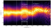 |
Fig. 3. Column-normalised histogram of star number density in the LZ − VZ plane in the Galactic outer disc. The region of interest is marked by solid white lines at LZ = [2200, 2400] kpc km s−1, and by dashed white lines at LZ = 2000 and 2600 kpc km s−1, marking the areas used for comparisons in Figs. 1, 11, and 13. Features mentioned in the text are also marked. The figure contains all stars in our sample with 175° < ϕ < 185°, 12 723 513 in total. |
3.1. Model of the phase spiral
To quantify the properties of the phase spiral as functions of R, ϕ, and LZ, we construct a model inspired by those used by Widmark et al. (2021) and Guo et al. (2022). The model is built by creating a smoothed background from observed data, and then a spiral-shaped perturbation that, when multiplied by the background, recreates the observed distribution of stars in the Z–VZ plane. This way, the spiral can be isolated and quantified. In this model, we compute values for the phase distance r and the phase angle θ using
 (1)
(1)
 (2)
(2)
where S is a scale factor that determines the ratio between the axes and is a free parameter in the model. These coordinates are illustrated in Fig. 4 with a simple diagram. A larger value of S stretches the VZ axis, thus controlling the axis ratio of the spiral; see panel E in Fig. 5. A star experiencing harmonic motion in Z will trace a circle in the phase plane for the right value of S, because S is closely related to the vertical frequency of oscillations in the Galactic disc. We restrict this scale factor to 30 < S < 70, where S is in units of km s−1 kpc−1, as this is the range in which we tend to find stars.
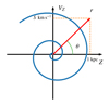 |
Fig. 4. Illustration of the phase-plane coordinates used. r is the phase distance and θ is the phase angle. In this example, θ = 45°. The scale factor S has been chosen such that the r-vector could be drawn with constant length regardless of angle. |
Starting from the discussion of the shape of the phase spiral presented by Guo et al. (2022), we consider the quadratic spiral
 (3)
(3)
where ϕs is the angle of the spiral. These latter authors claim that an Archimedean spiral2 (a = 0, c = 0) fits the data sufficiently well. However, we find that our model fits better when we do not require that c = 0. We can assume a = 0 without loss of generality. As we construct the model, we refer to Fig. 5 for illustrations of the effects of each parameter. Figure 5 contains six panels. Panel A shows the spiral perturbation for a certain set of parameters. Each of the other panels shows the spiral perturbation with one parameter increased and we refer to these panels as we introduce each parameter. We write the equation for the radial distance of the phase spiral as
 (4)
(4)
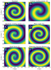 |
Fig. 5. Examples of the effects on the spiral perturbation when changing (increasing) the different parameters in the model. Panel A: spiral perturbation for a certain set of parameters. This is taken as the default for the comparison in this figure. Panel B: spiral perturbation with an increased linear winding parameter. Panel C: spiral perturbation with an increased quadratic winding parameter. We note that the inner part of the spiral is still similar to panel A. Panel D: spiral perturbation with an increased phase angle, rotating it half a revolution. Panel E: spiral perturbation with an increased scale factor, which increases the VZ–Z axis ratio. Panel F: spiral perturbation with the flattening function distance increased, which makes the inner parts less distinct. |
which means
 (5)
(5)
The parameter b is the linear winding term of the spiral. Higher values of b mean the spiral winds slower and moves further in r per turn; see the top-middle panel in Fig. 5. The value of b has to be positive, and by inspection we find it to provide reasonable results between 0.01 and 0.175. c is the quadratic winding term. It has a similar meaning to b, but it does not act equally at all values of r, having a smaller effect close to the middle of the spiral and a greater effect further out; see the top-right panel of Fig. 5. c = 0 means that the spiral is Archimedean and its radius has a constant increase with increasing angle. Here, c has to be positive and, by inspection, we find that we get reasonable results by limiting its upper value to 0.005.
Following Widmark et al. (2021), we take the form of the perturbation to be
 (6)
(6)
where α is a free parameter of the model that defines the amplitude of the phase spiral. This spiral perturbation can have values in the range 1 + α to 1 − α. If α = 0 then the smoothed background is unperturbed by the spiral; if α = 1 there are no stars that are not part of the spiral. We define Δθ as the phase angle relative to the peak of the perturbation as a function of phase distance as
 (7)
(7)
where θ0 is the angle offset, which is a free parameter, giving us
 (8)
(8)
The g(r) term in Eqs. (6) and (8) represents a flattening function that we define below. The innermost part of the phase spiral cannot be accurately fitted with this kind of model because the part of the Galactic disc with low Z-displacement and velocity is subject to small perturbations that wash out the phase spiral. We therefore apply a flattening function called g to reduce the strength of the spiral perturbation in this region. As in Widmark et al. (2021), we use the logistic function (a sigmoid function) for our flattening function. The logistic function has the property that it is bounded by zero and one, and smoothly (exponentially) changes between them, thereby bringing any value into the zero-to-one range in a naturalistic way. We define the flattening function as
 (9)
(9)
where
 (10)
(10)
is the sigmoid function and ρ is the radius parameter of the function, which is a free parameter in the model. The flattening function reduces the impact of the inner part of the spiral by “flattening” it, bringing it closer to one; see the bottom-right panel of Fig. 5. A larger value of ρ means a larger part of the spiral is flattened. By inspection, we find that this value should be less than 0.3, which we apply as a prior.
We also want to reduce the statistical influence of the most distant regions of the phase plane where there are very few stars. Similarly to Widmark et al. (2021), we multiply both data and model by a term that we call mask. We define it as
 (11)
(11)
This mask is applied when evaluating how good the fit is. The mask is the only term in our model that originates in data analysis, and is not some physical property of the phase spiral. We do this because we want the model to correspond to real features. Removing the stars in the outer regions of the phase plane is somewhat arbitrary, but is justified because those regions are very sparse and therefore will only contribute noise.
Combining Eqs. (5), (8), and (9) gives the spiral perturbation as
 (12)
(12)
where α, ρ, θ0, b, and c are free parameters of the model. The prior we use is based on observations of the phase spiral and is chosen in a way that ensures that the sampler converges to the most reasonable solution. The prior uses uniform probabilities for all parameters between the values listed in Table 1. This table also contains a summary of the parameters with their units.
Free parameters in the model of the phase spiral.
3.2. Fitting procedure
The spiral perturbation is found through an algorithm that involves an iterative procedure to create a smooth background (B). With a smooth background, we can define the perturbation that has the parameters of the phase spiral. This background is complicated and changes depending on where in the Galaxy we observe, in part because interstellar extinction hides stars in the plane of the Galactic disc at greater distances, creating a vertical region of lower number density in the middle of the phase plane. Our previous methods were designed to fit a two-dimensional Gaussian to the data for use as a background, but this worked poorly in regions with low star counts. A precursor to the method that we ultimately used involved creating a background based on the data as described below but without any iterative refinement. However, this led to a degree of numerical instability in the results that was resolved by using this iterative method instead.
The procedure for fitting a spiral perturbation to the data is illustrated in Fig. 6 and the letters in this subsection refer to the panels in this figure. The figure contains stars with 8.4 < R / kpc < 10.4 and 165° < ϕ < 195° in the 2200 < LZ / kpc km s−1 < 2400 range. The procedure contains the following steps.
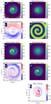 |
Fig. 6. Example of the process from data to fitted model. Panel a: data used for the model, a two-dimensional histogram showing number density consisting of 1 396 320 stars. Panel b: initial background. Panel c: data/initial background. Panel d: extracted spiral perturbation. Panel e: initial fit spiral. Panel f: final background. Panel g: data/final background. Panel h: best fit spiral. Panel i: residuals as computed as: Data (panel a) – Best fit (panel h). See text for details on individual panels. This example consists of stars with 8.4 < R/kpc < 10.4 and 165° < ϕ < 195°. |
1. Collect the data into a two-dimensional number density histogram in the Z − VZ phase plane (panel a). The model uses a bin size of 25 pc by 2 km s−1 except in cases with fewer stars when larger bins are used. For example, Fig. 7 uses bins of  pc by
pc by  km s−1.
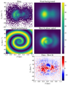 |
Fig. 7. Example of a selection of stars near the edge of our considered area, containing only about 22 000 stars. The sample contains stars with 8 < R/kpc < 12 and 150° < ϕ < 155°. Upper left: phase plane showing strong extinction by dust. Upper right: background produced by the model. Lower left: spiral perturbation produced by the model (this panel does not share the colour bar with the rest). Lower right: best fit. Bottom: residuals computed as Data – Best fit. We can see that even without a clear spiral pattern in the data, the model still produces a convincing spiral and fit. |
2. Create the first background using the observed data (panel b). The background is created from data that have been smoothed by a SciPy Gaussian kernel-density algorithm using Scott’s rule (Scott 1992) to determine the kernel size, and mirrored along the VZ = 0 axis because the background velocity distribution is here assumed to be approximately symmetric.
In panels b and c, we can see that this background still contains some structure from the data and that the spiral pattern in panel c is not clear.
3. Find the spiral perturbation (Eq. (12)) that, when multiplied by this background, fits the data best (panel d). The parameter space is explored and the best fit is found by using a Markov chain Monte Carlo (MCMC)3 approach. To find a fit, we need to define a probability function of a given model that takes the data and our prior into account. Given that we are using an MCMC sampler, we can ignore any multiplicative constants and can say that the relevant value is p, where
 (13)
(13)
where N is the data in the form of number counts for each bin, B is the background, and Pprior is the prior probability. This perturbation is multiplied by the background and the mask (Eq. (11)) and compared to the data (panel e).
4. Divide the data by the spiral perturbation produced in the fit to create an improved background that lacks some of the structure of the initial one (panel f). This new background is smoothed by averaging every pixel with its nearest neighbours (including diagonals) and is no longer necessarily symmetric in VZ. The lack of imposed symmetries makes the smoothing very important as it prevents a solution where the background fits the data directly, bypassing the perturbation and driving the value of α to zero. Removing the requirement of symmetry also allows the entire distribution to drift in VZ. This is not a concern as Dehnen (1999) showed that the VZ distribution of stars in the Galactic disc is not symmetric about VZ = 0. In fact, we see this mismatch between the “symmetric-around-zero” assumption and the data in panel c.
The process described by points 3 and 4 is repeated until the new background no longer provides a better fit. The background converges quickly, usually not improving further after three iterations. The difference this process makes for the background can be seen by comparing panels c and g; we note the clearer spiral pattern in panel g.
5. When making a new background no longer improves the fit, take the final background and perturbation and make the final best fit (panel g). The final parameters are the median of the final samples found by the MCMC sampler.
The quality of the fit can be evaluated by looking at the residuals, which are computed by subtracting the best-fit phase spiral (panel h) from the data (panel a). Panel i shows these residuals. We can see that a weakness in the model is that the fitted spiral has fewer stars in the trough between the wraps of the spiral arm compared to the data as shown by the positive (red) spiral in panel i. This panel also highlights the differences between the mathematically perfect fitted spiral and the natural spiral from the data.
The model is robust and capable of fitting spirals even to regions with relatively few stars. This is because the quality of the fit is judged by how well the smooth background is made to resemble the data, and the spiral perturbation is the way in which it can change this background. In Fig. 7 we show an example of the process when dust severely obscures the sample. The figure contains data in the 8 < R/kpc < 12, 150° < ϕ < 155°, and 2200 < LZ/ kpc km s−1 < 2400 ranges. The model still produces a reasonable fit and provides the parameters of the phase spiral. The residuals shown in the bottom panel display no spiral pattern and have generally low values, further indicating a good fit.
3.3. Rotation of the phase spiral
The online animation 1 shows the phase spiral smoothly transition from stars at ϕ ≈ 210° to stars at ϕ ≈ 150° with bins of 10°. Here the phase spiral can be seen to spin clockwise about half a rotation as we decrease the galactocentric azimuthal angle from ϕ = 150° to ϕ = 210°. At either end of the range, there is a reduction in the number counts of stars in the midplane of the Galactic disc, because interstellar dust blocks our view of these stars. Figure 8 shows the phase spirals at three different Galactic azimuths for stars with 2200 < LZ/ kpc km s−1 < 2400, along with the perturbations fitted to the data. It is evident that the rotation angle of the phase spiral increases (rotating counterclockwise) with Galactic azimuth, changing by roughly 80° over the 30° change in azimuth from ∼165° to ∼195°.
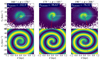 |
Fig. 8. Demonstration of the rotation of the phase spiral with visualisation of how the model found the angles. Upper row: phase spiral at low, medium, and high Galactic azimuth (ϕ) with the angle θ 0, model marked with a red line and θ 0, model = 0 marked with a white dashed line. Lower row: corresponding spiral perturbations fitted to the data with θ 0, model marked with a red line and the measurement distance for θ 0, model marked with a white ring. |
The parameter θ0, which we fit in our model, is not a convenient or particularly helpful description of the rotation of the phase spiral because the angle parameter (θ0) in the model has a degeneracy with the winding parameter (b), and also to a certain extent with the quadratic winding parameter (c), and different sets of these values can produce very similar spirals except in the most central regions, which are removed by the flattening function. Therefore, we describe the rotation of the phase spiral by the angle that maximises Eq. (12) (i.e. Δθ = 0) at a fixed phase distance of r = 500 pc and call this angle θ 0, model. This angle is shown in Fig. 8 with a red line, and the phase distance is shown with a white ring (scaled to the same axis ratio as the phase spiral) in the lower row. The angle 0° is shown with a dashed white line in the upper row. Changing the phase distance at which we take these measurements does not change our results significantly except by changing all angles by some amount. For example, picking r = 150 pc instead would shift all results by ∼120°.
Figure 9 shows the Z-distribution for six different ranges of Galactic azimuth, each of 10° in width, between 150° and 210°, for stars in the 2200 < LZ/ kpc km s−1 < 2400 range. Here, we can clearly see the reduction in the number of stars close to the Galactic plane (Z ≈ 0) at high and low Galactic azimuth. This is because of dust in the plane of the Galactic disc, obscuring the true distribution of stars. Despite this, we see a shift as Galactic azimuth increases with more stars with low Z at low Galactic azimuth than at higher Galactic azimuth, where there are more stars at high Z instead. This is because stars in the phase spiral get pushed to greater Z distances.
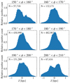 |
Fig. 9. Normalized Z distributions for stars at 2200 < LZ/ kpc km s−1 < 2400 at different Galactic azimuths. We note the seemingly bimodal distribution at Galactic azimuth far from 180°. This is an effect of dust hiding stars in the middle of the Galactic disc. |
Figure 10 shows a map of the rotation angle (θ 0, model) of the phase spiral on a top-down radial grid of the Galactic disc. Three plots are shown, each containing stars in a different angular momentum and galactocentric radial distance range. The left plot contains stars in the 2000 < LZ/ kpc km s−1 < 2200 and 7.5 < R/kpc < 10 range, the middle plot contains stars in the 2200 < LZ/ kpc km s−1 < 2400 and 8.5 < R/kpc < 11 range, and the right plot contains stars in the 2400 < LZ/ kpc km s−1 < 2600 and 9.5 < R/kpc < 12 range, all between 150° and 210° in Galactic azimuth. The zero-point of the rotation angle is set to be zero at the VZ = 0 line at Z > 0 (the positive x-axis as indicated in Fig. 8). In Fig. 10, we see a change in this rotation angle from high to low Galactic azimuth. In the left and middle plots, we see a relatively smooth decrease in rotation angle as Galactic azimuth decreases, changing by about 180° over 60° in the Galactic azimuth. The right panel shows the same trend but the decrease is less smooth. The left panel shows a radial increase in rotation angle by about 40° over 2.5 kpc, while the middle panel shows a radial decrease in this angle by about 70° over 2.5 kpc. The right panel appears to show an increase in angle with radial distance.
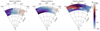 |
Fig. 10. Angle (θ 0, model) of the phase spiral as measured by the model, showing the rotation across the Galactic disc. The plots show data for different regions of the Galaxy as seen from above for the three angular momentum ranges marked in Fig. 3. The colour bar is periodic and the zero point is arbitrary. |
3.4. Amplitude of the phase spiral
Figure 11 shows the Z–VZ phase plane for the three regions marked with lines in Fig. 3. The left and right panel contain stars in the 2000 < LZ/ kpc km s−1 < 2200 and 2400 < LZ/ kpc km s−1 < 2600 ranges, respectively. Both these regions show weak and/or almost dissolved phase-spiral patterns. The middle panel, which corresponds to the 2200 < LZ/ kpc km s−1 < 2400 range, shows a clear, single-armed phase-spiral pattern.
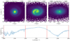 |
Fig. 11. Measurements of the amplitude of the phase spiral as a function of angular momentum. Top: number density of stars at low, medium, and high angular momentum, showing the phase spiral change shape and amplitude. Bottom: amplitude of the phase-spiral pattern as a function of angular momentum. The lines are the same as in Fig. 3. The sample only includes stars that are within 500 pc radially of where a star with the same angular momentum on a circular orbit would be and have a galactocentric radial velocity of less than 22.5 km s−1 in order to restrict the selection to stars on cold orbits. The shaded area shows the 84th and 16th percentiles. |
Our model contains a parameter for the amplitude, or strength, of the phase-spiral pattern (α). The bottom panel of Fig. 11 shows the amplitude of the phase spiral as a function of angular momentum. There is a peak at LZ ≈ 2300 kpc km s−1, which is what we expected from Fig. 3 and the top row of Fig. 11. The shaded region in the plot is between the 84th and 16th percentiles. These are used to show the statistical uncertainties in the model. The systematic uncertainties are expected to be larger. The jagged part between LZ ≈ 2000 kpc km s−1 and 2100 kpc km s−1 is an example of the modelling procedure finding an alternate solution. By visual inspection, we can conclude that the phase spirals found at these points are not the best fits. The line rises at the high end of the plot, indicating another peak at or beyond LZ = 2600 kpc km s−1. This seems to correspond to “VZ feature 2” in Fig. 3 and the bifurcation discussed by McMillan et al. (2022). The data in Fig. 11 are limited to stars with less than |22.5| km s−1 in galactocentric radial velocity, which represents σ/2 (one half standard deviation) of the velocity distribution. In this way, we can select only stars on dynamically cold orbits (close to circular). We do this because we want to compare our results against those of Li & Shen (2020) who investigate the strength of the phase spiral in stars on hot or cold orbits in the solar neighbourhood. The bottom plot contains points based on bins that are 1000 pc by 30°. These bins are centred on the guiding centre radius corresponding to that angular momentum. Because the bins are 30° in width, we are measuring phase spirals with rotational angles over a ∼70° range, as large as that seen in Fig. 8.
Figure 12 shows a map of the amplitude (α) on a top-down radial grid of the Galactic disc. Three plots are shown, each containing stars in a different angular momentum and galactocentric radial distance range, the same as in Fig. 10. The figure shows that the brightest region, with the highest amplitude, is the middle panel with stars in the 2200 < LZ/ kpc km s−1 < 2400 range, which is as we would expect given the results shown in Fig. 11. The figure also shows that the region of the highest amplitude moves outwards with LZ, as well as in each bin. There is a slight trend for the amplitude to decrease at higher and lower Galactic azimuths in the figure. This is believed to be an observational effect that comes from the much greater distances to those areas.
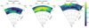 |
Fig. 12. Amplitude (α) of the phase spiral as measured by the model for different regions of the Galaxy as seen from above for the three ranges of angular momentum marked in Fig. 3. The brightness of the plots corresponds to the height of the line in the bottom panel in Fig. 11, showing the change in amplitude across the Galactic disc. |
3.5. Chemical composition of the phase spiral
Figure 13 shows the Z–VZ phase plane coloured by the mean global metallicity for the sample of stars that we have metallicities for in the same three ranges in angular momentum as in Fig. 11. A similar, albeit weaker, spiral pattern can be seen here. We observe that stars in the phase spiral have a slightly higher metallicity than those outside the pattern, indicating a common origin between the stars in the arm of the phase spiral and those in the Galactic thin disc. A clear decreasing trend in mean metallicity with angular momentum can also be seen. The similarities between the spiral patterns in Figs. 11 and 13 are noteworthy but not surprising as stars in the Galactic thin disc are known to have higher metallicity and the phase spiral is assumed to be a perturbation of the Galactic disc, which moves stars away from the midplane. Both figures show stars in the same angular momentum ranges and the same phase-spiral pattern appears. In the left panel, the central region of phase space (the thin disc) shows high [M/H] values. In this panel, an arm of the phase spiral can be seen emerging from the top of this central region at about Z ≈ −300 pc and VZ ≈ 20 km s−1. In the middle panel, a one-armed spiral is visible in stars with mean metallicity of ⟨[M/H]⟩≈ − 0.15 against a background of ⟨[M/H]⟩≈ − 0.22. This panel lacks the high-metallicity region in the centre of the phase plane, and instead the region of highest metallicity is in the arm of the phase spiral. Even the less dense gap between the wraps of the phase-spiral arm is visible as a darker curve near the centre of the phase plane. In contrast to the left panel, this middle panel does not have the highest value in the very centre of the phase plane but shows a small decrease instead. The right panel shows a faint trace of a spiral arm at Z ≈ 500 pc and VZ ≈ −20 km s−1. We note that the colour scale in this panel is shifted slightly towards lower metallicity values in order to bring out the remaining structure.
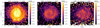 |
Fig. 13. Phase spirals coloured by mean global metallicity at low, medium, and high angular momentum, showing that the spiral pattern is visible. These can be compared to Fig. 11. We note that the rightmost panel has different values on the colour bar. The data are split into the three angular momentum ranges marked in Fig. 3. |
4. Discussion
4.1. Formation
The most established theories for the formation of the phase spiral indicate a single-impact formation mechanism with the Sagittarius dwarf galaxy considered the most popular source of the interaction. However, numerous recent papers are pointing in the opposite direction, and suggest that a single-impact origin scenario is too simple to explain all the observations (e.g. Tremaine et al. 2023; Frankel et al. 2023). The phenomena presented in this paper challenge certain proposed formation mechanisms for the phase spiral. Any model of the phase spiral must be able to reproduce the smoothly changing angle of the phase spiral across a wide range of different Galactic azimuths and radii, which we show in Fig. 10 and our online animation 1. The observed change of the angle would intuitively fit with a single-impact formation scenario.
García-Conde et al. (2022) look at phase spirals in a cosmological simulation and conclude that phase spirals appear even if the interacting satellite galaxies are less massive or more distant than the Sagittarius dwarf galaxy is thought to have been (Niederste-Ostholt et al. 2010). This raises the interesting possibility of these simulations bringing clarity as to whether or not a multi-impact formation scenario can produce a smoothly changing phase spiral. Current simulations do not provide the resolution to answer this question, possibly because they are not set up to do so. While García-Conde et al. (2022) show phase spirals for different Galactic azimuths, the scale is such that the entire area considered in this paper fits in just two bins (see their Figs. 2 and 5 for details).
Knowledge of how the phase spiral shifts across the Galactic disc can be related to the properties of the Galactic disc and the cause of the perturbation. Widmark et al. (2021) used the velocities of stars in the Galactic disc and phase spiral to infer the potential of the Galactic disc, and thereby its mass. Comparing how the phase spiral has propagated through the Galactic disc using results from modelling studies can lead to better constraints for these methods. It should be noted that, as found by many authors (e.g. Gómez et al. 2016; Laporte et al. 2018; Grand et al. 2023), the torque on the Galactic disc caused by the dark-matter wake of a passing satellite galaxy can be significantly stronger than the direct interaction with the satellite galaxy. This means that the connection between the perturbing satellite galaxy and the perturbation in the Galactic disc may not be as simple as some previous idealised models have assumed. Explaining the physics on scales as small as those investigated in the present paper (roughly the area covered by Fig. 10) in the context of a cosmological simulation presents a challenge for the modelling community.
4.2. Hot and cold orbits
Li & Shen (2020) and Bland-Hawthorn et al. (2019) argue that the phase spiral is more clearly defined with stars on dynamically cold (close to circular) orbits than with stars on dynamically hot (far from circular) orbits. Li & Shen (2020) specifically argue that stars on hotter orbits should be excluded from samples used in phase-mixing studies to provide clearer samples. The results of this paper combined with those of Frankel et al. (2023) are in tension with these conclusions. Figure 11 consists of a subset of the full selection of stars; it contains stars on cold orbits by only including stars that are within a 500 pc radius of where a star with the same angular momentum on a circular orbit would be and that have a galactocentric radial velocity of less than |22.5| km s−1, which is approximately σ/2 of the galactocentric radial velocity. The strength of the phase spiral in these kinematically cold stars is similar to that found by Frankel et al. (2023), who show that stars on hot orbits at LZ ≈ 2300 kpc km s−1 still produce a phase spiral with higher amplitude than stars on cold orbits at LZ ≈ 1800 kpc km s−1 (see their Fig. 8 for details). Both results show the same feature, namely a region with a more prominent phase spiral, despite containing separate populations of stars with different dynamics. The conclusion we draw is that the phase spiral and its connection to the Galaxy are more complicated than can be evaluated based on one parameter.
The investigation of the amplitude of the phase-spiral pattern as a function of angular momentum in the range 1250 < LZ/ kpc km s−1 < 2300 conducted by Frankel et al. (2023) is similar to ours but there are some key differences. Their sample consists of stars within a 0.5 kpc cylinder centred on the Sun, meaning that the stars included in this volume with high angular momentum (> 2000 kpc km s−1) are all going to be on relatively dynamically hot orbits. Our sample contains stars whose position and guiding centre are further out, meaning that when considering the high-angular-momentum case, the stars are on dynamically cooler orbits. They show a general increase in amplitude with angular momentum, with the highest peak at LZ ≈ 2350 kpc km s−1 (see their Fig. 8 for details). The bins containing stars with high angular momentum in their sample hold few stars leading to a relatively large scatter in the results. Our results also extend to higher angular momentum, meaning that, in Fig. 11, we can see the dip in amplitude at LZ≈ 2500 kpc km s−1.
The questions posed by Bland-Hawthorn et al. (2019) are still relevant, exploring how various star populations are impacted by the mechanism responsible for the phase spiral. Additionally, the influence on gas is of interest. An intriguing aspect is whether the stars in the phase spiral were formed within it or if they were drawn into it afterward. These questions are mostly outside the scope of this paper, but the answers to them could provide significant insights into the dynamic processes that shape our galaxy.
4.3. Metallicity
Widrow et al. (2012) discovered an asymmetry in the Z-distribution of stars in the Galactic disc, which we now associate with the phase spiral. These authors found that when looking at the number density of stars as (North − South)/(North + South) the result is < 0 at |Z|≈400 pc and > 0 at |Z|≈800 pc. An (2019) analysed this asymmetry further, specifically looking at the metallicity of the stars. These latter authors found that the vertical metallicity distribution is asymmetric in a complicated manner similar to the number density. Our results suggest that the arm of the phase spiral drives stars to greater Z-distances in the region of the Galaxy we study. This would push stars from the Galactic disc vertically away from it, and preferentially in the positive Z-direction (An 2019). We can see this in Fig. 13 where the phase spiral is shown in metallicity and causes the positive Z-side of each plot to be more metal-rich at large distances than the negative Z-side.
Bland-Hawthorn et al. (2019) looked at the difference in the phase spiral when using different cuts in the elemental abundance plane. These authors found that more metal-rich ([Fe/H] > 0.1) stars are concentrated in the central part of the phase spiral. As we can see in Fig. 13, we also see that stars with higher mean metallicity can be found in the centre of the phase spiral for stars with low angular momentum (left panel). The rest of the panels indicate that the most metal-rich stars exist not close to 0 kpc, 0 km s−1 but in the arm of the phase spiral at a distance of ≈0.5 kpc. The conclusion we favour is that these stars were formed in the Galactic thin disc and then perturbed to move out of it. This would explain the asymmetry in the Z-distribution and the concentration of metal-rich stars in the phase spiral.
4.4. Effects of rotation
If the rotation of the phase spiral is not taken into consideration when studying it, some features are at risk of being missed. For example, in Fig. 3, the sample is restricted to stars with Galactic azimuth of 175° < ϕ < 185°; otherwise the feature of interest is not clearly visible. Future authors should be aware of this phenomenon and how it may affect their results.
In Fig. 9 it appears that stars are missing in the centre of the Galactic disc at high or low Galactic azimuth. This is attributed to dust. We also see an asymmetry in the Z distribution when comparing regions at high and low Galactic azimuth. This effect could be caused by the rotation of the phase spiral as it brings the phase spiral arm out of the high-Z region at lower Galactic azimuth. We do not believe this is caused by the warp of the Galactic disc, as the warp only starts being measurable at galactocentric distances greater than those considered here, that is, at about 10 kpc (Cheng et al. 2020). However, the phase spiral and the Galactic warp appear to overlap in certain regions of the Galaxy and are perhaps related. The peak in the phase spiral amplitude is found at LZ = 2300 km kpc s−1, which corresponds to a guiding radius of Rg ≈ 9.9 kpc and reaches a minimum at LZ = 2500 km kpc s−1. This corresponds to Rg ≈ 10.8 kpc, which is within the distance where the Galactic warp starts to be relevant (e.g. Cheng et al. 2020).
5. Summary and conclusions
In this work, we used data from Gaia DR3 to investigate the Gaia phase spiral by making a new model capable of fitting several of its key characteristics. We used a sample of stars with measured radial velocities to get full three-dimensional information on both their position and velocity, a sample of about 31.5 million stars. Using our model, we can determine the rate of rotation of the phase spiral with Galactic azimuth and the amplitude of the phase spiral as a function of angular momentum. We find that, for the data we explore, the phase spiral rotates with Galactic azimuth. We find a peak in the amplitude of the phase spiral at LZ ≈ 2300 km kpc s−1, which manifests as a very clear phase-spiral pattern in number density when using only stars with similar angular momentum.
Our main findings in this paper can be summarised as follows:
-
The phase spiral changes orientation along both Galactic radial distance and Galactic azimuth, and it rotates at a rate which is three times the rate of the azimuthal angle, a rate of ∼180° per 60° Galactic azimuth for stars with angular momenta from 2000 km kpc s−1 to 2400 km kpc s−1, corresponding to orbits typically found outside the Sun’s position in the Galaxy.
-
The amplitude of the phase-spiral pattern changes with angular momentum with a peak at about 2300 ± 100 kpc km s−1, producing a substantially clearer spiral pattern in number density.
-
The stars in the phase-spiral arm are chemically very similar to those in the Z-centre of the Galactic disc. This indicates that the stars in the phase spiral originally belonged to the Galactic thin disc.
-
We can confirm the conclusions of An (2019) and Bland-Hawthorn et al. (2019) that the Z-asymmetry of the metallicity gradient of the Galaxy is caused by the metal-rich arm of the phase spiral pushing such stars to greater Z-positions.
We find the reason for the change in the LZ–VZ distribution between the solid lines in Fig. 3, that is, the overdensity seen below the thick line, to be linked to the phase spiral. In Fig. 11, we show the number density of the phase spiral in three regions in the top row. Here we can see that the central panel, which contains stars in the 2200 km kpc s−1 to 2400 km kpc s−1 range, shows a clearer and more defined spiral pattern. The bottom of the same figure shows the amplitude of the phase spiral as measured by the model. Here we also see that the phase spiral is strongest in the 2200 km kpc s−1 to 2400 km kpc s−1 range. The point at which the central line in Fig. 3 is raised to about 15 km s−1, at the “VZ feature 1”, corresponds to when the phase spiral arm first shows negative Z-values, when considering the phase spiral as going from the centre outwards. The overdensity at −20 km s−1 corresponds to when the spiral arm turns back to the positive Z-values.
By combining the data from Gaia with those coming from the soon-to-be operational spectrographs 4MOST (Bensby et al. 2019; Chiappini et al. 2019) and WEAVE (Jin et al. 2023), more light will be shed on the origins of the phase spiral by revealing detailed chemical abundances for millions of stars in all parts of the Milky Way.
Movies
Animation 1 (phase_spiral_animation1) Access Supplementary Material
Animation 2 (phase_spiral_animation2) Access Supplementary Material
Animation 3 (phase_spiral_animation3) Access Supplementary Material
An Archimedean spiral is a spiral with a linear relation between angle and radial distance. Expressed in polar coordinates the spiral traces r = bϕs.
The model is implemented in Python using the package emcee (Foreman-Mackey et al. 2013) as an MCMC sampler.
Acknowledgments
P.M. gratefully acknowledges support from project grants from the Swedish Research Council (Vetenskaprådet, Reg: 2017-03721; 2021-04153). T.B. and S.A. acknowledge support from project grant No. 2018-04857 from the Swedish Research Council. Some of the computations in this project were completed on computing equipment bought with a grant from The Royal Physiographic Society in Lund. This work has made use of data from the European Space Agency (ESA) mission Gaia (https://www.cosmos.esa.int/gaia), processed by the Gaia Data Processing and Analysis Consortium (DPAC, https://www.cosmos.esa.int/web/gaia/dpac/consortium). Funding for the DPAC has been provided by national institutions, in particular the institutions participating in the Gaia Multilateral Agreement. This research has made use of NASA’s Astrophysics Data System. This paper made use of the following software packages for Python, Numpy (Harris et al. 2020), AstroPy (Astropy Collaboration 2022), emcee (Foreman-Mackey et al. 2013), SciPy (Virtanen et al. 2020).
References
- Abolfathi, B., Aguado, D. S., Aguilar, G., et al. 2018, ApJS, 235, 42 [NASA ADS] [CrossRef] [Google Scholar]
- Alves, J., Zucker, C., Goodman, A. A., et al. 2020, Nature, 578, 237 [NASA ADS] [CrossRef] [Google Scholar]
- An, D. 2019, ApJ, 878, L31 [NASA ADS] [CrossRef] [Google Scholar]
- Antoja, T., Helmi, A., Romero-Gómez, M., et al. 2018, Nature, 561, 360 [Google Scholar]
- Antoja, T., Ramos, P., García-Conde, B., et al. 2023, A&A, 673, A115 [NASA ADS] [CrossRef] [EDP Sciences] [Google Scholar]
- Astropy Collaboration (Price-Whelan, A. M., et al.) 2022, ApJ, 935, 167 [NASA ADS] [CrossRef] [Google Scholar]
- Bailer-Jones, C. A. L., Rybizki, J., Fouesneau, M., Demleitner, M., & Andrae, R. 2021, AJ, 161, 147 [Google Scholar]
- Belokurov, V., Erkal, D., Evans, N. W., Koposov, S. E., & Deason, A. J. 2018, MNRAS, 478, 611 [Google Scholar]
- Bennett, M., & Bovy, J. 2019, MNRAS, 482, 1417 [NASA ADS] [CrossRef] [Google Scholar]
- Bennett, M., Bovy, J., & Hunt, J. A. S. 2022, ApJ, 927, 131 [NASA ADS] [CrossRef] [Google Scholar]
- Bensby, T., Feltzing, S., & Oey, M. S. 2014, A&A, 562, A71 [NASA ADS] [CrossRef] [EDP Sciences] [Google Scholar]
- Bensby, T., Bergemann, M., Rybizki, J., et al. 2019, The Messenger, 175, 35 [NASA ADS] [Google Scholar]
- Binney, J., & Schönrich, R. 2018, MNRAS, 481, 1501 [Google Scholar]
- Bland-Hawthorn, J., & Tepper-García, T. 2021, MNRAS, 504, 3168 [CrossRef] [Google Scholar]
- Bland-Hawthorn, J., Sharma, S., Tepper-Garcia, T., et al. 2019, MNRAS, 486, 1167 [NASA ADS] [CrossRef] [Google Scholar]
- Buder, S., Asplund, M., Duong, L., et al. 2018, MNRAS, 478, 4513 [Google Scholar]
- Cheng, X., Anguiano, B., Majewski, S. R., et al. 2020, ApJ, 905, 49 [Google Scholar]
- Chiappini, C., Minchev, I., Starkenburg, E., et al. 2019, The Messenger, 175, 30 [NASA ADS] [Google Scholar]
- Darling, K., & Widrow, L. M. 2019, MNRAS, 484, 1050 [CrossRef] [Google Scholar]
- Darragh-Ford, E., Hunt, J. A. S., Price-Whelan, A. M., & Johnston, K. V. 2023, ApJ, 955, 74 [NASA ADS] [CrossRef] [Google Scholar]
- Dehnen, W. 1999, ASP Conf. Ser., 182, 297 [NASA ADS] [Google Scholar]
- Drimmel, R., & Poggio, E. 2018, Res. Notes Am. Astron. Soc., 2, 210 [Google Scholar]
- Foreman-Mackey, D., Hogg, D. W., Lang, D., & Goodman, J. 2013, PASP, 125, 306 [Google Scholar]
- Frankel, N., Bovy, J., Tremaine, S., & Hogg, D. W. 2023, MNRAS, 521, 5917 [NASA ADS] [CrossRef] [Google Scholar]
- Freeman, K., & Bland-Hawthorn, J. 2002, ARA&A, 40, 487 [Google Scholar]
- Gaia Collaboration (Prusti, T., et al.) 2016, A&A, 595, A1 [NASA ADS] [CrossRef] [EDP Sciences] [Google Scholar]
- Gaia Collaboration (Brown, A. G. A., et al.) 2018, A&A, 616, A1 [NASA ADS] [CrossRef] [EDP Sciences] [Google Scholar]
- Gaia Collaboration (Brown, A. G. A., et al.) 2021, A&A, 649, A1 [NASA ADS] [CrossRef] [EDP Sciences] [Google Scholar]
- Gaia Collaboration (Vallenari, A., et al.) 2023, A&A, 674, A1 [NASA ADS] [CrossRef] [EDP Sciences] [Google Scholar]
- Gandhi, S. S., Johnston, K. V., Hunt, J. A. S., et al. 2022, ApJ, 928, 80 [NASA ADS] [CrossRef] [Google Scholar]
- García-Conde, B., Roca-Fàbrega, S., Antoja, T., Ramos, P., & Valenzuela, O. 2022, MNRAS, 510, 154 [Google Scholar]
- Gómez, F. A., White, S. D. M., Marinacci, F., et al. 2016, MNRAS, 456, 2779 [Google Scholar]
- Grand, R. J. J., Pakmor, R., Fragkoudi, F., et al. 2023, MNRAS, 524, 801 [NASA ADS] [CrossRef] [Google Scholar]
- GRAVITY Collaboration (Abuter, R., et al.) 2018, A&A, 615, L15 [NASA ADS] [CrossRef] [EDP Sciences] [Google Scholar]
- Guo, R., Shen, J., Li, Z.-Y., Liu, C., & Mao, S. 2022, ApJ, 936, 103 [NASA ADS] [CrossRef] [Google Scholar]
- Harris, C. R., Millman, K. J., van der Walt, S. J., et al. 2020, Nature, 585, 357 [NASA ADS] [CrossRef] [Google Scholar]
- Helmi, A., Veljanoski, J., Breddels, M. A., Tian, H., & Sales, L. V. 2017, A&A, 598, A58 [NASA ADS] [CrossRef] [EDP Sciences] [Google Scholar]
- Helmi, A., Babusiaux, C., Koppelman, H. H., et al. 2018, Nature, 563, 85 [Google Scholar]
- Hunt, J. A. S., Stelea, I. A., Johnston, K. V., et al. 2021, MNRAS, 508, 1459 [NASA ADS] [CrossRef] [Google Scholar]
- Hunt, J. A. S., Price-Whelan, A. M., Johnston, K. V., & Darragh-Ford, E. 2022, MNRAS, 516, L7 [NASA ADS] [CrossRef] [Google Scholar]
- Ibata, R. A., Gilmore, G., & Irwin, M. J. 1994, Nature, 370, 194 [Google Scholar]
- Jin, S., Trager, S. C., Dalton, G. B., et al. 2023, MNRAS, in press https://doi.org/10.1093/mnras/stad557 [Google Scholar]
- Laporte, C. F. P., Johnston, K. V., Gómez, F. A., Garavito-Camargo, N., & Besla, G. 2018, MNRAS, 481, 286 [Google Scholar]
- Laporte, C. F. P., Minchev, I., Johnston, K. V., & Gómez, F. A. 2019, MNRAS, 485, 3134 [Google Scholar]
- Li, Z.-Y. 2021, ApJ, 911, 107 [NASA ADS] [CrossRef] [Google Scholar]
- Li, Z.-Y., & Shen, J. 2020, in Galactic Dynamics in the Era of Large Surveys, eds. M. Valluri, & J. A. Sellwood, 353, 10 [NASA ADS] [Google Scholar]
- Massari, D., Breddels, M. A., Helmi, A., et al. 2018, Nat. Astron., 2, 156 [Google Scholar]
- McMillan, P. J. 2017, MNRAS, 465, 76 [NASA ADS] [CrossRef] [Google Scholar]
- McMillan, P. J., Petersson, J., Tepper-Garcia, T., et al. 2022, MNRAS, 516, 4988 [NASA ADS] [CrossRef] [Google Scholar]
- Niederste-Ostholt, M., Belokurov, V., Evans, N. W., & Peñarrubia, J. 2010, ApJ, 712, 516 [NASA ADS] [CrossRef] [Google Scholar]
- Recio-Blanco, A., de Laverny, P., Palicio, P. A., et al. 2023, A&A, 674, A29 [NASA ADS] [CrossRef] [EDP Sciences] [Google Scholar]
- Reid, M. J., & Brunthaler, A. 2004, ApJ, 616, 872 [Google Scholar]
- Scott, D. W. 1992, Multivariate Density Estimation (New York, NY: Wiley) [Google Scholar]
- Tremaine, S., Frankel, N., & Bovy, J. 2023, MNRAS, 521, 114 [NASA ADS] [CrossRef] [Google Scholar]
- Virtanen, P., Gommers, R., Oliphant, T. E., et al. 2020, Nat. Methods, 17, 261 [Google Scholar]
- Wang, C., Huang, Y., Yuan, H. B., et al. 2019, ApJ, 877, L7 [NASA ADS] [CrossRef] [Google Scholar]
- Widmark, A., Laporte, C. F. P., de Salas, P. F., & Monari, G. 2021, A&A, 653, A86 [NASA ADS] [CrossRef] [EDP Sciences] [Google Scholar]
- Widmark, A., Hunt, J. A. S., Laporte, C. F. P., & Monari, G. 2022a, A&A, 663, A16 [NASA ADS] [CrossRef] [EDP Sciences] [Google Scholar]
- Widmark, A., Widrow, L. M., & Naik, A. 2022b, A&A, 668, A95 [NASA ADS] [CrossRef] [EDP Sciences] [Google Scholar]
- Widrow, L. M. 2023, MNRAS, 522, 477 [NASA ADS] [CrossRef] [Google Scholar]
- Widrow, L. M., Gardner, S., Yanny, B., Dodelson, S., & Chen, H.-Y. 2012, ApJ, 750, L41 [Google Scholar]
- Xu, Y., Liu, C., Tian, H., et al. 2020, ApJ, 905, 6 [NASA ADS] [CrossRef] [Google Scholar]
Appendix A: Further data
Figure A.1 shows the phase spiral for 12 different ranges of Galactic azimuth, each 5° in width, between 150° and 210°, for stars in the 2000 < LZ/ kpc km s−1 < 2200 range. Each panel has the rotation angle (θ 0, model) marked with a red line. Figures A.2 and A.3 show the same for the 2200 < LZ/ kpc km s−1 < 2400 and 2400 < LZ/ kpc km s−1 < 2600 ranges respectively. The angle of the phase spiral changes with Galactic azimuth in this figure as well, rotating about 200° over an azimuth range of about 55°. The phase spiral is most clearly seen around ϕ = 180° and becomes less prominent in both azimuthal directions as the number of stars in our data decreases.
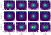 |
Fig. A.1. Phase spirals and fitted spiral perturbations at different values for Galactic azimuth (ϕ) in the 2000 < LZ/ kpc km s−1 < 2200 range. The measured angle of the phase spiral is marked with a red line. The azimuthal range of the stars is marked with text in the right panels. This figure shows how we can use the model to determine the angle of the phase spiral, even in regions where the data are of lower quality due to extinction by dust. |
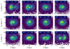 |
Fig. A.2. Phase spirals and fitted spiral perturbations at different values for Galactic azimuth (ϕ) in the 2200 < LZ/ kpc km s−1 < 2400 range. The measured angle of the phase spiral is marked with a red line. The azimuthal range of the stars is marked with text in the right panels. |
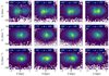 |
Fig. A.3. Phase spirals and fitted spiral perturbations at different values for Galactic azimuth (ϕ) in the 2400 < LZ/ kpc km s−1 < 2600 range. The measured angle of the phase spiral is marked with a red line. The azimuthal range of the stars is marked with text in the right panels. |
Animations of the phase spiral over a range of Galactic azimuths —similar to that in the main paper— for stars at lower and higher angular momentum are available online (animations 2 and 3).
All Tables
All Figures
|
Fig. 1. Spacial distribution of stars in the data. Top left panel: number density of stars used in our investigation in the galactocentric Cartesian X–Y plane. This panel contains stars in the 2000 < LZ/ kpc km s−1 < 2600 range. Top right panel: number density of stars within our sample that have global metallicity [M/H] values. Bottom panels: number density of the selected stars in the used angular momentum bins in the X–Y plane. The circled red dot is the location of the Sun in all panels. The bin size for all panels is 200 pc by 200 pc. |
| In the text | |
|
Fig. 2. Comparison of phase spirals made of stars selected using different methods. Panel a: number density of stars in the Z–VZ phase plane in the 9.5 < R/ kpc < 10.4 range. Panel b: number density of stars in the Z–VZ phase plane in the 2200 < LZ/ kpc km s−1 < 2400 range. Panel a shows a less clearly defined phase spiral than the one in panel b. |
| In the text | |
|
Fig. 3. Column-normalised histogram of star number density in the LZ − VZ plane in the Galactic outer disc. The region of interest is marked by solid white lines at LZ = [2200, 2400] kpc km s−1, and by dashed white lines at LZ = 2000 and 2600 kpc km s−1, marking the areas used for comparisons in Figs. 1, 11, and 13. Features mentioned in the text are also marked. The figure contains all stars in our sample with 175° < ϕ < 185°, 12 723 513 in total. |
| In the text | |
|
Fig. 4. Illustration of the phase-plane coordinates used. r is the phase distance and θ is the phase angle. In this example, θ = 45°. The scale factor S has been chosen such that the r-vector could be drawn with constant length regardless of angle. |
| In the text | |
|
Fig. 5. Examples of the effects on the spiral perturbation when changing (increasing) the different parameters in the model. Panel A: spiral perturbation for a certain set of parameters. This is taken as the default for the comparison in this figure. Panel B: spiral perturbation with an increased linear winding parameter. Panel C: spiral perturbation with an increased quadratic winding parameter. We note that the inner part of the spiral is still similar to panel A. Panel D: spiral perturbation with an increased phase angle, rotating it half a revolution. Panel E: spiral perturbation with an increased scale factor, which increases the VZ–Z axis ratio. Panel F: spiral perturbation with the flattening function distance increased, which makes the inner parts less distinct. |
| In the text | |
|
Fig. 6. Example of the process from data to fitted model. Panel a: data used for the model, a two-dimensional histogram showing number density consisting of 1 396 320 stars. Panel b: initial background. Panel c: data/initial background. Panel d: extracted spiral perturbation. Panel e: initial fit spiral. Panel f: final background. Panel g: data/final background. Panel h: best fit spiral. Panel i: residuals as computed as: Data (panel a) – Best fit (panel h). See text for details on individual panels. This example consists of stars with 8.4 < R/kpc < 10.4 and 165° < ϕ < 195°. |
| In the text | |
|
Fig. 7. Example of a selection of stars near the edge of our considered area, containing only about 22 000 stars. The sample contains stars with 8 < R/kpc < 12 and 150° < ϕ < 155°. Upper left: phase plane showing strong extinction by dust. Upper right: background produced by the model. Lower left: spiral perturbation produced by the model (this panel does not share the colour bar with the rest). Lower right: best fit. Bottom: residuals computed as Data – Best fit. We can see that even without a clear spiral pattern in the data, the model still produces a convincing spiral and fit. |
| In the text | |
|
Fig. 8. Demonstration of the rotation of the phase spiral with visualisation of how the model found the angles. Upper row: phase spiral at low, medium, and high Galactic azimuth (ϕ) with the angle θ 0, model marked with a red line and θ 0, model = 0 marked with a white dashed line. Lower row: corresponding spiral perturbations fitted to the data with θ 0, model marked with a red line and the measurement distance for θ 0, model marked with a white ring. |
| In the text | |
|
Fig. 9. Normalized Z distributions for stars at 2200 < LZ/ kpc km s−1 < 2400 at different Galactic azimuths. We note the seemingly bimodal distribution at Galactic azimuth far from 180°. This is an effect of dust hiding stars in the middle of the Galactic disc. |
| In the text | |
|
Fig. 10. Angle (θ 0, model) of the phase spiral as measured by the model, showing the rotation across the Galactic disc. The plots show data for different regions of the Galaxy as seen from above for the three angular momentum ranges marked in Fig. 3. The colour bar is periodic and the zero point is arbitrary. |
| In the text | |
|
Fig. 11. Measurements of the amplitude of the phase spiral as a function of angular momentum. Top: number density of stars at low, medium, and high angular momentum, showing the phase spiral change shape and amplitude. Bottom: amplitude of the phase-spiral pattern as a function of angular momentum. The lines are the same as in Fig. 3. The sample only includes stars that are within 500 pc radially of where a star with the same angular momentum on a circular orbit would be and have a galactocentric radial velocity of less than 22.5 km s−1 in order to restrict the selection to stars on cold orbits. The shaded area shows the 84th and 16th percentiles. |
| In the text | |
|
Fig. 12. Amplitude (α) of the phase spiral as measured by the model for different regions of the Galaxy as seen from above for the three ranges of angular momentum marked in Fig. 3. The brightness of the plots corresponds to the height of the line in the bottom panel in Fig. 11, showing the change in amplitude across the Galactic disc. |
| In the text | |
|
Fig. 13. Phase spirals coloured by mean global metallicity at low, medium, and high angular momentum, showing that the spiral pattern is visible. These can be compared to Fig. 11. We note that the rightmost panel has different values on the colour bar. The data are split into the three angular momentum ranges marked in Fig. 3. |
| In the text | |
|
Fig. A.1. Phase spirals and fitted spiral perturbations at different values for Galactic azimuth (ϕ) in the 2000 < LZ/ kpc km s−1 < 2200 range. The measured angle of the phase spiral is marked with a red line. The azimuthal range of the stars is marked with text in the right panels. This figure shows how we can use the model to determine the angle of the phase spiral, even in regions where the data are of lower quality due to extinction by dust. |
| In the text | |
|
Fig. A.2. Phase spirals and fitted spiral perturbations at different values for Galactic azimuth (ϕ) in the 2200 < LZ/ kpc km s−1 < 2400 range. The measured angle of the phase spiral is marked with a red line. The azimuthal range of the stars is marked with text in the right panels. |
| In the text | |
|
Fig. A.3. Phase spirals and fitted spiral perturbations at different values for Galactic azimuth (ϕ) in the 2400 < LZ/ kpc km s−1 < 2600 range. The measured angle of the phase spiral is marked with a red line. The azimuthal range of the stars is marked with text in the right panels. |
| In the text | |
Current usage metrics show cumulative count of Article Views (full-text article views including HTML views, PDF and ePub downloads, according to the available data) and Abstracts Views on Vision4Press platform.
Data correspond to usage on the plateform after 2015. The current usage metrics is available 48-96 hours after online publication and is updated daily on week days.
Initial download of the metrics may take a while.