| Issue |
A&A
Volume 673, May 2023
|
|
|---|---|---|
| Article Number | A115 | |
| Number of page(s) | 16 | |
| Section | Galactic structure, stellar clusters and populations | |
| DOI | https://doi.org/10.1051/0004-6361/202245518 | |
| Published online | 16 May 2023 | |
The phase spiral in Gaia DR3
1
Departament de Física Quàntica i Astrofísica (FQA), Universitat de Barcelona (UB), c. Martí i Franquès, 1, 08028 Barcelona, Spain
e-mail: This email address is being protected from spambots. You need JavaScript enabled to view it.
2
Institut de Ciències del Cosmos (ICCUB), Universitat de Barcelona (UB), c. Martí i Franquès, 1 08028 Barcelona, Spain
3
Institut d’Estudis Espacials de Catalunya (IEEC), c. Gran Capità, 2-4, 08034 Barcelona, Spain
4
(Research Affiliate) National Astronomical Observatory of Japan, Mitaka-shi, Tokyo 181-8588, Japan
5
Departamento de Física de la Tierra y Astrofísica, Fac. CC. Físicas, Universidad Complutense de Madrid, Plaza de las Ciencias, 1, Madrid 28040, Spain
6
GEPI, Observatoire de Paris, Université PSL, CNRS, 5 Place Jules Janssen, 92190 Meudon, France
Received:
21
November
2022
Accepted:
7
March
2023
Abstract
Aims. We aim to study the phase spiral in the Milky Way (MW) disc with data from the third data release of Gaia (DR3) and use it as an inference tool to decipher the late-time evolution of the Galaxy.
Methods. We used an edge-detection algorithm to find the border of the phase spiral, allowing us to robustly quantify its shape at different positions and for different selections. We calculated the time of onset of the phase-mixing by determining the different turns of the phase spiral and using the vertical frequencies from commonly used models of the gravitational potential of the MW.
Results. We find that the phase spiral extends down to −1.2 kpc in height below the plane (about 3–5 scale heights of the thin disc) and beyond ±50 km s−1 in VZ. We see a secondary branch mostly at positive vertical velocities when coloured by azimuthal velocity and in the counts projection. We also find complex variations of the phase spirals with angular momentum and azimuth. All these findings are possible evidence of multiple perturbations (from different times or from different perturbers) and/or of the complexity of the phase-mixing process. We detect the phase spiral from 6 to 11 kpc from the Galactic centre and find signatures of vertical asymmetries 1–2 kpc beyond this range. We measure small but clear variations with azimuth. When we determine the phase mixing times from the phase spiral at different angular momenta and using the different spiral turns (at different Z), we obtain inconsistent times with systematic differences (times increasing with |LZ| and with |Z|). Our determinations are mostly in the range of [0.3–0.9] Gyr, with an average of 0.5 Gyr. The inconsistencies do not change when using different commonly used potential models for the MW, different stellar distances, or frequencies for different kinetic temperatures; they could stem from the inconsistency of the assumed gravitational potentials with the true MW, and from oversimplification of the modelling, in particular where self-gravity is neglected or where multiple perturbations and/or interference with other processes are not considered.
Conclusions. The wealth of information provided by the new Gaia DR3 data should encourage us to make progress in crucial modelling aspects of the disc dynamics, such as non-equilibrium, self-gravity, propagation of different types of bending waves, and interactions between different mechanisms. Such advancements could finally enable us to establish the origin of the phase spiral and its relation to the Sagittarius dwarf galaxy.
Key words: Galaxy: kinematics and dynamics / Galaxy: evolution / Galaxy: disk / Galaxy: structure / galaxies: interactions
© The Authors 2023
 Open Access article, published by EDP Sciences, under the terms of the Creative Commons Attribution License (https://creativecommons.org/licenses/by/4.0), which permits unrestricted use, distribution, and reproduction in any medium, provided the original work is properly cited.
This article is published in open access under the Subscribe to Open model. This email address is being protected from spambots. You need JavaScript enabled to view it. to support open access publication.
1. Introduction
The snail shell or phase spiral that appeared in the vertical projection of the phase space (Antoja et al. 2018, hereafter A18) in the data of the second data release of the Gaia mission (DR2; Gaia Collaboration 2016, 2018) informed us about a process of phase mixing that began following a perturbation from which the Milky Way (MW) is still recovering. These findings provided further details about the vertical asymmetries discovered by Widrow et al. (2012) and Williams et al. (2013).
Later we learned that the phase spiral shrinks in the Z direction when moving from the outer to the inner parts of the Galaxy (Laporte et al. 2019; Wang et al. 2019) as expected, that it is more prominent for cold orbits (Bland-Hawthorn et al. 2019; Li & Shen 2020), that it shows mild changes with azimuth (e.g., slightly different density of stars along the phase spiral; Bland-Hawthorn et al. 2019), and that it is present in different age ranges (Tian et al. 2018; Laporte et al. 2019; Bland-Hawthorn et al. 2019), even in samples younger than 0.5 Gyr. The fanning of the phase spiral when colour coded according to the azimuthal velocity can be explained by the different vertical frequencies at different angular momenta (A18).
As for the causes of the phase spiral, most studies favour the hypothesis that it is due to the approach of the Sagittarius dwarf galaxy (A18, Binney & Schönrich 2018; Laporte et al. 2018; Bland-Hawthorn & Tepper-García 2021; Banik et al. 2022). However, there are several complex aspects involved that remain to be fully understood, such as the effects of self-gravity discussed by Darling & Widrow (2019), the mass of Sagittarius needed to activate phase spirals (e.g., see discussions in García-Conde et al. 2022; Bennett et al. 2022), or which Sagittarius pericentre/s excited the phase spiral. Alternatively, the phase spiral found in the data of DR2 might have been caused by bending waves sparked by the buckling of the bar (Khoperskov et al. 2019) or the impact of several (dark) subhalos (Chequers et al. 2018; Tremaine et al. 2023), and its formation and evolution may have been helped by the wake of the halo excited by satellite passages (Grand et al. 2022).
The shape of the phase spiral offers a way to constrain both the perturber and the potential of the Galaxy through the vertical orbital frequencies of the stars. In A18, we assumed a set of frequencies of the MW and derived a perturbation time of 300–900 Myr. Ideally, both the potential and the perturbation times can be fitted at the same time as in Widmark et al. (2021), although these two quantities appear to be degenerate in the fit.
In addition, the phase spiral alerted us to the fact that the assumption of a Galaxy in equilibrium may have biased certain determinations, such as that of the quantity of dark matter through the Jeans equations (Haines et al. 2019; Chrobáková et al. 2020). Furthermore, the vertical perturbations that led to the phase spiral might have other important consequences for the Galaxy. For example, they may have come accompanied by disturbances in the other components of phase space and/or changes in the morphology of the MW (Laporte et al. 2018; Bland-Hawthorn & Tepper-García 2021; Antoja et al. 2022), as proposed earlier, for example, by Younger et al. (2008) and Purcell et al. (2011). The event might also be related to different episodes of strong star formation in the disc discovered with Gaia data as well (Mor et al. 2019; Ruiz-Lara et al. 2020).
The publication of the third Gaia data release (DR3; Gaia Collaboration 2023c) offers a new opportunity to explore the phase spiral across the disc and its stellar composition through a better selection of populations. For example, Gaia Collaboration (2023b) showed that the phase spiral also appears when painted by metallicity, because of the correlation between metallicity and angular momentum. Recently, Hunt et al. (2022) discovered double spirals in the inner parts of the Galaxy and demonstrated that they could be due to breathing modes excited by internal structures such as the bar (but not necessarily a buckling bar) and/or by an external perturber, in a similar way to the double spirals from their simulations (Hunt et al. 2021).
Here, we explore the phase spiral with Gaia DR3 and try to carry out a new determination of the perturbation time. In Sect. 2, we describe the data selection and corrections. In Sect. 3, we explore the local phase spiral, now with many more stars and with measurements of higher precision (Sect. 3.1); we describe the method we use to detect the phase spiral and obtain its exact position in the Z–VZ plane (Sect. 3.2); and we further explore its spatial variations as functions of radius and angular momentum (Sects. 3.3 and 3.4) as well as azimuth (Sect. 3.5). In Sect. 4, we provide a fit to the time of perturbation in a similar way to A18 but now considering the phase spiral at different angular momenta, which reveals interesting inconsistencies. In Sect. 5, we discuss our findings and present our conclusions.
2. Data
We used data from Gaia DR3 (Gaia Collaboration 2023c). We selected stars with available radial velocity and applied the following quality selections: (1) Astrometric quality selection: RUWE < 1.4, (2) selection in parallax quality: parallax_over_error > 5, and (3) selection of non-spurious solutions (Rybizki et al. 2022): fidelity_v2 > 0.5.
We used distances from StarHorse (hereafter SH, Anders et al. 2022) by default. We also used the photogeometric distances from Bailer-Jones et al. (2021, hereafter BJ) for comparison (finding no important differences in our results) and also to test the robustness of the detections (see Sect. 3.3). In addition, we applied the following correction to the line-of-sight velocity for stars with grvs_mag ≥ 11 and rv_template_teff < 8500 (Katz et al. 2023):
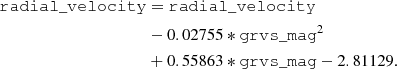 (1)
(1)
As discussed in Blomme et al. (2023), a correction is also necessary for the stars with 8500 ≤ rv_template_teff ≤ 14 500 K and 6 ≤ grvs_mag ≤ 12 but after the correction there is still a residual bias of a few km s−1. As these stars are not very numerous, in our samples, we keep only stars with rv_template_teff < 8500 K.
After all the above selections, the final sample with SH distances contains 25 397 569 stars, while that with BJ distances contains 26 407 121 stars. The queries used to retrieve the data from the Gaia archive are presented in Appendix A. In Appendix B, we compare the two sets of distances and in Appendixes C and D we discuss the effects of distance errors and biases and the selection function, respectively, on the detected phase spiral.
We transformed the Gaia observables into usual cylindrical phase-space coordinates. To this end, we used R0 = 8.277 kpc (Gravity Collaboration 2022), Z⊙ = 0.0208 kpc (Bennett & Bovy 2019), and U⊙ = 9.3, V⊙ + Vc(R0) = 251.5 and W⊙ = 8.59 km s−1 from the combination of the proper motion of SagA* from Reid & Brunthaler 2020 and its radial velocity from Gravity Collaboration (2022), where U, V, and W are the usual heliocentric Cartesian velocities and Vc(R0) is the circular velocity curve at the position of the Sun. Our reference system is a right-handed one with ϕ < 0 in the sense of rotation, and therefore also Vϕ < 0 for most of the stars. We set the origin at the azimuth of the Sun (ϕ⊙ = 0).
3. The phase spiral in DR3
3.1. The local phase spiral
In Fig. 1 we look at the local phase spiral in the Z–VZ plane by selecting stars with R0 − 0.1 kpc < R < R0 + 0.1 kpc and −20 < ϕ < 20deg. This large range in ϕ is justified by the phase spiral not changing significantly with ϕ compared to R, as we see below. In A18, with DR2 data, only the radial cut was performed, making a sample of 935 590 stars. Here, we have a local sample with 2 328 004 stars. We note that we have increased the range in Z and VZ of the panels in Fig. 1 compared to our previous work. We used bins with a size of ΔZ = 0.02 kpc and ΔVZ = 1 km s−1. The three panels of Fig. 1 (counts and coloured by median VR and by median Vϕ, respectively) now show a sharper signal. For example, the middle panel presents defined spiral segments of different VR, including two blue segments in the upper left part. In the right panel, the phase spiral has a secondary branch at 50 km s−1. While this could be partially observed in DR2 (A18, Laporte et al. 2019), now it is seen to be clearly separate from the other (main) spiral. This branching now reaches Z = −1.2 kpc, that is, between about three and five scale heights of the thin disc (taken to be 220–450 pc, Bland-Hawthorn & Gerhard 2016, and references therein).
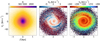 |
Fig. 1. Phase spiral in the solar neighbourhood with Gaia DR3 data. Left: two-dimensional histogram of the vertical projection of phase space (Z–VZ) from the sample of stars with Galactocentric radii of R⊙ ± 0.1 kpc and ϕ = 0 ± 20deg. We used bins of ΔZ = 0.02 kpc and ΔVZ = 1 km s−1. Middle: same projection but colour coded according to median radial velocity VR. Right: same projection but colour-coded according to median azimuthal velocity Vϕ, adjusting the colour bar limits so as to maximise the appearance of the spiral. |
3.2. Detection of the phase spiral
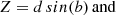
In this section, we describe the method that we used to detect and study the shape of the spiral. It is based on an edge-detector algorithm applied to the counts in the Z–VZ space. We used the implementation in python feature.canny (Canny 1986) from skimage (van der Walt et al. 2014)1. This technique starts by taking the 2D histogram. In most cases starting with a histogram on the logarithm of the number counts worked better (this is our standard option unless stated otherwise). Next, the method reduces the noise using a Gaussian filter kernel with a certain σ (in pixel units). We used a σ that was found empirically to provide good detections. For instance, for the solar neighbourhood and binning defined in the previous subsection, we used σ = 3. For volumes at smaller angular momenta |LZ| explored in the sections below, a larger σ worked better. In particular, we used σ = 4.5 for |LZ|< 1600 km s−1 kpc and σ = 3.5 for |LZ|≥1600 km s−1 kpc. The differences when using different σ are very small for most of cases, and, by construction, they will be within the error bars of the detections (Sect. 4). Next, the algorithm calculates the gradients for each pixel (bin) through the horizontal and vertical Sobel operators, takes the pixels with the maximum gradients, which are always perpendicular to the edges, and further selects the edge bins by hysteresis thresholding. This consists of taking all pixels with gradients above the high threshold (set to 20%) and also, recursively, all the pixels above the low threshold (set to 10%) that are connected to an already taken pixel. All the pixels with gradients below the low threshold are discarded. In practise, the algorithm returns a numerical matrix with values of 1 at the detected edges and 0 otherwise. We note that this detector sometimes has problems in detecting the inner parts of the spiral. However, this is counterbalanced by the simplicity and speed of the algorithm and the good overall detection.
An illustration of the performance of the edge detector for the local phase spiral is shown in Fig. 2. In the top left panel, we superpose the detected edge to the vertical phase-space density. The edge detector perfectly delineates the main spiral and also finds signs of the upper branch in the local phase spiral. There is also a residual detection of an edge at VZ ∼ −70 km s−1 but with a less clear counterpart in the Vϕ-coloured projection. We note that the edge detector obtained from the counts projection approximately follows the spiral in the projection coloured by Vϕ (bottom left panel).
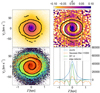 |
Fig. 2. Phase spiral detected by the edge detection. Top left: output of the algorithm applied to the same selection of stars as in Fig. 1, superposed to the counts from which it was computed. We used σ = 3. Bottom left: same but superposed to the projection coloured according to Vϕ. Top right: comparison with the Gaussian filter (colour, see text). Bottom right: comparison with the Gaussian filter and the WT, with the respective values scaled to fit in the same plot, as indicated in the legend, in a one-dimensional case (see text). |
We compared the results from the edge detector with previously used methods, namely the Gaussian filter and the wavelet transform (WT; Antoja et al. 2015 and references therein). Our Gaussian filter is similar to that used by Laporte et al. (2019), but here we use ρ = H2/H4 − 1, where H2 and H4 are the original histogram of counts smoothed by a Gaussian filter (implementation gaussian_filter from scipy, Virtanen et al. 2020) with σG = 2 and σG = 4 (in units of the pixel size, ΔZ and ΔVZ), respectively. For the WT, we use the implementation signal.cwt from scipy with a width of the mother wavelet (Mexican hat) of 3 pixels. The top-right panel of Fig. 2 compares the edge detector with the usual Gaussian filter, while the bottom-right panel compares the three methods for a 1D projection with stars of |VZ|< 3 km s−1. The determinations from the three methods are very similar but the edge detector, by construction, is better at detecting the caustic edge that we are specifically aiming to locate.
3.3. The phase spiral with radius and angular momentum
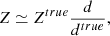
In this section, we explore the spatial evolution of the phase spiral. First, in Fig. 3, we show the phase spiral coloured according to median Vϕ for different Galactocentric radii, from inner (left) to outer radii (right), taking only stars with |ϕ|< 20deg. The phase spiral becomes flatter with radius as already noticed before (e.g., Laporte et al. 2019; Bland-Hawthorn et al. 2019). With DR3, we see that the phase spiral is detected from 6 to 11 kpc, thus extending beyond the previous radial limits. We also see hints of asymmetries reaching 5 and 13 kpc, possibly limited by the selection effects there.
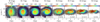 |
Fig. 3. Phase spiral at different Galactocentric radii with Gaia DR3 data. The panels show the vertical projection of phase space (Z–VZ) coloured by median Vϕ. We only use stars with |ϕ|< 20deg. The regions have a total radial width of 1 kpc and their centres are separated by the same amount. We used bins of ΔZ = 0.02 kpc and ΔVZ = 1 km s−1. The colour-map ranges correspond to the percentiles 30 and 70 of the distribution of Vϕ in each volume in order to maximise the appearance of the spiral. We indicate the number of stars in the bottom part of the panels. |
We see a clear additional branching at VZ ∼ 50 km s−1 in the volume at R = 8 kpc, which is already seen in Fig. 1, and now seems to extend slightly towards negative VZ as well. From the animations2 with more continuous sweeping in R, we see that this arch or branch shifts to lower VZ with R, becoming mixed with the upper part of the main phase spiral and turning to an intense red (Vϕ lower than the local median). We also detect what seems to be another turn of the phase spiral or faint arch at VZ ∼ −50 km s−1 at the region of 7 kpc. Curiously, we also see a pattern with a ‘hole’ close to (Z, VZ) = (0, 0) at 10 kpc (already noticed in Gaia DR2, e.g., Laporte et al. 2019).
Separating by LZ instead of current radius yields a clearer spiral signal because binning in LZ groups stars with more similar vertical frequencies (see the Extended Data Figure 4 in A18 and the corresponding explanation), as was clearly demonstrated in Li (2021), Gandhi et al. (2022), and Hunt et al. (2021). However, separating by angular momentum produces different biases, which are well explained by Hunt et al. (2022) for example, the most important being the dominance of eccentric orbits at the extreme angular momentum of the sample.
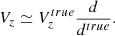
In the top row of Fig. 4 we show phase spiral in counts for different bins of angular momentum. Again we only take stars with |ϕ|< 20deg. In these panels an approximate measure of the guiding radius is given by simply doing Rg = LZ/Vc(R0), assuming a flat circular velocity curve. The black lines show the results of the edge detector (see caption for details). For the last three panels (large angular momentum LZ) we applied the algorithm to the histogram of the counts (instead of the logarithm of the counts as in the other). This detects a better defined spiral for these cases but tends to detect a spiral biased towards inner parts. That is why we only use it for this figure but not when a quantitative comparison between panels needs to be done. In colours we plot the Gaussian filter as in the top right panel of Fig. 2. These panels show well defined phase spirals from Rg ∼ 6 to 11 kpc, and some hints of them beyond these. In the left panels, we see a vertical band empty of stars that is explained by the lack of stars at low |Z| towards the inner Galaxy due to extinction. The flattening of the spiral and their lower number of turns as one moves towards large |LZ| is evident. We note that the double spiral at small angular momentum discovered by Hunt et al. (2022) is not seen here. This could be due to a main phase spiral dominating and masking the double branches here. Alternatively, it could be that, since Hunt et al. (2022) shows the phase spirals for a selection of nearby stars (1 kpc) split by angular momentum, the double spiral is only present for local stars with a small |LZ|, that is when they are observed towards their apocentres. The upper separated branching seen at R ∼ 8 kpc can be seen in the Gaussian filter from Rg ∼ 7.5 to 10 kpc (|LZ| from 1800 to 2400 km s−1kpc). In some cases, for example at |LZ| = 2200 km s−1kpc, further turns at larger |Z| and |VZ| can be seen in the background colours.
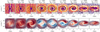 |
Fig. 4. Phase spiral for different angular momenta with Gaia DR3 data. We only use stars with |ϕ|< 20deg. The selections have a total angular momentum width of 200 km s−1 kpc and their centres are separated by the same amount. We used bins of ΔZ = 0.02 kpc and ΔVZ = 1 km s−1. Top: counts projection after Gaussian masking (see text for details). The colour bar is the same as in the top left panel of Fig. 2. We superpose our detected phase spiral via the edge detector method where we used σ = 4.5 for |LZ|< 1600 km s−1 kpc and σ = 3.5 for |LZ|≥1600 km s−1 kpc. We indicate the number of stars in the bottom part of the panels. Bottom: projection coloured by VR with the same colour scale as in the central panel of Fig. 1. |
In the bottom row of Fig. 4, we colour code the vertical phase space according to median VR. A trend of the global VR with LZ is noticeable with redder colours (positive VR) for small |LZ|, bluer (negative VR) for intermediate |LZ|, and again redder for large |LZ|. This is related to the VR − LZ wave detected in Friske & Schönrich (2019; see also Antoja et al. 2022, and the middle panel of the fourth row in Fig. D.1). We also see a quadrupole at the outer parts of these diagrams, which is explained by the tilt of the velocity ellipsoid (Bland-Hawthorn et al. 2019). Aside from these, the phase-spiral segments appear clear and sharp. We note that the correspondence between density phase spiral and coloured by VR is not always direct. For example, the blue VR branch of the phase spiral at LZ = −2200 km s−1 kpc extends to Z = 1.4 kpc while the spiral segment in density continues to curl upwards. In some cases, we see that VR changes its sign along the spiral segments (LZ = −2000 km s−1 kpc).
In Fig. 5, we superpose the phase spirals detected by our algorithm (Sect. 3.2) for different values of LZ as indicated in the legend, supplemented by their corresponding guiding radii Rg assuming a flat circular velocity curve, selecting only stars at the azimuth of the Sun with |ϕ|< 20deg. An animated version of the plot will be made available online3. We see an approximately continuous evolution of the phase spiral with angular momentum. The pitch angle increases as a function of LZ (or R, as already mentioned), as expected. The dark blue curves show some vertical lines related to the selection effects explained above. We note that for the same incremental value in LZ, we do not see the same amount of morphological change; that is, for some angular momenta, the phase spiral changes more abruptly than for others (e.g., from dark to light blue).
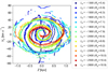 |
Fig. 5. Superposed phase spiral for different angular momenta with Gaia DR3 data. We select stars with ϕ ∈ [ − 20, 20]deg. We use bins of ΔLZ = 200 km s−1 kpc and centres of bins separated by 100 km s−1 kpc, from LZ = −1300 km s−1 kpc (bluer lines) to LZ = −2500 km s−1 kpc (redder lines), as indicted in the legend. In parenthesis, we give an indicative measure of the guiding radius (in kpc), assuming a flat circular velocity curve. |
3.4. Crossing points of the phase spirals with LZ
For the analysis of Sect. 4, we need the Z coordinate of the phase spiral when crossing the VZ = 0 line, which we call Zc. We determined these crossings using our edge-detection algorithm applied to the Z–VZ counts for different selections of angular momentum. We now use samples centred every 50 km s−1 kpc (therefore with more continuity) with a total width of ΔLZ = 100 km s−1 kpc (therefore with some overlap, and smaller than before in order to minimise variations of LZ within a bin). We considered only stars with |ϕ|< 20deg. Figure 6 shows Zc as a function of LZ. In blue we show all the Zc from the edge detector, which show many continuous sequences corresponding to crossings that are well detected across several LZ but also noisy or spurious detections at the extreme LZ, where data are less abundant and distance errors are larger.
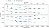 |
Fig. 6. Crossing positions of the phase spiral (Zc). The blue circles and error bars mark the Z coordinate for VZ = 0 of the phase spiral determined from the edge detector for the SH sample. We mark the positions used to infer the impact time with empty black circles. The dashed orange vertical line marks the angular momentum of the Sun. |
Formally, we would assign an error to each Zc of the order of the bin size of the histogram in the Z coordinate to which the edge detector is applied, that is 0.02 kpc. However, we see that using a slightly different σ in the edge detector (from 2 to 5) may (in a few cases) produce differences that are around 0.03 kpc. We therefore take this as our baseline error. We also repeated the measurement of Zc with the BJ distances, computed the difference δZ = |Zc(SH) − Zc(BJ)| between the crossings from SH and BJ (considering the closest points), and arbitrarily assigned an error of MAX(0.03 kpc, δZ) to each Zc from SH. Also, for the final analysis, we only considered Zc with errors smaller than 0.1 kpc (i.e., not considering points in SH that differ from BJ by more than 0.1 kpc). The comparison between the detections with SH and BJ is shown in Fig. B.1. The differences are in general very small, as expected from the small differences in distances at the ranges that we are probing (Appendix B). We also selected only points with |Z|< 1 kpc, since beyond this height the detections are also noisy and in some cases we are not certain whether they really correspond to a crossing of the phase spiral or to some edge of the global distribution. We only took points with LZ ∈ [ − 2600, −1300] km s−1 kpc as the phase spiral is not clear beyond these limits (Fig. 4).
In Fig. 6, the points that we consider valid after all the filters mentioned above are circled in black. At the intermediate LZ part of this figure, corresponding to angular momenta where there are more stars in our sample, more turns are detected (three for Z < 0 compared to two at larger and smaller angular momentum), which is likely due to a combination of the selection effects and true differences in the phase spiral (expected larger pitch angle for larger |LZ|, i.e., less turns). We also see some abrupt jumps such as at LZ ∼ −1600 km s−1 kpc in the lowest turn (Zc ≈ −0.8 kpc). The influence of the selection function on the determinations of Zc is analysed in Appendix D, where we conclude that some of these jumps could be due to slight changes in the dominating population at each LZ. Aside from these jumps, the sequences of Zc show undulations. These are not expected from a simple interpretation of the phase spiral, in which we would see a continuous increase in |Zc| towards the outer parts of the Galaxy (large |LZ|). This is because, in commonly used Galaxy potential models, the gradient of vertical frequencies with vertical amplitude is smaller in the outer parts of the Galaxy (see Extended Data Fig. 4 in A18), leading to a less tightly wound phase spiral. These undulations have important implications in the phase mixing times that we derive from these measurements in Sect. 4.
3.5. The phase spiral with azimuth
Figure 7 shows the azimuthal variations of the phase spiral at fixed angular momentum. We choose LZ ∈ [ − 2100, −1800] km s−1 kpc, because this is the range around the value of LZ with maximum density in our sample. We see fewer changes with ϕ than with LZ but there is a clear gradual change. In some parts of the phase spiral, there is greater variation with azimuth (see e.g., the turn at Z ∼ 0.4) than in other turns (e.g., the turn at −0.5 kpc). In order to quantify these variations, we measure the slope of the crossings Zc as a function of ϕ and find −0.006, −0.004, and 0.002 kpc deg−1 for the crossings at 0.8, 0.3, and −0.6, respectively. The turns at Z ∼ −0.2 and Z ∼ −0.9 remain almost constant with azimuth. A simple phase difference with ϕ would produce the same level of fanning for each turn. Therefore, our observations require an extra deformation (e.g., different level of winding-up at different azimuth, i.e., different phase-spiral pitch angle) and/or strong population differences between positive and negative Z. Finally, we see that the lowest turn of the spiral at VZ ∼ −50 km s−1 is only seen in the azimuths close to the Sun, which is likely due to the increased number of stars in these volumes.
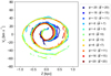 |
Fig. 7. Superposed phase spiral for different azimuths with Gaia DR3 data. We select only stars with LZ ∈ [ − 2100, −1800]. We use bins of Δϕ = 4deg and centres of bins separated by the same amount, from ϕ = −20deg (bluer lines) to ϕ = 20deg (redder lines), as indicted in the legend. In parenthesis, we give the average azimuth of the selection, which can differ by 1deg compared to the centre of the selection in some cases. We used σ = 3.5 for the edge detector. |
4. Inferring the impact time
4.1. Method
In a phase-mixing process, the phase spiral gets more tightly wound with time and we can ‘rewind’ it to infer the onset time of the phase-mixing process, which can then be linked to the time of the perturbation from which it originates. In A18, we used the consecutive turning points of the local phase spiral to constrain the impact time assuming a model of the MW potential from which the vertical frequencies were derived empirically. Here, we repeat the process of A18, but use data of the phase spiral at different angular momenta, helped by the increase in data at different positions across the Galaxy with the new Gaia DR3.
For this analysis, we use the crossings Zc of the phase spiral at VZ = 0 from the previous section (Fig. 6). Stars that have VZ = 0, such as in these crossing points, are currently at their maximum vertical height (above or below the plane): Z = ±Zmax. Therefore, we can estimate the vertical frequencies of these points by interpolating into a grid of frequencies computed as a function of LZ (or Rg) and Zmax. Each pair of consecutive crossings4 (Zc1, Zc2) is then separated by a phase 2π and, thus, we can infer the impact time by their difference in vertical frequency:
 (2)
(2)
Assuming that a single perturbation caused the phase spiral across the disc, this simple analysis should yield the same perturbation time at all LZ and for each pair of crossings. We note that with DR3 we are able to use more pairs of crossings (two in the Z < 0 part of the spiral and one in the Z > 0 part) at an angular momentum closer to that of the Sun, while in A18 we could only use two pairs in total. In A18, we used the crossings detected in the vertical phase space coloured by Vϕ and here we use the crossings from the edge detector on the counts.
To build the grid of frequencies, we used AGAMA (Vasiliev 2019) and simulated more than 8000 orbits at Z ≥ 0 (and use the vertical symmetry of the potential for the Z < 0 part) in the McMillan (2017) potential (McM2017). This is our fiducial potential model. The orbits were integrated for about 50 revolutions. They all started with null VZ (i.e., at the top of their vertical oscillation). The other components of the initial conditions were set as follows: ϕ = 0°, VR = 0 km s−1 (equivalently radial action JR = 0, but see below for orbits with non-null radial action). We then run through Z (from −4 kpc to 4 kpc every 50 pc) and Lz (from 500 km s−1 kpc to 3000 km s−1 kpc every 25 km s−1 kpc), numerically solving the implicit equation
 (3)
(3)
in order to obtain the R, and thus Vϕ = LZ/R, of the corresponding circular orbit. Subsequently, we sample each orbit with 20 000 points5 and measure the vertical frequency with a fast Fourier transformation (Cooley & Tukey 1965) of the signal in Z as a function of time by taking the frequency of the dominant peak (multiple peaks can appear for very eccentric orbits with large vertical-amplitude oscillations). Below we explore other potential models and frequencies for different kinetic temperatures.
4.2. Time results
Interpolating in the above-mentioned grid of frequencies and using Eq. (2), we infer the time of the start of the phase obtained from each pair of crossings Zc. Figure 8 shows the results as a function of LZ (horizontal axis) and Z (colour scale), where for the plot, we used the average (Zc1 + Zc2)/2 of the points of the pair. The time determinations from the Zc that we do not consider valid are marked with small plus symbols (see text in Sect. 3.3; small blue circles in Fig. 6). These appear randomly scattered around the plot (many of these points are outside the vertical range). The circles with error bars are the time determinations from the valid Zc after the considerations of Sect. 3.3. The error bars6 are not symmetric because of the dependency of the frequencies on Z.
 |
Fig. 8. Time of the start of phase mixing as a function of angular momentum. The symbols give the time inferred from Eq. (2) for the different consecutive plus symbols points of the phase spiral and are coloured by height above the plane. The circles with error bars are the points that we consider valid while plus symbols are the remaining cases. An indicative guiding radius corresponding to the circular velocity curve of the McM17 potential is given in the upper horizontal axis. The dashed line marks a linear fit to the data points. |
The valid times in Fig. 8 (error bars) show different coherent sequences. The sequences from small |Zc| (both positive and negative, lighter colours) are distributed around 0.5 Gyr and in many cases are consistent within the errors at a fixed LZ. However, these points show increasing estimated times with |LZ|. In addition, the darker blue points corresponding to the second crossing at Z < 0 are at significantly larger times and also show a tendency to increase with angular momentum. Indeed, a linear fit with LZ to all the valid times (dashed line in Fig. 8) illustrates this global trend.
However, we see several oscillations in the different sequences, some of them corresponding to the oscillations in the Zc (Fig. 6) already mentioned. This is examined further in Appendix D, where we conclude that while some oscillations could be related to changes in the dominating populations, the global trends with LZ and Z might require a different explanation, which we discuss in Sect. 5.
We note that there is certain ambiguity in linking the different Zc into coherent sequences in Fig. 6. For example, it is not clear whether the sequence at Z ≈ −0.25 kpc starting at LZ = −1200 km s−1 kpc−1 continues towards higher or lower Z when reaching LZ = −1600 km s−1 kpc−1. However, the time determinations do not depend on this link to neighbouring points, because they are done independently at each LZ from consecutive crossings in Z. There might be a problem if some crossings are missing but it is unlikely that we have missing crossings in between detected ones: the undetected crossings would be likely located at lower |Z| (the phase spiral is highly undetermined in the central parts of the Z–VZ diagram) and/or at higher |Z| (due to fewer counts). These missing crossings would not bias the estimated times from the intermediate crossings (i.e., would not change from the ones appearing in Fig. 8).
Figure 9 is equivalent to Fig. 8 but shows the time of the start of phase mixing as a function of |Z| (horizontal axis) and LZ (colour scale). A general trend of time increasing with |Z| is observed, as seen in the linear fit (dashed line in Fig. 9). However, this fit would depend on the angular momentum (colours in Fig. 9). Part of these time discrepancies for different Z at fixed LZ could be explained by the fact that the vertical frequency is not perfectly defined for eccentric orbits with large oscillations about the midplane. As we estimate the frequency numerically and take that of the dominant peak, we expect that part of this problem is mitigated.
 |
Fig. 9. Time of the start of phase mixing as a function of height above the plane. The symbols give the time inferred from Eq. (2) for the different consecutive plus symbols points of the phase spiral and are coloured by angular momentum. The circles with error bars are the points that we consider valid while plus symbols are the remaining cases. The dashed line marks a linear fit to the data points. |
Ignoring the trend with Z and LZ (which we discuss in Sect. 5) for now, we obtain an average start of phase mixing time of 0.5 Gyr (0.4 Gyr for the error-weighted average, w = 1/σ2). We find that determinations are within [0.3, 0.9] Gyr 80% of the time. The variations with LZ and Z are larger than the statistical error (error bars). Table 1 (first row) also provides other statistics such as the minimum and maximum values.
Phase-mixing times from the phase spirals.
4.3. Results for different models and data
We examined the dependency of the results on different potential models (Fig. 10), the frequencies for different kinetic temperatures (Fig. 11), and the possible systematic errors on distance (Fig. 12), and looked at the effects of taking the VZ crossings of the spiral with the Z = 0 axis instead of the Zc (see text below, Fig. 13). In all these figures, blue circles show our fiducial case presented above, which consists of using the McM17 potential (non-scaled), SH distances, and JR = 0. The time statistics are given in Table 1, where the last two columns indicate the differences between the times of these new cases and the times from the fiducial case (T0). In most cases, the times are within the error bars of the fiducial case. We find the largest differences when we change the assumed potential model for the MW. In particular, we obtain systematically larger times for Model I (here B08) from Binney & Tremaine (2008; on average 0.09 Gyr larger), and systematically smaller times for the MWpotential2014 (here MW2014) from Bovy (2015) when scaled to fit the values of Vc and R0 used in the data (on average 0.09 Gyr smaller). We also obtain systematically larger times when using not-circular orbits: for example 0.08 Gyr larger times for orbits with radial action JR = 200 km s−1 kpc.
 |
Fig. 10. Time of the start of phase mixing for different potentials. The figure is similar to Fig. 8 but we use frequencies of different potential models of the MW, as indicated in the legend. |
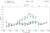 |
Fig. 11. Time of the start of phase mixing for different kinetic temperatures. The figure is similar to Fig. 8 but we use orbits with different radial actions and methods, as indicated in the legend. |
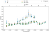 |
Fig. 12. Time of the start of phase mixing for different distances and data. The figure is similar to Fig. 8 but we compare our main results with results using distances from BJ, using distances from SH but adding a distance bias of ±10%, and using a sample of giant stars, as indicated in the legend. |
However, the main trends in the time determinations (in angular momentum and in height) remain the same in all cases. Our conclusions are therefore applicable to all the sets examined. Below we provide details of this analysis; the conclusions are provided in Sect. 5.
We first explored different potential models (Fig. 10), whose circular velocity curves are compared in Fig. F.1. We show the gradient of the vertical frequencies of these models in Fig. F.2. The gradients are slightly different as a function of radius and height but yield only small differences in the time determinations. The orange triangles in Fig. 10 use MW2014. This model returns slightly smaller times at smaller |LZ| and larger times at larger |LZ| but with null average differences when taking all individual time measurements. Purple squares are for B08. With this case, we obtain the largest differences from all the variations explored in this section, that is, systematically larger than our fiducial case and with several points at 2σ. The average differences are of 0.09 Gyr and 80% of the time measurements are within [0.4, 1.] Gyr. We also compared results with these potential models but now scaled to fit the values of Vc and R0 used in the data instead of the original parameters from the respective articles. To do this, we use the built-in scaling mechanism of AGAMA by providing a mass scaling factor (Vc(R0)desired/Vc(R0)default)2 at the time of creating the gravitational potential, which results in the velocities and frequencies being scaled as the square root of this scaling factor. The results for the scaled potentials are shown with the empty symbols in Fig. 10. It is now the MW2014 (scaled) model that gives maximum differences with the fiducial case, yielding smaller times ([0.3, 0.7] Gyr).
Secondly, we examined different orbital conditions (Fig. 11), using frequencies for different kinetic temperatures. In our fiducial case, we use orbits with JR = 0, that is, nearly circular orbits. Here, we increase the eccentricity of the orbits in two different ways and use the corresponding new frequencies. Frequencies for orbits with larger radial actions (JR = 100 & JR = 200 km s−1 kpc, orange squares and green crosses in Fig. 11) yield larger times in general because hotter orbits have smaller differences between frequencies at different heights. Nevertheless, the average time does not change significantly. We also explored frequencies for the most populated part of the distribution function (DF; purple diamonds in Fig. 11). This is done by fixing R and Z and estimating the vertical frequency of the orbit with the highest probability in the DF at that location of space, that is, at Zmax (VZ = 0). With these different frequencies, we also obtain larger times, similar to the JR = 200 case.
Thirdly, we compare our results with those of samples with different distances and different selections of stars (Fig. 12). This is also examined in Appendix C. Using the BJ distances, our results change only very slightly (empty black circles in Fig. 12). This is not surprising given the agreement between both sets of distances for our selected samples. When we consider possible distance biases, we see that if we decrease or increase the distances by 10% (orange and green circles in Fig. B.2), mimicking a correction of overestimated or underestimated distances, respectively, there is an increase or decrease, respectively, in the value of |Zc| by approximately the same amount (Appendix C, Eq. (C.3)), except at the extreme LZ where selection effects might be playing a role. However, as Eq. (2) uses differential frequencies, we see that the times obtained do not change significantly (orange and green triangles in Fig. 12, consistent with the non-biased SH distances within the errors in most cases). We also repeated our analysis using the selection of giant stars from Gaia Collaboration (2023a) obtained from the parameters of the Gaia gspphot pipeline with the same quality filters as for our main sample. The new Zc and derived times are shown in Figs. B.2 and 12 (empty black squares in both figures), respectively. In almost all cases, the new values fall within the error bars of the fiducial case and the trend in angular momentum remains the same. We cannot check whether the times also increase with |Z| because only the inner parts of the spiral are detected due to the small number of stars in this selection (4 901 270).
Finally, we also derive the times from the VZ crossings of the phase spiral at Z = 0, which we name VZ c, in addition to the Z crossings at VZ = 0 (Zc), as we did in A18. More details are given in Appendix E. The location of VZ c with respect to the Zc crossings suggest, among other things, that the assumed potential to infer the frequencies (and therefore the impact times) is not fully correct. We return to this point in our discussion (Sect. 5). As for the obtained times, the overall numbers do not change when considering these new crossings (Fig. 13).
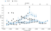 |
Fig. 13. Time of the start of phase mixing for different parts of the phase spiral. The figure is similar to Fig. 8 but we use the fiducial case (blue dots) computed from Zc but also from VZ c (grey squares) to derive the times, as indicated in the legend. |
5. Summary, discussion, and conclusions
We examined the phase spirals in the MW with the new data from Gaia DR3. Our findings can be summarised as follows.
-
We find a clear increase in the Z and VZ ranges in which the phase spiral is detected. Surprisingly, we see the phase spiral extending down to −1.2 kpc, which is well into the realm of the thick disc. This does not necessarily mean that it is made of thick-disc stars but could be made of thin-disc stars that have been largely displaced.
-
We detect phase spiral turns that extend in VZ beyond ±50 km s−1, meaning that the perturbation produced a velocity kick at least of this amount and/or affected stars with these high vertical velocities.
-
An increase in the range of detection of the phase spiral in Galactic radius and azimuth is seen in the new DR3 data. We see clear phase spirals between 6 and 11 kpc in radius and also evident asymmetry, probably indicative of a poorly resolved spiral, down to 5 kpc and up to 13 kpc (Fig. 3).
-
We also see clearer phase spirals in counts and their coloured versions in radial and azimuthal velocities.
-
We detect a secondary branch of the phase spiral at large positive VZ in the counts projection and in the phase spiral painted by Vϕ. This is observed in the local phase spiral (see also A18 and Laporte et al. 2019) but also at angular momenta between 1800 and 2400 km s−1kpc. This branch seems to merge with the well-defined main phase spiral moving towards the outer Galaxy. A somewhat similar branching is seen in the simulations by Hunt et al. (2021; their Fig. 5). This secondary branch might be caused by the complexity of the phase-mixing process (e.g. different groups of actions, stemming from non-uniform initial conditions, or with strong dependence on the position of the disc) or different perturbations.
-
The phase spiral has different morphology when splitting by angular momentum, including the expected flattening with Z at larger |LZ| (also seen in DR2, e.g., Laporte et al. 2019; Bland-Hawthorn et al. 2019) but also trends departing from this expected flattening in a usual MW gravitational potential. While part of these trends could be due to selection effects (Appendix D), a more straightforward explanation might be our overly simplistic modelling of the phenomena involved (see below).
-
We see differences in the spiral in counts and coloured by VR at certain angular momentum. As seen in the simulations in Bland-Hawthorn & Tepper-García (2021) for an impact with a galactic satellite, the vertical projection of phase space coloured by VR could be a result of the combination of: (1) the density wave induced after a perturbation (mostly a two-armed spiral density structure in the impulsive and distant impact conditions; Toomre & Toomre 1972; Struck et al. 2011) that is linked to a LZ–VR wave (Antoja et al. 2022), and (2) the vertical waves induced after the same perturbation. However, the exact way in which the planar and vertical disturbances are coupled is not yet well understood. Joining simple modelling of satellite perturbations such as those in Gandhi et al. (2022; vertical) and Antoja et al. (2022; planar) could help in this respect. Exploring more complex models with sufficient resolution, such as those in Hunt et al. (2022), is also necessary.
-
We detect mild changes of the phase spiral at different azimuth. Their Z coordinates at VZ = 0 can differ by up to −0.006 kpc deg−1 but these changes are not uniform (i.e., they depend on the turn of the phase spiral).
Finally, we estimated the phase-mixing times from the phase spiral for the first time using data at different angular momenta. Our findings from this part of the analysis can be summarised as follows.
-
There is a large amount of variation in the times derived from measurements of the phase spiral at different heights (different turns) and at different angular momenta: we see an increase in time with |LZ| and especially with |Z|. The time differences can be of 0.7 Gyr using a single phase spiral at the angular momentum close to that of the Sun but different turns of the phase spiral (i.e., different Z) and of 0.4 Gyr considering different angular momenta.
-
The average time is of 0.5 Gyr. For 80% of our determinations, we find times in the range of 0.3–0.9 Gyr.
-
We find slightly larger times when using the B08 model (0.4–1 Gyr), systematically larger times for hotter orbits (0.4–1. Gyr), and smaller times for a rescaled version of MW2014 (0.3–0.7 Gyr).
-
The values obtained are very similar to the ones given in A18, which were 0.3–0.9 Gyr and are consistent in their upper limits with the determinations from the frequency of the LZ–VR wave from Antoja et al. (2022). As in our original work, A18, these times are consistent with a previous pericentre passage of Sagittarius.
-
The mentioned trends with angular momentum and height are robust to using frequencies for hotter orbits, different potential models, different distance determinations, and possible (small) distance biases.
We note that our modelling of the phase spiral could be oversimplistic. For example, we only consider the crossings of the phase spiral with the Z = 0 and VZ = 0 axis but it would be better to use the continuity of the entire phase spiral. This would be more in line with the work of Widmark et al. (2021). Recently, we found out that studies carried out simultaneously to ours (Frankel et al. 2023; Darragh-Ford et al. 2023) used action-angle variables in an assumed potential to unwind the spiral into a ‘straight’ line for the time fit. While our method does not use the full information of the phase spiral at the same time, it confers a slight advantage in that it does not require the assumption of a potential until the final steps, making it easier to use in a combined fit of the phase-mixing time and potential. In any case, these studies also find different time determinations at different angular momenta (between 0.2 and 0.6 Gyr in Frankel et al. 2023; 0.3 and 1 Gyr Darragh-Ford et al. 2023) and with different radius and azimuth (between 0.3 and 0.8 Gyr in Widmark et al. 2022b), which is similar to our results.
These differences in the obtained times for different angular momenta and heights are not expected in the simplest interpretation of the phase spiral coming from a phase-mixing process. Below we discuss different explanations.
It could be that we are seeing differences in the time of response to the perturbation of different disc regions. However, for the case of the Sagittarius impact studied by Gandhi et al. (2022), the authors found differences in the onset of the perturbation effects at different radii of the order of 100 Myr, which is smaller than what we measure. In addition, they do not see a clear trend with guiding radius. Widmark et al. (2022a) tested their machinery of determining the potential from the phase spiral shape on the N-body simulation from Hunt et al. (2021) and found time differences in small ranges of R of the order of 100–200 Myr. In test-particle simulations, Darragh-Ford et al. (2023) find slightly larger (≈200 Myr) time variations with position (guiding centre coordinates). In addition, the time differences with Z at a fixed angular momentum would be hard to explain with this hypothesis alone, although as discussed above, our method could be affected by bias for large Z. The spatial and temporal propagation of different bending waves remains poorly studied and we plan to examine this with various models in the future.
Another explanation is that there is a mismatch between the vertical and radial dependence of the potential in the models (that we used to compute the vertical frequencies) and in the real MW. We also find possible evidence for this mismatch by considering and comparing the coordinates of the phase spiral when crossing the Z = 0 and the VZ axis (Appendix E). One could infer the potential that could make these trends disappear. For example, the linear trend seen with LZ (dashed line in Fig. 8) could be used to ‘correct’ the potential (the gradient in frequencies) in order to obtain similar times. This is not trivial because of the degeneracy and the possible self-gravity effects.
Indeed, the time variations could also be evidence for self-gravity acting differently in different parts of the disc. Self-gravity tends to amplify the phase-mixing times (Darling & Widrow 2019) and in particular could be of less importance in the outer parts of the disc (e.g., Shen & Sellwood 2006). This could mean that the times that we obtain in the outer parts, that is the larger times, are closer to the true perturbation time. However, the radial behaviour of different kinds of bending waves that originate from different perturbations might be different (e.g., bending waves associated to the bar or due to external torques from galactic satellites or even from a misaligned halo) and this possibility has not been thoroughly studied. Recently, Darragh-Ford et al. (2023) found large offsets between the interaction time and the recovered time in their N-Body simulation using their action-angle modelling, which they attribute to self-gravity or the effects of the associated halo wake.
Finally, our finding could be related to other aspects of the disc dynamics and how they interact with each other. By this, we mean the effects of the bar, the spiral arms, the warp, and different bending and breathing modes, which could have acted or be acting in addition to the vertical perturbation causing the phase spiral. For instance, Widmark et al. (2022c) recently showed that some features of the vertical density and velocity seem related to the local spiral arm, while theoretical studies have also led to the identification of vertical velocity effects in spiral arm models (e.g., Faure et al. 2014; Kumar et al. 2022). In addition, if the disc mid-plane oscillates because of one of these additional distinct phenomena, the Z–VZ centroid of the phase spiral will oscillate and affect the time determinations (Appendix E).
In conclusion, we are now able to see a higher level of complexity in the morphology of the vertical projection, as well as unexpected trends, possibly indicating different perturbations (perhaps from different agents or different times), as already pointed out by Hunt et al. (2022) – following the discovery of the double phase spirals –, and/or complex phase mixing processes. The variations that we see in our derived phase-mixing times with vertical position and angular momentum likely indicate inadequate modelling due to uncertainties in the potential model for the Galaxy; our neglect of self-gravity; the existence and interaction of multiple perturbations, or a combination of these. Although the new Gaia DR3 data definitively bring us a clearer picture of the MW phase spirals, there is still much to be understood and modelled.
We tested the sensitivity of the measured frequency to both the number of samples used and the number of revolutions, finding a negligible dependence on the former (as long as there are more than a few hundred points) and an asymptotic behaviour as a function of the latter. For 50 revolutions, the error on the measured frequency tends to be of the order of less than 1%.
To compute the upper (lower) limit in each derived time, we used the limits of the errors of Zc that minimise (maximise) the frequency difference. That is, for pairs of crossings with Z > 0, we considered the lower limit of the smaller Zc and the upper limit of the larger Zc to obtain the lower limit on the time (maximum vertical-frequency difference). Conversely, the upper limit on time is obtained by combining the upper limit of the smaller Zc and the lower limit of the larger Zc.
The area covered by a constant angular step increases along the spiral, as the distance from the centre grows, which causes the consequent drop in density we try to counteract by drawing the angles of the particles along the spiral from a Beta probability distribution function with a = 2 and b = 5. In other words, the angles along the spiral are not drawn uniformly.
Acknowledgments
Project supported by a 2021 Leonardo Grant for Researchers and Cultural Creators, BBVA Foundation. The BBVA Foundation accepts no responsibility for the opinions, statements and contents included in the project and/or the results thereof, which are entirely the responsibility of the authors. This work was (partially) supported by the Spanish MICIN/AEI/10.13039/501100011033 and by “ERDF A way of making Europe” by the “European Union” through grant PID2021-125451NA-I00, and the Institute of Cosmos Sciences University of Barcelona (ICCUB, Unidad de Excelencia ‘María de Maeztu’) through grant CEX2019-000918-M. TA acknowledges the grant RYC2018-025968-I funded by MCIN/AEI/10.13039/501100011033 and by “ESF Investing in your future”. BGC acknowledges financial support from the Spanish Ministry of Economy and Competitiveness (MINECO) under grant number RTI2018-096188-B-I00 and IPARCOS Institute for the grant “Ayudas de doctorado IPARCOS-UCM/2022”. MB received funding from the University of Barcelona’s official doctoral program for the development of a R+D+i project under the PREDOCS-UB grant. CL acknowledges funding from the European Research Council (ERC) under the European Union’s Horizon 2020 research and innovation programme (grant agreement No. 852839). This work has made use of data from the European Space Agency (ESA) mission Gaia (https://www.cosmos.esa.int/gaia), processed by the Gaia Data Processing and Analysis Consortium (DPAC, https://www.cosmos.esa.int/web/gaia/dpac/consortium). Funding for the DPAC has been provided by national institutions, in particular the institutions participating in the Gaia Multilateral Agreement.
References
- Anders, F., Khalatyan, A., Queiroz, A. B. A., et al. 2022, A&A, 658, A91 [NASA ADS] [CrossRef] [EDP Sciences] [Google Scholar]
- Antoja, T., Mateu, C., Aguilar, L., et al. 2015, MNRAS, 453, 541 [NASA ADS] [CrossRef] [Google Scholar]
- Antoja, T., Helmi, A., Romero-Gómez, M., et al. 2018, Nature, 561, 360 [Google Scholar]
- Antoja, T., Ramos, P., López-Guitart, F., et al. 2022, A&A, 668, A61 [NASA ADS] [CrossRef] [EDP Sciences] [Google Scholar]
- Bailer-Jones, C. A. L. 2015, PASP, 127, 994 [Google Scholar]
- Bailer-Jones, C. A. L., Rybizki, J., Fouesneau, M., Demleitner, M., & Andrae, R. 2021, AJ, 161, 147 [Google Scholar]
- Banik, U., Weinberg, M. D., & van den Bosch, F. C. 2022, ApJ, 935, 135 [NASA ADS] [CrossRef] [Google Scholar]
- Bennett, M., & Bovy, J. 2019, MNRAS, 482, 1417 [NASA ADS] [CrossRef] [Google Scholar]
- Bennett, M., Bovy, J., & Hunt, J. A. S. 2022, ApJ, 927, 131 [NASA ADS] [CrossRef] [Google Scholar]
- Binney, J., & Schönrich, R. 2018, MNRAS, 481, 1501 [Google Scholar]
- Binney, J., & Tremaine, S. 2008, Galactic Dynamics, 2nd edn. (Princeton: Princeton University Press) [Google Scholar]
- Bland-Hawthorn, J., & Gerhard, O. 2016, ARA&A, 54, 529 [Google Scholar]
- Bland-Hawthorn, J., Sharma, S., Tepper-Garcia, T., et al. 2019, MNRAS, 486, 1167 [NASA ADS] [CrossRef] [Google Scholar]
- Bland-Hawthorn, J., & Tepper-García, T. 2021, MNRAS, 504, 3168 [CrossRef] [Google Scholar]
- Blomme, R., Frémat, Y., Sartoretti, P., et al. 2023, A&A, in press, https://doi.org/10.1051/0004-6361/202243685 [Google Scholar]
- Bovy, J. 2015, ApJS, 216, 29 [NASA ADS] [CrossRef] [Google Scholar]
- Canny, J. 1986, Pattern Analysis and Machine Intelligence, IEEE Transactions on PAMI-8, 679 [CrossRef] [Google Scholar]
- Chequers, M. H., Widrow, L. M., & Darling, K. 2018, MNRAS, 480, 4244 [CrossRef] [Google Scholar]
- Chrobáková, Ž., López-Corredoira, M., Sylos Labini, F., Wang, H. F., & Nagy, R. 2020, A&A, 642, A95 [NASA ADS] [CrossRef] [EDP Sciences] [Google Scholar]
- Cooley, J. W., & Tukey, J. W. 1965, Math. Comp., 19, 297 [CrossRef] [MathSciNet] [Google Scholar]
- Darling, K., & Widrow, L. M. 2019, MNRAS, 484, 1050 [CrossRef] [Google Scholar]
- Darragh-Ford, E., Hunt, J. A. S., Price-Whelan, A. M., & Johnston, K. V. 2023, ArXiv e-prints [arXiv:2302.09086] [Google Scholar]
- Faure, C., Siebert, A., & Famaey, B. 2014, MNRAS, 440, 2564 [CrossRef] [Google Scholar]
- Frankel, N., Bovy, J., Tremaine, S., & Hogg, D. W. 2023, MNRAS, 521, 5917 [NASA ADS] [CrossRef] [Google Scholar]
- Friske, J. K. S., & Schönrich, R. 2019, MNRAS, 490, 5414 [Google Scholar]
- Gaia Collaboration (Prusti, T., et al.) 2016, A&A, 595, A1 [NASA ADS] [CrossRef] [EDP Sciences] [Google Scholar]
- Gaia Collaboration (Brown, A. G. A., et al.) 2018, A&A, 616, A1 [NASA ADS] [CrossRef] [EDP Sciences] [Google Scholar]
- Gaia Collaboration (Drimmel, R., et al.) 2023a, A&A, in press, https://doi.org/10.1051/0004-6361/202243797 [Google Scholar]
- Gaia Collaboration (Recio-Blanco, A., et al.) 2023b, A&A, in press, https://doi.org/10.1051/0004-6361/202243511 [Google Scholar]
- Gaia Collaboration (Vallenari, A., et al.) 2023c, A&A, in press, https://doi.org/10.1051/0004-6361/202243940 [Google Scholar]
- Gandhi, S. S., Johnston, K. V., Hunt, J. A. S., et al. 2022, ApJ, 928, 80 [NASA ADS] [CrossRef] [Google Scholar]
- García-Conde, B., Roca-Fàbrega, S., Antoja, T., Ramos, P., & Valenzuela, O. 2022, MNRAS, 510, 154 [Google Scholar]
- Grand, R. J. J., Pakmor, R., Fragkoudi, F., et al. 2022, MNRAS, submitted [arXiv:2211.08437] [Google Scholar]
- Gravity Collaboration (Abuter, R., et al.) 2022, A&A, 657, L12 [NASA ADS] [CrossRef] [Google Scholar]
- Haines, T., D’Onghia, E., Famaey, B., Laporte, C., & Hernquist, L. 2019, ApJ, 879, L15 [Google Scholar]
- Hunt, J. A. S., Stelea, I. A., Johnston, K. V., et al. 2021, MNRAS, 508, 1459 [NASA ADS] [CrossRef] [Google Scholar]
- Hunt, J. A. S., Price-Whelan, A. M., Johnston, K. V., & Darragh-Ford, E. 2022, MNRAS, 516, L7 [NASA ADS] [CrossRef] [Google Scholar]
- Katz, D., Sartoretti, P., Guerrier, A., et al. 2023, A&A, in press, https://doi.org/10.1051/0004-6361/202244220 [Google Scholar]
- Khoperskov, S., Di Matteo, P., Gerhard, O., et al. 2019, A&A, 622, L6 [NASA ADS] [CrossRef] [EDP Sciences] [Google Scholar]
- Kumar, A., Ghosh, S., Kataria, S. K., Das, M., & Debattista, V. P. 2022, MNRAS, 516, 1114 [NASA ADS] [CrossRef] [Google Scholar]
- Laporte, C. F. P., Johnston, K. V., Gómez, F. A., Garavito-Camargo, N., & Besla, G. 2018, MNRAS, 481, 286 [Google Scholar]
- Laporte, C. F. P., Minchev, I., Johnston, K. V., & Gómez, F. A. 2019, MNRAS, 485, 3134 [Google Scholar]
- Li, Z.-Y. 2021, ApJ, 911, 107 [NASA ADS] [CrossRef] [Google Scholar]
- Li, Z.-Y., & Shen, J. 2020, ApJ, 890, 85 [NASA ADS] [CrossRef] [Google Scholar]
- Luri, X., Brown, A. G. A., Sarro, L. M., et al. 2018, A&A, 616, A9 [NASA ADS] [CrossRef] [EDP Sciences] [Google Scholar]
- McMillan, P. J. 2017, MNRAS, 465, 76 [NASA ADS] [CrossRef] [Google Scholar]
- Mor, R., Robin, A. C., Figueras, F., Roca-Fàbrega, S., & Luri, X. 2019, A&A, 624, L1 [NASA ADS] [CrossRef] [EDP Sciences] [Google Scholar]
- Purcell, C. W., Bullock, J. S., Tollerud, E. J., Rocha, M., & Chakrabarti, S. 2011, Nature, 477, 301 [Google Scholar]
- Reid, M. J., & Brunthaler, A. 2020, ApJ, 892, 39 [Google Scholar]
- Ruiz-Lara, T., Gallart, C., Bernard, E. J., & Cassisi, S. 2020, Nat. Astron., 4, 965 [NASA ADS] [CrossRef] [Google Scholar]
- Rybizki, J., Green, G. M., Rix, H.-W., et al. 2022, MNRAS, 510, 2597 [NASA ADS] [CrossRef] [Google Scholar]
- Shen, J., & Sellwood, J. A. 2006, MNRAS, 370, 2 [NASA ADS] [CrossRef] [Google Scholar]
- Struck, C., Dobbs, C. L., & Hwang, J.-S. 2011, MNRAS, 414, 2498 [NASA ADS] [CrossRef] [Google Scholar]
- Tian, H.-J., Liu, C., Wu, Y., Xiang, M.-S., & Zhang, Y. 2018, ApJ, 865, L19 [NASA ADS] [CrossRef] [Google Scholar]
- Toomre, A., & Toomre, J. 1972, ApJ, 178, 623 [Google Scholar]
- Tremaine, S., Frankel, N., & Bovy, J. 2023, MNRAS, 521, 114 [NASA ADS] [CrossRef] [Google Scholar]
- van der Walt, S., Schönberger, J. L., Nunez-Iglesias, J., et al. 2014, PeerJ, 2, e453 [Google Scholar]
- Vasiliev, E. 2019, MNRAS, 482, 1525 [Google Scholar]
- Virtanen, P., Gommers, R., Oliphant, T. E., et al. 2020, Nat. Methods, 17, 261 [Google Scholar]
- Wang, C., Huang, Y., Yuan, H. B., et al. 2019, ApJ, 877, L7 [NASA ADS] [CrossRef] [Google Scholar]
- Widmark, A., de Salas, P. F., & Monari, G. 2021, A&A, 646, A67 [NASA ADS] [CrossRef] [EDP Sciences] [Google Scholar]
- Widmark, A., Hunt, J. A. S., Laporte, C. F. P., & Monari, G. 2022a, A&A, 663, A16 [NASA ADS] [CrossRef] [EDP Sciences] [Google Scholar]
- Widmark, A., Laporte, C. F. P., & Monari, G. 2022b, A&A, 663, A15 [NASA ADS] [CrossRef] [EDP Sciences] [Google Scholar]
- Widmark, A., Widrow, L. M., & Naik, A. 2022c, A&A, 668, A95 [NASA ADS] [CrossRef] [EDP Sciences] [Google Scholar]
- Widrow, L. M., Gardner, S., Yanny, B., Dodelson, S., & Chen, H.-Y. 2012, ApJ, 750, L41 [Google Scholar]
- Williams, M. E. K., Steinmetz, M., Binney, J., et al. 2013, MNRAS, 436, 101 [Google Scholar]
- Younger, J. D., Besla, G., Cox, T. J., et al. 2008, ApJ, 676, L21 [Google Scholar]
Appendix A: Queries used to select samples
In this Appendix, we show a few examples of queries to the Gaia Archive https://gea.esac.esa.int/archive/ to retrieve the data:
Listing 1. This query is used to retrieve stars with radial velocity with additional selection in temperature and RUWE (see main text) for our basic sample.
SELECT gaia.source_id,gaia.ra,gaia.dec,
gaia.parallax,gaia.pmra,gaia.pmdec,
gaia.radial_velocity,gaia.parallax_error,
gaia.phot_g_mean_mag,gaia.bp_rp,
gaia.grvs_mag,gaia.rv_template_teff
FROM gaiadr3.gaia_source AS gaia
WHERE gaia.radial_velocity is not null   AND gaia.ruwe
     < 1.4 AND gaia.rv_template_teff<8500
Listing 2. This query is used to retrieve the fidelity flag (see main text) that is later merged by source_id with the data from query 1 for additional selection.
SELECT Rybizki.source_id, Rybizki.fidelity_v2
FROM external.gaiaedr3_spurious AS Rybizki
JOIN gaiadr3.gaia_source AS gaia  ON gaia.source_id =
    Rybizki.source_id
WHERE gaia.radial_velocity is not null
Listing 3. This query is used to retrieve the BJ distance (see main text) that is later merged by source_id with the data from query 1.
SELECT CBJ.source_id, CBJ.r_med_photogeo
FROM external.gaiaedr3_distance AS CBJ
JOIN gaiadr3.gaia_source AS gaia  ON gaia.source_id =
    CBJ.source_id
WHERE gaia.radial_velocity is not null
Listing 4. This query is used to retrieve the source_id of giants stars that is later merged by source_id with the data from query 1.
SELECT g.source_id
FROM gaiadr3.gaia_source AS g
WHERE (g.teff_gspphot<5500 and g.teff_gspphot>3000)
and (g.logg_gspphot<3.) and (g.radial_velocity is not
     null)
Appendix B: Different distances
Here we compare the SH and the BJ distances of the 25 385 209 stars that remain after the cuts specified in Sect. 2. This is shown in Fig. B.1. On average, there is a negligible bias between distances. For example, the relative differences are of 0.8% at around 1.5 kpc and of -0.9% at 4 kpc, that is smaller than 1% for the distances we are dealing with. For 80% of the stars, the differences are smaller than 11% up to 4 kpc. Indeed, when we calculate our Zc using the different distance sets, our values change only very slightly (Fig. B.2) and, consequently, our derived times do not change significantly either (Fig. 12).
 |
Fig. B.1. Comparison between sets of distances. Relative differences between distances from SH (Anders et al. 2022) and BJ distances (Bailer-Jones et al. 2021) as a function of SH distances for the stars in our sample for which these two distances are available. The black line shows the median of the distribution, while the blue and red lower and upper lines show the 10 and 90 percentiles (i.e. they enclose 80% of stars). |
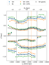 |
Fig. B.2. Crossing positions of the phase spiral for different distances. The blue circles and error bars mark the Z coordinate for VZ = 0 (Zc) of the phase spiral determined from the edge detector for the SH sample. The other symbols indicate the crossings for the BJ distances, for distance biases of 10%, and for a selection of giant stars. |
Appendix C: Effect of distance bias on the parameters of the phase spiral
Given that Z and Vz can be written as
 (C.1)
(C.1)
 (C.2)
(C.2)
we can make some approximate calculations to understand how the distances affect the shape of the phase space spiral.
Assuming that the effect of the distance bias only manifests at a certain distance, and that the range in Galactic latitude for disc stars shrinks with this distance, we can neglect the contribution of the line-of-sight velocity to Vz without loss of generality. We can further assume that the errors in the sky position are negligible, and that proper-motion errors are perfectly Gaussian. If we do so, it is trivial to prove that, on average,
 (C.3)
(C.3)
and, similarly,
 (C.4)
(C.4)
This result implies that both coordinates will suffer from a bias in the distance in a similar manner, at any position in the disc. For instance, if the distances are underestimated by 10%, the phase space spiral will shrink by the same amount, thus keeping the proportions. However, we note that even if proportions are kept, the pitch angle will change and become larger if the spiral shrinks, and smaller if the spiral grows.
In general, we know that the bias increases with distance for most distance estimators based fully, or even partially, on the parallax. Therefore, the amount by which the spiral shrinks or grows will change as a function of Z for a certain X and Y, as the heliocentric distance will increase with Z. Therefore, the deformation will not be as simple as a scaling of the original one.
Moreover, the process of estimating a distance from a parallax for one star usually leads to a probability distribution of distances that is not symmetric. Therefore, rather than having a simple bias, normally the mode of the resulting distance probability distribution is smaller than the true distance (which should coincide with the median), causing in turn a long tail towards large distances (Luri et al. 2018). This further complicates any attempt to predict the appearance of the phase spiral.
To test these deductions, first we generate particles along a perfect Archimedean spiral in a manner such that the number of particles increases with the distance from the centre, which we do simply for visualisation purposes7. Once we have this true spiral, we place it at a certain heliocentric distance of our choice (this is the distance of the particles at Z = 0), and then calculate the true distance of all the particles in it by inverting Eqs. C.1 and C.2. We then draw a parallax for each particle from a normal distribution centred at its true parallax (inverse of its true distance), with an error set to a certain parallax over error.
The left column of Fig. C.1 shows the effects of assuming a fixed parallax over error of 5 for all particles on a spiral that is located at 4 kpc from the Sun. The different rows correspond to different distances estimates: inverting the parallax or using the Bailer-Jones (2015) exponentially decreasing volume prior with different parameters. As we can see, the peak of the density is displaced inwards as expected (see above), with a long tail outwards accompanying it that blurs the signal. The right column of Fig. C.1 is similar to the left column, but now we have sampled the parallax over error randomly in the range from 1 to 10. This results in a less biased and slightly more blurred spiral. The differences between rows (distance estimates) here is almost unnoticeable, although using the median (bottom-right panel) instead of the mode of the posterior (second and third rows on the right) seems to provide less biased results. However, in general, we will have a mixture of populations that depends on the location with respect to the Sun of the bin we are sampling, that is on the magnitude and colour distribution of the stars in that subsample and their heliocentric distances. Therefore, even if we cannot quantify the exact deformation of the spiral, it seems reasonable to expect it to shrink.
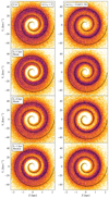 |
Fig. C.1. Effects of the distance bias on a perfect Archimedean spiral. For all panels, the centre of the spiral is at 4 kpc from the Sun, and the black curve is the true spiral. Left column: Mock particles sampled with a constant parallax over error of 5. Right column: Same but the parallax over error is sampled uniformly from 1 to 10. Rows correspond to different distance estimates, from top to bottom: parallax inversion; Bayesian estimate with L = 1 kpc and taking the mode of the posterior; same as above but with L = 4 kpc; Bayesian estimate with L = 1 kpc but taking the median of the posterior. |
As a second test, we now recompute the phase-space coordinates of the full sample after enlarging and decreasing their distances by 10%. These two new dummy samples help us, to begin with, to confirm that the approximations presented in Eqs. C.3 and C.4 are valid in general. More importantly, with the new sample, we can redo all calculations of our analysis. First in Fig. B.2, we show the Zc of the phase spiral when distances are decreased by 10% (orange circles) and increased by 10% (green) which can be compared to the unscaled SH distances (blue circles). In general, we find that the bias mostly reproduces our expectations, that is the Zc are scaled by ±10%. Some points differ from these expectations, which might be due to selection effects. Fig. 12 shows the recomputed phase mixing times for these new Zc and we find that, in most cases, they fall within the errors of the fiducial case (in 80% of the cases). More details are given in the main text. We note that although the biased Zc do not fall within the errors of the initial (unbiased) Zc, this is not the case for the time determinations. This is because, to compute a time and its error bar, we use two consecutive Zc and combine the different upper and lower limits of these two Zc to obtain the minimum and maximum frequency differences that give rise to the maximum and minimum times, respectively.
Appendix D: Selection effects
In this Appendix, we examine the possible effects of the selection function of our samples in the determined Zc and phase-mixing times. The Gaia selection function is definitively a complicated matter. A possible worry for our work is that the characteristics of our sample, which certainly change with R and Z, bias our results. At different parts of the phase spiral and at different angular momenta, the dominating population might change. For example, the proportion of thick-disc over thin-disc stars or the average age can vary with radius. In particular, the average radial action of stars might change. We used actions computed in Gaia Collaboration (2023b) to check that mean values of the radial action in the LZ and Z ranges explored here go from about 20 to 80 km s−1kpc (the 75 percentile can reach 120 km s−1kpc). However, here we find that changing from JR = 0 to 200 km s−1kpc gives time differences mostly in the range of [0.04, 0.16] (Table 1), which is smaller than the systematic differences seen with angular momentum and height (Fig. 8). The trends of the derived times with angular momentum (and height) are hard to explain with only selection effects.
We nevertheless explore the mean value of different variables as a function of LZ for the sample of stars with |ϕ|< 20deg that is used in most of our analysis. This is shown in Figure D.1. Most of the quantities show a similar pattern (peak or valley at the Sun’s angular momentum, orange vertical dashed line) that is explained by having increasing distance for values of the |LZ| departing from that of the Sun (right panel in the fifth row). It is not straightforward to translate this trend into a trend in LZ (or in Z) because it is the difference between frequencies that enters in the calculation, but the peak and valley trends make the time increase with |LZ| hard to explain. By contrast, the hypotheses given in the discussion in the main text (incorrectness of the potential models, neglect of self-gravity, etc.) are easier to explain and are somewhat expected causes.
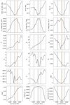 |
Fig. D.1. Investigation of some selection function effects. Mean values of different variables as a function of angular momentum LZ. The dashed vertical lines indicate some positions where we see jumps in the shape of the phase spiral and/or the determined phase mixing times. The orange dashed line is the angular momentum of the Sun. |
In all panels of Figure D.1, we use vertical black dashed lines to mark some positions of discontinuity in the Zc (LZ = −1575 and -2275 km s−1kpc, also marked in Fig. B.2) and in the time determinations (LZ = −1975 km s−1kpc). Some of the lines could be correlated with jumps for example in the average magnitude of stars (two first panels of the first row, but with very small difference in magnitude) or with slight changes in the trends of colour (right panel in the first row). We also see some correlation with the known wave in VR (middle panel in the fourth row). At this point, we cannot therefore discard that the jumps are selection effects or conclude that they are real physical effects.
Appendix E: Additional tests
Here, we examine the consecutive VZ crossings of the phase spiral at Z = 0, which we name VZ c. To determine the VZ c we use the same method as for Zc based on the edge detector. We then find the maximum Z corresponding to an orbit with that maximum VZ under the fiducial potential. We do this using the same orbital integrations carried out to determine the vertical frequency, for which, at each LZ, we have a pair of maximum Z and VZ. This can be thought of as obtaining a new set of Zc that can be compared to the previous ones. We can examine whether these new Zc sequences run through the middle of the previous Zc sequences, as expected from the most simple interpretation of the phase spiral. The results of this test (Fig. E.1) show that this is not fulfilled when we assume our fiducial potential, as we see some sequences overlapping. Our understanding is that this might have several implications, with the simplest one being that our assumed potential is incorrect. Other interpretations could be an underlying complex bending wave, time dependence of the global potential, or the existence of multiple interfering phase spirals.
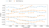 |
Fig. E.1. Crossing positions of the phase spiral in the VZ = 0 and Z = 0 axis. The blue circles mark the Z coordinate of the phase spiral at VZ = 0 (Zc) determined from the edge detector for the SH sample. The orange squares indicate the Zc corresponding to the crossings VZ c at the Z = 0 axis (see text). |
We run a second test in which we compare the Zc for either Z > 0 or Z < 0. Again in the most simple interpretation of the phase spiral, we should expect that |Zc| sequences at Z < 0 (i.e. when we consider the absolute value of Zc from crossings of the phase spiral at Z < 0) run approximately through the middle of the Zc sequences at Z > 0. This is studied in Fig. E.2 and we see that the red sequences (from Z < 0) are roughly but not exactly in the middle of the blue sequences (from Z > 0). For instance, there are crossings of red and blue sequences at certain positions, where we already identified jumps or undulations. This could be evidence of the existence of a bending wave in the disc that is superimposed over the phase spiral patterns. However, if this is the case, it does not appear as a simple wave that can be easily subtracted. Also, in the case of having a bending wave, the reference system, the potential, and the vertical frequencies would be somehow ill-defined concepts, and thus our modelling would not be appropriate. On the other hand, this could be evidence of more complex phase mixing, as the rest of our study also suggests.
 |
Fig. E.2. Crossing positions of the phase spiral for Z > 0 and Z < 0. The blue and red circles mark the |Z| coordinate of the phase spiral at VZ = 0 (Zc) for positive and negative Z, respectively. |
Appendix F: Additional material
Here we present the different gravitational potential models for the MW used in our study (Fig. F.1) and their respective vertical gradients in the vertical frequencies (Fig. F.2).
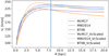 |
Fig. F.1. Circular velocity curves of the different potentials used. |
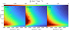 |
Fig. F.2. Vertical gradient of the vertical frequencies for the different potentials used. |
All Tables
All Figures
|
Fig. 1. Phase spiral in the solar neighbourhood with Gaia DR3 data. Left: two-dimensional histogram of the vertical projection of phase space (Z–VZ) from the sample of stars with Galactocentric radii of R⊙ ± 0.1 kpc and ϕ = 0 ± 20deg. We used bins of ΔZ = 0.02 kpc and ΔVZ = 1 km s−1. Middle: same projection but colour coded according to median radial velocity VR. Right: same projection but colour-coded according to median azimuthal velocity Vϕ, adjusting the colour bar limits so as to maximise the appearance of the spiral. |
| In the text | |
|
Fig. 2. Phase spiral detected by the edge detection. Top left: output of the algorithm applied to the same selection of stars as in Fig. 1, superposed to the counts from which it was computed. We used σ = 3. Bottom left: same but superposed to the projection coloured according to Vϕ. Top right: comparison with the Gaussian filter (colour, see text). Bottom right: comparison with the Gaussian filter and the WT, with the respective values scaled to fit in the same plot, as indicated in the legend, in a one-dimensional case (see text). |
| In the text | |
|
Fig. 3. Phase spiral at different Galactocentric radii with Gaia DR3 data. The panels show the vertical projection of phase space (Z–VZ) coloured by median Vϕ. We only use stars with |ϕ|< 20deg. The regions have a total radial width of 1 kpc and their centres are separated by the same amount. We used bins of ΔZ = 0.02 kpc and ΔVZ = 1 km s−1. The colour-map ranges correspond to the percentiles 30 and 70 of the distribution of Vϕ in each volume in order to maximise the appearance of the spiral. We indicate the number of stars in the bottom part of the panels. |
| In the text | |
|
Fig. 4. Phase spiral for different angular momenta with Gaia DR3 data. We only use stars with |ϕ|< 20deg. The selections have a total angular momentum width of 200 km s−1 kpc and their centres are separated by the same amount. We used bins of ΔZ = 0.02 kpc and ΔVZ = 1 km s−1. Top: counts projection after Gaussian masking (see text for details). The colour bar is the same as in the top left panel of Fig. 2. We superpose our detected phase spiral via the edge detector method where we used σ = 4.5 for |LZ|< 1600 km s−1 kpc and σ = 3.5 for |LZ|≥1600 km s−1 kpc. We indicate the number of stars in the bottom part of the panels. Bottom: projection coloured by VR with the same colour scale as in the central panel of Fig. 1. |
| In the text | |
|
Fig. 5. Superposed phase spiral for different angular momenta with Gaia DR3 data. We select stars with ϕ ∈ [ − 20, 20]deg. We use bins of ΔLZ = 200 km s−1 kpc and centres of bins separated by 100 km s−1 kpc, from LZ = −1300 km s−1 kpc (bluer lines) to LZ = −2500 km s−1 kpc (redder lines), as indicted in the legend. In parenthesis, we give an indicative measure of the guiding radius (in kpc), assuming a flat circular velocity curve. |
| In the text | |
|
Fig. 6. Crossing positions of the phase spiral (Zc). The blue circles and error bars mark the Z coordinate for VZ = 0 of the phase spiral determined from the edge detector for the SH sample. We mark the positions used to infer the impact time with empty black circles. The dashed orange vertical line marks the angular momentum of the Sun. |
| In the text | |
|
Fig. 7. Superposed phase spiral for different azimuths with Gaia DR3 data. We select only stars with LZ ∈ [ − 2100, −1800]. We use bins of Δϕ = 4deg and centres of bins separated by the same amount, from ϕ = −20deg (bluer lines) to ϕ = 20deg (redder lines), as indicted in the legend. In parenthesis, we give the average azimuth of the selection, which can differ by 1deg compared to the centre of the selection in some cases. We used σ = 3.5 for the edge detector. |
| In the text | |
|
Fig. 8. Time of the start of phase mixing as a function of angular momentum. The symbols give the time inferred from Eq. (2) for the different consecutive plus symbols points of the phase spiral and are coloured by height above the plane. The circles with error bars are the points that we consider valid while plus symbols are the remaining cases. An indicative guiding radius corresponding to the circular velocity curve of the McM17 potential is given in the upper horizontal axis. The dashed line marks a linear fit to the data points. |
| In the text | |
|
Fig. 9. Time of the start of phase mixing as a function of height above the plane. The symbols give the time inferred from Eq. (2) for the different consecutive plus symbols points of the phase spiral and are coloured by angular momentum. The circles with error bars are the points that we consider valid while plus symbols are the remaining cases. The dashed line marks a linear fit to the data points. |
| In the text | |
|
Fig. 10. Time of the start of phase mixing for different potentials. The figure is similar to Fig. 8 but we use frequencies of different potential models of the MW, as indicated in the legend. |
| In the text | |
|
Fig. 11. Time of the start of phase mixing for different kinetic temperatures. The figure is similar to Fig. 8 but we use orbits with different radial actions and methods, as indicated in the legend. |
| In the text | |
|
Fig. 12. Time of the start of phase mixing for different distances and data. The figure is similar to Fig. 8 but we compare our main results with results using distances from BJ, using distances from SH but adding a distance bias of ±10%, and using a sample of giant stars, as indicated in the legend. |
| In the text | |
|
Fig. 13. Time of the start of phase mixing for different parts of the phase spiral. The figure is similar to Fig. 8 but we use the fiducial case (blue dots) computed from Zc but also from VZ c (grey squares) to derive the times, as indicated in the legend. |
| In the text | |
|
Fig. B.1. Comparison between sets of distances. Relative differences between distances from SH (Anders et al. 2022) and BJ distances (Bailer-Jones et al. 2021) as a function of SH distances for the stars in our sample for which these two distances are available. The black line shows the median of the distribution, while the blue and red lower and upper lines show the 10 and 90 percentiles (i.e. they enclose 80% of stars). |
| In the text | |
|
Fig. B.2. Crossing positions of the phase spiral for different distances. The blue circles and error bars mark the Z coordinate for VZ = 0 (Zc) of the phase spiral determined from the edge detector for the SH sample. The other symbols indicate the crossings for the BJ distances, for distance biases of 10%, and for a selection of giant stars. |
| In the text | |
|
Fig. C.1. Effects of the distance bias on a perfect Archimedean spiral. For all panels, the centre of the spiral is at 4 kpc from the Sun, and the black curve is the true spiral. Left column: Mock particles sampled with a constant parallax over error of 5. Right column: Same but the parallax over error is sampled uniformly from 1 to 10. Rows correspond to different distance estimates, from top to bottom: parallax inversion; Bayesian estimate with L = 1 kpc and taking the mode of the posterior; same as above but with L = 4 kpc; Bayesian estimate with L = 1 kpc but taking the median of the posterior. |
| In the text | |
|
Fig. D.1. Investigation of some selection function effects. Mean values of different variables as a function of angular momentum LZ. The dashed vertical lines indicate some positions where we see jumps in the shape of the phase spiral and/or the determined phase mixing times. The orange dashed line is the angular momentum of the Sun. |
| In the text | |
|
Fig. E.1. Crossing positions of the phase spiral in the VZ = 0 and Z = 0 axis. The blue circles mark the Z coordinate of the phase spiral at VZ = 0 (Zc) determined from the edge detector for the SH sample. The orange squares indicate the Zc corresponding to the crossings VZ c at the Z = 0 axis (see text). |
| In the text | |
|
Fig. E.2. Crossing positions of the phase spiral for Z > 0 and Z < 0. The blue and red circles mark the |Z| coordinate of the phase spiral at VZ = 0 (Zc) for positive and negative Z, respectively. |
| In the text | |
|
Fig. F.1. Circular velocity curves of the different potentials used. |
| In the text | |
|
Fig. F.2. Vertical gradient of the vertical frequencies for the different potentials used. |
| In the text | |
Current usage metrics show cumulative count of Article Views (full-text article views including HTML views, PDF and ePub downloads, according to the available data) and Abstracts Views on Vision4Press platform.
Data correspond to usage on the plateform after 2015. The current usage metrics is available 48-96 hours after online publication and is updated daily on week days.
Initial download of the metrics may take a while.