| Issue |
A&A
Volume 690, October 2024
|
|
|---|---|---|
| Article Number | A98 | |
| Number of page(s) | 21 | |
| Section | Galactic structure, stellar clusters and populations | |
| DOI | https://doi.org/10.1051/0004-6361/202450745 | |
| Published online | 02 October 2024 | |
Filling in the blanks
A method to infer the substructure membership and dynamics of 5D stars
Kapteyn Astronomical Institute, University of Groningen, Landeleven 12, 9747 AD Groningen, The Netherlands
Received:
16
May 2024
Accepted:
8
July 2024
Abstract
Context. In the solar neighbourhood, only ∼2% of stars in the Gaia survey have a line-of-sight velocity (vlos) contained within the RVS catalogue. These limitations restrict conventional dynamical analysis, such as finding and studying substructures in the stellar halo.
Aims. We aim to present and test a method to infer a probability density function (PDF) for the missing vlos of a star with 5D information within 2.5 kpc. This technique also allows us to infer the probability that a 5D star is associated with the Milky Way’s stellar Disc or the stellar Halo, which can be further decomposed into known stellar substructures.
Methods. We use stars from the Gaia DR3 RVS catalogue to describe the local orbital structure in action space. The method is tested on a 6D Gaia DR3 RVS sample and a 6D Gaia sample crossmatched to ground-based spectroscopic surveys, stripped of their true vlos. The stars predicted vlos, membership probabilities, and inferred structure properties are then compared to the true 6D equivalents, allowing the method’s accuracy and limitations to be studied in detail.
Results. Our predicted vlos PDFs are statistically consistent with the true vlos, with accurate uncertainties. We find that the vlos of Disc stars can be well-constrained, with a median uncertainty of 26 km s−1. Halo stars are typically less well-constrained with a median uncertainty of 72 km s−1, but those found likely to belong to Halo substructures can be better constrained. The dynamical properties of the total sample and subgroups, such as distributions of integrals of motion and velocities, are also accurately recovered. The group membership probabilities are statistically consistent with our initial labelling, allowing high-quality sets to be selected from 5D samples by choosing a trade-off between higher expected purity and decreasing expected completeness.
Conclusions. We have developed a method to estimate 5D stars’ vlos and substructure membership. We have demonstrated that it is possible to find likely substructure members and statistically infer the group’s dynamical properties.
Key words: methods: numerical / techniques: radial velocities / Galaxy: halo / Galaxy: kinematics and dynamics
Corresponding author; This email address is being protected from spambots. You need JavaScript enabled to view it. .
© The Authors 2024
 Open Access article, published by EDP Sciences, under the terms of the Creative Commons Attribution License (https://creativecommons.org/licenses/by/4.0), which permits unrestricted use, distribution, and reproduction in any medium, provided the original work is properly cited.
This article is published in open access under the Subscribe to Open model. This email address is being protected from spambots. You need JavaScript enabled to view it. to support open access publication.
1. Introduction
The Milky Way (MW) has grown over its lifetime by consuming many smaller galaxies, adhering to the hierarchical growth characteristic of the ΛCDM cosmological model (Davis et al. 1985). Evidence of this assembly history can still be found recorded in the MW’s halo, which contains the stellar material of these cannibalised galaxies (e.g. Helmi et al. 1999; Bullock & Johnston 2005; Cooper et al. 2010). Once identified, these accreted stars can be studied by combining dynamical information with analysis of their stellar population, such as chemistry and age. Together, these clues allow us to characterise the properties of destroyed satellites and uncover a picture of our Galaxy’s past.
However, disentangling stars into their progenitor groups can be challenging, particularly for older accretion events. The most recent accretion events can be seen in physical space and on the sky as streams, such as the Sagittarius dwarf galaxy (Ibata et al. 1994). Over time, the stars of accreted galaxies spread out over their orbits, becoming extended, diffuse stellar distributions that are much harder to identify, even more so for larger progenitors (Helmi et al. 1999, 2003). Fortunately, most of these stars remain on orbits similar to their progenitor, preserving substructure in integrals of motion (IoM) space (e.g. Gómez et al. 2010). Many previous works have tried to exploit this dynamical coherence to identify substructures in the hopes of inferring the assembly history of our Galaxy (Naidu et al. 2020; Callingham et al. 2022).
Typically, dynamically detecting individual substructures requires large samples of stars with accurate kinematics (Helmi & de Zeeuw 2000; Helmi 2020). The Gaia mission (Gaia Collaboration 2016) has convincingly delivered such data, substantially enriching our understanding of the MW and its assembly history. Following the release of Gaia DR2 (Gaia Collaboration 2018a), it was confirmed that the inner stellar halo is dominated by a single massive accreted dwarf galaxy, Gaia Enceladus Sausage (GES) (Belokurov et al. 2018; Helmi et al. 2018). Soon after, further halo substructure was found in the Gaia dataset such as Sequoia (Myeong et al. 2019), Thamnos (Koppelman et al. 2019b), among others (Yuan et al. 2018; Myeong et al. 2022). The most recent Gaia data release, DR3 (Gaia Collaboration 2023), has been found to contain even more substructure. Works such as Dodd et al. (2023), hereafter Dodd23, identify new dynamical groups labelled ED-1 to ED-6, alongside other recent discoveries such as Typhon (Tenachi et al. 2022).
Arguably, the driving force behind Gaia’s substantial success in identifying past accretion events has been the size of its 6D dataset; stars with complete 6D position-velocity information are needed for dynamical analysis. The essential 5D coordinates provided by Gaia’s astrometry (parallax, sky position, and proper motions) are completed with a line-of-sight velocity (vlos) contained within the Radial Velocity Spectrometer (RVS) catalogue (Cropper et al. 2018). Gaia DR2’s RVS catalogue contained an impressive 7.2 million stars. Gaia DR3’s RVS catalogue grew to an astonishing 33.8 million (Katz et al. 2023).
However, the current RVS sample has a much lower limiting magnitude of G < 14 (13 for DR2) compared to a limit of G < 21 for the astrometry. As a result, the 5D sample is approximately 50 times larger, containing around 1.4 billion stars with positions and proper motions. Furthermore, even within local distances of a few kpc, the RVS sample is biased towards intrinsically brighter stars. Most of the stars in a local sample are part of the MW’s stellar disc, which is approximately a few hundred to a thousand times larger than the stellar halo in which the accreted substructure resides. Once a halo selection is made, combined with additional quality and distance cuts, the RVS DR3 sample is severely reduced; the local 2.5 kpc halo sample used in Dodd23 contained approximately 69 thousand stars.
These limitations associated with working within the RVS catalogue could be avoided if the lack of vlos could be overcome or mitigated. Some works have identified likely halo stars in the 5D dataset using cuts in transverse sky velocity (Gaia Collaboration 2018b), or defined samples based on reduced proper motions (Koppelman & Helmi 2021; Viswanathan et al. 2023). These 5D halo datasets can then be used by techniques such as the STREAMFINDER algorithm, which can find coherent stellar streams upon the sky using 5D information (Ibata et al. 2021). For specific phase-mixed structures, the effect of missing vlos information can be minimised by focusing on specific regions of the sky, such as the Galactic anticentre. In Koppelman et al. (2019a) and Ruiz-Lara et al. (2022a), this approach is used to identify candidate members of the Helmi Streams (Helmi et al. 1999), which can be distinguished through μb alone because of their prominent vertical velocity.
An alternative approach is to attempt to constrain and estimate the missing vlos. Using the 6D Gaia RVS sample, statistical relationships between the 5D coordinates and the vlos can be built, allowing the likely vlos of a star to be inferred. In Mikkola et al. (2023, hereafter Mikkola23), a penalised maximum-likelihood method (Dehnen 1998; Mikkola et al. 2022) is used to infer full velocity distributions of the 5D Gaia sample. This methodology reveals features in velocity space hidden in the 5D sample, which can then be used to estimate the number of stars expected to belong to specific stellar substructures. Similarly, Naik & Widmark (2024, hereafter Naik24) is the latest in a series of papers (Dropulic et al. 2021, 2023) that use neural networks trained on a 6D Gaia RVS sample to predict the missing vlos of a 5D Gaia sample. The work of Naik24, uses Bayesian neural networks (Titterington 2004) to infer predicted probability distributions with a typical uncertainty of 25 − 30 km s−1.
Both of these studies focus on the total distributions of velocities rather than attributing individual stars to specific halo substructures. In principle, the predicted vlos of individual stars could be used to complete the 6D position-velocity, allowing IoM to be calculated and structure membership established. To do this effectively and reliably, the predicted vlos must be well-constrained and accurate, especially for halo stars and members of substructures. However, a common challenge of these approaches is that building the statistical relationship between the entire 5D space and vlos is difficult, particularly for members of the stellar halo. Disc stars typically lie close to the plane and inhabit a reduced velocity range, whereas halo stars can plausibly have a wide range of positions, velocities, and orbits. Furthermore, fewer stars are distributed across the larger halo phase-space than that of the disc, and stars of some smaller substructures can be spread extremely thinly.
In this paper, we develop and test a method to constrain the vlos of stars with 5D information, specifically targeting halo substructure. We use the known density of a local sample of 6D Gaia RVS stars in action-angle space as a blueprint to determine how stars with 5D coordinates are likely to be dynamically distributed. By exploiting the assumption that the majority of substructures are mostly phase-mixed, with considered exceptions for those that are only partly phase-mixed, action-angle space approximately reduces to action space. This 3D space is significantly better populated by our 6D halo sample, offering a considerable improvement over observable coordinates or cartesian space. Furthermore, as IoM, an advantage of action space is that accreted groups can be more easily identified. This trait allows us to infer the star’s membership probability to the stellar disc, halo, or substructure therein.
The structure of the paper is as follows. Section 2 describes our 6D Gaia RVS sample. Section 3 introduces action-angle space, details how we account for the selection effects of our sample, and describes our methodology to evaluate the density in the space. Section 4 describes our method to calculate a vlos PDF of a 5D star, which can then be decomposed into the contribution from individual substructures to find the probabilities of substructure membership. In Section 5, we apply our methodology to the 6D sample and consider the statistical accuracy of the inferred PDFs, our ability to constrain the vlos for different groups of stars, and marginalising over vlos to recover dynamical distributions. In Section 6, we study our calculated membership probabilities and compare them to the true values, exploring the trade-off between purity and completeness when selecting samples. Section 7 compares our results to those of other works and techniques. In Section 8, we discuss our results and methodology. Finally, Section 9 summarises and concludes the paper.
2. Data
Our primary 6D dataset is based on the Gaia DR3 RVS sample. We apply several selection and quality cuts following Dodd et al. (2023). First, the parallaxes are corrected for their individual zero-point offsets (Lindegren et al. 2021). We require the relative (corrected) parallax uncertainty to be less than 20%, a RUWE value less than 1.4, uncertainty on vlos less than 20 km s−1 (after applying Babusiaux et al. (2023) correction), and (GRVS − G) < − 3 (also following Babusiaux et al. 2023).
Distance is calculated by inverting the parallax. We select stars within 2.5 kpc, ensuring that parallax inversion is valid and stars sufficiently populate the phase-space to estimate the density reliably. For stars at low latitude (|b|< 7.5°), we require higher signal-to-noise ratios for the spectra (rv_expected_sig_to_noise > 5) following Katz et al. (2023). We remove stars associated with GCs, as listed in Baumgardt & Vasiliev (2021). We remove stars that are found to be unbound (energy greater than 0) using the MW potential of Cautun et al. (2020). This final sample contains 17 183 913 stars.
To convert to Galactocentric coordinates, we assume a solar motion of (U,V,W)⊙ = (11.1, 12.24, 7.25) km s−1 (Schönrich et al. 2010), a local standard of rest of |VLSR| = 232.8 km s−1 (McMillan 2017), and Solar radius of R0 = 8.2 kpc (McMillan 2017). We use the potential of Cautun et al. (2020), which differs from Dodd23, but we find no substantial effect on the groupings of Dodd23. For dynamical calculations, we use the software package AGAMA (Vasiliev 2019), which uses the Stäckel fudge algorithm to calculate actions (Binney 2012; Sanders & Binney 2016).
This data sample is divided kinematically into Halo and Disc stars1 using a Toomre velocity cut, where Halo stars must have:
 (1)
(1)
This cut effectively removes stars with a velocity close to the local standard of rest: the thin disc, the majority of the thick disc, and some halo stars with disc-like dynamics. We classify all of these removed stars as Disc. Likewise, our kinematically defined Halo sample contains a Hot Thick Disc component (Bonaca et al. 2017; Koppelman et al. 2018; Helmi et al. 2018). This selection results in a Halo sample of 67 989 stars and 17 115 924 Disc stars. Approximately 1 in 250 stars is a Halo star.
To avoid being computationally overwhelmed by millions of Disc stars, the 6D Disc stars are randomly downsampled by a factor of 500, reducing ∼17 million to a sample of 34 231. Due to the compactness of the Disc in IoM space, its region of phase space is still very well populated. This downsampling is compensated for later in the method with a weighting factor of 500.
In this work, the effects of measurement uncertainties are neglected, instead trusting that quality cuts and a local distance cut are sufficient for an accurate sample. Any observational uncertainties would be statistically expected to reduce the clumping of substructures instead of inducing or enhancing them. The uncertainties have already broadened the halo substructure seen within the 6D RVS sample.
2.1. Stellar halo groups
The Halo sample is decomposed into dynamical groups identified in Dodd23. This work built on the previous studies of Lövdal et al. (2022) and Ruiz-Lara et al. (2022b), applying a clustering algorithm to identify statistically significant overdensities in the space of energy and angular momentum components to find clusters of stars in their Halo sample. These clusters were then joined to form groups using a single linkage algorithm and a distance cut based on the dendrogram derived by the algorithm. Finally, stars located within a Mahalanobis distance of 2.2 from each group’s centre (which approximately corresponds to a contour containing 80% of the original members) have been added to the groups to include additional members. These groups are thus likely to be conservative, although not necessarily pure (such as Thamnos; see Dodd et al. 2023).
We use the original groups of Dodd23 with a few minor modifications. Several “loose” clusters2 that fall within the Mahalanobis distance of GES but fall slightly over the dendrogram cut used in Dodd23 to define the group are joined to GES. We choose not to include the LRL3 group, as it is a low-energy structure of mixed populations with an unclear origin. Instead, its’ stars are classified as Ungrouped Halo. We believe that LRL64 is the same as the structure Antaeus identified in Oria et al. (2022), and we chose to use the original name designated in Ruiz-Lara et al. (2022b). The membership of ED-2 is updated to members identified in Balbinot et al. (2023), increasing from 32 to 34 members within our RVS sample. Similarly, the membership of Typhon is updated to members identified in Tenachi et al. (2022). The final groups used are GES, Hot Thick Disc (HTD), Thamnos, Helmi Streams (HS), Sequoia, LRL64, ED-2, ED-3, ED-4, ED-5, ED-6, and Typhon. Their exact populations can be found in the legend of Fig. 1. This classification leaves approximately 57 000 Ungrouped Halo stars, which are treated as another group.
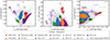 |
Fig. 1. Local sample of Gaia DR3 stars in different dynamical spaces (panels), classified into different groups (indicated by colour) by Dodd23. The panels show the spaces of energy and the vertical and perpendicular components of angular momentum used in Dodd23 to identify the Halo groups. The Disc group (purple) is kinematically selected with a Toomre velocity cut; the rest of the structures are found in the complementary kinematically selected Halo. In the plot, scatter points representing the Disc group have been down-sampled by a factor of 500, whilst the population in the legend is the total population of Disc stars. |
2.2. Crossmatched sample
As an additional test dataset, we create a sample of 6D stars using the 5D Gaia dataset, also within 2.5 kpc, crossmatched with a collection of other surveys providing vlos. This sample will allow us to test our methodology with stars entirely outside the RVS catalogue and a comparison with the results of Naik24. We include crossmatches of APOGEE DR17 (Majewski et al. 2017; Abdurro’uf et al. 2022), LAMOST DR7 low and medium resolution (Cui et al. 2012; Zhao et al. 2012), GALAH DR3 (Buder et al. 2021), and RAVE DR6 (Steinmetz et al. 2006; Kunder et al. 2017).
We process the data the same as our RVS sample, applying the same 2.5 kpc distance cut and similar quality cuts. We still require an error on the crossmatched error vlos less than 20 km s−1, but do not require (GRVS − G) < − 3 or a signal-to-noise spectra cut. We remove stars that are already in our 6D RVS dataset and those that are unbound.
These selections give 1 455 638 total stars; 4618 from RAVE, 35 824 from APOGEE, 22 390 from LAMOST MRS, 1 381 077 from LAMOST LRS, and 11 729 from GALAH; this sample is dominated by LAMOST LRS. Using a 210 km s−1 Toomre velocity cut, this sample is classified into 1 425 886 Disc stars and 29 737 Halo stars. Halo stellar groups are defined using the Dodd23 sample and a Mahalanobis distance of 2.2 (see Dodd23 for further details).
3. Density in action-angle space
This work uses axisymmetric action-angles to describe how stars are dynamically distributed. In action-angle space, (J,θ), the actions J = (JR,Jz,Jϕ) describe the orbit, and the angles θ describe where the star is along the orbit. The radial action JR and vertical action Jz quantify the radial and vertical oscillations of orbit, respectively, whilst the tangential action Jϕ is equivalent to the z component of angular momentum, Jϕ = Lz. The corresponding angles increase linearly with time modulo 2π as the orbit completes an oscillation in the respective dimension (see further details in Binney & Tremaine 2008).
In a phase-mixed galaxy, stars are spread out throughout their orbits, uniformly distributed throughout the (2π)3 volume of angle-space. The density in action-angle space is then directly proportional to the density in action space, divided by the volume of angle-space within which it is distributed:
 (2)
(2)
It is this assumption and effective reduction in dimensions that simplifies our methodology and improves the relationship between the observable 5D coordinates and the likely vlos. In the following Sect. 4, the density F(J, θ) is related to the likelihood of an individual star’s orbits.
3.1. Selection function correction
Our sample of 6D stars suffers from several selection effects that distort the observed distributions of dynamical properties from their true distributions. For a star to be in our sample, it must be: first, in the Gaia RVS catalogue; second, within 2.5 kpc of the Sun; and third, satisfy our quality cuts. Only orbits that enter our solar neighbourhood of 2.5 kpc can be observed; a circular orbit at 5 kpc or 11 kpc will never be seen. For this reason, our estimation of the orbital space in regions beyond our 6D sample’s 2.5 kpc distance limit is inherently incomplete, and our methodology cannot be correctly applied to stars outside our local region.
 (3)
(3)
Even if the Galaxy is perfectly phase-mixed, our sample of observed stars will not be uniformly distributed in angle-space. The solar neighbourhood selection in physical space corresponds to restricted regions of the angle-space that depend on the orbit’s nature. These regions are a fraction of the total (2π)3 volume and are equivalent to the fraction of time a star on an orbit is observable. Furthermore, due to the effective magnitude cut of the Gaia RVS selection function, our sample is biased towards observing more stars closer to us. At greater distances, we see only the intrinsically bright members of the stellar population, whereas at closer distances, we see a larger fraction of the stellar population.
Combining our selection effects, the action distribution that we observe, Fobs(J), is changed from the true action distribution F⊙(J) of the stars that cross the solar neighbourhood. We denote the expected observable fraction of a typical Halo stellar population on an orbit J as τ(J). The observed action distribution Fobs(J) is then:
 (4)
(4)
For example, if there are 1000 stars on an orbit that crosses the solar neighbourhood, and the expected observable fraction is τ(J) = 1/100, we expect to observe only 10 stars on average. The 1000 stars are approximately evenly spread in angle about the orbit, the majority in different parts of the Galaxy, and cannot be observed. From an observer’s perspective, we see the inverse; we observe 10 stars and statistically expect there to be 1000 stars upon that orbit. We must estimate τ(J), then F⊙(J) can be approximately recovered from Fobs(J) as:
 (5)
(5)
where the inverse fraction of time is written as the correction weight w(J), and the corrected observed action distribution  . We emphasise that this approximation only holds for orbits that cross the solar neighbourhood and are possible to observe (τ(J)≠0).
These weights can be considered a correction to unbias Fobs(J) from our observational, solar-centric view of our Galaxy. Combined with our phase-mixed assumption, the underlying phase-space density F(J,θ) can be estimated3 using  ), for orbits J that cross the solar neighbourhood. We briefly overview of how τ(J) is estimated below; for further technical details of the calculation, see Appendix A.
First, for an orbit J, we sample many physical points along its trajectory. Next, we define a typical halo stellar population with an isochrone, using a Chabrier (Chabrier 2003) Initial Mass Function and an alpha-enhanced BaSTI isochrone (Pietrinferni et al. 2021), with a metallicity of [Fe/H] = −1.1 and an age of 11 Gyr. Then, the probability of observing a star of a given magnitude and colour from the stellar population at the sampled positions is evaluated. This probability is estimated using the dust maps of Lallement et al. (2022), photometric corrections of Gaia Collaboration (2018b), and the RVS selection function of Castro-Ginard et al. (2023). Observational uncertainties and the corresponding quality cuts are estimated using the PYGAIA4 software package. Finally, by averaging over the defined halo stellar population and over the points around the orbit, the expected observable fraction τ(J) of stars upon the orbit J is found.
3.2. Density estimation
Using the phase-mixed assumption and the selection function correction, finding the underlying phase-space density F(J,θ) reduces to evaluating the corrected density  . We model this as a collection of points and weights [Ji,wi], from which we want to estimate the density at arbitrary J5. This is numerically challenging, as the density varies by orders of magnitude throughout the action space.
We choose to use a Modified Breiman Estimator (MBE), as described in Ferdosi et al. (2011) and used in other works to estimate action space density (Sanderson et al. 2015). The MBE uses an Epanechnikov kernel with an adaptive smoothing length for each point to ensure a smooth density. This method is further modified to include the selection function correction weights and a scaled action space to ensure a smooth density for all groups. Furthermore, to help with the numerical calculation, we first transform from action space (JR, Jz, Jϕ) to the space of  . The method is described in detail in the appendix (see Appendix B).
This methodology of weighted corrections and smoothing does have limitations. We cannot estimate the density in regions of action space where we do not have any stars. Lower binding energy orbits (equivalently larger action) have longer orbital periods and spend less fraction of their time in the solar vicinity, and so get larger correction weights. This region is also where there are fewer stars due to the nature of the action distribution of the halo. As a result, in these regions, the observed distribution is very poorly sampled and hence more stochastic, relying on the few observed stars to receive a high correction weight, which is then given a very large smoothing. These areas do not give very reliable density estimates for the halo.
4. Method
A star is observed with 5D coordinates denoted u: parallax, position on sky, and proper motions. Given this information, we want to infer the probability of the star having a particular vlos, the probability density function (PDF) denoted p(vlos|u). The PDF can be expressed as:
 (6)
(6)
As only the vlos is varied, the normalisation factor of p(u) can be dropped, provided that, at the end of the calculation, the PDF is renormalised so that it integrates to unity over the space of possible vlos.
The transformation from observed space (vlos,u) to 6D Galactocentric cartesian space (x,v) uses fixed solar parameters. The Jacobian factor is independent of the vlos, as the vlos can be considered as a velocity component of a rotated, shifted, and boosted cartesian frame. Again, this Jacobian factor can be treated as a normalisation factor and dropped:
 (7)
(7)
The transformation between (x, v) and (J, θ) is canonical, and so:
 (8)
(8)
Here, F(J,θ) is the distribution of all stars in action-angle space. Collecting everything together, it follows that:
 (9)
(9)
The normalised vlos PDF is then:
 (10)
(10)
where the total normalisation factor is:
 (11)
(11)
depending on the path through the action-angle space set by the 5D coordinates. This path is evaluated at vlos between the positive and negative values that correspond to the vlos that brings the star’s total speed to escape velocity.
Using results from Sect. 3, by assuming that Galaxy is phase-mixed, the density in (J, θ) space can be assumed to be directly proportional to the density in action space F(J) (Eq. (2)). For J that cross into our solar neighbourhood, this can be approximated by our observed sample of stars, corrected for selection effects,  (see Sect. 3.1, Eq. (5)). Then:
 (12)
(12)
Note that this only holds for orbits J that cross the solar neighbourhood due to the selection of our observed 6D sample. If the 5D stars position lies within our 2.5 kpc selection solar selection, this is assuredly the case. The following descriptions refer to the path and density as within action space, but this is a generalisation of assuming a phase-mixed action-angle space.
The shape of a star’s vlos path through the action space depends on the observed coordinates u. The lowest point in action space (nearest to the origin) approximately corresponds to the minimum possible energy of the orbit. As the potential energy depends on the fixed position, the minimum total energy is where the vlos minimises the kinetic energy. This value is not necessarily at vlos = 0 due to the Sun’s motion in the coordinate transformation from heliocentric coordinates. As the magnitude of vlos increases to become the dominant component, the total velocity and kinetic energy also rise, the actions increasing until the orbit becomes unbound, with E > 0. Here, the actions are undefined, and the density and corresponding likelihood are zero.
An example of applying our method to a star from our 6D sample can be seen in Fig. 2, depicting the vlos path through action space, and the corresponding (total) PDF in Fig. 3. The path that this particular star takes crosses the region of action space associated with GES, but also traverses the region of Sequoia and Ungrouped Halo. In this case, the region of GES is the densest, and so the star is most likely to have a vlos corresponding to an orbit consistent with GES. For this chosen example, this is close to the true vlos of the star.
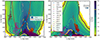 |
Fig. 2. Our sample of 6D Gaia DR3 RVS stars in action space, classified into different groups of Dodd23 (indicated by colour). The Ungrouped Halo stars are represented by smoothed density, as indicated by the colours and contours in the colour bar. This density, and those of the individual groups, are corrected for selection effects (see text). Across the space is an example path (red line) of a 5D star through action space found by varying an assumed vlos, with values indicated in the legend. The corresponding PDF can be seen in the following Fig. 3. This example star is a GES member from the 6D Gaia RVS sample, with the true vlos and the corresponding point in action space marked by a square. |
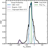 |
Fig. 3. PDFs of vlos, calculated from a 5D star’s path in action space (see Fig. 2). The thick black line total PDF shows the total density. This total can be decomposed into contributions from different groups, denoted by different colours. The probability that the star belongs to these different groups can be found by integrating the area under the respective lines, shown in the legend. As a star from the 6D sample, the true vlos is marked in green, and it is known that it is a GES member. Our method finds a 63% probability of belonging to GES but could also belong to Ungrouped Halo or Sequoia. |
4.1. Group membership
The total density can be decomposed into contributions from each of the stellar Halo substructures’ distributions:
 (13)
(13)
The individual group’s PDFs are then normalised using the integral of the total PDF:
 (14)
(14)
so that the total PDF integrates to one. The integral under the group’s individual PDFs gives the membership probability of the star with 5D coordinates u belonging to each group g:
 (15)
(15)
By construction, these probabilities sum to one; the stars must belong to one of the groups (including the Ungrouped Halo). The total Halo’s PDF and probabilities are simply the sum of all groups except the Disc.
In action space, there is a small region of overlapping Halo and Disc where a given orbit’s velocities within the solar neighbourhood can variously fall just above or below the 210 km s−1 Toomre velocity cut. To ensure consistency with our initial kinematic definitions of Halo and Disc, a Toomre velocity cut is applied to the tested stars. For a given vlos, if the star has a VToomre > 210 km s−1, then any density from the Disc is moved to the HTD, or Ungrouped Halo if there is not already contribution from the HTD, with the Disc density set to zero. Similarly, a star with VToomre < 210 km s−1 has any contribution from the Halo components moved to the Disc. This criteria only affects a minimal selection of orbits but prevents the inference of a Disc or Halo membership that does not satisfy our kinematic definition.
The individual group PDFs and probabilities can be seen for the example 5D star in Fig. 3. As stated before, GES is the dominant contribution to the density across the path for this star, with a probability of 63%. However, there are also probabilities that the star belongs to Sequoia or the Ungrouped Halo. There is zero probability of this star belonging to the Disc as there is no possible disc-like orbit for any vlos because the path in action space is far from the region associated with the disc.
4.2. Phase-clumped and partially phase-mixed substructures
Our methodology can be improved by recognising that not all groups are phase-mixed within the observable volume. If a structure is truly phase-mixed, then the number of positive and negative values of its stars’ radial and vertical velocities (vR, vZ) are expected to be approximately evenly distributed (where R is the radius in the plane). There should be approximately the same number of stars traveling up through the z = 0 plane as traveling down, and as many stars going towards and away from the Galactic centre.
In (vR, vZ) space, this would be roughly an equal number of stars in each positive-negative quadrant for each group. Not all of the Halo substructures are phase-mixed; the clear exceptions can be seen in velocity space in Fig. 4. The following groups are referred to as phase-clumped: ED-2 (with a particularly tight velocity spread), ED-3, ED-4, ED-5, ED-6, LRL64, and Typhon. These groups also show tight grouping in the tangential component of velocity (by construction).
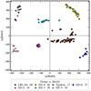 |
Fig. 4. Stars of un-phase-mixed groups in radial and vertical velocity space (in Galactic cylindrical coordinates). If the groups were phase-mixed, there would be a roughly equal number of stars from each group in every quadrant. Whilst not every group is in a single quadrant, none are consistent with being evenly distributed. |
The stars in these groups are phase-clumped together in a smaller volume within the larger observable volume. As a result, these structures have higher density in some parts of the angle-space but smaller, or zero, in the rest. For these groups, Fg(J, θ) is not well estimated by assuming that the stars distributed as Fg(J) are spread uniformly in angle-space. Instead, we may assume these groups are uniformly distributed in a restricted volume of angle-space.
The restricted volume is defined by making an additional velocity selection, requiring that the velocity of the evaluated point be within a characteristic velocity length scale of known group members in velocity, (vR, vZ, vϕ).
 (16)
(16)
The velocity length scale σv is estimated for each group by considering the largest range  of the distribution of different absolute velocity components, and can be seen in the legend of Fig. 4. These length scales are deliberately chosen to be generous so as not to be overly restrictive while effectively describing the space. These velocity criteria are applied as an additional selection function when calculating the correction weight for stars in the phase-clumped groups, effectively reducing the volume of angle-space that the star can be observed in and increasing the correction weight.
When evaluating Fg(J,θ), the position in velocity space is additionally checked:
 (17)
(17)
If the velocity satisfies the velocity cut, the group’s contribution to the density is included; otherwise, it is zero. In later analysis, this additional phase-clumped step is found to improve the recovery of these structures and reduce contamination from non-group members. This process is only applied to the identified phase-clumped groups.
5. Testing vlos predictions
We now test our methodology on both our 6D samples. Every star’s 5D information is used to predict a vlos PDF and group membership probabilities. These predictions can then be evaluated using the true vlos and the group membership of Dodd23. For the RVS sample, the stars define the action-angle density used within the method. Therefore, when testing a star from this sample, the density contribution from its own true point is removed when evaluating the density along its path in action space. This measure ensures that the test is not biased favourably, with an advantage that cannot be replicated when applying to true 5D stars. In practice, this makes a negligible difference due to the density smoothing.
In the following tests and discussions, the samples are frequently decomposed into Halo and Disc stars for separate analysis. We find that predicting the vlos for these kinematic groups is very different, as it is generally far easier to constrain a Disc star to a Disc orbit than a Halo star to a specific Halo orbit (as shown in the following section). Without considering these groups separately, the total sample and results are dominated by Disc stars, masking any meaningful study of the Halo.
The statistical accuracy of the inferred vlos PDFs can be quantified by considering the cumulative distribution function (CDF, defined H) evaluated at the true vlos:
 (18)
(18)
If the predicted PDFs are genuinely accurate and unbiased, the total distribution of HTrue should be uniformly distributed6. Similarly, a subselection in any quantity independent of vlos, such as distance and positions, should be uniformly distributed.
However, selecting kinematically defined groups of stars includes an implicit selection on vlos and is, therefore, a biased selection of HTrue. Instead, cumulative distribution values are calculated from a group’s own PDF rather than the total PDF. These CDF values are then selected and calculated with the knowledge that they are true group members and are statistically expected to be distributed uniformly. The total distribution can then be decomposed into separate Disc and Halo distributions, ensuring that the predicted PDFs are statistically accurate for both groups of stars.
The distributions of the cumulative values for the total Gaia RVS sample7 are plotted in Fig. 5, alongside the Disc and Halo subsamples. These distributions are nearly, but not quite, uniform. The total is, as expected, dominated by the Disc distribution, which shows a clear slight asymmetric trend. We attribute this trend to disequilibrium within the Disc due to the correlation between dynamical structure and small systematic under and overestimating of vlos throughout the solar neighbourhood (see Appendix C for details). This disequilibrium violates our assumptions of phase-mixed, axisymmetric equilibrium. The Disc PDFs are very narrow, and as a result, these minor biases in the CDF only correspond to a few km s−1 in vlos and are not detectable in other tests and analyses.
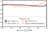 |
Fig. 5. Distributions of CDF values H(vTrue), calculated from the true vlos of the stars and the PDFs of our method, for each star in our Gaia RVS sample. If all assumptions and the PDFs are correct, these values should be distributed uniformly. We plot the total distribution of all stars and the distributions of the Disc and Halo stars (with CDF values corresponding to their respective PDFs). The total statistical error Δ% of our PDFs can be estimated by integrating the difference between the found and true uniform distribution. |
The Halo distribution shows a slight excess of stars near cumulative values 0 and 1, indicating that more true vlos values are in the tails of the predicted PDFs than is statistically expected. The tails of the PDFs are typically regions of high vlos, corresponding to areas of high energy and action. This excess suggests that the density in these regions is slightly underestimated, likely due to the difficulty in reliably estimating the density in these areas (see Sect. 3.2).
The differences between our results and the correct uniform distributions are quantified with two statistics. First, following Naik24, the total absolute area between the found distribution f(H) and the ideal uniform distribution:
 (19)
(19)
where Δx is the width of the bins. Note that this statistic depends upon the choice of binning and Poisson noise in smaller samples, such as the Halo sample. In addition, the KS statistic ΔKS describes the maximum difference between the cumulative distributions, scaled by a factor of 100 for convenience:
 (20)
(20)
This quantity has the advantage that it can be calculated without a choice of bins and is more robust to small number statistics.
For the Disc distribution, we find Δ% = 0.85% and ΔKS = 1.4, whilst the Halo has values of Δ% = 0.95% and ΔKS = 2.0. These statistics confirm that both populations are well recovered, without strong systematic biases.
5.1. Constraining vlos
Whilst the predicted PDFs can be considered statistically consistent with the truth, that does not necessarily mean that they effectively constrain the likely vlos of a given star. The predictive power of our vlos PDFs can be quantified by defining the uncertainty in our vlos estimate:
 (21)
(21)
where vX% corresponds to the vlos that is X% of the way through the cumulative distribution of a given PDF, X%=H(vX%|u). The smaller the σPDF range, the more constraining the PDF, and the smaller the uncertainty on a predicted vlos.
The distribution of σPDF for the RVS sample is plotted in Fig. 6, split into both the true Disc and Halo. Stars belonging to the Disc are well-constrained, with a median σPDF of 26 km s−1, slightly smaller than the velocity dispersion within the thin disc (Bland-Hawthorn & Gerhard 2016). This average uncertainty is the same value as the total sample (which is dominated by the disc) and similar to the results of Naik24. As shown in the following Sect. 6, the overwhelming majority of Disc stars are correctly identified. Stars belonging to the general Halo are far less constrained, with a larger median σPDF of 72 km s−1.
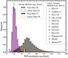 |
Fig. 6. Distributions of σPDF (defined as half the 84%−16% vlos values) of the PDFs predicted by our method. The sample is split into Halo and Disc stars, whose normalised histograms of the true decomposition are plotted with solid-filled colours. The likely decomposition, defined by the probability of membership greater than 80%, is plotted with lines. The median values for the distributions for stars belonging to different groups (based on Dodd23) are shown in different colours. |
However, stars likely to belong to substructure within the Halo are typically better constrained, as can be seen in the median σPDF values of likely members (defined as membership probability greater than 80%). In general, the likely members of smaller substructures have much smaller σPDF values, as they are so narrow and dense in the phase-space that only a small range of vlos corresponds to a matching orbit. The groups that are broad in action space typically have members with wider, less constraining PDFs. The group with the largest median σPDF is Sequoia, which is reasonably broad in action space and has a small membership for its size. These combined factors result in a lower density in action space, leading to less dominant, less sharply peaked, and less constraining PDFs.
The sample is additionally decomposed into likely Halo and Disc members (defined at a membership probability above 80%). There is a noticeable deviation at lower uncertainty between the distributions of true Halo stars and those that are found likely to belong to the Halo. A small fraction of Halo stars are being misattributed to the Disc with high probability, being predicted by narrowly constrained PDFs corresponding to disc-like orbits.
5.2. Predicting vlos
Predicting a single value estimate for the vlos of an individual star can be difficult, as many of the star’s PDFs are complex and multipeaked and, therefore, are not well summarised by a single value. It is more robust to marginalise over the entire vlos distribution, as discussed in the following Sect. 5.3. If it is necessary to distil the PDF into a single vlos estimate, there are two obvious choices: the vlos corresponding to the PDF’s peak value (Vmax) or the vlos corresponding to the median value of the PDF (Vmed). We then define the difference between our predictions and the true vlos value as Δv = |vPredict−vTrue|.
The distributions of the differences Δv for our predictions Vmax and Vmed are plotted in Fig. 7, decomposed into Disc, total Halo, and grouped Halo (stars belonging to substructures). The top panel shows the results for the RVS sample, and the bottom shows similar results for the crossmatched sample, for which we additionally have the results of Naik24. These results follow the distributions of Fig. 6, where the Disc have, on average, the smallest differences Δv. The general Halo stars have comparatively larger differences Δv, but likely substructure members can be found with greater accuracy. We find that Vmax and Vmed give similar results on average, although the individual estimates for stars can vary. The Vmax estimates perform marginally better for well-constrained PDFs with a single dominant peak, typically found in PDFs of likely substructure members. However, Vmax estimates differ more from the true vlos than Vmed estimates on average for less well-defined PDFs.
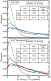 |
Fig. 7. Distributions of the difference between vlos predictions and the true vlos across different subsamples of the Disc, the total Halo, and the stars belonging to substructure in the Halo. The top panel sample is from the Gaia RVS catalogue and includes vlos estimates our PDF’s the median and peak maximum values. The bottom panel shows a sample of stars from surveys crossmatched with Gaia and includes vlos estimates from Naik24. The tables contain the median velocity error for the different velocity predictions across the different subsamples. |
To ensure that the differences between vlos estimates and the true value are statistically consistent with the expected uncertainty σPDF, consider Fig. 8. By binning stars in σPDF, the running median, 1σ, and 2σ of the differences between the predicted and true vlos within the bin are calculated, defined by the percentile ranges 16 − 84% and 5 − 95%, respectively. If the predicted uncertainties and vlos estimates are statistically accurate, the 1σ of the distribution within bins should equal the σPDF value of the bin itself. We find good agreement across the entire range of σPDF; the uncertainties in our vlos PDFs are statistically consistent with the true differences between our prediction and the true value.
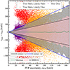 |
Fig. 8. Uncertainty in our predicted vlos PDFs against the difference between the true value vTrue and our predicted line-of-sight velocity vmax. True Disc stars are plotted in purple, downsampled by a factor of 1000, the true Halo stars that are determined to be likely Halo stars by our method (probability greater than 80%) in orange, and true Halo stars that are misdetermined to be likely disc stars in red, both downsampled by a factor of 2. The median line and shaded regions indicate the binned running median and 1σ and 2σ values of the total distribution, defined from the 16%−84% range. If the predictions are unbiased and the predicted PDF uncertainties accurate, the binned 1σ and 2σ values regions are expected to follow the value of their own corresponding bin, plotted in solid black and blue lines. |
By considering the subsamples of stars, indicated by colour in Fig. 8, the same patterns as before can be seen. The Disc stars are well recovered and constrained, whilst the majority of the Halo stars are identified with greater σPDF that is statistically consistent with the true differences between the predicted and the true vlos values. However, a small population of true Halo stars is misattributed to the Disc (in red). These stars are predicted with small vlos uncertainties, but, in reality, the differences between our predicted and true vlos values are large.
5.3. Marginalising over vlos
For a given star, the PDF of any other dynamical quantity normally calculated using 6D position-velocity can be found using the inferred vlos PDF. Whilst this can be found analytically, in practice, we find it is easier to sample the stars’ vlos PDFs numerically. For each star, we sample vlos points on a linear space, which we use to compute the 6D position-velocity and calculate dynamical quantities such as IoM. At each of these vlos points, the star’s vlos PDF defines a weight, normalised so that across the vlos points for a given star, the weights sum to one. Across all stars, vlos distributions can then be marginalised over by using these weighted contributions to distributions. By instead using the PDFs of individual subgroups, whilst still normalising by total, the dynamical distributions of the subgroup can be found.
This method is applied to recover the 1D dynamical distributions of the total Halo and Disc in Fig. 9. The action distributions and vlos are all in excellent agreement with the original distributions. The velocity components are recovered reasonably well, but the halo distribution shows some slight deviations from the true distribution. Most notably, in the distribution of vR, the true Halo shows distinct asymmetry, with slightly more stars falling towards the Galaxy’s centre. This asymmetry could possibly be the influence of the bar (Monari et al. 2019) or suggest incomplete phase-mixing. The Halo stars are not exactly uniformly distributed in angle-space, as our methodology assumes, and so this minor feature is not recovered. There is a small excess of stars predicted at near Lz ≈ 0, but we find it is not significant enough to affect other results.
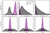 |
Fig. 9. Distributions of various dynamical quantities of the Disc and Halo samples, defined kinematically by VToomre > 210 km s−1. The solid distributions are the original 6D distributions, and the lines are the recreated distributions from the 5D of the 6D sample by marginalising over the likely vlos PDFs inferred by our method. The top panel depicts the components of action space, and the bottom panel the components of velocity. |
This technique can also recover higher dimensional distributions and dynamical properties of individual Halo substructures, as shown in Fig. 10. The general velocity structures of our groups are recovered very well, with additional smoothing. The smaller asymmetries and overdensities within the velocity distributions are not recovered, indicating a more complex phase structure in angle-space than our assumed uniform distributions. For the phase-clumped groups in the bottom panel (excluding the phase-mixed HS), our additional step of explicitly selecting phase-clumped groups in velocity space ensures that clear velocity structures are well recovered. The velocities recovered without this additional step can be seen in Appendix D.
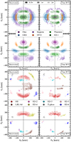 |
Fig. 10. Cylindrical velocity distributions of the different groups, as recovered by our methodology (lefthand side) against the true distributions (righthand side). Different stellar groups are represented by different colours, with the opacity of the colour representing the (0.5σ, 1σ, 2σ) levels (equivalently the 38%, 64%, and 95% regions). The groups are split into two separate subpanels, with the majority of phase-mixed groups in the top set and phase-clumped groups, with the addition of the Helmi Streams to allow the groups to be visually distinguished, in the bottom set. |
6. Predicting membership probability
An advantage of our methodology is that it provides the membership probabilities of a star belonging to the Disc, Halo, or a specific substructure within the Halo. These probabilities can then be used to select a sample of stars belonging to a desired substructure. We now explore the statistical accuracy of our membership probabilities and how effectively they can be used to select high-quality samples of likely members.
The distribution of the probabilities for each group can be seen in Fig. 11. The exact membership probabilities for an individual star have a complex dependency on the exact path taken through action space. However, there are a few general trends. Consider the probability distributions of Disc and total Halo stars, whose probabilities, by definition, sum to one. Most stars’ membership probabilities between these two groups are very polarised. The Disc has overwhelming population numbers and density, and as a result, if a star can possibly have a Disc orbit for a given range of vlos, it is very likely to be a Disc star. If the star cannot be on a Disc orbit for any vlos, it must be a Halo star. There are proportionally very few Disc stars with a low probability of Disc membership, but a population of Halo stars is mistaken for Disc.
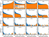 |
Fig. 11. Distributions of membership probabilities of our individual groups (separate panels), calculated with our methodology. The distribution of the membership probabilities of every star is plotted in blue, and the true group members in orange. The first two panels depict the Disc and the total Halo. The total Halo is decomposed into individual structures and Ungrouped Halo. By construction, a star’s probabilities of belonging to the Disc or the total Halo sum to one, and the total Halo membership is then decomposed into belonging to structures or Ungrouped Halo. |
Within the Halo, the different substructures have very different member probability distributions. These distributions depend on the structure’s density and location in action space. A defining feature is the lowest energy point of the action path or Emin. The lower a 5D stars’ Emin, the deeper the vlos path goes into action space, and the greater the range of possible vlos and orbits. In general, this correlates with larger uncertainties σPDF and membership probabilities are split between different groups.
Consider Thamnos and ED-1 groups at a low-energy position in the space. Both groups have few stars with membership probabilities greater than 50%, as any star that could be a Thamnos or ED-1 member could also have an orbit at higher energy and belong to another substructure or the Ungrouped Halo. The stars’ path in action space will traverse these structures, which translates directly into alternative membership probabilities.
The smallest phase-clumped structures, such as ED-2, are very dense in phase space. Few stars cross their region of phase space, but those that do are likely to be higher probability members unless the action path also traverses an even denser structure, such as the Disc. On the other hand, The Ungrouped Halo has no high-density region in action space but is instead spread over a large portion of the space, including higher energy areas. All stars’ vlos path in action space will cross a section of this high-action space before the orbit becomes unbound. As a result, all stars have a nonzero probability of belonging to the Ungrouped Halo.
6.1. Expected populations
The statistically expected population number of a group in the sample can be calculated by considering the membership probabilities across the entire sample of stars:
 (22)
(22)
where  is the probability that star i belongs to group g. The uncertainties in this estimate can be calculated by randomly drawing a group population based on the probabilities many times (we use 10 000), then taking the median and 16 − 84% percentile ranges. The accuracy of this method can be studied by comparing the estimated population to the true population (see Fig. 12).
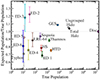 |
Fig. 12. Expected populations of the stellar groups of our 6D RVS sample, calculated using membership probabilities assigned by our method, compared to the true population (based on Dodd23 groups). The error bars are estimated by redrawing the populations based on the membership probabilities of the stars. |
The ratio between the Halo and the Disc is approximately correct, with 99.6% of stars expected to belong to the Disc, with the total Halo overestimated by only ∼4%. The population sizes of the substructures are typically recovered within the expected statistical uncertainties. Overall, our groups’ expected populations are within 30% of the true population, with a slight bias to underestimate smaller groups. The smaller groups have more significant fractional uncertainties due to poor sampling and a larger Poisson effect. Even groups without many high-probability members, such as Thamnos and ED-1, have approximately the correct expected population due to having many low-probability members.
6.2. Purity, completeness and selecting a sample
A sample of stars likely belonging to a group can be selected with a cut in minimum membership probability, pmin (see Fig. 11). The quality of the selected sample for a given pmin can be quantified by defining the purity and completeness as:
 (23)
(23)
 (24)
(24)
where Ng is the true population of the group in the total sample, Ng(pmin) is the population above the pmin probability cut, and  is the true population above the pmin probability cut.
The effects of choosing different probability cuts are explored in Fig. 13. Increasing the pmin of a sample increases the purity but reduces the completeness and overall sample size. This behaviour at a given pmin depends on the distribution of membership probabilities for the selected group (Fig. 11). Groups with many correct high-probability members can be recovered well, with high purity and completeness.
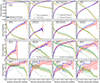 |
Fig. 13. Plots depicting effects of increasing the minimum membership probability upon the purity and completeness of the selected sample of a group. For each group (panel), increasing the probability cut on membership probability (x-axis) increases the purity of the selected group, but decreases the completeness (y-axis). We plot the true purity and completeness, and the expected purity and completeness calculated from the probability distribution. For groups that show evidence of being phase-clumped, we also plot the purity and completeness calculated without the additional phase considerations (see Sect. 4.2). |
For an actual 5D sample without observed vlos, the true purity and completeness of a selection will be unknown, and they cannot be used to guide an appropriate selection of pmin. Instead, the expected purity and expected completeness of a given sample can be calculated using the expected populations at a given pmin cut instead of the true populations:
![Mathematical equation: $$ \begin{aligned} \langle N_{\rm g}\rangle (p_{\rm min}) = \sum _{i\in \left[p_{\rm g}^{i} > p_{\mathrm{cut} }\right]}p_{\rm g}^{i}. \end{aligned} $$](/articles/aa/full_html/2024/10/aa50745-24/aa50745-24-eq33.gif) (25)
(25)
The uncertainties in these values can be found by stochastically drawing samples based on the membership probabilities, similar to those found for the total expected populations. These expected values are plotted as shaded regions in Fig. 13. Generally, the expected purity matches the true purity within the expected scatter, suggesting that the purity and completeness of a given sample can be predicted.
When selecting a sample of 5D stars, the ideal choice of pmin depends on the intended analysis, which will typically require a certain purity or number of stars. The trade-off between expected purity and completeness can be seen directly by considering the purity of a sample at a given completeness, parameterised by the probability cut pmin as a recovery curve, plotted in Fig. 14. These curves concisely describe how well a given group can be recovered, with the best-recovered groups giving higher completeness for a given purity. For the smaller groups (rightmost panel), a purity of 80% can be taken while remaining above 50% complete. For some poorly recovered groups, such as ED-1, Thamnos, and the HTD, any sizeable sample taken will inherently be impure.
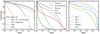 |
Fig. 14. Curves describing the effective recovery for our different groupings, using the expected purity and completeness of a given probability cutoff. These curves describe the inherent trade-off of choosing a sample of stars; the higher the purity, the lower the completeness. Better recovered structures have a higher completeness for a given purity. In the first panel, we additionally plot the recovery curve from making a transverse sky velocity cut (see text for details). |
7. On comparisons and selections
7.1. Comparison to Naik24
Arguably, the closest current work to our predictions of vlos for individual 5D stars is Naik24. This work used machine learning on inputs of the 5D observable coordinates, applied to a large sample of stars spanning much greater distances than our own 2.5 kpc limit. In theory, the method of Naik24 does not make assumptions of phase-mixing, axisymmetry, or the Galactic potential and can predict disequilibrium structure. They successfully recover vlos with a typical uncertainty of 25 − 30 km s−1 and demonstrate that their PDFs are statistically consistent with a value of Δ% = 1.4%. Since they do not explicitly distinguish between Halo and Disc members, their results can be expected to be dominated by Disc stars. Their uncertainties are very similar to our own predictions for Disc stars, which, on average, are slightly smaller than the velocity dispersion of the thin Disc.
To compare vlos predictions, we use our 6D Crossmatched sample, containing approximately 30 thousand Halo stars. Using the provided median vlos estimate of Naik24, denoted VNaik, we show the distribution of the differences  for the different subgroups with the red curve in the bottom panel of Fig. 7. We see similar distributions of the differences Δv in the Disc and Halo samples. However, the stars belonging to Halo substructures do not show smaller differences Δv compared to the total Halo, as we find with our velocity estimates. This could suggest that not all individual substructures have been effectively modelled.
To test this more explicitly, the vlos prediction differences Δv of our Vmed results and those of Naik24 are directly compared for members of different structures in Fig. 15. Generally, for larger structures, such as the Disc, GES, Thamnos, and the HTD, we see very comparable results. However, for smaller structures, our prediction differences Δv are significantly smaller than those of Naik24, with the most significant change for ED-2. As a structure, ED-2 has few members spread out very thinly over the observable space, and so it is difficult for methods like Naik24 to recover, unlike our IoM-based methodology.
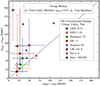 |
Fig. 15. Comparisons between the differences between the true vlos and the predictions of our methodology and Naik24, with samples decomposed into different halo substructures. We include all stars from the true groups, plotted with triangles, and true likely members with membership probability greater than 50%. Only groups with more than 4 likely members are plotted. The points and error bars represent the median and the 16% and 84% percentiles of the distribution, respectively, for the likely groups. These results use the crossmatched 6D sample described in the main text. |
When the stars are further restricted to those that we find likely to belong to a structure (pmin > 50%), we see improvement in both estimates. This improvement is expected for our own results, as almost by definition, the true stars that we find likely members have been well recovered. The fact that the results of Naik24 also improve suggests that some common areas of the 5D parameter space are better recovered.
7.2. Comparison to Mikkola23
The work of Mikkola23 models the local (within 3 kpc) velocity distribution of a 5D Gaia sample. They split their sample using a VTan > 200 km s−1 cut to divide the Disc and Halo, with a colour-magnitude diagram selection to focus on the Halo blue sequence (Gaia Collaboration 2018b). In the Disc, their methodology successfully finds velocity substructure, including new likely structures within the 5D dataset. In our work, we make no distinction between moving groups of the Disc, instead focusing solely on the Halo.
In the Halo, their predicted velocity distributions show the signature of several prominent accreted structures, which also appear in their recovered action space distributions. By finding the total density within these velocity features, they estimate the population of substructures of the 5D sample. In theory, the methodology can also be extended to attribute individual stars to particular structures (e.g., Cronstedt 2023) but we cannot currently directly compare predictions for single stars.
7.3. Selecting a halo sample with vtan
It is common practice to define a Halo sample 5D stars using only the transverse velocity of a star across the sky, defined:
 (26)
(26)
where d is the heliocentric distance, and μ is the amplitude of proper motion,  . The relationship between VToomre and VTan can be seen in the top panel of Fig. 16.
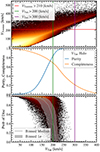 |
Fig. 16. Plots of the dependence of Halo and Disc properties on VTan, the on sky velocity. The top panel shows the distribution of VTan against VToomre, where the horizontal red line depicts the VToomre cut used to kinematically define our Halo and Disc Samples. The middle panel shows the purity and completeness of the sample; for the common VTan > 200 km s−1 halo selection, the sample is 83% pure and 69% complete. The bottom panel shows the probability of the star belonging to the Disc, as inferred by our method. |
Any star with a large VTan is likely to have a large VToomre and can be assumed to be kinematically a Halo star. However, the selection on VTan neglects Halo stars that distinguish themselves from the Disc through high vlos. The halo selection cut typically used is VTan > 200 km s−1 (Gaia Collaboration 2018b; Mikkola et al. 2023), which selects a VToomre defined Halo with 83% purity and 68% completeness. A stricter cut improves purity but quickly reduces the completeness, as shown in the middle panel of Fig. 16. VTan > 300 km s−1 gives a sample of greater than 99% purity but only 21% completeness.
This technique makes an interesting comparison with our methodology, as Halo stars with low VTan should have orbits consistent with the Disc for small vlos. As expected, there is a clear correlation between higher VTan and decreasing probability of belonging to the Disc, as shown in the bottom panel of Fig. 16. We find that our methodology offers a marginally better way of defining a halo sample, with a slightly higher completeness for any given purity. A similar 83% purity selection has a completeness of 76%, an additional 8% sample size compared to the equivalent VTan > 200 km s−1 selection. The recovery curve from taking a varying VTan cut can be seen in the first panel of Fig. 14, and is below the recovery curve of our own results.
8. Discussion
This work has made several implicit assumptions about the nature of our Galaxy. Firstly, we have assumed that the Galaxy is well-modelled by an axisymmetric, static Galactic potential. Secondly, we have assumed that the stars are completely phase-mixed (or, for the phase-clumped stars, uniformly distributed within a reduced region of angle-space). These assumptions have allowed us to model the local stars effectively in action-angle space. We have found no strong biases or differences when testing our methodology with a different galactic potential to compute the actions.
To evaluate our results, we have been comparing our inferred membership probabilities to the initial labelling of Dodd23, originally made in the space of energy and components of angular momentum. Whilst these groupings are approximately consistent with regions of action space, there is typically a difference in the membership of individual stars under 10%. The groups with the largest membership difference are Thamnos, at 30%, and ED-1, at 20%.
Like any other kinematic selection, the groups of Dodd23 are inherently incomplete and contaminated. Notably, the Thamnos group is likely to contain large amounts of contamination. The area of phase space that Thamnos occupies at lower energy has several other overlapping groups, such as GES and splashed insitu stars (Belokurov et al. 2020). The “true” metal-poor Thamnos is probably far smaller but would require a more comprehensive chemical selection to improve the purity of the selection.
In general, selections of Dodd23, based on a Mahalanobis distance of 2.2, are likely to be conservative. This is particularly true for GES, whose population of selected members is proportionaly a smaller fraction of the total Halo than estimates of its stellar mass compared to the total Halo (Helmi et al. 2018; Lane et al. 2023). Furthermore, as a massive accretion event, the true members of GES are scattered wider in IoM space, and it is hard to make a pure or complete kinematic selection (Amorisco 2015; Koppelman et al. 2020; Carrillo et al. 2023).
8.1. Phase-clumped or phase-mixed
In our methodology, we have modelled groups identified as phase-clumped with an additional step to account for their non-uniform distribution in angle-space. To quantify the effect of this step, we compare our results to the methodology without this additional phase-clumped assumption. We find that the purity and completeness of the groups modelled as phase-clumped are higher than when modelled as phase-mixed (see Fig. 13). The phase-clumped modelling increases the membership probability of true members and reduces the number of contaminants.
This relative improvement is most evident when considering the most phase-clumped structure, ED-2. The true 6D Gaia RVS members form a neat stream travelling through the solar vicinity (see Fig. 17). The likely samples (using pmin = 50%) found assuming the structure is phase-clumped correctly recovers 27 out of 34 true members, with 5 contaminants, whilst the phase-mixed sample recovers only 15 likely members, with 4 contaminants. The phase-mixed sample contains a few obvious outliers, stars with likely velocities (defined using Vmax) that are misaligned with the stream. The contaminants of the phase-clumped sample seem to mostly lie outside the thin region of (R, Z) space that ED-2 inhabits, suggesting that an additional selection in physical space could improve the purity of the membership.
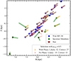 |
Fig. 17. Stars from our ED-2 samples in R − z space, with velocities indicated as trails. In blue are the true known members from our 6D Gaia RVS sample. In orange, the likely members of ED-2 inferred from 5D information, without known vlos, by our method. The velocities are predicted from the most likely vlos corresponding to the peak of the PDF. In red, the stars were inferred without using the additional phase information of ED-2 (described in Sect. 4.2). Both of these samples have been selected with a minimum probability of pmin = 50%, corresponding to an expected purity of 86% with phase information and 56% when assuming the structure is phase-mixed. |
However, it could be argued that this additional step risks overfitting these phase-clumped groups. It is possible that these structures are poorly sampled, and with a larger sample of stars, additional members could be found in different areas of velocity space. These new stars would be missed by our phase-clumped modelling’s strict velocity selection but would, in principle, be detectable with phase-mixed modelling (see Appendix D). Furthermore, stars on resonant orbits will not be well modelled by this methodology due to their distribution in angle-space. In our following paper, we will apply our method to a 5D Gaia sample, assuming the groups are phase-clumped to find high probability members. We will also apply our method assuming the groups are phase-mixed and search for new features in the velocity space.
8.2. Improving the method
Our methodology could be developed further in several ways. First, we have restricted ourselves to a sample within 2.5 kpc to ensure a high-quality, well-sampled representation of the phase-space distribution. If we could extend our methodology to greater distances, we would have a greater number of stars and additional structures not seen within the local solar neighbourhood, for example, the Sagittarius stream. This extension would require a sufficiently large 6D sample of stars at larger distances to model the phase space effectively. Alternatively, we could model the action distributions of the Disc and Halo using analytic distributions (Li & Binney 2022; Binney & Vasiliev 2024). These distributions would allow us to find the likely Disc and Halo membership probability for 5D stars at any distance and not suffer from poor sampling in high-energy regions. However, the Halo is arguably composed entirely of substructure (Naidu et al. 2020), the majority material of GES. Any functional distribution would be imperfect and could easily dominate our smaller substructures or cause biases in poorly fit regions of the phase space. Instead, we have chosen to remain as close to the data as possible.
In this work, we have only considered the kinematic information of 5D stars. As demonstrated by Mikkola23, the red or blue sequence has very different dynamical distributions, which could allow stronger inference on the star’s likely vlos. Furthermore, information from the colour-magnitude diagram could help distinguish between likely members or outliers for some simple structures. On the other hand, as our method is purely dynamical, this additional information is unconstrained, allowing stellar properties such as the position in the colour-magnitude diagram to verify the membership of structures independently and properties of the group to be inferred without bias.
9. Conclusion
In this paper, we have developed a technique to infer the likely vlos and dynamics of 5D stars within 2.5 kpc. This allows us to derive the membership of the stars to the Disc and Halo, as well as substructures that have been characterised statistically in the Halo by Dodd23. Our methodology uses a sample of 6D Gaia RVS stars to estimate the density of action-angle space, correcting for selection effects of the Gaia RVS, a distance cut, and quality cuts. By assuming that most structures are phase-mixed, the 6D action-angle space can be reduced to 3D action space. For phase-clumped structures, an additional refinement is possible by assuming their stars are distributed within a restricted region of the observable angle-space. This action-angle density is directly related to the likely vlos 5D star, allowing a PDF to be inferred, which can then be decomposed into contributions from individual groups.
We have demonstrated that our inferred vlos PDFs are statistically accurate, unbiased, and with predicted uncertainties reflecting the true differences between our vlos estimates and the true values. Overall, Disc stars are far easier to identify and constrain than stars belonging to the general stellar Halo. However, the vlos of some Halo stars belonging to compact Halo substructures can be well constrained. By marginalising over the inferred vlos PDFs, dynamical information of the total sample and individual substructures can be reliably recovered.
We find that the inferred membership probabilities of our stars are statistically consistent with our initial labelling. We have demonstrated that these probabilities can be used to select samples of the likely members of substructures, with the purity and completeness reliably estimated. The trade-off between high purity and low completeness differs for every group, and samples should be selected depending on the specific use case. Some substructures can be recovered well, with high expected purity and completeness, whilst others are difficult to recover due to their position in action space. Additionally, these probabilities can be used to predict the population size of a given substructure, typically within 30% of the true value.
In comparison to a VTan based selection, we find that our methodology offers a marginally better way of defining a Halo sample. For the Disc and general Halo, our vlos predictions have similar differences to the true vlos as the results of Naik24. However, for Halo substructures, we find evidence that our methodology performs better, predicting vlos with greater accuracy and precision.
Whilst there is no substitute for an observed vlos, this paper has demonstrated that 5D stars can be used for dynamical analysis. In a following paper (in prep.), we will apply our method to a local 5D Gaia sample containing over 100 million stars to better characterise the stellar populations of known substructures.
Using a font to denote kinematically defined groups.
Clusters 34, 48, and 77 in Dodd23
This is equivalent to assuming that the density F(J,θ) can be approximated as the number of observed stars on an orbit J divided by the observable volume instead of the full (2π)3.
It is at this point that the downsampling of the Disc group is compensated by scaling the weights of Disc stars by a factor of 500. This downsampling gives a smooth, well-sampled density with a computationally practical number of points.
Consider, if a single distribution p(vlos|u) is fairly sampled many times, it is expected that only X% of the drawn vlos should be in the bottom X% of the distribution for all X. This principle also holds for values individually fairly drawn from many different p(vlos|u) distributions.
Without downsampling the disc.
Acknowledgments
We acknowledge financial support from a Spinoza prize to AH. This work has made use of data from the European Space Agency (ESA) mission Gaia (https://www.cosmos.esa.int/gaia), processed by the Gaia Data Processing and Analysis Consortium (DPAC, https://www.cosmos.esa.int/web/gaia/dpac/consortium). Funding for the DPAC has been provided by national institutions, in particular, the institutions participating in the Gaia Multilateral Agreement. This work used Python and Rust programming languages. The analysis has benefited from the use of the following packages: vaex (Breddels & Veljanoski 2018), AGAMA (Vasiliev 2019), NumPy (van der Walt et al. 2011), matplotlib (Hunter 2007) and jupyter notebooks (Kluyver et al. 2016). TC thanks JSW for their moral support.
References
- Abdurro’uf, Accetta, K., Aerts, C., et al. 2022, ApJS, 259, 35 [NASA ADS] [CrossRef] [Google Scholar]
- Amorisco, N. C. 2015, MNRAS, 450, 575 [NASA ADS] [CrossRef] [Google Scholar]
- Antoja, T., Helmi, A., Romero-Gomez, M., et al. 2018, Nature, 561, 360 [NASA ADS] [CrossRef] [Google Scholar]
- Babusiaux, C., Fabricius, C., Khanna, S., et al. 2023, A&A, 674, A32 [NASA ADS] [CrossRef] [EDP Sciences] [Google Scholar]
- Balbinot, E., Helmi, A., Callingham, T., et al. 2023, A&A, 678, A115 [NASA ADS] [CrossRef] [EDP Sciences] [Google Scholar]
- Baumgardt, H., & Vasiliev, E. 2021, MNRAS, 505, 5957 [NASA ADS] [CrossRef] [Google Scholar]
- Belokurov, V., Erkal, D., Evans, N. W., Koposov, S. E., & Deason, A. J. 2018, MNRAS, 478, 611 [Google Scholar]
- Belokurov, V., Sanders, J. L., Fattahi, A., et al. 2020, MNRAS, 494, 3880 [Google Scholar]
- Binney, J. 2012, MNRAS, 426, 1324 [Google Scholar]
- Binney, J., & Tremaine, S. 2008, Galactic Dynamics: Second Edition (Princeton: Princeton University Press) [Google Scholar]
- Binney, J., & Vasiliev, E. 2024, MNRAS, 527, 1915 [Google Scholar]
- Bland-Hawthorn, J., & Gerhard, O. 2016, ARA&A, 54, 529 [Google Scholar]
- Bonaca, A., Conroy, C., Wetzel, A., Hopkins, P. F., & Kereš, D. 2017, ApJ, 845, 101 [NASA ADS] [CrossRef] [Google Scholar]
- Boubert, D., & Everall, A. 2022, MNRAS, 510, 4626 [NASA ADS] [CrossRef] [Google Scholar]
- Breddels, M. A., & Veljanoski, J. 2018, A&A, 618, A13 [NASA ADS] [CrossRef] [EDP Sciences] [Google Scholar]
- Buder, S., Sharma, S., Kos, J., et al. 2021, MNRAS, 506, 150 [NASA ADS] [CrossRef] [Google Scholar]
- Bullock, J. S., & Johnston, K. V. 2005, ApJ, 635, 931 [Google Scholar]
- Callingham, T. M., Cautun, M., Deason, A. J., et al. 2022, MNRAS, 513, 4107 [NASA ADS] [CrossRef] [Google Scholar]
- Carrillo, A., Deason, A. J., Fattahi, A., Callingham, T. M., & Grand, R. J. J. 2023, MNRAS, 527, 2165 [NASA ADS] [CrossRef] [Google Scholar]
- Castro-Ginard, A., Brown, A. G. A., Kostrzewa-Rutkowska, Z., et al. 2023, A&A, 677, A37 [NASA ADS] [CrossRef] [EDP Sciences] [Google Scholar]
- Cautun, M., Benítez-Llambay, A., Deason, A. J., et al. 2020, MNRAS, 494, 4291 [Google Scholar]
- Chabrier, G. 2003, PASP, 115, 763 [Google Scholar]
- Cooper, A. P., Cole, S., Frenk, C. S., et al. 2010, MNRAS, 406, 744 [Google Scholar]
- Cronstedt, H. 2023, PhD Thesis, Lund University, Sweden [Google Scholar]
- Cropper, M., Katz, D., Sartoretti, P., et al. 2018, A&A, 616, A5 [NASA ADS] [CrossRef] [EDP Sciences] [Google Scholar]
- Cui, X.-Q., Zhao, Y.-H., Chu, Y.-Q., et al. 2012, RAA, 12, 1197 [NASA ADS] [Google Scholar]
- Davis, M., Efstathiou, G., Frenk, C. S., & White, S. D. M. 1985, ApJ, 292, 371 [Google Scholar]
- Dehnen, W. 1998, AJ, 115, 2384 [NASA ADS] [CrossRef] [Google Scholar]
- Dodd, E., Callingham, T. M., Helmi, A., et al. 2023, A&A, 670, L2 [NASA ADS] [CrossRef] [EDP Sciences] [Google Scholar]
- Dropulic, A., Ostdiek, B., Chang, L. J., et al. 2021, ApJ, 915, L14 [NASA ADS] [CrossRef] [Google Scholar]
- Dropulic, A., Liu, H., Ostdiek, B., & Lisanti, M. 2023, MNRAS, 521, 1633 [NASA ADS] [CrossRef] [Google Scholar]
- Ferdosi, B. J., Buddelmeijer, H., Trager, S. C., Wilkinson, M. H. F., & Roerdink, J. B. T. M. 2011, A&A, 531, A114 [NASA ADS] [CrossRef] [EDP Sciences] [Google Scholar]
- Gaia Collaboration (Prusti, T., et al.) 2016, A&A, 595, A1 [NASA ADS] [CrossRef] [EDP Sciences] [Google Scholar]
- Gaia Collaboration (Brown, A. G. A., et al.) 2018a, A&A, 616, A1 [NASA ADS] [CrossRef] [EDP Sciences] [Google Scholar]
- Gaia Collaboration (Babusiaux, C., et al.) 2018b, A&A, 616, A10 [NASA ADS] [CrossRef] [EDP Sciences] [Google Scholar]
- Gaia Collaboration (Vallenari, A., et al.) 2023, A&A, 674, A1 [NASA ADS] [CrossRef] [EDP Sciences] [Google Scholar]
- Gómez, F. A., Helmi, A., Brown, A. G. A., & Li, Y.-S. 2010, MNRAS, 408, 935 [Google Scholar]
- Helmi, A. 2020, ARA&A, 58, 205 [Google Scholar]
- Helmi, A., & de Zeeuw, P. T. 2000, MNRAS, 319, 657 [Google Scholar]
- Helmi, A., White, S. D. M., de Zeeuw, P. T., & Zhao, H. 1999, Nature, 402, 53 [Google Scholar]
- Helmi, A., White, S. D. M., & Springel, V. 2003, MNRAS, 339, 834 [NASA ADS] [CrossRef] [Google Scholar]
- Helmi, A., Babusiaux, C., Koppelman, H. H., et al. 2018, Nature, 563, 85 [Google Scholar]
- Hunt, J. A. S., Price-Whelan, A. M., Johnston, K. V., & Darragh-Ford, E. 2022, MNRAS, 516, L7 [NASA ADS] [CrossRef] [Google Scholar]
- Hunter, J. D. 2007, Comput. Sci. Eng., 9, 90 [NASA ADS] [CrossRef] [Google Scholar]
- Ibata, R. A., Gilmore, G., & Irwin, M. J. 1994, Nature, 370, 194 [Google Scholar]
- Ibata, R., Malhan, K., Martin, N., et al. 2021, ApJ, 914, 123 [NASA ADS] [CrossRef] [Google Scholar]
- Katz, D., Sartoretti, P., Guerrier, A., et al. 2023, A&A, 674, A5 [NASA ADS] [CrossRef] [EDP Sciences] [Google Scholar]
- Kluyver, T., Ragan-Kelley, B., Pérez, F., et al. 2016, Jupyter Notebooks–a Publishing Format for Reproducible Computational Workflows, 87 [Google Scholar]
- Koppelman, H. H., & Helmi, A. 2021, A&A, 645, A69 [EDP Sciences] [Google Scholar]
- Koppelman, H., Helmi, A., & Veljanoski, J. 2018, ApJ, 860, L11 [NASA ADS] [CrossRef] [Google Scholar]
- Koppelman, H. H., Helmi, A., Massari, D., Roelenga, S., & Bastian, U. 2019a, A&A, 625, A5 [NASA ADS] [CrossRef] [EDP Sciences] [Google Scholar]
- Koppelman, H. H., Helmi, A., Massari, D., Price-Whelan, A. M., & Starkenburg, T. K. 2019b, A&A, 631, L9 [NASA ADS] [CrossRef] [EDP Sciences] [Google Scholar]
- Koppelman, H. H., Bos, R. O. Y., & Helmi, A. 2020, A&A, 642, L18 [NASA ADS] [CrossRef] [EDP Sciences] [Google Scholar]
- Kunder, A., Kordopatis, G., Steinmetz, M., et al. 2017, AJ, 153, 75 [Google Scholar]
- Lallement, R., Vergely, J. L., Babusiaux, C., & Cox, N. L. J. 2022, A&A, 661, A147 [NASA ADS] [CrossRef] [EDP Sciences] [Google Scholar]
- Lane, J. M. M., Bovy, J., & Mackereth, J. T. 2023, MNRAS, 526, 1209 [NASA ADS] [CrossRef] [Google Scholar]
- Li, C., & Binney, J. 2022, MNRAS, 510, 4706 [NASA ADS] [CrossRef] [Google Scholar]
- Lindegren, L., Bastian, U., Biermann, M., et al. 2021, A&A, 649, A4 [EDP Sciences] [Google Scholar]
- Lövdal, S. S., Ruiz-Lara, T., Koppelman, H. H., et al. 2022, A&A, 665, A57 [NASA ADS] [CrossRef] [EDP Sciences] [Google Scholar]
- Majewski, S. R., Schiavon, R. P., Frinchaboy, P. M., et al. 2017, AJ, 154, 94 [NASA ADS] [CrossRef] [Google Scholar]
- McMillan, P. J. 2017, MNRAS, 465, 76 [NASA ADS] [CrossRef] [Google Scholar]
- Mikkola, D., McMillan, P. J., Hobbs, D., & Wimarsson, J. 2022, MNRAS, 512, 6201 [CrossRef] [Google Scholar]
- Mikkola, D., McMillan, P. J., & Hobbs, D. 2023, MNRAS, 519, 1989 [Google Scholar]
- Monari, G., Famaey, B., Siebert, A., Wegg, C., & Gerhard, O. 2019, A&A, 626, A41 [NASA ADS] [CrossRef] [EDP Sciences] [Google Scholar]
- Myeong, G. C., Vasiliev, E., Iorio, G., Evans, N. W., & Belokurov, V. 2019, MNRAS, 488, 1235 [Google Scholar]
- Myeong, G. C., Belokurov, V., Aguado, D. S., et al. 2022, ApJ, 938, 21 [NASA ADS] [CrossRef] [Google Scholar]
- Naidu, R. P., Conroy, C., Bonaca, A., et al. 2020, ApJ, 901, 48 [Google Scholar]
- Naik, A. P., & Widmark, A. 2024, MNRAS, 527, 11559 [Google Scholar]
- Oria, P.-A., Tenachi, W., Ibata, R., et al. 2022, ApJ, 936, L3 [NASA ADS] [CrossRef] [Google Scholar]
- Pietrinferni, A., Hidalgo, S., Cassisi, S., et al. 2021, ApJ, 908, 102 [NASA ADS] [CrossRef] [Google Scholar]
- Poggio, E., Drimmel, R., Cantat-Gaudin, T., et al. 2021, A&A, 651, A104 [NASA ADS] [CrossRef] [EDP Sciences] [Google Scholar]
- Ruiz-Lara, T., Helmi, A., Gallart, C., Surot, F., & Cassisi, S. 2022a, A&A, 668, L10 [NASA ADS] [CrossRef] [EDP Sciences] [Google Scholar]
- Ruiz-Lara, T., Matsuno, T., Lövdal, S. S., et al. 2022b, A&A, 665, A58 [NASA ADS] [CrossRef] [EDP Sciences] [Google Scholar]
- Sanders, J. L., & Binney, J. 2016, MNRAS, 457, 2107 [Google Scholar]
- Sanderson, R. E., Helmi, A., & Hogg, D. W. 2015, ApJ, 801, 98 [CrossRef] [Google Scholar]
- Schönrich, R., Binney, J., & Dehnen, W. 2010, MNRAS, 403, 1829 [NASA ADS] [CrossRef] [Google Scholar]
- Steinmetz, M., Zwitter, T., Siebert, A., et al. 2006, AJ, 132, 1645 [Google Scholar]
- Tenachi, W., Oria, P.-A., Ibata, R., et al. 2022, ApJ, 935, L22 [NASA ADS] [CrossRef] [Google Scholar]
- Titterington, D. M. 2004, Stat. Sci., 19, 128 [CrossRef] [Google Scholar]
- van der Walt, S., Colbert, S. C., & Varoquaux, G. 2011, Comput. Sci. Eng., 13, 22 [Google Scholar]
- Vasiliev, E. 2019, MNRAS, 482, 1525 [Google Scholar]
- Vislosky, E., Minchev, I., Khoperskov, S., et al. 2024, MNRAS, 528, 3576 [NASA ADS] [CrossRef] [Google Scholar]
- Viswanathan, A., Starkenburg, E., Koppelman, H. H., et al. 2023, MNRAS, 521, 2087 [NASA ADS] [CrossRef] [Google Scholar]
- Yuan, Z., Chang, J., Banerjee, P., et al. 2018, ApJ, 863, 26 [NASA ADS] [CrossRef] [Google Scholar]
- Zhao, G., Zhao, Y.-H., Chu, Y.-Q., Jing, Y.-P., & Deng, L.-C. 2012, RAA, 12, 723 [Google Scholar]
Appendix A: Selection function calculation
As discussed in Sect. 3.1, we want to estimate the expected fraction of time τ(J), or equivalently the expected fraction of angle-space volume, that a typical halo population on an orbit J is observable within. Our method for calculating this is to find points upon the orbit J, place stars from a typical Halo population at these positions, and then try to observe them. In practice, we calculate this process into three steps:
-
Calculate the probability of seeing a given star at a single point.
-
Calculate the expected fraction of a Halo population observed at a single point.
-
Calculate the expected fraction of a Halo population observed on an orbit J.
A.1. Observational probability of a single star at a single point
First, we must be able to estimate the probability that a given star, with known stellar properties and position is in our data sample. When a star of intrinsic absolute magnitude and colour is observed, its apparent magnitude and colour are affected by extinction, depending on the local dust distribution and its physical position relative to the Sun. We use the dust map of Lallement et al. (2022) and the coefficients of Gaia Collaboration (2018b) to apply reddening and de-reddening corrections.
The Gaia selection function is complex and the subject of various studies (Boubert & Everall 2022; Castro-Ginard et al. 2023). In Castro-Ginard et al. (2023), the RVS selection function has been estimated to depend on the sky position and apparent magnitude and colour of the star (l,b,G,G−GRP). Given these observables, these authors provide a method to estimate the probability that the star would be included in the Gaia RVS catalogue. Numerically, the RVS function information is defined with a physical grid of healpix bins and distances, followed by a grid of colours and magnitudes.
We model the quality cuts on relative parallax error and radial velocity error by estimating these uncertainties with the PYGAIA8 software package. This software provides a model estimating the average uncertainty of observed quantities given the apparent magnitude and colour. In practice, these modelled uncertainty cuts make a slight difference on top of the modelled Gaia RVS selection function, with the parallax cut affecting very few stars and positions, and the radial velocity cut affects practically none. The other quality cuts are believed to make very little difference and are neglected.
Taken together, along with the distance cut, we have a prescription for calculating the probability that a star of absolute magnitude and colour, found at position (l, b, d) will be included in our 6D dataset, defined as p(l,b,d,G,G−GRP). If the star falls outside of our distance and quality selection, the probability is zero. Notably, these selection functions are independent of velocity, particularly vlos.
A.1.1. Expected observed fraction of a halo population at a single point
Instead of considering the probability of seeing a single star at a point in space, we must consider the expected fraction observed of a typical Halo stellar population. To do this, we draw a stellar population from an isochrone, using a Chabrier (Chabrier 2003) Initial Mass Function (IMF). We use an alpha-enhanced BaSTI isochrone (Pietrinferni et al. 2021) with a metallicity of [Fe/H] = −1.1 and an age of 11 Gyrs.
The isochrone is defined as a set of initial masses, absolute magnitudes and colours. For each defined point in the isochrone, we find the fractional number of stars associated with it, using the IMF evaluated at its initial mass and the width of the linear mass bin it defines. For each point on our physical grid of healpix points on the sky and distances between 0 − 2.5 kpc, we evaluate the observable probability and average the magnitude-colour points weighted by the IMF value. On our physical grid, we now have defined the expected observable fraction of the halo population, defined as τ(l, b, d).
We similarly define our probability information using the same physical grid limited to distances between 0 and 2.5 kpc. For each bin centre, given an absolute magnitude and colour, we redden the absolute magnitudes and colours using the dustmap to find the “observed” apparent values, which are then used to evaluate the RVS selection function and quality cuts.
A.2. Expected observed fraction of a halo population on an orbit
To find the expected observable fraction of our Halo population on a given orbit J, we sample points from around the orbit. We integrate along the orbit over time, sample its position at many points, find the expected fraction of the halo population seen at that point, and then average over the points.
Numerically, we integrate the orbit J for 40 Gyrs and randomly select its position at 100, 000 times. For members of phase-clumped groups with a higher dependence upon exact position, we use 100 Gyrs and randomly select its position at 2, 000, 000 times. We have checked that our results are not sensitive to these choices of time resolution.
For the majority of the times sampled along the orbit, the star will not be within 2.5 kpc of the Sun, and for some of the orbits, this will be extremely rare. To improve our sampling of a nonzero observable probability, we exploit our axisymmetric assumption. At each sampled position, we calculate the cylindrical coordinate (R, z). If the (R, z) is not within 2.5 kpc of (R=R⊙,z = 0), then the observable fraction is evaluated as zero. Otherwise, we calculate the angular range of ϕ that the star is within the solar sphere of radius 2.5 kpc. We rotate the star through linearly spaced 100 of this ϕ range, finding the positions in Galactic, then observable heliocentric coordinates, and then evaluating the expected observable fraction at the point. These can then be averaged over the ϕ range, including the length of the range over the entire 2π space, giving the evaluation for a single point on the orbit. These points can then be averaged over to give the total expected observable fraction of the halo population for the given orbit J.
Appendix B: Density estimation
We want to estimate a density from the set of points and weights [Ji,wi]. First, we transform from action space J = (JR,Jz,Jϕ) to the transformed space denoted  .
.
Calculating the Jacobian factor, the transformation is given by:
where δJ = 2 kpc km/s is a small value to ensure near zero action does not correspond to unrealistic density spikes, and  is the density in the transformed space.
The problem is now to model the density  as a collection of points and weights
 ![Mathematical equation: $ \left[\tilde{\boldsymbol{J}}_i, w_i\right] $](/articles/aa/full_html/2024/10/aa50745-24/aa50745-24-eq41.gif) . For this, we follow a modified implementation of MBE from Ferdosi et al. (2011).
. For this, we follow a modified implementation of MBE from Ferdosi et al. (2011).
![Mathematical equation: $$ \begin{aligned} \rho \left(\tilde{\boldsymbol{J}}|\left[\tilde{\boldsymbol{J}}_i, w_i\right]\right) = {\left(\sigma _{R}\sigma _{Z}\sigma _{\phi }\right)}^{-1}\sum _{i = 1}^{N} w_i{\lambda _{i}}^{-3} K_{e}\left(\frac{1}{\lambda _i}\left|\frac{\tilde{\boldsymbol{J}} - \tilde{\boldsymbol{J}}_i}{\boldsymbol{\sigma }}\right|\right), \end{aligned} $$](/articles/aa/full_html/2024/10/aa50745-24/aa50745-24-eq42.gif) (B.1)
(B.1)
where (σR,σZ,σϕ) defines the window width in each dimension and λi the local bandwidth parameters. The Epanechnikov kernel Ke is defined as:
 (B.2)
(B.2)
where Vd is the spherical volume that normalises the equation such that the kernel integrates to 1 over the space.
We estimate the values of σj and a collection of λi for each group individually so that every group’s density is smoothed correctly. For each set of group points, σj is estimated as:
 (B.3)
(B.3)
where Pω%(Jj) corresponds to the ω% of the quantile of the distribution of action Jj. The smoothing window parameter ω influences the smoothing; the larger the window (the smaller the ω%), the greater the smoothing. We use ω = 20% for all groups except the Disc and Ungrouped Halo, which have ω = 10% to ensure they are not under-smoothed.
For the grouped stellar halo structures, we find the best performance when λi is set to 1. For the Disc and the Ungrouped Halo groups, λi are estimated through a calculation of the pilot density  , where the weights and λi are initially assumed to be equal to 1. Then
 (B.4)
(B.4)
where g is the geometric mean of  . We find that our smoothing performance appears to improve with iterations of this calculation, with convergence approximately reached within 5 cycles. To ensure that structures are not under or over-smoothed, we restrict the values of λi in a certain range for each group. The Disc values are fixed such that 0.8 < λi < 10, and the Ungrouped Halo values are fixed such that 2 < λi < 10, reflecting the challenge of not under-smoothing the Ungrouped Halo density.
Appendix C: Disc disequillibirum
In the distribution of CDF values (Fig. 5), we saw evidence of small biases in our estimates of vlos for Disc stars. To explore whether this effect is location dependent, we study our Disc stars in the XY plane in Fig. C.1. The first panel in the top row shows the mean CDF value in that bin. If the distribution of CDF values is unbiased and symmetric, the mean value should be 0.5, and deviation from this indicates a bias in the true vlos values in that bin. We expect the distribution of CDF values to be uniform under any selection made, provided that the selection is independent of the true vlos. If a subsample is biased and statistically significantly different from uniform, it indicates that an assumption of our methodology, such as axisymmetry and phase-mixed Disc, is being violated within that region.
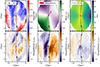 |
Fig. C.1. Disc stars (defined kinematically by vtoomre < 210 km s−1) binned in galactic X and Y. The top panels show the mean CDF of our vlos predictions (expected to be unbiased at 0.5), the mean vlos in the XY bin due to solar motion and the expected structure of the Disc, and the average uncertainty in our vlos prediction. The bottom panels show evidence of disequilibrium in the tangential, radial, and vertical velocity components of the stars, defined by the statistical significance of the deviation in the number of stars above or below the equilibrium values. The black arc and arrows show the local standard of motion. |
We see clear structures within our mean CDF values in the XY plane, indicating areas where our PDFs are systemically over and underestimating the vlos. This structure has no clear association with the number density of the sample or the binned mean vlos (middle panel). These trends are expected from a uniform Disc distribution and the Sun’s small relative velocity within the Disc, as indicated by the red arrow (in agreement with Naik24, Fig. 8). There is also no clear trend with distance. The third panel on the top row shows the mean σPDF binned in XY, which has little dependence on distance and is mainly dependent on the on sky position of the star, and it’s VTan.
Instead, we look at the dynamics within the Disc using the cylindrical components of velocity (vR, vϕ, vZ) (using the true RVS vlos values). We consider the deviation from expected equilibrium values to quantify disequilibrium in velocity. If the Disc is in phase-mixed equilibrium in every bin, we expect even numbers of stars moving up and down through the disc and in and out towards the centre of the Galaxy. Defining N+ and N− as the number of stars with a positive and negative velocity sign, respectively, we can estimate the statistical significance of any imbalance by modelling the distribution as a binomial, which can be approximated by a normal distribution. The statistical likelihood of getting (N+, N−) in units of sigma is then χ:
 (C.1)
(C.1)
where N is the total number of stars in the bin.
For the tangential component vϕ, we can define (N+, N−) as the number of stars in the bin above or below the median value of vϕ for stars at its given radius R, using a series of radial bins. In equilibrium, this should again be a binomial distribution, as there is an even probability that a star is above or below the median value. This quantity shows the deviation in the number of stars above or below the equilibrium values.
We plot these χ values for each of the velocity components in the bottom panels. They show strong, clear evidence for dynamical disequilibrium in Disc stars. The left panel showing the tangential value has very good agreement with the local spiral arm structure, as can be seen in Poggio et al. (2021) Fig. 5. The middle radial panel is consistent with Vislosky et al. (2024), and at the solar position, we are at the edge of a structure that is moving radially outward. The final panel of vertical motion shows a slight structure at a larger radius, away from the centre. There is more structure when comparing above and below the disc plane, which is likely linked to the Gaia phase space spiral (Antoja et al. 2018; Hunt et al. 2022).
These disequilibrium structures show correlations with our areas of under and over-predicting vlos, approximately matching the expected behaviour of seeing an excess in the median motion of stars. This effect is a small bias, and we do not expect to recover the disequilibrium structure.
Appendix D: Phase-clumped or phase-mixed
If we assume that all groups are phase-mixed, we find that the recovered velocity distributions are approximately evenly distributed between the signs of vZ and vR (see Fig. D.1). This methodology does not model the known 6D sample as effectively but makes fewer assumptions about the nature of the stellar groups. When modelling the true 5D Gaia dataset, it is important to consider the results of both methods to check for any new additional wraps or structures.
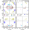 |
Fig. D.1. Cylindrical velocity distributions of the different stellar Halo groups, as recovered by our methodology (lefthand side), against the true distributions (righthand side). Different groups are represented using different colours, with the opacity of the colours indicating (0.5σ,1σ,2σ) levels (equivalently 38%,64%,95%). This figure is a comparison to Fig. 10, where the phase-clumped nature of the selected groups are additionally modelled with an additional step. Here are the results of assuming all groups are perfectly phase-mixed, resulting in near-symmetric velocity distributions in the radial and vertical components. |
All Figures
|
Fig. 1. Local sample of Gaia DR3 stars in different dynamical spaces (panels), classified into different groups (indicated by colour) by Dodd23. The panels show the spaces of energy and the vertical and perpendicular components of angular momentum used in Dodd23 to identify the Halo groups. The Disc group (purple) is kinematically selected with a Toomre velocity cut; the rest of the structures are found in the complementary kinematically selected Halo. In the plot, scatter points representing the Disc group have been down-sampled by a factor of 500, whilst the population in the legend is the total population of Disc stars. |
| In the text | |
|
Fig. 2. Our sample of 6D Gaia DR3 RVS stars in action space, classified into different groups of Dodd23 (indicated by colour). The Ungrouped Halo stars are represented by smoothed density, as indicated by the colours and contours in the colour bar. This density, and those of the individual groups, are corrected for selection effects (see text). Across the space is an example path (red line) of a 5D star through action space found by varying an assumed vlos, with values indicated in the legend. The corresponding PDF can be seen in the following Fig. 3. This example star is a GES member from the 6D Gaia RVS sample, with the true vlos and the corresponding point in action space marked by a square. |
| In the text | |
|
Fig. 3. PDFs of vlos, calculated from a 5D star’s path in action space (see Fig. 2). The thick black line total PDF shows the total density. This total can be decomposed into contributions from different groups, denoted by different colours. The probability that the star belongs to these different groups can be found by integrating the area under the respective lines, shown in the legend. As a star from the 6D sample, the true vlos is marked in green, and it is known that it is a GES member. Our method finds a 63% probability of belonging to GES but could also belong to Ungrouped Halo or Sequoia. |
| In the text | |
|
Fig. 4. Stars of un-phase-mixed groups in radial and vertical velocity space (in Galactic cylindrical coordinates). If the groups were phase-mixed, there would be a roughly equal number of stars from each group in every quadrant. Whilst not every group is in a single quadrant, none are consistent with being evenly distributed. |
| In the text | |
|
Fig. 5. Distributions of CDF values H(vTrue), calculated from the true vlos of the stars and the PDFs of our method, for each star in our Gaia RVS sample. If all assumptions and the PDFs are correct, these values should be distributed uniformly. We plot the total distribution of all stars and the distributions of the Disc and Halo stars (with CDF values corresponding to their respective PDFs). The total statistical error Δ% of our PDFs can be estimated by integrating the difference between the found and true uniform distribution. |
| In the text | |
|
Fig. 6. Distributions of σPDF (defined as half the 84%−16% vlos values) of the PDFs predicted by our method. The sample is split into Halo and Disc stars, whose normalised histograms of the true decomposition are plotted with solid-filled colours. The likely decomposition, defined by the probability of membership greater than 80%, is plotted with lines. The median values for the distributions for stars belonging to different groups (based on Dodd23) are shown in different colours. |
| In the text | |
|
Fig. 7. Distributions of the difference between vlos predictions and the true vlos across different subsamples of the Disc, the total Halo, and the stars belonging to substructure in the Halo. The top panel sample is from the Gaia RVS catalogue and includes vlos estimates our PDF’s the median and peak maximum values. The bottom panel shows a sample of stars from surveys crossmatched with Gaia and includes vlos estimates from Naik24. The tables contain the median velocity error for the different velocity predictions across the different subsamples. |
| In the text | |
|
Fig. 8. Uncertainty in our predicted vlos PDFs against the difference between the true value vTrue and our predicted line-of-sight velocity vmax. True Disc stars are plotted in purple, downsampled by a factor of 1000, the true Halo stars that are determined to be likely Halo stars by our method (probability greater than 80%) in orange, and true Halo stars that are misdetermined to be likely disc stars in red, both downsampled by a factor of 2. The median line and shaded regions indicate the binned running median and 1σ and 2σ values of the total distribution, defined from the 16%−84% range. If the predictions are unbiased and the predicted PDF uncertainties accurate, the binned 1σ and 2σ values regions are expected to follow the value of their own corresponding bin, plotted in solid black and blue lines. |
| In the text | |
|
Fig. 9. Distributions of various dynamical quantities of the Disc and Halo samples, defined kinematically by VToomre > 210 km s−1. The solid distributions are the original 6D distributions, and the lines are the recreated distributions from the 5D of the 6D sample by marginalising over the likely vlos PDFs inferred by our method. The top panel depicts the components of action space, and the bottom panel the components of velocity. |
| In the text | |
|
Fig. 10. Cylindrical velocity distributions of the different groups, as recovered by our methodology (lefthand side) against the true distributions (righthand side). Different stellar groups are represented by different colours, with the opacity of the colour representing the (0.5σ, 1σ, 2σ) levels (equivalently the 38%, 64%, and 95% regions). The groups are split into two separate subpanels, with the majority of phase-mixed groups in the top set and phase-clumped groups, with the addition of the Helmi Streams to allow the groups to be visually distinguished, in the bottom set. |
| In the text | |
|
Fig. 11. Distributions of membership probabilities of our individual groups (separate panels), calculated with our methodology. The distribution of the membership probabilities of every star is plotted in blue, and the true group members in orange. The first two panels depict the Disc and the total Halo. The total Halo is decomposed into individual structures and Ungrouped Halo. By construction, a star’s probabilities of belonging to the Disc or the total Halo sum to one, and the total Halo membership is then decomposed into belonging to structures or Ungrouped Halo. |
| In the text | |
|
Fig. 12. Expected populations of the stellar groups of our 6D RVS sample, calculated using membership probabilities assigned by our method, compared to the true population (based on Dodd23 groups). The error bars are estimated by redrawing the populations based on the membership probabilities of the stars. |
| In the text | |
|
Fig. 13. Plots depicting effects of increasing the minimum membership probability upon the purity and completeness of the selected sample of a group. For each group (panel), increasing the probability cut on membership probability (x-axis) increases the purity of the selected group, but decreases the completeness (y-axis). We plot the true purity and completeness, and the expected purity and completeness calculated from the probability distribution. For groups that show evidence of being phase-clumped, we also plot the purity and completeness calculated without the additional phase considerations (see Sect. 4.2). |
| In the text | |
|
Fig. 14. Curves describing the effective recovery for our different groupings, using the expected purity and completeness of a given probability cutoff. These curves describe the inherent trade-off of choosing a sample of stars; the higher the purity, the lower the completeness. Better recovered structures have a higher completeness for a given purity. In the first panel, we additionally plot the recovery curve from making a transverse sky velocity cut (see text for details). |
| In the text | |
|
Fig. 15. Comparisons between the differences between the true vlos and the predictions of our methodology and Naik24, with samples decomposed into different halo substructures. We include all stars from the true groups, plotted with triangles, and true likely members with membership probability greater than 50%. Only groups with more than 4 likely members are plotted. The points and error bars represent the median and the 16% and 84% percentiles of the distribution, respectively, for the likely groups. These results use the crossmatched 6D sample described in the main text. |
| In the text | |
|
Fig. 16. Plots of the dependence of Halo and Disc properties on VTan, the on sky velocity. The top panel shows the distribution of VTan against VToomre, where the horizontal red line depicts the VToomre cut used to kinematically define our Halo and Disc Samples. The middle panel shows the purity and completeness of the sample; for the common VTan > 200 km s−1 halo selection, the sample is 83% pure and 69% complete. The bottom panel shows the probability of the star belonging to the Disc, as inferred by our method. |
| In the text | |
|
Fig. 17. Stars from our ED-2 samples in R − z space, with velocities indicated as trails. In blue are the true known members from our 6D Gaia RVS sample. In orange, the likely members of ED-2 inferred from 5D information, without known vlos, by our method. The velocities are predicted from the most likely vlos corresponding to the peak of the PDF. In red, the stars were inferred without using the additional phase information of ED-2 (described in Sect. 4.2). Both of these samples have been selected with a minimum probability of pmin = 50%, corresponding to an expected purity of 86% with phase information and 56% when assuming the structure is phase-mixed. |
| In the text | |
|
Fig. C.1. Disc stars (defined kinematically by vtoomre < 210 km s−1) binned in galactic X and Y. The top panels show the mean CDF of our vlos predictions (expected to be unbiased at 0.5), the mean vlos in the XY bin due to solar motion and the expected structure of the Disc, and the average uncertainty in our vlos prediction. The bottom panels show evidence of disequilibrium in the tangential, radial, and vertical velocity components of the stars, defined by the statistical significance of the deviation in the number of stars above or below the equilibrium values. The black arc and arrows show the local standard of motion. |
| In the text | |
|
Fig. D.1. Cylindrical velocity distributions of the different stellar Halo groups, as recovered by our methodology (lefthand side), against the true distributions (righthand side). Different groups are represented using different colours, with the opacity of the colours indicating (0.5σ,1σ,2σ) levels (equivalently 38%,64%,95%). This figure is a comparison to Fig. 10, where the phase-clumped nature of the selected groups are additionally modelled with an additional step. Here are the results of assuming all groups are perfectly phase-mixed, resulting in near-symmetric velocity distributions in the radial and vertical components. |
| In the text | |
Current usage metrics show cumulative count of Article Views (full-text article views including HTML views, PDF and ePub downloads, according to the available data) and Abstracts Views on Vision4Press platform.
Data correspond to usage on the plateform after 2015. The current usage metrics is available 48-96 hours after online publication and is updated daily on week days.
Initial download of the metrics may take a while.