| Issue |
A&A
Volume 690, October 2024
|
|
|---|---|---|
| Article Number | A259 | |
| Number of page(s) | 21 | |
| Section | Extragalactic astronomy | |
| DOI | https://doi.org/10.1051/0004-6361/202349036 | |
| Published online | 15 October 2024 | |
SN 2021adxl: A luminous nearby interacting supernova in an extremely low-metallicity environment
1
The Oskar Klein Centre, Department of Astronomy, Stockholm University, AlbaNova, SE-10691 Stockholm, Sweden
2
Center for Interdisciplinary Exploration and Research in Astrophysics (CIERA), Northwestern University, 1800 Sherman Ave., Evanston, IL 60201, USA
3
The Oskar Klein Centre, Department of Physics, Stockholm University, AlbaNova, SE-10691 Stockholm, Sweden
4
Caltech Optical Observatories, California Institute of Technology, Pasadena, CA 91125, USA
5
Department of Particle Physics and Astrophysics, Weizmann Institute of Science, 234 Herzl St, 7610001 Rehovot, Israel
6
Graduate Institute of Astronomy, National Central University, 300 Jhongda Road, 32001 Jhongli, Taiwan
7
MIT-Kavli Institute for Astrophysics and Space Research, 77 Massachusetts Ave., Cambridge, MA 02139, USA
8
Department of Physics, Lancaster University, Lancaster LA1 4YW, UK
9
Astrophysics Research Institute, Liverpool John Moores University, IC2, Liverpool Science Park, 146 Brownlow Hill, Liverpool L3 5RF, UK
10
Division of Physics, Mathematics and Astronomy, California Institute of Technology, Pasadena, CA 91125, USA
11
IPAC, California Institute of Technology, 1200 E. California Blvd, Pasadena, CA 91125, USA
Received:
20
December
2023
Accepted:
18
June
2024
Abstract
SN 2021adxl is a slowly evolving, luminous, Type IIn supernova with asymmetric emission line profiles, similar to the well-studied SN 2010jl. We present extensive optical, near-ultraviolet, and near-infrared photometry and spectroscopy covering ∼1.5 years post discovery. SN 2021adxl occurred in an unusual environment, atop a vigorously star-forming region that is offset from its host galaxy core. The appearance of Lyα and O II, as well as the compact core, would classify the host of SN 2021adxl as a “Blueberry” galaxy, analogous to higher redshift, low-metallicity, star-forming dwarf “Green Pea” galaxies. Using several abundance indicators, we find a metallicity of the explosion environment of only ∼0.1 Z⊙, the lowest reported metallicity for a Type IIn SN environment. SN 2021adxl reaches a peak magnitude of Mr ≈ −20.2 mag and since discovery, SN 2021adxl has faded by only ∼4 magnitudes in the r band with a cumulative radiated energy of ∼1.5 × 1050 erg over 18 months. SN 2021adxl shows strong signs of interaction with a complex circumstellar medium, seen by the detection of X-rays, revealed by the detection of coronal emission lines, and through multi-component hydrogen and helium profiles. In order to further understand this interaction, we model the Hα profile using a Monte Carlo electron scattering code. The blueshifted high-velocity component is consistent with emission from a radially thin spherical shell resulting in the broad emission components due to electron scattering. Using the velocity evolution of this emitting shell, we find that the SN ejecta collide with circumstellar material of at least ∼5 M⊙ assuming a steady-state mass-loss rate of ∼4 − 6 × 10⁻³ M⊙ yr−1 for the first ∼200 days of evolution. SN 2021adxl was last observed to be slowly declining at ∼0.01 mag d−1, and if this trend continues, SN 2021adxl will remain observable after its current solar conjunction. Continuing the observations of SN 2021adxl may reveal signatures of dust formation or an infrared excess, similar to that seen for SN 2010jl.
Key words: circumstellar matter / supernovae: general / ISM: abundances / HII regions
Corresponding author; This email address is being protected from spambots. You need JavaScript enabled to view it.
© The Authors 2024
 Open Access article, published by EDP Sciences, under the terms of the Creative Commons Attribution License (https://creativecommons.org/licenses/by/4.0), which permits unrestricted use, distribution, and reproduction in any medium, provided the original work is properly cited.
This article is published in open access under the Subscribe to Open model. This email address is being protected from spambots. You need JavaScript enabled to view it. to support open access publication.
1. Introduction
Massive stars (> 8 M⊙) are expected to end their lives as core-collapse supernovae (CCSNe) (Woosley & Weaver 1995; Heger et al. 2003; Janka 2012; Crowther 2012). All-sky photometric surveys (Bellm 2014; Chambers et al. 2016; Tonry et al. 2018) are finding numerous supernovae (SNe) each night, but the exact mechanisms by which a massive star spends its final moments is currently unclear (see, e.g., Burrows & Vartanyan 2021). Supernovae that display narrow hydrogen emission lines atop a blue continuum are classified as Type IIn SNe (Schlegel 1990; Gal-Yam et al. 2007; Ransome et al. 2021). The narrow emission features are suggested to arise from the excitation of a slow-moving circumstellar medium (CSM) near the progenitor that has been photoionized by the ejecta-CSM interaction.
This CSM is expected to have been ejected by the progenitor in the years to decades before core collapse (Vink et al. 2008; Ofek et al. 2014). While a star ejects mass into the surrounding interstellar medium (ISM) throughout its life in the form of stellar winds with mass-loss rates of 10−7 − 10−4 M⊙ yr−1, studies of the progenitors of Type IIn SNe have reported much higher mass-loss rates of > 10−3 M⊙ yr−1 (Fransson et al. 2014; Moriya et al. 2014; Fraser 2020; Khatami & Kasen 2023). This likely reflects either eruptive mass-loss events, or enhanced steady-state mass loss by the progenitor in the decades prior to core-collapse.
The physical mechanism behind such an enhanced mass-loss rate is elusive, mainly due to the inability to directly observe these mass-loss events prior to supernova explosion. However, this brief period of enhanced mass loss likely influences the photometric evolution of the supernova, including duration and luminosity, as well as the spectroscopic appearance of emission or absorption line profiles and their evolution (see, e.g., Kurfürst & Krtička 2019; Suzuki et al. 2019, for the case of a disk–torus). These progenitors must have mass-loss rates not typically observed during the main sequence. It is suggested that the high mass-loss rates are similar to those of massive (> 25 M⊙) luminous blue variable (LBV) stars (e.g., Taddia et al. 2013; Weis & Bomans 2020) and some Type IIn SNe have been associated with such stars (e.g., SN 2005gl; Gal-Yam et al. 2007). Alternatively, Type IIn SNe may arise as a result of a superwind phase from a red super-giant (RSG) star (Fransson et al. 2002; Smith et al. 2009a). Current stellar evolution theory suggests that canonical LBVs are a short transitional phase, between a hydrogen-rich RSG evolving toward a hydrogen-depleted Wolf-Rayet (WR) star (Crowther 2007; Langer 2012; Ekström et al. 2012). The term LBV is typically employed to define a broad phenomenology rather than an evolutionary stage (e.g., Gal-Yam et al. 2007; Trundle et al. 2008; Dwarkadas 2011; Groh 2017). Standard stellar evolution theory predicts that single massive stars that become LBVs do so near the end of, or after, the completion of core hydrogen burning. Thereafter, they typically lose their hydrogen-rich envelopes in the LBV phase and become WR stars, where they spend ∼105 years, after which they explode as a CCSN.
To date, there is no clear understanding of how a star may undergo core-collapse at this phase (Chevalier 2012; Woosley 2017). However, under certain conditions, a progenitor may have the appearance of a LBV star shortly before core-collapse when the progenitor is rapidly rotating (e.g., Groh et al. 2013). In this scenario, the progenitor likely ejects the majority of its outer envelope during the RSG stage. It should be noted that these stars appear as LBV stars, but do not necessarily have the chemical composition of the canonical LBV (Humphreys & Davidson 1994; Weis & Bomans 2020). Studies of Type IIn SNe show a diverse range of peak magnitudes, ranging from −16 to −23 magnitudes (Nyholm et al. 2020; Ransome et al. 2021). Typically, SNe brighter than −21 mag are classified as superluminous supernovae (SLSNe) (Gal-Yam 2012, 2019), although for hydrogen-rich transients it is not clear if there is a defined boundary between regular SNe and SLSNe (of Type IIn) or rather an apparent continuity.
This paper presents a large dataset for SN 2021adxl that enables us to study the late-time evolution and environment of a nearby luminous Type IIn SN. An image of SN 2021adxl and its environment is given in Fig. 1. SN 2021adxl1 was discovered by the Zwicky Transient Factory (ZTF; Graham et al. 2019; Bellm et al. 2019; Dekany et al. 2020) at RA = 11:48:06.940, Dec = −12:38:41.71 (J2000) on 2021 November 08 at a r-band magnitude of 14.41 mag (Fremling 2021). SN 2021adxl was classified by De et al. 2022 on 2022 February 02 as a Type IIn SN at a redshift of z = 0.018 (reported wavelengths given in rest frame unless stated otherwise). The host of SN 2021adxl, WISEA J114806.88-123841.3, displays a unique morphology known in the literature as a tadpole galaxy (Elmegreen et al. 2012; Munoz-Tunon et al. 2014; Rosado-Belza et al. 2019), discussed further in Sect. 3. We assume a Hubble constant H0 = 73 km s−1 Mpc−1, ΩΛ = 0.73 and ΩM = 0.27 (Spergel et al. 2007). The corresponding luminosity distance DL = 78.16 Mpc and a distance modulus of μ = 34.47 ± 0.02 mag are used for SN 2021adxl. We correct for foreground extinction using RV = 3.1, E(B − V) = 0.026 and the extinction law given by Cardelli et al. (1989). Unless stated, we do not correct for any potential host galaxy or circumstellar extinction; however, we note that the blue colors seen in the spectra of SN 2021adxl, and in the host, do not point toward significant reddening by dust. Additionally, the lack of noticeable Na D λλ5890 5896 points toward low extinction, although a robust measurement cannot be made to do the strong He Iλ5876 emission. The rising part of the light curve of SN 2021adxl was not observed as the transient was discovered around its peak magnitude after ending solar conjunction. The rest-frame phase is taken with respect to the r-band discovery epoch on 2021 November 03 (MJD = 59521). Luminous SNe are intrinsically rare and are given the adopted distance of 78 Mpc. SN 2021adxl is the nearby Type IIn SN, and just as SN 2010jl (49 Mpc; Smith et al. 2011; Fransson et al. 2014; Ofek et al. 2014; Jencson et al. 2016), and due to its luminosity and slow evolution, it provides a rare opportunity to follow the evolution of such a transient for many years.
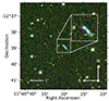 |
Fig. 1. P60/SEDM composite color image (gri) for SN 2021adxl (marked in the inset by the magenta crosshair) from the ZTF survey, when the transient was near peak. SN 2021adxl is contaminated by strong host emission, which can be seen in the inset. |
This paper is organized as follows. Section 2 provides details of the observational dataset presented in this paper, split into photometric data in Sect. 2.1 and spectroscopic data in Sect. 2.2. This section also gives an overview of the observable properties for SN 2021adxl. SN 2021adxl occurred in a bright star-forming region, and we discuss the host environment of SN 2021adxl in Sect. 3. A prominent feature of the optical spectra of SN 2021adxl is the broad Hα profile, and we explore the formation of this line in Sect. 4, as well as any insights into the ejecta-CSM interaction in Sect. 4. Finally in Sect. 5, using the results from observations, we investigate the metallicity of the host of SN 2021adxl and, in general, interacting SNe in Sect. 5.2, and we discuss the possible progenitor of SN 2021adxl in Sect. 5.3.
2. Observations
2.1. Photometry
Photometry in gri was obtained at the position of SN 2021adxl using the ZTF forced-photometry service2 (Masci et al. 2019). Quality checks were performed on the raw data and detections were chosen based on a signal-to-noise ratio (S/N) of S/N ≥ 3. Photometry from the ATLAS forced-photometry server3 (Tonry et al. 2018; Smith et al. 2020; Shingles et al. 2021) at the position of SN 2021adxl were obtained in the ATLAS c and o filters. We computed the weighted average of the fluxes of the observations on nightly cadence. We performed a quality cut of 3σ in the resulting flux of each night for both filters and then converted them to the AB magnitude system. A single epoch of photometry with the AAlhambra Faint Object Spectrograph and Camera, (ALFOSC) on the 2.56 m Nordic Optical Telescope (NOT) was obtained in gr and three epochs from the Liverpool Telescope (LT) with the optical imaging component of IO (Infrared-Optical) instrument was obtained in gri. J-band photometry was obtained with the Palomar Gattini-IR (PGIR) telescope shortly after SN 2021adxl was discovered and data were reduced following De et al. (2020). No significant activity/outbursts are detected in the pre-discovery images extending back to the beginning of the ZTF observing (circa 2018) to a limit of −14 mag. Our photometric dataset is given in Fig. 2 and photometric tables are available in the online material.
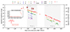 |
Fig. 2. Multi-band light curve of SN 2021adxl covering ∼1.6 years of its post-peak evolution. Highlighted in gray are two distinct phases where SN 2021adxl displays two distinct decline slopes, as mentioned in the text. The inset provides Gaia G-band data of SN 2021adxl (post-2022), as well as the historic observations of the explosion site (pre-2022, likely dominated by host flux). The right y-axis gives the apparent magnitude corrected for distance. Spectral epochs are given as vertical lines at the top of the plot. |
We observed the field SN 2021adxl with the Swift’s on board X-ray telescope XRT (Burrows et al. 2005) in photon-counting mode between 2022-02-23T16:47:35 (MJD: 59633.699) and 2022-04-16T12:19:33 (MJD: 59685.5136). We analyzed all photon-counting data with the online tools of the UK Swift team that use the methods described by Evans et al. (2007, 2009, 2020) and the software package HEAsoft4.
An image constructed from all XRT data reveals a fading source at RA, Dec (J2000) 11:48:06.72, −12:38:45.0 with an uncertainty of 5.3 arcsec (radius, 90% confidence), using the online tool of the UK Swift team5 (Evans et al. 2007, 2009). Using the dynamic binning method of the swift online tools, we obtain two detections summarized in Table 1. The number of counts is too low to robustly constrain the X-ray spectrum. To convert the count-rate to a flux, we assume an absorbed power law with a photon index of 2 where the absorption components is set to the Milky-Way value of  from HI4PI Collaboration (2016). Using these spectral parameters, we derive count rate to flux conversion factor of
  to infer the unabsorbed flux between 0.3 and 10 keV. The converted count rates are summarized in Table 1, and we discuss the X-ray luminosity further in Sect. 2.5.
XRT observations.
Due to its proximity at only 78 Mpc, and the fact that SN 2021adxl is a slow evolving luminous transient, fading by only 4.5 magnitudes during the 1.5 year (18 month) dataset presented in this work, this SN can potentially be followed-up for years. Figure 2 illustrates the entire multi-band observations of SN 2021adxl covering from discovery until solar conjunction in mid-2023. Spectroscopic follow-up began in February 2021, and is discussed further in Sect. 2.2.
The light curve of SN 2021adxl shows two distinct phases (referred to as Phase 1 and Phase 2) in its post-peak evolution. The peak itself is poorly sampled and it is unclear if Phase 1 extends to the earliest detections. Approximately 100 days post discovery, SN 2021adxl shows smooth decline of ∼0.6 mag/100 d, declining faster in the bluer bands, as is typical for Type IIn SNe (see Fig. 10 in Nyholm et al. 2020). After the mid-2022 solar conjunction, SN 2021adxl begins to decline at a slightly faster rate of 1 mag/100 d.
The rise to peak for SN 2021adxl was not observed due to solar conjunction in late-2021. An important aspect of Type IIn SNe is their rise time to maximum light, as there is a strong correlation between rise time and CSM/ejecta properties (e.g., Suzuki et al. 2016; Nyholm et al. 2020). The inset of Fig. 2 shows the Gaia G-band observations of the site of SN 2021adxl covering the past 9 years. Prior to SN 2021adxl, there is no significant variability seen at the explosion site. Similarity, no precursor signal is seen in forced-photometry measurements of ZTF, and ATLAS observations.
A pseudo-bolometric light curve is constructed using SUPERBOL6 (Nicholl 2018) from the photometry presented in Fig. 2, and calibrated using the extinction and distance given in Sect. 1. The resulting light curve is shown in Fig. 3. The bolometric light curve can be accurately characterized by a power-law decay from ∼0–300 days (with respect to discovery date), given by  and a final steep decay given as
  after ∼300 days. As shown in Fig. 3, this is similar to SN 2010jl (Fransson et al. 2014), but SN 2021adxl is around 66% less luminous.
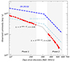 |
Fig. 3. Bolometric light curve for SN 2021adxl. The black dashed lines show power-law fits to the phase 1 and phase 2 light curves, with a distinct break at ∼+300 days post discovery. The dark blue dashed line is the similar power-law fit for SN 2010jl (Fransson et al. 2014), and the light blue line is the same fit scaled to match SN 2021adxl by eye. |
Figure 4 compares the r/R-band absolute light curve of SN 2021adxl with several transients with similar photometric appearance, most notably SN 2013L (Andrews et al. 2017; Taddia et al. 2020) and SN 2010jl (Fransson et al. 2014; Jencson et al. 2016). Additionally, Fig. 5 gives the extinction-corrected color evolution for each transient. Qualitatively, SN 2021adxl, SN 2013L, and SN 2010jl share the same light curve morphology and color evolution. Post peak, each of these transients light curves flattens after ∼100 days. SN 2021adxl shows a steeper decline compared to SN 2013L and SN 2010jl, with a slope similar to that seen in SN 2016aps (Nicholl et al. 2020), albeit ∼2 mags less luminous.
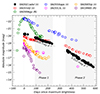 |
Fig. 4. r/R-band light curve comparison of luminous interacting SNe including SN 2021adxl. Each transient is corrected for distance and MW extinction. The regions labeled Phase 1 and Phase 2 correspond to the phases in the post-peak evolution where SN 2021adxl shows unique decline rates. |
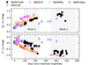 |
Fig. 5. Color comparison of bright Type IIn SNe including SN 2021adxl. Each transient has been corrected for MW extinction. |
After ∼250 days, SN 2021adxl begins to decline faster, and the same evolution is also clearly seen for SN 2010jl and SN 2013L, although with much poorer cadence for the latter. A similar trend was observed also for the Type IIn SN 2005ip; however, for that SN the first flattening stage happened later, at approximately +200 days (Stritzinger et al. 2012) and the second drop-off much later, at +3000 days (Fox et al. 2020). For contrast, the prototype Type IIn SN 1998S does not show any light-curve flattening, but declines rather quickly (Schlegel 1990; Mauerhan & Smith 2012).
As seen from Fig. 4, there is a spread in peak magnitudes for the transients. Under the assumption that the explosion mechanism for each transient is similar, for example core-collapse (Bethe 1990; Woosley & Weaver 1995; Smartt 2009) or pulsational-pair instabilities (Woosley 2017), the heterogeneity in brightness could be the result of different amounts of CSM or ejecta mass, although this assumes the explosion energy is similar for all Type IIns. We further discuss the ejecta and CSM properties of SN 2021adxl in Sect. 4
2.2. Spectral evolution
Figure 6 shows the earliest spectrum of SN 2021adxl, taken around the(apparent) peak brightness. Although the spectrum shows some undulations, its overall appearance is consistent with a Type IIn SN (i.e., a blue continuum with narrow hydrogen emission features) with underlying host flux seen in [O III] [O III] λ5007. SN 2021adxl was then classified as a Type IIn by De et al. 2022 using the Magellan/Baade with the FIRE NIR instrument on 2022 February 01 and the classification spectrum is shown in Fig. 7.
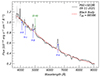 |
Fig. 6. Earliest spectrum of SN 2021adxl from P60/SEDM taken on 2021 November 09. The mean flux is given in black, with 1σ errors shaded in gray. |
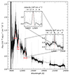 |
Fig. 7. Classification NIR spectrum of SN 2021adxl from the Magellan/FIRE from 2022 February 01 (De et al. 2022). A close-up of the Pa-β line is given in the inset on the right, with a zoomed-in profile in the upper left. The spectrum smoothed with a Savgol filter is given in black, with the raw data given in gray. |
Follow-up spectra were obtained using NOT/ALFOSC, the Low Resolution Imaging Spectrometer (LRIS; Oke et al. 1995) on the 10 m Keck telescope, the Double Spectrograph (DBSP) on the Palomar 200-inch telescope (P200), and the Spectral Energy Distribution Machine (SEDM; Blagorodnova et al. 2018; Rigault et al. 2019) on the Palomar 60-inch (P60) telescope. Observations using the P60 and P200 were coordinated using the FRITZ data platform (van der Walt et al. 2019; Coughlin et al. 2023). The spectra were reduced in a standard manner, using LPIPE (Perley 2019), DBSP_DRP (Mandigo-Stoba et al. 2022) and PYPEIT (Prochaska et al. 2020a,b,c), for Keck/LRIS, P200/DBSP, and NOT/ALFOSC, respectively, and SEDM spectra were reduced using the automated pipeline PYSEDM (Rigault et al. 2019; Kim et al. 2022).
A single UV spectrum was obtained using the Cosmic Origins Spectrograph (COS) on board the Hubble Space Telescope (HST) on 2022 April 11 (Program ID: 16931, PI: Yan) and is presented in Fig. 8. This spectrum was low S/N (upper panel of Fig. 8); however, when a smoothing filter is applied, we recover interstellar absorption bands (see Haser et al. 1998, and references therein), and several emission lines at the redshift of SN 2021adxl. Most features seen in the lower panel of Fig. 8 likely arise due to interstellar absorption within the MW, although we make tentative detections of N IV], O III], and He II, as well as Lyα, at the redshift of SN 2021adxl.
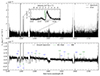 |
Fig. 8. HST/COS UV spectrum of SN 2021adxl taken with the G130M (FUV) and G160M (NUV) grism on 2022 April 11 (+158d). The upper panel shows the (error) spectrum given in (gray) black. The lower panel gives the science spectrum smoothed using a Savitzky–Golay (Savgol) filter with window size equal to 31 with a second-order polynomial. We include expected wavelengths for both Milky Way (MW) (in blue) and SN 2021adxl plus its host (in green), although the detection of some of these lines are unclear due to the low S/N of the science spectrum. |
A near UV spectrum was obtained on 2022 April 11 (Program ID: 16931, PI: Yan) using the Space Telescope Imaging Spectrograph (STIS) abroad HST and is presented in Fig. 9. The spectrum’s appearance does show some continuum flux, likely from SN 2021adxl, with a single broad feature at ∼ 2758 Å. While this may be broad/blended Mg IIλλ2796, 2803 (albeit offset by F ∼ 40 Å), it is also a possible a blend of several host/transient lines with superimposed interstellar lines, see inset of Fig. 9. The UV appearance of SN 2021adxl and its host is further discussed in Sect. 5.1.
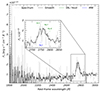 |
Fig. 9. HST/STIS with the G230LB grism on 2022 April 11 (+158d). The original science spectrum (gray) has been smoothed (black) using a Savgol filter with window size equal to 11 with a second-order polynomial. In the inset we show a close-up of the broad feature around 2759Å and include the expected wavelengths for both the interstellar (blue) and the SN 2021adxl (green) lines. |
We obtained four medium-resolution spectra with the X-shooter instrument (Vernet et al. 2011) between 2022 February 26 and 2023 February 2 (observing program 108.2262; PI. R. Lunnan). All observations were performed in nodding mode and with 1 0/0
0/0 9/0
9/0 9 wide slits (UVB/VIS/NIR). The first four epochs covered the full spectral range from 3000 to 24 800 Å. The integration times were varied between 2400 and 3700s. The data were reduced following Selsing et al. (2019). In brief, we first removed cosmic-rays with the tool ASTROSCRAPPY7, which is based on the cosmic-ray removal algorithm by van Dokkum (2001). Afterward, the data were processed with the X-shooter pipeline v3.3.5 and the ESO workflow engine ESOReflex (Goldoni et al. 2006; Modigliani et al. 2010). The UVB and VIS-arm data were reduced in stare mode to boost the S/N. In the background limited case, this can increase the S/N by a factor of
  compared to the standard nodding mode reduction (in the background limited case). The individual rectified, wavelength- and flux- calibrated two-dimensional spectra files were co-added using tools developed by J. Selsing8. The NIR data were reduced in nodding mode to ensure a good sky-line subtraction. In the third step, we extracted the one-dimensional spectra of each arm in a statistically optimal way using tools by J. Selsing. Finally, the wavelength calibration of all spectra were corrected for barycentric motion. The spectra of the individual arms were stitched by averaging the overlap regions. We note that to study the host galaxy, we reduced the data in nodding mode.
Figure 10 presents four epochs of spectroscopy taken with the VLT and the X-shooter medium-resolution spectrograph. All spectra were observed at parallactic angle with the UV, optical and IR regions stitched using a chi-2 minimization and flux calibrated top photometry taken on the same night. Two spectra were obtained during Phase 1 of the lightcurve, and two during Phase 2. The spectra show contributions from both transient light, seen by the broader emission profiles, as well as flux from the underlying host. At the time of writing, SN 2021adxl still dominates the flux at the location, and templates are currently unobtainable in order to remove narrow emission components from the host. All wavelength reports are given in rest-frame unless otherwise stated.
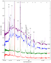 |
Fig. 10. VLT + X-shooter for SN 2021adxl taken at four different epochs. Each spectrum has been normalized with respect to Hα and offset for clarity. Emission lines expected from the transient (black) are denoted by the vertical lines. Telluric absorption bands arising from atmospheric O2 and H2O are denoted by the ⊕ symbol. We shade in regions of high noise levels from our first two spectra for visual clarity. |
2.3. Hydrogen spectral evolution
The most prominent and informative features in the spectra of Type IIn SNe is the Balmer series, and specifically the Hα profile (e.g., Roming et al. 2012; Ransome et al. 2021; Pursiainen et al. 2022). The Hα emission line has been used to constrain the progenitor wind velocity (Kankare et al. 2012; Andrews et al. 2017; Chugai 2019), explosion geometry (Hoffman et al. 2008; Andrews & Smith 2018; Pursiainen et al. 2022), and can potentially indicate late-time interaction (Silverman et al. 2013; Yan et al. 2015).
Type IIn SNe typically develop some asymmetries in their Hα emission line profiles in the post-peak evolution (Trundle et al. 2009; Fransson et al. 2014; Andrews et al. 2017, 2019; Moriya et al. 2020; Taddia et al. 2020; Pursiainen et al. 2022), and there are also cases where multiple absorption troughs are observed (Gutiérrez et al. 2017; Brennan et al. 2022). As noticed by De et al. (2022), the NIR classification spectrum for SN 2021adxl shows strong signs of hydrogen and helium emission. The insets of Fig. 7 give a close-up view of the Pa-β line, which is the best isolated hydrogen emission feature. In agreement with the initial classification, we resolve two apparent absorption features for the Pa-β line, one with a trough centered around ∼3500 km s−1 (right inset) and the second at ∼200 km s−1 (upper left inset). Although the latter has low S/N, a consistent absorption feature is seen also in other Paschen lines.
We observe a P Cygni profile at the approximate wavelength of Lyα in Fig. 8. The emission of Lyα is redshifted by ∼100 km s−1, with a blueshifted absorption centered at ∼ − 100 km s−1 (with respect to rest wavelength). Although the appearance of Lyα for SN 2021adxl is in contrast to the profile seen for SN 2010jl (Fransson et al. 2014), with SN 2021adxl showing a P Cygni profile, and SN 2010jl showing a purely absorption profile. This redshifted profile for SN 2021adxl may be a result of electron scattering (Huang & Chevalier 2018). As this spectrum is obtained ∼5 months post discovery, the P Cygni absorption likely originates from the pre-supernova stellar wind, located at large distances from the ejecta-CSM interface. This is consistent with the absorption seen earlier in Fig. 7. This would also suggest that SN 2021adxl has a very extended, dense circumstellar environment, which is likely correlated with the slow evolution observed in Fig. 2. However, we can speculate that the strange Lyα emission profile is a result of the host environment itself. We discuss this further in Sect. 3
Figure 11 highlights the evolution of the Hα profile from the VLT/X-shooter observations. The Hα profile consists of multiple distinct components, giving rise to an overall asymmetric appearance. A prominent blue-shifted emission component is observed in Hα and in other Balmer lines. This feature is not obviously seen in other emission features, for example in He I or Fe II, which suggests that the physical parameters forming this component are unique to a hydrogen-rich shell of material. This broad component does not extend to redder wavelengths, but the rather smooth line wings are indicative of electron scattering (Huang & Chevalier 2018). From the earliest X-shooter spectra, a third broad component can be resolved around rest wavelength with a superimposed narrow emission line likely arising from slow-moving CSM, an underlying H II region, or a combination of both.
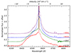 |
Fig. 11. Evolution of the Hα profile from the VLT/X-shooter observations. A pseudo-continuum has been removed from each profile, and the spectra normalized and offset for clarity. The phase given in gray (red) represents spectra obtained during (after) Phase 1. A noise spike at 6852Å was manually removed from the +115 d spectrum. |
As SN 2021adxl evolves, we see a smooth evolution of the Hα profile, most notably of the blueward component. The upper panel of Fig. 12 shows the complete optical spectral dataset (excluding the low-resolution P60+SEDM spectra). We mark the point where the flux of Hα exceeds 10% of the pseudo-continuum with a red cross. This component shows a smooth evolution during Phase 1, see lower panel of Fig. 12. During Phase 2 it is unclear if the Hα velocity continues to follow this trend as it apparently shows a quicker decline in velocity.
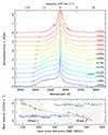 |
Fig. 12. Same as Fig. 11, but including the complete optical spectral dataset (excluding those from the P60/SEDM). A red cross in each profile denotes the maximum velocity of the blue excess for each spectrum. The lower panel gives the velocity of the bluest edge of the Hα profile, marked by the red cross in the upper panel. |
Compared to photometrically similar objects, SN 2021adxl shows qualitative similarities to the Type IIn SNe 2010jl (Fransson et al. 2014), 2013L (Andrews et al. 2017; Taddia et al. 2020) as well as SN 2005ip (Fox et al. 2020). Figure 13 compares the Hα profile of SN 2021adxl, SN 2010jl, and SN 2013L. Each transient shows a smooth redward wing, likely a result of electron scattering, as well as a blueward excess that evolves with time. It should be noted that while these three transients are qualitatively similar photometrically and spectroscopically, the photometric decline times and the emission line amplitude and offset are different among these events, and this may be due to differences in mass, velocity, and distribution of the emitting material. This might also be reflected in the different lightcurves, see Fig. 4. Insights can be gained by noting the +115d spectrum of SN 2021adxl compared to a spectrum of SN 2010jl at a similar epoch (+94d). SN 2021adxl shows flux out to 8000 km s−1 while SN 2010jl only shows a slight blue excess out to 2000 km s−1; however, this excess lines up quite well with the central wavelengths of the Hα profile at this time. Whereas the Hα profile of SN 2013L at this time matches the red wing of SN 2021adxl very well, and shows a much more dramatic flat-topped blue excess that persists for almost 4 years post peak (Andrews et al. 2017). Comparing the photometric evolution, SN 2013L shows a rapid decline before flattening, whereas SN 2010jl is more similar to SN 2021adxl, albeit declining at a slower rate.
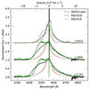 |
Fig. 13. Comparison of the Hα profile from SN 2021adxl, SN 2010jl (Fransson et al. 2014), and SN 2013L (Andrews et al. 2017; Taddia et al. 2020). Each transient shows a blue shoulder atop their respective Hα profile, as well as broad wings. Each profile has been normalized and offset for clarity. |
2.4. Helium spectral evolution
Aside from hydrogen, the spectrum of SN 2021adxl is dominated by strong Helium emission features, such as He Iλ4471, λ5876, λ7065 and λ10830, and possibly He Iλ2773 (see Fig. 9). In stark contrast to the Hα line, the profile of He Iλ5876 resembles a P Cygni profile. Figure 14 provides a cut-out around He Iλ5876, highlighting the strange P Cygni-like profile with an absorption feature at ∼4000 km s−1.
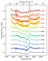 |
Fig. 14. Evolution of He Iλ5876 line. Each profile is continuum-subtracted. A double-Gaussian absorption profile is fitted to the blue side of each spectrum, and is given by the dashed black line. We do not attempt to include the components in emission, but the emission feature at rest wavelength narrows with time. |
Rather than the typical single absorption (e.g., Israelian & de Groot 1999), He Iλ5876 might show a second high-velocity (HV) feature, extending out to ∼18 000 km s−1. It is unclear whether this HV absorption is indeed associated with He I or a feature at bluer wavelength (e.g., the Na I D doublet λλ5890, 5896), which is blended with the He Iλ5876 line. If this is this case, a large amount of sodium-rich material must remain optically think more than 500 days post peak, and continue moving at very high velocities. In comparison to SN 2010jl, this double troughed absorption profile is not immediately obvious. In particular, the He Iλ5876 observed for SN 2010jl resembles the Hα profile (see, e.g., Fig. 2.5).
An alternative suggestion is that this HV material is associated with the He Iλ5876 line, although this feature is not clearly observed in other He I lines, due to severe line blending or telluric contamination, see Fig. 10. Seeing both absorption components would require an asymmetric explosion or CSM in order to see both the low- and high-velocity component, although maintaining a P Cygni -like absorption profile after 500 days is also difficult to explain.
2.5. X-ray emission from Interacting SNe
When the progenitor of SN 2021adxl exploded, a shock wave was formed due the collision of the fast moving ejecta and the slower moving CSM. X-ray emission, if detected, can be used to diagnose the shock wave interaction with the circumstellar medium (Chevalier & Fransson 2003; Dwarkadas 2019). We reported the detection of a decaying X-ray flux at the position of SN 2021adxl (see Table 1). This evolving X-ray is likely associated with SN 2021adxl and not the underlying source itself. We find the soft X-ray flux decreases from ∼3 × 1040 ergs s−1 at +113d to ∼0.9 × 1040 ergs s−1 at +160d. This flux is roughly a factor of 10 less than that found for SN 2010jl (Chandra et al. 2015). However, a meaningful comparison is moot due to the restricted X-ray cadence.
High-ionization lines have been observed in the optical spectra of nearby active galactic nuclei (AGNs) (Oke & Sargent 1968; Appenzeller & Oestreicher 1988; Lamperti et al. 2017); however, they are rarely observed in SNe (Turatto et al. 1993; Smith et al. 2009a), likely due to the lack of high- to medium-resolution spectra (Gröningsson et al. 2006; Komossa et al. 2009; Smith et al. 2009b; Pastorello et al. 2015; Fransson et al. 2014). These so-called “coronal lines”, first observed in the solar corona, arise from collisionally excited forbidden fine-structure transitions in highly ionized species such as Fe VI and Fe X.
Figure 15 shows our final X-shooter spectrum taken on 2023 February 26 with insets showing the location of several coronal emission lines. In terms of explosive transients, coronal lines have been interpreted in terms of dissipation of the energy of a shock wave in the circumstellar envelope. If collisional ionization is the dominant mechanism, then the presence of these lines implies a temperature of the emitting material of 105 − 106 K (Bryans et al. 2009) and pre-shock ionization of the circumstellar medium by X-ray emission. For SN 2021adxl, we do not detect [Fe XIV] λ5303 (see inset in Fig. 15), while [Fe X] λ6375 is strong meaning the CSM temperature is likely ≲2 × 10⁶ K (Jordan 1969; Turatto et al. 1993).
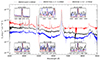 |
Fig. 15. Comparison of SN 2021adxl to the Type IIn SN 2010jl (Fransson et al. 2014), as well as the transitional Type Ic-BL/IIn SN 2017ens (Chen et al. 2018). The insets highlight the wavelength range around known coronal emission lines. Each inset has been normalized to the peak of each respective emission line. |
3. Host environment of SN 2021adxl
To further understand the host environment of SN 2021adxl, the software package PROSPECTOR version 1.1 (Johnson et al. 2021a) was used to analyze the spectral energy distribution from the host.
We retrieved science-ready coadded images from the Galaxy Evolution Explorer (GALEX) general release 6/7 (Martin et al. 2005), the Panoramic Survey Telescope and Rapid Response System (Pan-STARRS, PS1) DR1 (Chambers et al. 2016) and images from the Wide-Field Infrared Survey Explorer (WISE; Wright et al. 2010) processed by Lang (2014). We measured the brightness of the host using the Lambda Adaptive Multi-Band Deblending Algorithm in R (LAMBDAR9) (Lambda Adaptive Multi-Band Deblending Algorithm in R; Wright et al. 2016) and the methods described in Schulze et al. (2021). We also extract the photometry of the isolated star-forming region, in which the SN occurred. Table 2 the measurements in the different bands, and Table 3 focuses on the bright star-forming knot.
Photometric measurements of the host of SN 2021adxl.
Photometry of the isolated star-forming region where SN 2021adxl exploded.
We model the observed spectral energy distribution (black data points in Figure 16) with the software package PROSPECTOR version 1.1 (Johnson et al. 2021a).10 We assume a Chabrier IMF (Chabrier 2003) and approximate the star formation history (SFH) by a linearly increasing SFH at early times followed by an exponential decline at late times [functional form t × exp(−t/τ), where t is the age of the SFH episode and τ is the e-folding timescale]. The model is attenuated with the Calzetti et al. (2000) model. The priors of the model parameters are set identically to those used by Schulze et al. (2021). Figure 16 shows the observed SED (black data points) and its best fit (gray curve). The SED is adequately described by a galaxy template with a log mass of  , a star formation rate of
  . The mass and the star formation rate are comparable to common star-forming galaxies of that stellar mass (gray band in Figure 17; Elbaz et al. 2007), and they are also similar to those of the host galaxy populations of SNe IIn and SLSNe-IIn from the PTF survey (Schulze et al. 2021) albeit in the lower half of the mass distribution. In the same figure, we also show the location of the star-forming knot where the SN exploded in a lighter shade. This region has a somewhat lower specific star-formation rate (i.e., star formation rate normalized by galaxy mass) than of the entire galaxy but consistent within errors.
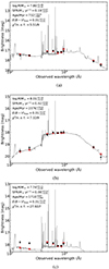 |
Fig. 16. Spectral energy distribution of the host galaxy from 1000 to 60 000 Å (black dots). The solid line displays the best fitting model of the SED. The red squares represent the model-predicted magnitudes. The fitting parameters are shown in the upper left corner. The abbreviation ‘n.o.f.’ stands for the number of filters. We performed measurements on the entire host flux (upper panel), the faint tail (middle panel), and the star-forming blob (lower panel) where SN 2021adxl exploded. (a) Flux from the host, including the flux from the bright head and the ffuse tail. (b) Flux from diffuse tail to the southwest. (c) Flux from bright star-forming head to the northwest. |
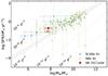 |
Fig. 17. Star formation rate and stellar mass of the host galaxy of SN 2021adxl (dark red) and of the bright star-forming region where the SN exploded (pink) in the context of SN-IIn and SLSN-IIn host galaxies from the PTF survey (Schulze et al. 2021). The host galaxy of SN 2021adxl lies in the expected parameter space of SN-IIn and SLSN-IIn host galaxies, but in the lower half of the mass and SFR distributions. Its specific star formation rate (SFR/mass) is slightly higher than the typical star-forming galaxies (gray band), but lower than for an average SLSN host galaxy. |
We focus on the narrow emission lines and the auroral emission lines associated with the underlying host (see review by Kewley et al. 2019, and references therein). The final X-shooter spectrum is utilized due to its long exposure time, and therefore higher S/N, although many of these diagnostic lines are present in all X-shooter spectra. As seen in Fig. 18, the late-time X-shooter spectra contain numerous narrow emission lines that are typically associated with H II regions. These narrow lines can provide insight into the metallicity (Z), the amount of dust, the electron temperature (Te) and density (ne), the age of the nebula, and the rate of star formation. However, transient flux is still clearly present in our latest X-shooter spectrum. We extract a trace in the 2D spectrum from a region offset from SN 2021adxl in order to minimize the contamination from SN 2021adxl, while still detected weak lines needed for abundance measurements, given in Fig. 19. A single narrow Gaussian emission line is fitted to each emission feature, while simultaneously fitting a pseudo-continuum. This offset spectrum still displays a weak offset broad component seen in Hα, so the following measurements (i.e., those that rely on hydrogen emission lines) may be slightly overestimated due to transient contamination. Investigating the Balmer decrement, we find Hα/Hβ ≈ 2.5 ± 0.2 and Hγ/Hβ ≈ 0.47 ± 0.07, consistent with negligible interstellar reddening, as would be expected form the blue appearance of the surrounding environment, see Figs. 20 and 21.
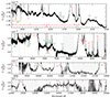 |
Fig. 18. VLT/X-shooter for SN 2021adxl taken on 2023 February 26 (+480d). The spectrum has been fluxed calibrated to the r-band and each panel highlights a wavelength range that (roughly) covers the near UV, optical, and near-IR. The telluric bands are marked by the gray area. The bottom two panels have been smoothed using a Savgol filter for clarity. |
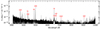 |
Fig. 19. Spectrum extracted from a region offset from the X-shooter spectrum taken on 2023 February 26. Emission lines used in metallicity, Te, and ne measurements are marked in red. Transient flux is still present in the spectrum, as is seen by the broad appearance of Hα and Hβ. |
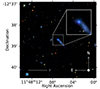 |
Fig. 20. Composite (gri) color image of the host galaxy of SN 2021adxl obtained from the DESI Legacy Surveys (Dey et al. 2019). SN 2021adxl (not visible in this image) exploded in the northeast part of its host, in a bright star-forming area. The inset provides a zoomed-in image of the explosion site, where the position of SN 2021adxl is marked by the crosshair. |
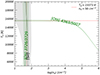 |
Fig. 21. A 4″ × 4″ cutout from the HST/STIS acquisition images from 2022 April 11 (+159 d) including SN 2021adxl as well as the compact bright star-forming knot. SN 2021adxl is separated from this compact knot by roughly half an arcsecond, or a projected distance of ∼0.2 kpc. |
We measure values for Te and ne using PYNEB11 (Luridiana et al. 2014) using [O III] λ4363/λ5007 as a temperature sensitive probe, and [O II] λ3726/λ3729, and [S II] λ6731/λ6716 as density-sensitive probes, see Fig. 22. Encouragingly, we find similar results as for the abundance indicators above with Te ≈ 16 000 K, ne ≈ 55 cm−3. Using [O II] and [O III], we can constrain Te and ne well, whereas the ne is not well constrained by [S II], again likely due to the low-density environment limit of 1.5 (Osterbrock & Ferland 2006). We search for other features to use within PYNEB, but found no other significant diagnostic lines. These may be due to the high-ionizing host flux, inhibiting these emission lines, or due to the low inferred densities. Using PYNEB, we find a metallicity of 12 + log((O+ + O++/H) = 7.61 dex (0.08 Z⊙), taking the solar value to be  dex (Asplund et al. 2021) and assuming the O II temperature dependence from Stasińska (1982).
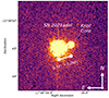 |
Fig. 22. Emission-line temperature and density diagnostic plot from PYNEB using [O III] λ4363/λ5007 as a temperature sensitive probe, and [O II] λ3726/λ3729 and [S II] λ6731/λ6716 as density-sensitive probes. |
To compare the explosion site with those of other SNe IIn, we also investigate abundance indicators using the narrow Hα and Hβ components, such as the commonly adopted N2 and O3N2 techniques (Pettini & Pagel 2004). These methods use the [N II] λ 6583 emission line which is detected in our +480d X-shooter spectrum, but has a low S/N ≲ 5, and has complex underlying flux, due to the broad Hα profile. Although there is some scatter in the derived metallicities, all methods strongly point toward a very low-metallicity environment of 0.05 − 0.2 Z⊙.
Tables A.2 and A.3 give the results from the various abundance methods to determine the metallicity of the underlying environment around SN 2021adxl. Similar results (i.e., low metallicity) are found using the transient dominated spectrum from 2023 February 26 (e.g., Fig. 18), although to irrefutably confirm the metallicity of the host, we require late-time spectral templates once SN 2021adxl has faded.
4. Modeling the Hα profile
In order to understand the formation of the hydrogen emission lines, we note two distinct features, one is the offset flat topped emission profile, which suggests of a thin emitting shell (Jerkstrand 2017) and the second is the red-ward, extended wings, which are characteristic of electron scattering (Huang & Chevalier 2018).
The collision of the fast moving ejecta with the slower moving CSM results in the formation of a dense shell of material. This shell is made up of swept-up, shock-heated gas from the circumstellar medium and can efficiently cool to relatively low temperatures compared to the high-energy, shock-heated gas found in other parts of the supernova ejecta. This cool dense shell (CDS) of material is bound between the outward moving forward shock and receding reverse shock (Chugai et al. 2004; Smith 2017a). Diffusion of radiation from this shocked shell produces the main continuum (e.g., red line in Fig. 6) as well as the intermediate (∼103 km s−1) components of Hα.
Under the assumption that the Hα profile arises from photons emitted from the CDS that undergo multiple scattering events as they travel outward through the surrounding media, a model of electron scattering is explored. A Monte Carlo code was developed12 in order to follow photons emitted from a thin shell as they travel through a diffuse medium. The code is based on the work by Pozdnyakov et al. (1983) and similar codes have been employed in previous works on interacting SNe (e.g., Fransson et al. 2014; Taddia et al. 2020). In this model, photons are emitted with an emissivity η, which varies with the electron density as ∝ne2 and ne ∝ r−2. Photons are followed until they escape the scattering medium, with a probability ∝e−τe. We include an occulting photosphere, meaning that any escaping photons moving away from the observer are excluded. The optical depth, electron temperature, and radius are degenerate in these electron scattering models (see Huang & Chevalier 2018, for details), and are left as restricted parameters. While this is nonphysical for a SN explosion as these parameters evolve with time, the models can be used to understand the formation of the Hα profile, as well as to further understand the main properties of the SN and, in particular, the shock velocity (Vshock) and mass-loss rate (Ṁ).
Figure 23 shows the first epoch X-shooter spectrum with the best fitting electron scattering model. The model matches the spectrum well, capturing the blue shoulder as well as the extended red wing. However, the model fails to capture the features around rest wavelength. This likely represents emission from slowly moving material surrounding the SN ejecta, as well as emission from the host.
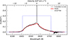 |
Fig. 23. Hα profile from the VLT/X-shooter spectrum (black) with the best fitting electron scattering model (red) for a given input spectrum (blue). The model matches the blue and red sides of the emission line well, but leaves an intermediate and narrow emission component at the central wavelength. |
Similar to Fig. 23, Fig. 24 shows the best fitting model for the earliest X-shooter spectrum, but with additional two Gaussian components, which likely reflect emission from the host and from CSM material far away from the shock (which we do not include in our models). As demonstrated in Fig. 12, the Hα profile evolves with time, and most notably, its blueward component moves toward the central wavelength. Using a grid of electron scattering models with an input spectrum representing a thin emitting shell, we are able to match the best fit model to the Hα profile for each spectrum (excluding the SEDM spectra due to their low resolution) to better understand how this blueward feature evolves. Figure 25 gives the results of the evolution of the velocity needed to produce the Hα profile at each epoch. During Phase 1, the velocity evolution is well fitted by
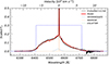 |
Fig. 24. Same as Fig. 23, but now including an additional intermediate and narrow Gaussian emission component. These three components can reproduce the entire Hα profile well. |
![Mathematical equation: $$ \begin{aligned} {V_{\rm shock}} = 6625 \times \left[ \frac{t}{100\,\mathrm {days}} \right] ^{-0.37} \,\mathrm {km\,s^{-1}}. \end{aligned} $$](/articles/aa/full_html/2024/10/aa49036-23/aa49036-23-eq16.gif) (1)
(1)
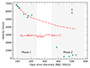 |
Fig. 25. Input velocities of the best fitting models needed to fit the Hα profile evolution. Velocities during Phase 1 are fitted with an exponential decline, given in red. During Phase 2, the velocities are lower and no longer follow the trend seen in Phase 1. This is likely due to the forward shock becoming optically thin, which is also seen in the faster decay rate in the bolometric light curve seen in Fig. 4. The error bar in the upper right denotes the velocity grid-resolution of the input spectra. |
At the beginning of Phase 2, the model velocities are much lower and no longer follow Eq. (1). Models fitted in Phase 2 show more scatter in their inferred velocity, and one should note the additional complexity of the Hα profile at this time as shown in Fig. 12.
The dominating energy input during the evolution of Type IIn SNe is due to the interaction between the SN ejecta and the surrounding CSM (Dessart et al. 2015). The diversity of the mass, velocities, and geometry of this interacting material are likely responsible for the heterogeneous appearance of this subclass (Chatzopoulos et al. 2012; Nyholm et al. 2020; Khatami & Kasen 2023). The total luminosity generated by ejecta-CSM interaction can be high because a radiative shock is a very efficient engine to convert kinetic energy into radiation at optical wavelengths. The luminosity of the CSM interaction is dependent on the velocity at which CSM enters the forward shock and on the progenitor’s mass-loss rate (Ṁ), and is typically given by
 (2)
(2)
assuming a steady mass-loss rate for the CSM (Wood-Vasey et al. 2004) and a 50% conversion efficiency (ϵ = 0.5). It is often difficult to determine the shock velocity from the line profiles given the uncertainty to which extent electron scattering plays a role in determining the widths of the intermediate lines (see discussion by Smith 2017a). SN 2021adxl offers a unique test to measure the degree to which electron scattering plays a role, as discussed in Sect. 4, and therefore to gain insight into the ejecta-CSM interaction.
Using Eqs. (1) and (2), we fit the Phase 1 portion of the light curve with the mass-loss rate Ṁ as a free parameter. The CSM velocity is taken to be ∼250 km s−1, as seen in the earliest spectrum, see Fig. 7, as well as the HST/COS spectrum given, see Fig. 8. As discussed in Sect. 4, the blue component of the Hα profile is likely caused by line scattering from a somewhat optically thin CDS. One interpretation of this is that photons are emitted from the outer regions of the CDS, and while travelling radially outward, scatter off material swept up by the forward shock.
It is important to note that the measurements of the shock velocity as provided in Eq. (1) are not based on the photometric evolution, but rather model fitting of the Hα profile. The exponent for the shock velocity evolution in Eq. (2) is responsible for the slope, and it is encouraging that the resulting fit in Fig. 26 matches the bolometric evolution so well. Equations (1) and (2) fits the luminosity of Phase 1 but this does not extend to Phase 2, where a faster, apparently linear, decline is seen. Extrapolating both trends, we expect a break around +300 d. Following Eq. (2), a steady-state mass-loss rate of 4 − 6 × 10⁻³ M⊙ yr−1 is required to provide the necessary luminosity if powered solely by shock interaction. Additionally, it is possible to fit a second decline (similar to Eq. (2)) to Phase 2 with a quicker velocity decline with an exponent of ≈ − 1.3; however, it is difficult to constrain this.
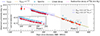 |
Fig. 26. Pseudo-bolometric light curve of SN 2021adxl. The best fitting model from Eq. (2) fitting to Phase 1 photometry (spectra) is given as the solid (dashed) blue line. Included in the inset is a zoomed-in image of this phase. Both a linear decline (dashed green) and possible shock luminosity curve (solid orange) is fitted to Phase 2. The magenta line is the decay expected for radioactive nickel, fitted to Phase 2, as discussed in Sect. 4. |
The use of Eq. (2) is likely an oversimplification but provides an estimate to the mass-loss rate from the progenitor shortly before the SN explosion. A mass-loss rate of 10−3 M⊙ yr−1 is consistent with reported values for other interacting SNe (Taddia et al. 2013; Ofek et al. 2014; Fransson et al. 2014; Moriya et al. 2014, 2023) as well as the values often assumed for Luminous Blue Variable (LBV) progenitors (Trundle et al. 2008; Dwarkadas 2011; Groh et al. 2013; Smith 2017b; Weis & Bomans 2020) as discussed further in Sect. 5.3.
As shown in Fig. 2, SN 2021adxl undergoes a steeper decline after Phase 1 and the trend seen in Fig. 25 may be related, perhaps reflecting a change in CSM density, distribution, or opacities, (see, e.g., discussion for SN 2010jl in Ofek et al. 2014; Moriya 2014). This is also observed in the evolution of the Hα profile in Fig. 12, when the overall profile narrows during Phase 2, likely reflecting a lower optical depth for material ahead of the shock from, meaning fewer scattering events (Huang & Chevalier 2018) and less broadening of the emission profile.
If we assume the ejecta-CSM interaction ceases when the shock reaches the edge of the dense CSM at a time tend, we can estimate the radial extent of this material (dCSM) using
 (3)
(3)
where tstart is the time at which the SN ejecta collides with the CSM, launching the forward shock into the dense CSM, and we use Vshock(t) from Eq. (1). We do not have a constraint on the explosion date so we cannot be certain on the duration of CSM interaction.
We make an conservative estimation of dCSM by assuming that tstart = 100 days, tend = 300 days and tduration ≈ 200 days (although this value may be a factor of 2 or more greater), the timeframe for which Eq. (1) is likely to be valid (i.e., the duration of Phase 1). This gives an approximate size of dCSM of 8 × 1017 cm (this is more than an order of magnitude larger that that reported for SN 2010jl for example Dwek et al. 2021) meaning that the CSM travelling at ∼250 km s−1 would have been ejected in the last ∼1000 years. We can set a lower limit on the CSM mass in Phase 1, assuming a constant Ṁ = 4 × 10⁻³ M⊙ yr−1, homologous distribution, and spherical symmetry, as MCSM ⪆ 4.3 M⊙. Additionally this mass will be substantially higher if we have overestimated Vwind or underestimated tstart and tend, although this is hard to quantify as we are uncertain how Vshock evolves for t ≲ 100 days. This high CSM mass is similar to that measured for SN 2010jl (∼1 − 10 M⊙; Zhang et al. 2012; Fransson et al. 2014; Ofek et al. 2014) and is likely a contributing reason for the slow evolution seen in both transients.
Assuming SN 2021adxl to be entirely powered by radioactive decay, Fig. 26 includes the energy deposited by a mass of explosively synthesized radioactive material given by Jeffery (1999), and the mass of radioactive nickel needed would be on the order of 3-10 M⊙ of material. However, such a mass of nickel would produce a much brighter transient, and would overpredict the luminosity evolution during Phase 1. This is obviously an overestimate, and not expected for SN 2021adxl, as the transient is likely dominated by CSM interaction even in Phase 2. We conclude that CSM interaction likely dominates Phase 2, although there is a different CSM mass/distribution when compared to Phase 1 meaning the progenitor has undergone several mass-loss episodes in the final moments before core-collapse.
5. Discussion
SN 2021adxl is an example of a nearby, bright, long-lasting interacting supernova. This allows a rare glimpse into the late-time evolution of the transient, and for this purpose we have obtained high-resolution spectra. Figure 18 provides a detailed picture of the final VLT/X-shooter spectrum taken at +480d. This highlights the weaker, narrow emission features that are typically missed when lower-resolution spectrographs are employed. For context, many narrow features discussed in this section are not detected in the NOT/ALFOSC spectra. This suggests an inefficient observing strategy for late-time transient followup when only low-medium spectrum are obtained.
5.1. The nature of the SN 2021adxl’s host
The Lyα profile seen in Fig. 8 is in contrast to the appearance of Hα as shown in Fig. 11. While this may be an opacity effect, or possibly due to emission from material far away from the ejecta-CSM interface as mentioned above, similar profiles for Lyα have been seen for population of compact, star-forming galaxies at z ∼ 0.2–0.3, also known as “green peas” (GP) galaxies (Cardamone et al. 2009). These GP galaxies have a high [O III] λ 5007/[O II] λ 3726 ratio, high equivalent width in O III emission lines (see Table A.2 Cardamone et al. 2009), and are typically subsolar metallicity (Orlitová et al. 2018; Liu et al. 2022). Our PROSPECTOR measurements also find a mass consistent with GP (∼108 M⊙; Cardamone et al. 2009). Although due to its proximity, the host of SN 2021adxl would be classified as a Blueberry galaxy rather than a Green Pea (Liu et al. 2022).
As shown in Fig. 8, the Lyα shows a unique profile that is not clearly seen in any other emission profile. The profile may resemble a P Cygni emission profile, typically observed in stellar winds and SNe, or a doubled peaked emission profile with an absorption trough at center wavelength. We note the similarities of the HST/STIS Lyα profile to that observed in GP galaxies (e.g., Yang et al. 2016; Orlitová et al. 2018; Henry et al. 2018). In this case, the asymmetric profile is thought to be due to resonant scattering of Lyα photons off neutral hydrogen atoms, which is dependant on the intervening material and fraction of escaping ionizing radiation. This would also point that the broad feature in Fig. 9 would be Mg IIλλ2796, 2803 (Henry et al. 2018), originating from the host and not SN 2021adxl, although does not explain the observed wavelength offset.
5.2. Type IIn SNe exploding in metal-poor environments
Perhaps greater insight may be gained from the local environment around SN 2021adxl. As mentioned in Sect. 3, SN 2021adxl occurred in a bright star-forming region at the end of an elongated intensity distribution. We find that the local environment has a very low metallicity of 0.06 Z⊙. This is similar to the environments for SN 2010jl (Stoll et al. 2011) and SN 2013L (Taddia et al. 2020), as well as for other Type IIn SNe (Habergham et al. 2014; Moriya et al. 2023).
Figure 27 compares the measured metallicities for the host of SN 2021adxl to a sample of values for hosts of Type IIn SNe (Habergham et al. 2014; Moriya et al. 2023), Type II SLSN (Leloudas et al. 2015), as well as both Type I and II SLSNe (Perley et al. 2016). SN 2021adxl is at drastically lower metallicity than the sample of Type IIn SNe (e.g., samples from Habergham et al. 2014; Moriya et al. 2023), and also lower that for Type II SN hosts (except perhaps for SN 2015bs; Anderson et al. 2016, 2018). The sample of Moriya et al. 2023 does include SN 2016iaf having 12 + log(O/H) = 7.48 ± 0.81 using the D16 method (Dopita et al. 2016), although this metallicity is outside the reported validity range for D16.
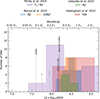 |
Fig. 27. Metallicity measurements for the environment around SN 2021adxl using the VLT/X-shooter spectrum on 2023 February 26 (+480d). The histograms are measured metallicities for hosts of Type IIn SNe (Habergham et al. 2014; Moriya et al. 2023), Type II SLSNe (Leloudas et al. 2015), and both Type I and II SLSNe (Perley et al. 2016) using various methods, denoted in the legend, and detailed in Sect. 3. The vertical lines mark measured values for SN 2021adxl using different methods (see text). We also mark the reported metallicity for SN 2010jl at Z ≈ 0.32 Z⊙ (Stoll et al. 2011) and for SN 2013L at Z ≈ 0.30 Z⊙ (Taddia et al. 2020). |
Moriya et al. (2023) find that Type IIn SNe with a higher peak luminosity occur in environments with lower metallicity and young stellar environment. Although SN 2021adxl is beyond the range explored by Moriya et al. (2023), the location and metallicity of the environment SN 2021adxl occurred in may explain its brightness. The conjecture that more luminous IIn’s are found in less metal-rich environments is in conflict with results from Leloudas et al. (2015), Perley et al. (2016) and Schulze et al. (2018, 2021). Figure 27 is contradicting this scenario, too. The SLSN-II sample spans the full range of metallicities (e.g., sample from Leloudas et al. 2015, in Fig. 27). The fact that they are super-luminous, and therefore more luminous than SN 2021adxl implies that their environments should on average be less metal enriched than of SN 2021adxl, in contradiction with the result of Moriya et al. (2023). Additionally, Moriya et al. (2023) find a strong inverse correlation between peak luminosity and metallicity, which may possibly explain the brightness of SN 2021adxl although the peak magnitude would be overestimated by almost 2 magnitudes (see Fig. 1 of Moriya et al. 2023).
5.3. Progenitor of SN 2021adxl
A major problem in supernova science concerns identifying the progenitors of Type IIn SNe. Progress is further hindered by the lack of clear nebular emission line signatures (which may reveal clues to the progenitor; e.g., Fraser et al. 2013; Jerkstrand et al. 2020). We are therefore often left with modeling the light curve and spectra, which in the case of interacting transients, are dominated by the effects of interaction, obscuring the signatures of any explosion mechanism (Arcavi et al. 2017; Woosley 2018).
There are no progenitor detections of SN 2021adxl, so we must rely on indirect methods. In Sect. 4, we concluded that SN 2021adxl can be powered by the ejecta colliding with a previous wind with Ṁ ≈ 10−3 M⊙ yr−1. This mass-loss rate regime is often reserved for LBVs during their outburst stages (Lamers 1989; Weis 2001; Vink 2008; Smith 2013), and additionally the inferred wind velocity is also similar to that observed among Galactic LBVs (Weis 2001).
Such high mass-loss rates are commonly inferred for Type IIn SNe (Moriya et al. 2014), although it is difficult to have a physical mechanism that can lead to this amount of mass ejected (Fuller 2017; Tsang et al. 2022). Such a high steady-state mass-loss rate is unlikely to be obtained from a single star. Using Eq. (20) from Björklund et al. (2021), a massive hot star would require a luminosity of L ≈ 107.2 L⊙ to achieve a steady-state mass-loss rate of 10−3 M⊙ yr−1 at a metallicity of 0.2 Z⊙ (this is the lower validity range from Björklund et al. 2021), which would likely exceed the Eddington luminosity of a single star. This is similar to the luminosity expected from the 1840 Giant Eruption of Eta Carinae (Davidson & Humphreys 2012), where it is thought that binary interaction was the cause of the eruption (see Smith 2011, for a possible scenario).
The involvement of a companion in the progenitor history is an often explored formation channel for Type IIn SNe (Chatzopoulos et al. 2012; Justham et al. 2014; Zapartas et al. 2019), as most massive stars are expected to be born and interact with a binary companion (Sana et al. 2012; Zapartas et al. 2019). The environments of Type IIn do not show dramatic differences when compared to normal Type II (Kelly & Kirshner 2012), suggesting there is no significant environment dependence for these two subtypes, and (possibly) they are influenced by the present (or absence) of a companion. At the time of writing SN 2021adxl no obvious signatures of binarity (e.g., pre-explosion variability, multi-peaked emission lines) are detected. While SN 2021adxl is a luminous Type IIn supernova, it does not reach the often assumed −21 mag criteria of SLSNe (Gal-Yam 2012). However, in the context of interacting SNe, it is not clear whether SNe IIn fulfilling this criterion constitute a separate population of events (Moriya et al. 2018; Gal-Yam 2019; Nyholm et al. 2020) or whether there is a continuum of possible energetics (see Fig. 1 of Moriya et al. 2023).
6. Conclusions
We present 1.5 years of the evolution of the luminous Type IIn SN 2021adxl, including four epochs of the spectra from the VLT/X-shooter. SN 2021adxl, similar to SN 2010jl, does not evolve quickly, and discovery has only faded by ∼4 magnitudes. This likely reflects that the forward shock, created from the ejecta–CSM interaction, is moving outward through a dense, extended CSM environment. The effects of this environment are seen in the appearance of the Hα emission line, which displays a persistent blue shoulder emission component. We find that this feature is due to electron scattering through an increasingly diffuse medium ahead of the forward shock. Using the evolution of this feature, we find that the post-peak evolution is dominated by the ejecta-CSM interaction. Assuming spherical symmetry and homologous density distribution, this translates to a shock wave moving through dense medium of ≳3 M⊙ extended out to at least ∼1017 cm. Between 250 and 350d, the properties of the CSM interaction changes. The light curve decay increases and the broad Hα profile narrows, likely due to a decrease in the CSM density. This may signify a change in the evolution of the progenitor within the last ∼103 years.
Perhaps one of the most striking features of SN 2021adxl is where it occurred. The vicinity around SN 2021adxl displayed a prominent blue appearance, and we show that this is a low-density, low-metallicity environment. The peak brightness of SN 2021adxl may be related to its metallicity, as more metal-poor progenitors may produce bright Type IIn SNe (e.g., Moriya et al. 2014). Although this is likely not the (direct) cause of the high mass-loss rates, as Type IIn SNe occur in heterogeneous environments, with multiple formation pathways (Ransome et al. 2022). Thanks to its proximity and (expected) slow evolution, SN 2021adxl will be observable again in early 2024, allowing for continued observations at +800 days.
Data availability
Photometry tables are available at the CDS via anonymous ftp to cdsarc.cds.unistra.fr (130.79.128.5) or via https://cdsarc.cds.unistra.fr/viz-bin/cat/J/A+A/690/A259
Also known as Gaia21fcd, PS22bne, ATLAS23blun, and ZTF21ackxdos.
PROSPECTOR uses the FLEXIBLE STELLAR POPULATION SYNTHESIS (FSPS) code (Conroy et al. 2009) to generate the underlying physical model and PYTHON-FSPS (Foreman-Mackey et al. 2014) to interface with FSPS in PYTHON. The FSPS code also accounts for the contribution from the diffuse gas based on the CLOUDY models from Byler et al. (2017). We use the dynamic nested sampling package DYNESTY (Speagle 2020) to sample the posterior probability.
Acknowledgments
S. J. Brennan and R. Lunnan acknowledge support by the European Research Council (ERC) under the European Union’s Horizon Europe research and innovation programme (grant agreement No. 10104229 – TransPIre). S. Schulze is partially supported by LBNL Subcontract NO. 7707915 and by the G.R.E.A.T. research environment, funded by Vetenskapsrådet, the Swedish Research Council, project number 2016-06012. T. W. Chen acknowledges the Yushan Young Fellow Program by the Ministry of Education, Taiwan for the financial support. Y.-L. Kim has received funding from the Science and Technology Facilities Council [grant number ST/V000713/1]. Based on observations obtained with the Samuel Oschin Telescope 48-inch and the 60-inch Telescope at the Palomar Observatory as part of the Zwicky Transient Facility project. ZTF is supported by the National Science Foundation under Grant No. AST-2034437 and a collaboration including Caltech, IPAC, the Weizmann Institute of Science, the Oskar Klein Center at Stockholm University, the University of Maryland, Deutsches Elektronen-Synchrotron and Humboldt University, the TANGO Consortium of Taiwan, the University of Wisconsin at Milwaukee, Trinity College Dublin, Lawrence Livermore National Laboratories, IN2P3, University of Warwick, Ruhr University Bochum and Northwestern University. Operations are conducted by COO, IPAC, and UW. SED Machine is based upon work supported by the National Science Foundation under Grant No. 1106171. This work was supported by the GROWTH project funded by the National Science Foundation under Grant No 1545949. The Oskar Klein Centre is funded by the Swedish Research Council. The data presented here were obtained [in part] with ALFOSC, which is provided by the instituto de Astrofisica de Andalucia (IAA) under a joint agreement with the University of Copenhagen and NOT. The ZTF forced-photometry service was funded under the Heising-Simons Foundation grant #12540303 (PI: Graham). The Gordon and Betty Moore Foundation, through both the Data-Driven Investigator Program and a dedicated grant, provided critical funding for SkyPortal. The spectroscopic data underlying this article are available in the Weizmann Interactive Supernova Data Repository (WISeREP, https://wiserep.weizmann.ac.il/; Yaron & Gal-Yam 2012).
References
- Anderson, J. P., Gutiérrez, C. P., Dessart, L., et al. 2016, A&A, 589, A110 [NASA ADS] [CrossRef] [EDP Sciences] [Google Scholar]
- Anderson, J. P., Dessart, L., Gutiérrez, C. P., et al. 2018, Nat. Astron., 2, 574 [NASA ADS] [CrossRef] [Google Scholar]
- Andrews, J. E., & Smith, N. 2018, MNRAS, 477, 74 [Google Scholar]
- Andrews, J. E., Smith, N., McCully, C., et al. 2017, MNRAS, 471, 4047 [Google Scholar]
- Andrews, J. E., Sand, D. J., Valenti, S., et al. 2019, ApJ, 885, 43 [Google Scholar]
- Appenzeller, I., & Oestreicher, R. 1988, AJ, 95, 45 [NASA ADS] [CrossRef] [Google Scholar]
- Arcavi, I., Howell, D. A., Kasen, D., et al. 2017, Nature, 551, 210 [Google Scholar]
- Asplund, M., Amarsi, A. M., & Grevesse, N. 2021, A&A, 653, A141 [NASA ADS] [CrossRef] [EDP Sciences] [Google Scholar]
- Bellm, E. 2014, in The Third Hot-wiring the Transient Universe Workshop, eds. P. R. Wozniak, M. J. Graham, A. A. Mahabal, & R. Seaman, 27 [Google Scholar]
- Bellm, E. C., Kulkarni, S. R., Graham, M. J., et al. 2019, PASP, 131 [Google Scholar]
- Bethe, H. A. 1990, Rev. Mod. Phys., 62, 801 [CrossRef] [Google Scholar]
- Björklund, R., Sundqvist, J. O., Puls, J., & Najarro, F. 2021, A&A, 648, A36 [EDP Sciences] [Google Scholar]
- Blagorodnova, N., Neill, J. D., Walters, R., et al. 2018, PASP, 130, 035003 [Google Scholar]
- Brennan, S. J., Fraser, M., Johansson, J., et al. 2022, MNRAS, 513, 5642 [NASA ADS] [Google Scholar]
- Bryans, P., Landi, E., & Savin, D. W. 2009, ApJ, 691, 1540 [CrossRef] [Google Scholar]
- Burrows, A., & Vartanyan, D. 2021, Nature, 589, 29 [CrossRef] [PubMed] [Google Scholar]
- Burrows, D. N., Hill, J. E., Nousek, J. A., et al. 2005, Space Sci. Rev., 120, 165 [Google Scholar]
- Byler, N., Dalcanton, J. J., Conroy, C., & Johnson, B. D. 2017, ApJ, 840, 44 [Google Scholar]
- Calzetti, D., Armus, L., Bohlin, R. C., et al. 2000, ApJ, 533, 682 [NASA ADS] [CrossRef] [Google Scholar]
- Cardamone, C., Schawinski, K., Sarzi, M., et al. 2009, MNRAS, 399, 1191 [NASA ADS] [CrossRef] [Google Scholar]
- Cardelli, J. A., Clayton, G. C., & Mathis, J. S. 1989, ApJ, 345, 245 [Google Scholar]
- Cayrel, R. 1988, in The Impact of Very High S/N Spectroscopy on Stellar Physics, eds. G. Cayrel de Strobel, & M. Spite, 132, 345 [Google Scholar]
- Chabrier, G. 2003, PASP, 115, 763 [Google Scholar]
- Chambers, K. C., Magnier, E. A., Metcalfe, N., et al. 2016, ArXiv e-prints [arXiv:1612.05560] [Google Scholar]
- Chandra, P., Chevalier, R. A., Chugai, N., Fransson, C., & Soderberg, A. M. 2015, ApJ, 810, 32 [NASA ADS] [CrossRef] [Google Scholar]
- Chatzopoulos, E., Wheeler, J. C., & Vinko, J. 2012, ApJ, 746, 121 [Google Scholar]
- Chen, T. W., Inserra, C., Fraser, M., et al. 2018, ApJ, 867, L31 [NASA ADS] [CrossRef] [Google Scholar]
- Chevalier, R. A. 2012, ApJ, 752, L2 [NASA ADS] [CrossRef] [Google Scholar]
- Chevalier, R. A., & Fransson, C. 2003, in Supernovae and Gamma-Ray Bursters, ed. K. Weiler (Springer), 598, 171 [NASA ADS] [CrossRef] [Google Scholar]
- Chugai, N. N. 2019, Astron. Lett., 45, 71 [NASA ADS] [CrossRef] [Google Scholar]
- Chugai, N. N., Blinnikov, S. I., Cumming, R. J., et al. 2004, MNRAS, 352, 1213 [NASA ADS] [CrossRef] [Google Scholar]
- Conroy, C., Gunn, J. E., & White, M. 2009, ApJ, 699, 486 [Google Scholar]
- Coughlin, M. W., Bloom, J. S., Nir, G., et al. 2023, ApJS, 267, 31 [NASA ADS] [CrossRef] [Google Scholar]
- Crowther, P. A. 2007, ARA&A, 45, 177 [Google Scholar]
- Crowther, P. 2012, Astron. Geophys., 53, 30 [Google Scholar]
- Davidson, K., & Humphreys, R. M. 2012, Nature, 486, E1 [NASA ADS] [CrossRef] [Google Scholar]
- De, K., Hankins, M. J., Kasliwal, M. M., et al. 2020, PASP, 132, 025001 [NASA ADS] [CrossRef] [Google Scholar]
- De, K., Eilers, C., & Simcoe, R. 2022, Transient Name Server AstroNote, 28, 1 [NASA ADS] [Google Scholar]
- Dekany, R., Smith, R. M., Riddle, R., et al. 2020, PASP, 132, 038001 [NASA ADS] [CrossRef] [Google Scholar]
- Dessart, L., Audit, E., & Hillier, D. J. 2015, MNRAS, 449, 4304 [Google Scholar]
- Dey, A., Schlegel, D. J., Lang, D., et al. 2019, AJ, 157, 168 [Google Scholar]
- Dopita, M. A., Kewley, L. J., Sutherland, R. S., & Nicholls, D. C. 2016, Ap&SS, 361, 61 [NASA ADS] [CrossRef] [Google Scholar]
- Dwarkadas, V. V. 2011, MNRAS, 412, 1639 [NASA ADS] [CrossRef] [Google Scholar]
- Dwarkadas, V. V. 2019, IAU Symp., 346, 83 [NASA ADS] [Google Scholar]
- Dwek, E., Sarangi, A., Arendt, R. G., et al. 2021, ApJ, 917, 84 [NASA ADS] [CrossRef] [Google Scholar]
- Ekström, S., Georgy, C., Eggenberger, P., et al. 2012, A&A, 537, A146 [Google Scholar]
- Elbaz, D., Daddi, E., Le Borgne, D., et al. 2007, A&A, 468, 33 [NASA ADS] [CrossRef] [EDP Sciences] [Google Scholar]
- Elmegreen, D. M., Elmegreen, B. G., Sánchez Almeida, J., et al. 2012, ApJ, 750, 95 [NASA ADS] [CrossRef] [Google Scholar]
- Evans, P. A., Beardmore, A. P., Page, K. L., et al. 2007, A&A, 469, 379 [NASA ADS] [CrossRef] [EDP Sciences] [Google Scholar]
- Evans, P. A., Beardmore, A. P., Page, K. L., et al. 2009, MNRAS, 397, 1177 [Google Scholar]
- Evans, P. A., Page, K. L., Osborne, J. P., et al. 2020, ApJS, 247, 54 [Google Scholar]
- Foreman-Mackey, D., Sick, J., & Johnson, B. 2014, https://doi.org/10.5281/zenodo.12157 [Google Scholar]
- Fox, O. D., Fransson, C., Smith, N., et al. 2020, MNRAS, 498, 517 [NASA ADS] [CrossRef] [Google Scholar]
- Fransson, C., Chevalier, R. A., Filippenko, A. V., et al. 2002, ApJ, 572, 350 [NASA ADS] [CrossRef] [Google Scholar]
- Fransson, C., Ergon, M., Challis, P. J., et al. 2014, ApJ, 797, 118 [Google Scholar]
- Fraser, M. 2020, Roy. Soc. Open Sci., 7, 200467 [NASA ADS] [CrossRef] [Google Scholar]
- Fraser, M., Inserra, C., Jerkstrand, A., et al. 2013, MNRAS, 433, 1312 [NASA ADS] [CrossRef] [Google Scholar]
- Fremling, C. 2021, Transient Name Server Discovery Report No. 2021-3820, 1 [Google Scholar]
- Fuller, J. 2017, MNRAS, 470, 1642 [NASA ADS] [CrossRef] [Google Scholar]
- Gal-Yam, A. 2012, Science, 337, 927 [Google Scholar]
- Gal-Yam, A. 2019, ARA&A, 57, 305 [Google Scholar]
- Gal-Yam, A., Leonard, D. C., Fox, D. B., et al. 2007, ApJ, 656, 372 [NASA ADS] [CrossRef] [Google Scholar]
- Goldoni, P., Royer, F., François, P., et al. 2006, SPIE Conf. Ser., 6269, 62692K [Google Scholar]
- Graham, M. J., Kulkarni, S. R., Bellm, E. C., et al. 2019, PASP, 131, 078001 [Google Scholar]
- Groh, J. H. 2017, Phil. Trans. R. Soc. London Ser. A, 375, 20170219 [Google Scholar]
- Groh, J. H., Meynet, G., & Ekström, S. 2013, A&A, 550, L7 [NASA ADS] [CrossRef] [EDP Sciences] [Google Scholar]
- Gröningsson, P., Fransson, C., Lundqvist, P., et al. 2006, A&A, 456, 581 [NASA ADS] [CrossRef] [EDP Sciences] [Google Scholar]
- Gutiérrez, C. P., Anderson, J. P., Hamuy, M., et al. 2017, ApJ, 850, 89 [CrossRef] [Google Scholar]
- Habergham, S. M., Anderson, J. P., James, P. A., & Lyman, J. D. 2014, MNRAS, 441, 2230 [CrossRef] [Google Scholar]
- Haser, S. M., Pauldrach, A. W. A., Lennon, D. J., et al. 1998, A&A, 330, 285 [NASA ADS] [Google Scholar]
- Heger, A., Fryer, C. L., Woosley, S. E., Langer, N., & Hartmann, D. H. 2003, ApJ, 591, 288 [CrossRef] [Google Scholar]
- Henry, A., Berg, D. A., Scarlata, C., Verhamme, A., & Erb, D. 2018, ApJ, 855, 96 [Google Scholar]
- HI4PI Collaboration (Ben Bekhti, N., et al.) 2016, A&A, 594, A116 [NASA ADS] [CrossRef] [EDP Sciences] [Google Scholar]
- Hoffman, J. L., Leonard, D. C., Chornock, R., et al. 2008, ApJ, 688, 1186 [NASA ADS] [CrossRef] [Google Scholar]
- Huang, C., & Chevalier, R. A. 2018, MNRAS, 475, 1261 [NASA ADS] [CrossRef] [Google Scholar]
- Humphreys, R. M., & Davidson, K. 1994, PASP, 106, 1025 [NASA ADS] [CrossRef] [Google Scholar]
- Israelian, G., & de Groot, M. 1999, Space Sci. Rev., 90, 493 [NASA ADS] [CrossRef] [Google Scholar]
- Janka, H.-T. 2012, Ann. Rev. Nucl. Part. Sci., 62, 407 [Google Scholar]
- Jeffery, D. J. 1999, ArXiv e-prints [arXiv:astro-ph/9907015] [Google Scholar]
- Jencson, J. E., Prieto, J. L., Kochanek, C. S., et al. 2016, MNRAS, 456, 2622 [NASA ADS] [CrossRef] [Google Scholar]
- Jerkstrand, A. 2017, in Handbook of Supernovae, eds. A. W. Alsabti, & P. Murdin (Springer), 795 [CrossRef] [Google Scholar]
- Jerkstrand, A., Maeda, K., & Kawabata, K. S. 2020, Science, 367, 415 [NASA ADS] [CrossRef] [Google Scholar]
- Johnson, B. D., Leja, J., Conroy, C., & Speagle, J. S. 2021a, ApJS, 254, 22 [NASA ADS] [CrossRef] [Google Scholar]
- Jordan, C. 1969, MNRAS, 142, 501 [NASA ADS] [CrossRef] [Google Scholar]
- Justham, S., Podsiadlowski, P., & Vink, J. S. 2014, ApJ, 796, 121 [NASA ADS] [CrossRef] [Google Scholar]
- Kankare, E., Ergon, M., Bufano, F., et al. 2012, MNRAS, 424, 855 [NASA ADS] [CrossRef] [Google Scholar]
- Kelly, P. L., & Kirshner, R. P. 2012, ApJ, 759, 107 [NASA ADS] [CrossRef] [Google Scholar]
- Kewley, L. J., Nicholls, D. C., & Sutherland, R. S. 2019, ARA&A, 57, 511 [Google Scholar]
- Khatami, D., & Kasen, D. 2023, ArXiv e-prints [arXiv:2304.03360] [Google Scholar]
- Kim, Y. L., Rigault, M., Neill, J. D., et al. 2022, PASP, 134, 024505 [NASA ADS] [CrossRef] [Google Scholar]
- Komossa, S., Zhou, H., Rau, A., et al. 2009, ApJ, 701, 105 [NASA ADS] [CrossRef] [Google Scholar]
- Kurfürst, P., & Krtička, J. 2019, A&A, 625, A24 [NASA ADS] [CrossRef] [EDP Sciences] [Google Scholar]
- Lamers, H. J. G. L. M. 1989, Astrophys. Space Sci. Lib., 157, 135 [NASA ADS] [CrossRef] [Google Scholar]
- Lamperti, I., Koss, M., Trakhtenbrot, B., et al. 2017, MNRAS, 467, 540 [Google Scholar]
- Lang, D. 2014, AJ, 147, 108 [Google Scholar]
- Langer, N. 2012, ARA&A, 50, 107 [CrossRef] [Google Scholar]
- Leloudas, G., Schulze, S., Krühler, T., et al. 2015, MNRAS, 449, 917 [NASA ADS] [CrossRef] [Google Scholar]
- Liu, S., Luo, A. L., Yang, H., et al. 2022, ApJ, 927, 57 [NASA ADS] [CrossRef] [Google Scholar]
- Luridiana, V., Morisset, C., & Shaw, R. A. 2014, A&A, 573, A42 [Google Scholar]
- Mandigo-Stoba, M. S., Fremling, C., & Kasliwal, M. 2022, J. Open Source Software, 7, 3612 [NASA ADS] [CrossRef] [Google Scholar]
- Martin, D. C., Fanson, J., Schiminovich, D., et al. 2005, ApJ, 619, L1 [Google Scholar]
- Masci, F. J., Laher, R. R., Rusholme, B., et al. 2019, PASP, 131, 018003 [Google Scholar]
- Mauerhan, J., & Smith, N. 2012, MNRAS, 424, 2659 [NASA ADS] [CrossRef] [Google Scholar]
- Modigliani, A., Goldoni, P., Royer, F., et al. 2010, SPIE Conf. Ser., 7737, 773728 [Google Scholar]
- Moriya, T. J. 2014, ArXiv e-prints [arXiv:1402.2519] [Google Scholar]
- Moriya, T. J., Maeda, K., Taddia, F., et al. 2014, MNRAS, 439, 2917 [NASA ADS] [CrossRef] [Google Scholar]
- Moriya, T. J., Sorokina, E. I., & Chevalier, R. A. 2018, Space Sci. Rev., 214, 59 [Google Scholar]
- Moriya, T. J., Stritzinger, M. D., Taddia, F., et al. 2020, A&A, 641, A148 [NASA ADS] [CrossRef] [EDP Sciences] [Google Scholar]
- Moriya, T. J., Galbany, L., Jimenez-Palau, C., et al. 2023, A&A, 677, A20 [NASA ADS] [CrossRef] [EDP Sciences] [Google Scholar]
- Munoz-Tunon, C., Sanchez Almeida, J., Elmegreen, D. M., & Elmegreen, B. G. 2014, ArXiv e-prints [arXiv:1404.5170] [Google Scholar]
- Nicholl, M. 2018, Res. Notes Am. Astron. Soc., 2, 230 [NASA ADS] [Google Scholar]
- Nicholl, M., Blanchard, P. K., Berger, E., et al. 2020, Nat. Astron., 4, 893 [NASA ADS] [CrossRef] [Google Scholar]
- Nyholm, A., Sollerman, J., Tartaglia, L., et al. 2020, A&A, 637, A73 [NASA ADS] [CrossRef] [EDP Sciences] [Google Scholar]
- Ofek, E. O., Sullivan, M., Shaviv, N. J., et al. 2014, ApJ, 789, 104 [NASA ADS] [CrossRef] [Google Scholar]
- Oke, J. B., & Sargent, W. L. W. 1968, ApJ, 151, 807 [NASA ADS] [CrossRef] [Google Scholar]
- Oke, J. B., Cohen, J. G., Carr, M., et al. 1995, PASP, 107, 375 [Google Scholar]
- Orlitová, I., Verhamme, A., Henry, A., et al. 2018, A&A, 616, A60 [Google Scholar]
- Osterbrock, D. E., & Ferland, G. J. 2006, Astrophysics of Gaseous Nebulae and Active Galactic Nuclei (Springer) [Google Scholar]
- Pastorello, A., Benetti, S., Brown, P. J., et al. 2015, MNRAS, 449, 1921 [Google Scholar]
- Perley, D. A. 2019, PASP, 131, 084503 [Google Scholar]
- Perley, D. A., Quimby, R. M., Yan, L., et al. 2016, ApJ, 830, 13 [NASA ADS] [CrossRef] [Google Scholar]
- Pettini, M., & Pagel, B. E. J. 2004, MNRAS, 348, L59 [NASA ADS] [CrossRef] [Google Scholar]
- Pozdnyakov, L. A., Sobol, I. M., & Syunyaev, R. A. 1983, Astrophys. Space Phys. Res., 2, 189 [Google Scholar]
- Prochaska, J. X., Hennawi, J., Cooke, R., et al. 2020a, https://doi.org/10.5281/zenodo.6819148 [Google Scholar]
- Prochaska, J. X., Hennawi, J. F., Westfall, K. B., et al. 2020b, ArXiv e-prints [arXiv:2005.06505] [Google Scholar]
- Prochaska, J. X., Hennawi, J. F., Westfall, K. B., et al. 2020c, J. Open Source Software, 5, 2308 [NASA ADS] [CrossRef] [Google Scholar]
- Pursiainen, M., Leloudas, G., Paraskeva, E., et al. 2022, A&A, 666, A30 [NASA ADS] [CrossRef] [EDP Sciences] [Google Scholar]
- Ransome, C. L., Habergham-Mawson, S. M., Darnley, M. J., et al. 2021, MNRAS, 506, 4715 [NASA ADS] [CrossRef] [Google Scholar]
- Ransome, C. L., Habergham-Mawson, S. M., Darnley, M. J., James, P. A., & Percival, S. M. 2022, MNRAS, 513, 3564 [CrossRef] [Google Scholar]
- Rigault, M., Neill, J. D., Blagorodnova, N., et al. 2019, A&A, 627, A115 [NASA ADS] [CrossRef] [EDP Sciences] [Google Scholar]
- Roming, P. W. A., Pritchard, T. A., Prieto, J. L., et al. 2012, ApJ, 751, 92 [NASA ADS] [CrossRef] [Google Scholar]
- Rosado-Belza, D., Lisenfeld, U., Hibbard, J., et al. 2019, A&A, 623, A154 [NASA ADS] [CrossRef] [EDP Sciences] [Google Scholar]
- Sana, H., de Mink, S. E., de Koter, A., et al. 2012, Science, 337, 444 [Google Scholar]
- Schlegel, E. M. 1990, MNRAS, 244, 269 [NASA ADS] [Google Scholar]
- Schulze, S., Krühler, T., Leloudas, G., et al. 2018, MNRAS, 473, 1258 [NASA ADS] [CrossRef] [Google Scholar]
- Schulze, S., Yaron, O., Sollerman, J., et al. 2021, ApJS, 255, 29 [NASA ADS] [CrossRef] [Google Scholar]
- Selsing, J., Malesani, D., Goldoni, P., et al. 2019, A&A, 623, A92 [NASA ADS] [CrossRef] [EDP Sciences] [Google Scholar]
- Shingles, L., Smith, K. W., Young, D. R., et al. 2021, Transient Name Server AstroNote, 7, 1 [NASA ADS] [Google Scholar]
- Silverman, J. M., Nugent, P. E., Gal-Yam, A., et al. 2013, ApJ, 772, 125 [NASA ADS] [CrossRef] [Google Scholar]
- Smartt, S. J. 2009, ARA&A, 47, 63 [NASA ADS] [CrossRef] [Google Scholar]
- Smith, N. 2011, MNRAS, 415, 2020 [Google Scholar]
- Smith, N. 2013, MNRAS, 429, 2366 [Google Scholar]
- Smith, N. 2017a, in Handbook of Supernovae, eds. A. W. Alsabti, & P. Murdin (Springer), 403 [CrossRef] [Google Scholar]
- Smith, N. 2017b, Phil. Trans. R. Soc. London Ser. A, 375, 20160268 [Google Scholar]
- Smith, N., Hinkle, K. H., & Ryde, N. 2009a, AJ, 137, 3558 [NASA ADS] [CrossRef] [Google Scholar]
- Smith, N., Silverman, J. M., Chornock, R., et al. 2009b, ApJ, 695, 1334 [Google Scholar]
- Smith, N., Li, W., Miller, A. A., et al. 2011, ApJ, 732, 63 [NASA ADS] [CrossRef] [Google Scholar]
- Smith, K. W., Smartt, S. J., Young, D. R., et al. 2020, PASP, 132, 085002 [Google Scholar]
- Speagle, J. S. 2020, MNRAS, 493, 3132 [Google Scholar]
- Spergel, D. N., Bean, R., Doré, O., et al. 2007, ApJS, 170, 377 [NASA ADS] [CrossRef] [Google Scholar]
- Stasińska, G. 1982, A&AS, 48, 299 [Google Scholar]
- Stoll, R., Prieto, J. L., Stanek, K. Z., et al. 2011, ApJ, 730, 34 [NASA ADS] [CrossRef] [Google Scholar]
- Stritzinger, M., Taddia, F., Fransson, C., et al. 2012, ApJ, 756, 173 [NASA ADS] [CrossRef] [Google Scholar]
- Suzuki, A., Maeda, K., & Shigeyama, T. 2016, ApJ, 825, 92 [NASA ADS] [CrossRef] [Google Scholar]
- Suzuki, A., Moriya, T. J., & Takiwaki, T. 2019, ApJ, 887, 249 [Google Scholar]
- Taddia, F., Stritzinger, M. D., Sollerman, J., et al. 2013, A&A, 555, A10 [NASA ADS] [CrossRef] [EDP Sciences] [Google Scholar]
- Taddia, F., Stritzinger, M. D., Fransson, C., et al. 2020, A&A, 638, A92 [NASA ADS] [CrossRef] [EDP Sciences] [Google Scholar]
- Tonry, J. L., Denneau, L., Heinze, A. N., et al. 2018, PASP, 130, 064505 [Google Scholar]
- Trundle, C., Kotak, R., Vink, J. S., & Meikle, W. P. S. 2008, A&A, 483, L47 [NASA ADS] [CrossRef] [EDP Sciences] [Google Scholar]
- Trundle, C., Pastorello, A., Benetti, S., et al. 2009, A&A, 504, 945 [NASA ADS] [CrossRef] [EDP Sciences] [Google Scholar]
- Tsang, B. T. H., Kasen, D., & Bildsten, L. 2022, ApJ, 936, 28 [NASA ADS] [CrossRef] [Google Scholar]
- Turatto, M., Cappellaro, E., Danziger, I. J., et al. 1993, MNRAS, 262, 128 [CrossRef] [Google Scholar]
- van der Walt, S., Crellin-Quick, A., & Bloom, J. 2019, J. Open Source Software, 4, 1247 [NASA ADS] [CrossRef] [Google Scholar]
- van Dokkum, P. G. 2001, PASP, 113, 1420 [Google Scholar]
- Vernet, J., Dekker, H., D’Odorico, S., et al. 2011, A&A, 536, A105 [NASA ADS] [CrossRef] [EDP Sciences] [Google Scholar]
- Vink, J. S. 2008, New Astron. Rev., 52, 419 [CrossRef] [Google Scholar]
- Vink, J. S., de Koter, A., & Kotak, R. 2008, ASP Conf. Ser., 388, 47 [NASA ADS] [Google Scholar]
- Weis, K. 2001, Rev. Mod. Astron., 14, 261 [NASA ADS] [Google Scholar]
- Weis, K., & Bomans, D. J. 2020, Galaxies, 8, 20 [NASA ADS] [CrossRef] [Google Scholar]
- Woosley, S. E. 2017, ApJ, 836, 244 [Google Scholar]
- Woosley, S. E. 2018, ApJ, 863, 105 [NASA ADS] [CrossRef] [Google Scholar]
- Woosley, S. E., & Weaver, T. A. 1995, ApJS, 101, 181 [Google Scholar]
- Wood-Vasey, W. M., Wang, L., & Aldering, G. 2004, ApJ, 616, 339 [NASA ADS] [CrossRef] [Google Scholar]
- Wright, E. L., Eisenhardt, P. R. M., Mainzer, A. K., et al. 2010, AJ, 140, 1868 [Google Scholar]
- Wright, A. H., Robotham, A. S. G., Bourne, N., et al. 2016, MNRAS, 460, 765 [Google Scholar]
- Yan, L., Quimby, R., Ofek, E., et al. 2015, ApJ, 814, 108 [NASA ADS] [CrossRef] [Google Scholar]
- Yang, H., Malhotra, S., Gronke, M., et al. 2016, ApJ, 820, 130 [NASA ADS] [CrossRef] [Google Scholar]
- Yaron, O., & Gal-Yam, A. 2012, PASP, 124, 668 [Google Scholar]
- Zapartas, E., de Mink, S. E., Justham, S., et al. 2019, A&A, 631, A5 [NASA ADS] [CrossRef] [EDP Sciences] [Google Scholar]
- Zhang, T., Wang, X., Wu, C., et al. 2012, AJ, 144, 131 [NASA ADS] [CrossRef] [Google Scholar]
Appendix A: Observational log
Spectropscopy log for SN 2021adxl. Phase with reference to discovery date [MJD 59521]
Measured parameters for several emission lines in the VLT/XShooter spectrum taken on 2023-02-26 (+480d). Flux has been corrected for MW extinction. Errors for each measurement are given in parentheses. Errors on the Equivalent Width (EW) are from (their Eq. 6 Cayrel 1988). Note for the Hydrogen emission lines, we measure the flux from the narrow component only.
Metallicity measurements for SN 2021adxl using verious abundance indictures found in literature.
All Tables
Spectropscopy log for SN 2021adxl. Phase with reference to discovery date [MJD 59521]
Measured parameters for several emission lines in the VLT/XShooter spectrum taken on 2023-02-26 (+480d). Flux has been corrected for MW extinction. Errors for each measurement are given in parentheses. Errors on the Equivalent Width (EW) are from (their Eq. 6 Cayrel 1988). Note for the Hydrogen emission lines, we measure the flux from the narrow component only.
Metallicity measurements for SN 2021adxl using verious abundance indictures found in literature.
All Figures
|
Fig. 1. P60/SEDM composite color image (gri) for SN 2021adxl (marked in the inset by the magenta crosshair) from the ZTF survey, when the transient was near peak. SN 2021adxl is contaminated by strong host emission, which can be seen in the inset. |
| In the text | |
|
Fig. 2. Multi-band light curve of SN 2021adxl covering ∼1.6 years of its post-peak evolution. Highlighted in gray are two distinct phases where SN 2021adxl displays two distinct decline slopes, as mentioned in the text. The inset provides Gaia G-band data of SN 2021adxl (post-2022), as well as the historic observations of the explosion site (pre-2022, likely dominated by host flux). The right y-axis gives the apparent magnitude corrected for distance. Spectral epochs are given as vertical lines at the top of the plot. |
| In the text | |
|
Fig. 3. Bolometric light curve for SN 2021adxl. The black dashed lines show power-law fits to the phase 1 and phase 2 light curves, with a distinct break at ∼+300 days post discovery. The dark blue dashed line is the similar power-law fit for SN 2010jl (Fransson et al. 2014), and the light blue line is the same fit scaled to match SN 2021adxl by eye. |
| In the text | |
|
Fig. 4. r/R-band light curve comparison of luminous interacting SNe including SN 2021adxl. Each transient is corrected for distance and MW extinction. The regions labeled Phase 1 and Phase 2 correspond to the phases in the post-peak evolution where SN 2021adxl shows unique decline rates. |
| In the text | |
|
Fig. 5. Color comparison of bright Type IIn SNe including SN 2021adxl. Each transient has been corrected for MW extinction. |
| In the text | |
|
Fig. 6. Earliest spectrum of SN 2021adxl from P60/SEDM taken on 2021 November 09. The mean flux is given in black, with 1σ errors shaded in gray. |
| In the text | |
|
Fig. 7. Classification NIR spectrum of SN 2021adxl from the Magellan/FIRE from 2022 February 01 (De et al. 2022). A close-up of the Pa-β line is given in the inset on the right, with a zoomed-in profile in the upper left. The spectrum smoothed with a Savgol filter is given in black, with the raw data given in gray. |
| In the text | |
|
Fig. 8. HST/COS UV spectrum of SN 2021adxl taken with the G130M (FUV) and G160M (NUV) grism on 2022 April 11 (+158d). The upper panel shows the (error) spectrum given in (gray) black. The lower panel gives the science spectrum smoothed using a Savitzky–Golay (Savgol) filter with window size equal to 31 with a second-order polynomial. We include expected wavelengths for both Milky Way (MW) (in blue) and SN 2021adxl plus its host (in green), although the detection of some of these lines are unclear due to the low S/N of the science spectrum. |
| In the text | |
|
Fig. 9. HST/STIS with the G230LB grism on 2022 April 11 (+158d). The original science spectrum (gray) has been smoothed (black) using a Savgol filter with window size equal to 11 with a second-order polynomial. In the inset we show a close-up of the broad feature around 2759Å and include the expected wavelengths for both the interstellar (blue) and the SN 2021adxl (green) lines. |
| In the text | |
|
Fig. 10. VLT + X-shooter for SN 2021adxl taken at four different epochs. Each spectrum has been normalized with respect to Hα and offset for clarity. Emission lines expected from the transient (black) are denoted by the vertical lines. Telluric absorption bands arising from atmospheric O2 and H2O are denoted by the ⊕ symbol. We shade in regions of high noise levels from our first two spectra for visual clarity. |
| In the text | |
|
Fig. 11. Evolution of the Hα profile from the VLT/X-shooter observations. A pseudo-continuum has been removed from each profile, and the spectra normalized and offset for clarity. The phase given in gray (red) represents spectra obtained during (after) Phase 1. A noise spike at 6852Å was manually removed from the +115 d spectrum. |
| In the text | |
|
Fig. 12. Same as Fig. 11, but including the complete optical spectral dataset (excluding those from the P60/SEDM). A red cross in each profile denotes the maximum velocity of the blue excess for each spectrum. The lower panel gives the velocity of the bluest edge of the Hα profile, marked by the red cross in the upper panel. |
| In the text | |
|
Fig. 13. Comparison of the Hα profile from SN 2021adxl, SN 2010jl (Fransson et al. 2014), and SN 2013L (Andrews et al. 2017; Taddia et al. 2020). Each transient shows a blue shoulder atop their respective Hα profile, as well as broad wings. Each profile has been normalized and offset for clarity. |
| In the text | |
|
Fig. 14. Evolution of He Iλ5876 line. Each profile is continuum-subtracted. A double-Gaussian absorption profile is fitted to the blue side of each spectrum, and is given by the dashed black line. We do not attempt to include the components in emission, but the emission feature at rest wavelength narrows with time. |
| In the text | |
|
Fig. 15. Comparison of SN 2021adxl to the Type IIn SN 2010jl (Fransson et al. 2014), as well as the transitional Type Ic-BL/IIn SN 2017ens (Chen et al. 2018). The insets highlight the wavelength range around known coronal emission lines. Each inset has been normalized to the peak of each respective emission line. |
| In the text | |
|
Fig. 16. Spectral energy distribution of the host galaxy from 1000 to 60 000 Å (black dots). The solid line displays the best fitting model of the SED. The red squares represent the model-predicted magnitudes. The fitting parameters are shown in the upper left corner. The abbreviation ‘n.o.f.’ stands for the number of filters. We performed measurements on the entire host flux (upper panel), the faint tail (middle panel), and the star-forming blob (lower panel) where SN 2021adxl exploded. (a) Flux from the host, including the flux from the bright head and the ffuse tail. (b) Flux from diffuse tail to the southwest. (c) Flux from bright star-forming head to the northwest. |
| In the text | |
|
Fig. 17. Star formation rate and stellar mass of the host galaxy of SN 2021adxl (dark red) and of the bright star-forming region where the SN exploded (pink) in the context of SN-IIn and SLSN-IIn host galaxies from the PTF survey (Schulze et al. 2021). The host galaxy of SN 2021adxl lies in the expected parameter space of SN-IIn and SLSN-IIn host galaxies, but in the lower half of the mass and SFR distributions. Its specific star formation rate (SFR/mass) is slightly higher than the typical star-forming galaxies (gray band), but lower than for an average SLSN host galaxy. |
| In the text | |
|
Fig. 18. VLT/X-shooter for SN 2021adxl taken on 2023 February 26 (+480d). The spectrum has been fluxed calibrated to the r-band and each panel highlights a wavelength range that (roughly) covers the near UV, optical, and near-IR. The telluric bands are marked by the gray area. The bottom two panels have been smoothed using a Savgol filter for clarity. |
| In the text | |
|
Fig. 19. Spectrum extracted from a region offset from the X-shooter spectrum taken on 2023 February 26. Emission lines used in metallicity, Te, and ne measurements are marked in red. Transient flux is still present in the spectrum, as is seen by the broad appearance of Hα and Hβ. |
| In the text | |
|
Fig. 20. Composite (gri) color image of the host galaxy of SN 2021adxl obtained from the DESI Legacy Surveys (Dey et al. 2019). SN 2021adxl (not visible in this image) exploded in the northeast part of its host, in a bright star-forming area. The inset provides a zoomed-in image of the explosion site, where the position of SN 2021adxl is marked by the crosshair. |
| In the text | |
|
Fig. 21. A 4″ × 4″ cutout from the HST/STIS acquisition images from 2022 April 11 (+159 d) including SN 2021adxl as well as the compact bright star-forming knot. SN 2021adxl is separated from this compact knot by roughly half an arcsecond, or a projected distance of ∼0.2 kpc. |
| In the text | |
|
Fig. 22. Emission-line temperature and density diagnostic plot from PYNEB using [O III] λ4363/λ5007 as a temperature sensitive probe, and [O II] λ3726/λ3729 and [S II] λ6731/λ6716 as density-sensitive probes. |
| In the text | |
|
Fig. 23. Hα profile from the VLT/X-shooter spectrum (black) with the best fitting electron scattering model (red) for a given input spectrum (blue). The model matches the blue and red sides of the emission line well, but leaves an intermediate and narrow emission component at the central wavelength. |
| In the text | |
|
Fig. 24. Same as Fig. 23, but now including an additional intermediate and narrow Gaussian emission component. These three components can reproduce the entire Hα profile well. |
| In the text | |
|
Fig. 25. Input velocities of the best fitting models needed to fit the Hα profile evolution. Velocities during Phase 1 are fitted with an exponential decline, given in red. During Phase 2, the velocities are lower and no longer follow the trend seen in Phase 1. This is likely due to the forward shock becoming optically thin, which is also seen in the faster decay rate in the bolometric light curve seen in Fig. 4. The error bar in the upper right denotes the velocity grid-resolution of the input spectra. |
| In the text | |
|
Fig. 26. Pseudo-bolometric light curve of SN 2021adxl. The best fitting model from Eq. (2) fitting to Phase 1 photometry (spectra) is given as the solid (dashed) blue line. Included in the inset is a zoomed-in image of this phase. Both a linear decline (dashed green) and possible shock luminosity curve (solid orange) is fitted to Phase 2. The magenta line is the decay expected for radioactive nickel, fitted to Phase 2, as discussed in Sect. 4. |
| In the text | |
|
Fig. 27. Metallicity measurements for the environment around SN 2021adxl using the VLT/X-shooter spectrum on 2023 February 26 (+480d). The histograms are measured metallicities for hosts of Type IIn SNe (Habergham et al. 2014; Moriya et al. 2023), Type II SLSNe (Leloudas et al. 2015), and both Type I and II SLSNe (Perley et al. 2016) using various methods, denoted in the legend, and detailed in Sect. 3. The vertical lines mark measured values for SN 2021adxl using different methods (see text). We also mark the reported metallicity for SN 2010jl at Z ≈ 0.32 Z⊙ (Stoll et al. 2011) and for SN 2013L at Z ≈ 0.30 Z⊙ (Taddia et al. 2020). |
| In the text | |
Current usage metrics show cumulative count of Article Views (full-text article views including HTML views, PDF and ePub downloads, according to the available data) and Abstracts Views on Vision4Press platform.
Data correspond to usage on the plateform after 2015. The current usage metrics is available 48-96 hours after online publication and is updated daily on week days.
Initial download of the metrics may take a while.