| Issue |
A&A
Volume 689, September 2024
|
|
|---|---|---|
| Article Number | L12 | |
| Number of page(s) | 14 | |
| Section | Letters to the Editor | |
| DOI | https://doi.org/10.1051/0004-6361/202451741 | |
| Published online | 26 September 2024 | |
Letter to the Editor
H3+ absorption and emission in local (U)LIRGs with JWST/NIRSpec: Evidence for high H2 ionization rates
1
Instituto de Física Fundamental, CSIC, Calle Serrano 123, 28006 Madrid, Spain
2
Universidad de Alcalá, Departamento de Física y Matemáticas, Campus Universitario, 28871 Alcalá de Henares, Madrid, Spain
3
Centro de Astrobiología (CAB), CSIC-INTA, Camino Bajo del Castillo s/n, E-28692 Villanueva de la Cañada, Madrid, Spain
4
Department of Physics, University of Oxford, Keble Road, Oxford OX1 3RH, UK
5
Department of Astronomy, University of Florida, P.O. Box 112055, Gainesville, FL 32611, USA
6
Dipartimento di Fisica e Astronomia, Università di Firenze, Via G. Sansone 1, 50019 Sesto F.no, (Firenze), Italy
7
INAF – Osservatorio Astrofisco di Arcetri, largo E. Fermi 5, 50127 Firenze, Italy
8
Centro de Astrobiología (CAB), CSIC-INTA, Ctra de Torrejón a Ajalvir, km 4, 28850 Torrejón de Ardoz, Madrid, Spain
9
School of Sciences, European University Cyprus, Diogenes street, Engomi, 1516 Nicosia, Cyprus
Received:
31
July
2024
Accepted:
25
August
2024
Abstract
We study the 3.4 − 4.4 μm fundamental rovibrational band of H3+, a key tracer of the ionization of the molecular interstellar medium (ISM), in a sample of 12 local (d < 400 Mpc) (ultra)luminous infrared galaxies ((U)LIRGs) observed with JWST/NIRSpec. The P, Q, and R branches of the band are detected in 13 out of 20 analyzed regions within these (U)LIRGs, which increases the number of extragalactic H3+ detections by a factor of 6. For the first time in the ISM, the H3+ band is observed in emission; we detect this emission in three regions. In the remaining ten regions, the band is seen in absorption. The absorptions are produced toward the 3.4 − 4.4 μm hot dust continuum rather than toward the stellar continuum, indicating that they likely originate in clouds associated with the dust continuum source. The H3+ band is undetected in Seyfert-like (U)LIRGs where the mildly obscured X-ray radiation from the active galactic nuclei might limit the abundance of this molecule. For the detections, the H3+ abundances, N(H3+)/NH = (0.5 − 5.5)×10−7, imply relatively high ionization rates, ζH2, of between 3 × 10⁻¹⁶ and > 4 × 10⁻¹⁵ s−1, which are likely associated with high-energy cosmic rays. In half of the targets, the absorptions are blueshifted by 50–180 km s−1, which is lower than the molecular outflow velocities measured using other tracers such as OH 119 μm or rotational CO lines. This suggests that H3+ traces gas close to the outflow-launching sites before it has been fully accelerated. We used nonlocal thermodynamic equilibrium models to investigate the physical conditions of these clouds. In seven out of ten objects, the H3+ excitation is consistent with inelastic collisions with H2 in warm translucent molecular clouds (Tkin ∼ 250–500 K and n(H2) ∼102 − 3 cm−3). In three objects, dominant infrared pumping excitation is required to explain the absorptions from the (3,0) and (2,1) levels of H3+ detected for the first time in the ISM.
Key words: cosmic rays / ISM: molecules / galaxies: active / galaxies: starburst / infrared: ISM
Corresponding author; This email address is being protected from spambots. You need JavaScript enabled to view it. .
© The Authors 2024
 Open Access article, published by EDP Sciences, under the terms of the Creative Commons Attribution License (https://creativecommons.org/licenses/by/4.0), which permits unrestricted use, distribution, and reproduction in any medium, provided the original work is properly cited.
This article is published in open access under the Subscribe to Open model. This email address is being protected from spambots. You need JavaScript enabled to view it. to support open access publication.
1. Introduction
Galaxies with high infrared (IR) luminosities (LIR > 1011.5 L⊙), known as luminous and (ultra)luminous infrared galaxies ((U)LIRGs), are mostly gas-rich major mergers at different evolutionary stages (e.g., Hung et al. 2014). They represent a key phase in the evolution of galaxies both locally and at high z (e.g., Rodriguez-Gomez et al. 2015). (U)LIRGs host the strongest starbursts in the local Universe, with star-formation rates of > 30–70 M⊙ yr−1, and many of them contain bright active galactic nuclei (AGN) as well (e.g., Veilleux et al. 2009; Nardini et al. 2010). (U)LIRGs also host massive molecular outflows with mass-outflow rates of up to 300 M⊙ yr−1 (González-Alfonso et al. 2017; Lutz et al. 2020; Lamperti et al. 2022), which are expected to significantly influence their evolution by depleting the gas available for star formation and for fueling the central black hole. Most of the activity of (U)LIRGs takes place in compact (d < 200 pc; Barcos-Muñoz et al. 2017; Pereira-Santaella et al. 2021) deeply dust-embedded cores (NH > 1024 cm−2; González-Alfonso et al. 2015; Falstad et al. 2021; García-Bernete et al. 2022a; Donnan et al. 2023). These environments show a rich molecular gas chemistry, especially in the most obscured cases (e.g., González-Alfonso et al. 2012; Costagliola et al. 2015; Gorski et al. 2023). Cosmic rays have been proposed as the primary driver of the ionization and chemistry in these objects, as UV photons are shielded at high column densities. Additionally, cosmic rays can influence the conditions for star formation by heating the cores of dense molecular clouds (Papadopoulos 2010; Padovani et al. 2020).
In cosmic-ray-dominated regions (CRDRs), H3+ is a key molecule, initiating the interstellar chemistry by donating a proton to other atoms and molecules (e.g., Oka 2013). The H3+ formation is closely linked to the H2 ionization rate, ζH2: after the ionization of an H2 molecule, H2+ readily reacts with another H2 molecule to form H3+. Its formation–destruction balance is relatively simple, particularly in diffuse clouds (n(H2)∼102 cm−3; e.g., Dalgarno 2006), and so H3+ has been used to measure ζH2 in Galactic regions. H3+ is also abundant in X-ray-dominated regions (XDRs) when the X-ray radiation field has been sufficiently attenuated (Maloney et al. 1996). Thus, for objects with an AGN, the H3+ abundance can be affected by the X-ray radiation too.
Galactic H3+ absorptions have been detected toward the Galactic center (GC), dense molecular clouds, and diffuse clouds using ground-based observations (e.g., Geballe & Oka 1996; McCall et al. 2002; Goto et al. 2008; Gibb et al. 2010). In these environments, ζH2 varies between ∼10−17 s−1 in dense clouds (McCall et al. 1999), ∼10−16 s−1 in diffuse clouds (Indriolo & McCall 2012), and ∼10−14 s−1 in the GC (Le Petit et al. 2016; Oka et al. 2019). Two extragalactic H3+ detections have been reported so far: in the ULIRG IRAS 08572+3915 NW (Geballe et al. 2006; which is also part of the sample studied here), and a much fainter detection in the Type 2 AGN NGC 1068 (Geballe et al. 2015).
In this Letter, we analyze James Webb Space Telescope (JWST) Near IR Spectrograph (NIRSpec; Jakobsen et al. 2022) observations that cover the 3.4–4.4 μm spectral range where the H3+ fundamental rovibrational ν2 band lies. We study the kinematics of the absorptions and measure the H3+ column densities. We also estimate ζH2 from the H3+ abundance and investigate the physical conditions of the clouds producing these absorptions using radiative transfer models. We used the spectroscopic parameters of H3+ from Mizus et al. (2017).
2. Analysis and results
We extracted the high-resolution (R ∼ 1900–3600) JWST/NIRSpec spectra of 20 regions (nuclei and bright near-IR clumps) in 12 local (39–400 Mpc) (U)LIRGs with LIR = 1011.6 − 12.5 L⊙. All these (U)LIRGs are interacting systems at different merger stages. The spectra were extracted using 0 40 diameter apertures (80–800 pc depending on the distance). More details on the sample and the data reduction are presented in Appendix A and Table A.1.
Figure 1 shows the Q branch of the fundamental ν2 band of H3+ in these objects (the P and R branches are shown in Fig. C.1). The H3+ band is detected in 13 out of the 20 sources analyzed (the nondetections are shown in Fig. C.2). It is seen in absorption in ten targets and, for the first time, this band is detected in emission from gas in the interstellar medium (ISM) in the nuclei of two U/LIRGs and the molecular outflow of another target. Previous detections of H3+ emission were limited to the giant gas and ice planets of the Solar System (e.g., Drossart et al. 1989; Trafton et al. 1993). In this Letter, we focus on the targets where the band is detected in absorption. The analysis of the emission bands will be presented in a future work (Pereira-Santaella et al. in prep.).
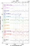 |
Fig. 1. Q branch of the fundamental rovibrational ν2 band of H3+ (P and R branches are shown in Fig. C.1). The JWST/NIRSpec spectra are continuum-subtracted (Sect. 2.3) and scaled. The H3+ transitions are labeled at the top of the panel and indicated by the dotted black vertical lines. Dashed and dot-dashed gray vertical lines indicate transitions of H2 and H I, respectively. The number below the region name is the scaling factor applied. In this figure, the rest frame is defined by the velocity of the H3+ features. We note that the JWST/NIRSpec spectra have a ∼0.1 μm gap centered around 4.05–4.15 μm that partially affects the Q branch of some of these regions. For IRAS 08572, we masked spectral channels with highly uncertain flux values. |
2.1. H spectroscopy and Galactic observations
The energy level diagram of H3+ is shown in Fig. 2. There are two H3+ spin isomers depending on the total nuclear spin I: ortho-H3+ with I = 3/2 and quantum number K = 3n; and para-H3+ with I = 1/2 and K = 3n ± 1 (green and black levels in Fig. 2, respectively). Due to the selection rules, the (3,3) level of the ground state is metastable and cannot decay radiatively to the lowest ortho-H3+ level (1,0) (see e.g., Oka 2013; Miller et al. 2020 for a detailed description of the H3+ spectroscopy). Therefore, H3+ molecules tend to accumulate in the (1,1), (1,0), and (3,3) levels in the conditions of the ISM. More specifically, Galactic observations of H3+ in both diffuse and dense (n(H2)∼104 − 5 cm−3) clouds detect only the (1,1) and (1,0) absorptions (McCall et al. 1999; Indriolo & McCall 2012), whereas the higher excitation (3,3) absorptions are observed only toward the GC. A (2,2) absorption has been uniquely detected along a line of sight (GC IRS 3) toward the circumnuclear disk (CND) of the GC (Goto et al. 2008, 2014; Oka et al. 2019).
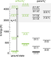 |
Fig. 2. Energy level diagram of H3+. The gray shaded area marks the v2 = 1 levels. Ortho-H3+ levels are in green and para-H3+ in black. The metastable and ground rotational levels are indicated by thicker lines. For the ground state, the quantum numbers of each level are (J, K) and for the v2 = 1 levels, (J,G,K). The detected transitions connect the ground and the v2 = 1 states. The arrows show how the (3,0) level can be populated by IR pumping through the R(1,0) and P(3,0) transitions. |
2.2. H kinematics: Outflows and inflows
The absorptions were fitted using Gaussian profiles. As in Pereira-Santaella et al. (2024), we tied the line-of-sight velocity of all the H3+ transitions to a common value. We also tied the velocity dispersion of the transitions of the same branch, but allowed it to vary between the three branches to account for the variation of the resolving power of NIRSpec (see Appendix A).
In 50% of the sample (five objects), the H3+ absorptions are blueshifted 50–180 km s−1 relative to the molecular and ionized gas traced by the high-J pure rotational H2 and H recombination lines observed by NIRSpec. This indicates that the clouds with H3+ are outflowing (Fig. A.1). These H3+ outflow velocities are lower than those measured using the OH 119 μm and the CO(2–1) 230.5 GHz lines for these targets (∼300–500 km s−1; Veilleux et al. 2013; Lamperti et al. 2022). Thus, it is possible that H3+ traces clouds close to the outflow launching sites before the gas has been fully accelerated (e.g., González-Alfonso et al. 2017; Pereira-Santaella et al. 2020). Only in the southern nucleus of NGC 3256 are the H3+ absorptions redshifted, by ∼70–140 km s−1, suggesting an inflow.
2.3. H column densities and location of the clouds
We estimated the column density of each H3+ level using the standard relation for optically thin lines:
 (1)
(1)
where Wλ is the equivalent width (EW) in wavelength units of the absorptions, Nl the column density of the lower level, λ the wavelength of the transition, c the speed of light, Aul the Einstein A-coefficient of the transition, and gl and gu the statistical weights of the lower and upper levels, respectively.
In order to measure Wλ, we used a spline-interpolated baseline to estimate the continuum level. We note that the EW of the P(2,2) and P(2,1) transitions (affected by the 4.27 μm CO2 ice and gas absorptions) and the R(3,3)l and R(3,3)u transitions (affected by the 3.4–3.6 μm stellar continuum features and PAH aliphatic bands) are relatively uncertain.
We find that, for the same level, the column densities derived from the shorter wavelength branches are lower than those derived from longer wavelength branches. In particular, for the (1,1) and (3,3) levels, which show absorptions in two or three branches, the R branch (3.4–3.7 μm) columns are, on average, ∼1.5 times lower than those derived from the Q branch (3.9–4.0 μm), and the latter are ∼1.3 times lower than those derived from the P branch (4.2–4.4 μm).
In these objects, the stellar continuum dominates the near-IR continuum up to ∼3.5–3.9 μm, while the hot-dust continuum dominates the spectra at longer wavelengths (Donnan et al. 2024). Thus, the column-density discrepancies can be explained if the H3+ absorptions are primarily produced toward the compact hot-dust continuum (r < 20 pc in some of these objects; Rich et al. 2023; García-Bernete et al. 2024b; Inami et al. 2022), whereas the more spatially extended stellar continuum, not affected by the H3+ absorptions, reduces the observed EW at shorter wavelengths. This also implies that the spatial extent of the H3+ clouds is more similar to that of the compact dust continuum than to the extended stellar continuum. The nondetection of the R(3,3)u line at 3.43 μm (where the stellar continuum dominates) in 9 out of 10 regions further corroborates the proposed explanation. R(3,3)u should have an EW that is > 2–10 times higher than the derived upper limits based on the P(3,3) absorption at 4.35 μm.
3. Discussion
3.1. H2 Ionization rate: Cosmic rays and X-rays
For low ζH2/nH (< 10−17 cm3 s−1), where nH = n(H) + 2n(H2), the H3+ abundance is proportional to ζH2/nH. For higher ζH2/nH, the molecular fraction, fH2 = 2n(H2)/nH, decreases, reducing the formation rate of H3+, and the increased abundance of free electrons, xe, enhances the dissociative recombinations of H3+. Hence, in this limit, the H3+ abundance decreases for increasing ζH2/nH in both XDR and CRDR (see Maloney et al. 1996; Le Petit et al. 2016; Neufeld & Wolfire 2017).
Thus, as a first step to estimate ζH2, we calculated the H3+ fractional abundance, N(H3+)/NH. We estimated NH from the extinction affecting the 3.4–4.4 μm continuum where the H3+ absorptions are detected. This is justified because the H3+ absorptions are produced in clouds close to the continuum source (Sect. 3.2), which are likely the same clouds that extinguish this 3.4–4.4 μm continuum. We used the method presented by Donnan et al. (2024) to model the differential extinction of the 3–28 μm continuum observed with NIRSpec and MIRI/MRS for these sources. We obtain an extinction at ∼4 μm equivalent to NH (2–19)×1022 cm−2 (Table B.4). This is approximately equivalent to an optical depth τ4μm of about ∼0.4 − 51. Higher τ4μm would make this 3.4–4.4 μm dust continuum too weak to be detected. However, we note that the NH affecting the longer-wavelength continuum in these (U)LIRGs is considerably larger due to differential extinction effects.
Figure 3 shows that, for the detections, the average H3+ abundance is ∼2 × 10⁻⁷, which is slightly higher than the average abundance in the GC, of namely ∼0.7 × 10⁻⁷ (Oka et al. 2019). Interestingly, the N(H3+) upper limits for the three Sy AGN, that is, the less-obscured AGN in the sample where high-ionization lines are detected, imply low H3+ abundances < 4 × 10⁻⁸. This result is also consistent with the low H3+ EW measured in the Sy 2 AGN NGC 1068 (Geballe et al. 2015). This can be explained if the X-ray radiation from the AGN induces a sufficiently high ζH2 to suppress the formation of H3+ by both decreasing fH2 and increasing xe. The middle panel of Fig. 3 shows the relation between the observed 2–10 keV X-ray luminosity, Lobs(2–10 keV), and the H3+ abundance. The three Sy AGN have the highest Lobs(2–10 keV) and the most stringent upper limits on the H3+ abundance. This suggests that X-rays might be limiting the formation of H3+. We also estimated ζH2 due to X-rays by combining Eqs. 12 and 15 from Maloney et al. (1996). For an NH of 1023 cm−2, ζH2/s−1 = 1.9 × 10⁻¹⁴Fx/(erg s−1 cm−2), where Fx is the incident X-ray flux. Therefore, an observed X-ray luminosity of 1043 erg s−1 –which is similar to that of the brightest Sy AGN in the sample– at 50 pc implies ζH2 ∼6 × 10⁻¹³ s−1, which for the average n(H2) of 102 − 3 cm−3 (Sect. 3.2) can place these objects in the regime where the H3+ abundance decreases with increasing ζH2 (right side of the right panel of Fig. 3).
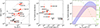 |
Fig. 3. H3+ fractional abundance. Left panel: H3+ vs. H column densities. The H column density corresponds to the obscuring material of the ∼4 μm continuum derived from the continuum differential extinction model (Sect. 3.1). The dashed lines indicate constant H3+ fractional abundances between 10−6 and 10−8 in steps of 1 dex. The red circles are the observed (U)LIRGs. The black star corresponds to the average columns in the GC from Goto et al. (2008) and Oka et al. (2019). Upper limits for Seyfert-type AGN are indicated by the empty black squares. Middle panel: H3+ fractional abundance as a function of the observed 2–10 keV X-ray luminosity. Right panel: Blue shaded area is the predicted H3+ fractional abundance (left y-axis) as a function of ζH2/nH estimated using Eq. 2 from Neufeld & Wolfire (2017) for xe in the range (1.5–5) × 10−4 (Sect. 3.1). The horizontal red shaded area indicates the range of H3+ fractional abundances measured in these (U)LIRGs. The dashed green line (right y-axis) is fH2 as function of ζH2/nH using Eq. 2 from González-Alfonso et al. (2013). |
In this section we use the observed instead of the intrinsic X-ray luminosities because the H3+ absorptions originate at the outer obscuring layers (NH ∼ 1023 cm−2) in objects with a total NH of up to 1025 cm−2, and thus a significant part of the intrinsic X-ray emission has likely been absorbed by more internal gas and dust layers.
The right panel of Fig. 3 shows the predicted H3+ abundance as a function of ζH2/nH derived using Eq. 2 from Neufeld & Wolfire (2017) at T = 300 K. Following González-Alfonso et al. (2013), we assumed xe in the range (1.5–5) × 10−4 and fH2 given by their Eq. 2. This simplified approximation ignores most of the H3+ chemical reactions, but captures the two key elements, xe and fH2, which determine its abundance in diffuse and translucent clouds (Dalgarno 2006; Shaw & Ferland 2021). From the H3+ fractional abundance of the (U)LIRGs, (0.5–5.5) × 10−7, we estimate a ζH2/nH of between 10−18 and > 1.3 × 10⁻¹⁷ cm3 s−1. The average n(H2) is ∼102.5 cm−3 (Sect. 3.2), and so the resulting ζH2 are between ∼3 × 10⁻¹⁶ and > 4 × 10⁻¹⁵ s−1.
The origin of the H3+ detections –either X-rays or cosmic rays– is difficult to constrain. The effects of both X-rays and cosmic rays on the gas are similar (e.g., Glassgold et al. 2012; Wolfire et al. 2022). Here, we consider the fact that cosmic rays can penetrate much larger column densities than X-rays. Therefore, if X-ray radiation from an AGN is present in these (U)LIRGs, it would be absorbed by the internal gas layers, preventing it from reaching the more external gas clouds. This hypothesis is supported by observations showing that (U)LIRGs are under-luminous in hard X-rays (Imanishi & Terashima 2004; Teng et al. 2015; Ricci et al. 2021). Similarly, low-energy-proton cosmic rays (< 10–100 MeV) have stopping ranges of below 1024 cm−2 (Padovani et al. 2018), and so they are likely absorbed by the internal gas layers too. However, cosmic rays of more energetic protons (100–180 MeV), with stopping ranges of 1024 − 25 cm−2, can deposit their energy over large columns comparable to those of (U)LIRGs. Therefore, we consider that ionization by > 100 MeV cosmic rays is more plausible than X-ray ionization in these objects. These cosmic rays are more energetic than those in our Galaxy, which have typical energies of 2–10 MeV (Indriolo et al. 2009). Thus, depending on both the cosmic-ray energy spectrum and the total NH of (U)LIRGs, the intrinsic cosmic-ray luminosity can be > 20 times2 higher than in the GC for the same ζH2.
Other molecular ions like OH+, H2O+, and H3O+, which can form via reactions with H3+, have been detected in (U)LIRGs hosting Seyfert AGN (including NGC 7469, which is part of this sample; van der Werf et al. 2010; Aalto et al. 2011; Pereira-Santaella et al. 2013, 2014). The low H3+ abundance in these AGN supports the idea that these ions form through reaction chains involving H+ and O+, instead of H3+ (Hollenbach et al. 2012; González-Alfonso et al. 2013; Gómez-Carrasco et al. 2014).
3.2. Physical conditions of the H3+ clouds
Previous studies of the H3+ absorptions toward the GC indicate that H3+ traces a warm (T ∼ 200–500 K) diffuse (nH < 100 cm−3) gas phase with a high cosmic-ray ionization rate (ζcr ∼ (1 − 10)×10−14 s−1; Goto et al. 2008; Le Petit et al. 2016; Oka et al. 2019). In this section, we investigate the similarity between the conditions in these (U)LIRGs and those of the GC.
A major difference is that the observed H3+ column densities in these objects, N(H3+) = (7 − 93)×1015 cm−2, are 2–30 times higher than in the GC. The H3+ excitation is also different in some objects. Figure 4 shows column density ratios between various H3+ levels that can be used to characterize the physical conditions of these clouds (e.g., Goto et al. 2008; Le Petit et al. 2016). As shown in the top panel of Fig. 4, contrary to Galactic diffuse and dense clouds, the (3,3) lines are detected in all these (U)LIRGs. Thus, this ratio also suggests that the detections in (U)LIRGs are not produced in extended diffuse gas halos (see also Sect. 2.3).
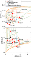 |
Fig. 4. Ratio between the column densities of H3+ levels: (1,0)/(1,1) vs. (3,3)/(1,1) (top); and (3,3)/(2,2) vs. (3,3)/(1,1) (bottom). Symbols as in Fig. 3. The blue diamond corresponds to the excited GC IRS 3 line of sight toward the GC, and the dark blue square in the top panel to diffuse and dense molecular clouds in the Galactic disk. The background grids show the ratios predicted by NLTE models. The green (orange) lines mark the ratios for the temperature, in K, (density, in log cm−3) indicated by the colored labels. |
In Fig. 4, we also plot a grid of nonlocal thermodynamic equilibrium (NLTE) models calculated using RADEX (van der Tak et al. 2007) with the H3+–H2 collisional coefficients from Oka & Epp (2004). The RADEX grid covers H2 densities,  /cm−3, of between 1.0 and 6.0, and kinetic temperatures, Tkin, of between 15 and 600 K in logarithmic steps.
In three targets, VV 114 NE and SW-s1, and IRAS 14348-NE, the (2,2) absorptions are not detected and the ratios are similar to those in the GC. Thus, for these nuclei, the gas temperature is 150–300 K and n(H2) < 100 cm−3, which are comparable to those of the GC (Goto et al. 2008; Le Petit et al. 2016; Oka et al. 2019). We note that some of the observed (1,0)/(1,1) ratios are not well reproduced by these NLTE grids (top panel of Fig. 4). The formation of H3+ is highly exothermic (1.74 eV≡20190 K) and this can affect the observed populations of the (1,0) and (1,1) levels, which do not always reach the ortho-para thermal equilibrium (Le Bourlot et al. 2024). Therefore, formation pumping might explain the low (1,0)/(1,1) ratio in some of these regions. The remaining targets have clear (2,2) detections. For most objects, the (3,3)/(2,2) ratios (bottom panel of Fig. 4) are comparable, within the uncertainties, with that of the singular GC IRS 3 line of sight (Goto et al. 2008, 2014), and indicate warmer (Tkin = 250–500 K) and denser (log n(H2) = 102 − 3 cm−3) clouds.
Some absorptions cannot be explained by these NLTE models. In particular, the absorptions from the (3,0) and (2,1) levels, detected in IRAS 07251, IRAS 08572, and IRAS 14348-SW (Table B.4), are 5–50 times stronger than those predicted by the best-fit NLTE models. However, these absorptions can be explained by IR pumping. When the IR pumping rate, which is proportional to the ambient IR radiation field ϕIR, is higher than the collisional rate, which is proportional to n(H2), the (3,0) level, and similarly the (2,1) level, can be populated by the mechanism shown in Fig. 2 (see also Sect. 5.5 in Goto et al. 2008). Therefore, in these three objects, the ϕIR/n(H2) ratio is likely sufficiently high to make IR pumping the dominant excitation mechanism. We verified this scenario by creating a grid of full radiative transfer models, including the effects of IR pumping, which are able to reproduce these absorptions (Appendix D).
4. Summary and conclusions
We analyzed the fundamental 3.4 − 4.4 μm rovibrational band of H3+ in the spectra of 20 regions (nuclei and bright clumps) selected in 12 local (d ∼ 39–400 Mpc) (U)LIRGs observed by JWST/NIRSpec. The H3+ band is detected in 13 out of 20 regions. It is seen in emission for the first time in the ISM in three of these regions, and in absorption in the remaining ten regions. The main results from our analysis of the H3+ absorptions are as follows:
-
H3+cloud location. The H3+ absorptions are primarily produced toward the hot dust continuum, which dominates the spectra at > 3.5–3.9 μm, rather than toward the stellar continuum. Consequently, the clouds traced by these H3+ absorptions are likely associated with the compact (r < 20 pc in some cases) dust continuum source.
-
Nondetection ofH3+in Seyfert AGN. The H3+ absorptions are undetected in the Seyfert-like (U)LIRGs. These objects are among those least obscured in the sample. Thus, they host mildly obscured AGN whose X-ray radiation might be limiting the abundance of H3+ by decreasing the molecular fraction fH2 and increasing the free electron abundance xe.
-
Low-velocity molecular outflows and inflows. In five regions (50% of the sample), the H3+ absorptions are blueshifted by 50–180 km s−1 relative to the ionized and warm/hot molecular gas. These outflow velocities are lower than those measured using OH 119 μm or rotational CO lines in these objects. This suggests that H3+ traces clouds closer to the outflow launching sites before it has been fully accelerated. In one region, the absorptions are redshifted by 70–140 km s−1 suggesting inflowing gas.
-
H3+column densities, abundances, andH2ionization rate. The H3+ column densities are (0.7–9.3) × 1016 cm−2 , which corresponds to fractional H3+ abundances of (0.5–5.5) × 10−7. Using a simple model for H3+ abundance in translucent clouds, we estimate ζH2/nH to be between 10−18 and > 1.3 × 10⁻¹⁷ cm3 s−1. For n(H2)∼102.5 cm−3 (see below), ζH2 are between 3 × 10⁻¹⁶ and > 4 × 10⁻¹⁵ s−1. Energetic cosmic rays with E > 100–180 MeV have stopping ranges of NH ∼1024 − 25 cm−2, comparable to the total NH of (U)LIRGs, and so they are a plausible origin for these ζH2.
-
NLTE models and excitation ofH3+. We find that in most of the regions that show H3+ absorption (seven out of ten), the H3+ excitation is consistent with warm translucent molecular clouds (Tkin ∼ 250–500 K and n(H2)∼102 − 3 cm−3) excited by inelastic collisions with H2. These conditions are similar to those observed in the extreme line-of-sight GC IRS 3 toward the CND of the GC. In three objects, absorptions from the (3,0) and (2,1) levels of o-H3+ and p-H3+, respectively, are detected for the first time in the ISM. These objects require IR pumping excitation to explain these excited absorptions.
These results show the potential of JWST to detect the key molecule H3+ in extragalactic objects. This will allow constraint of the ionization and chemistry of the molecular ISM (i.e., the initial conditions for star formation) using H3+ for the first time in large samples of galaxies.
For a screen extinction law NH/τ4μm ∼ 3.8 × 1022 cm−2 (Bohlin et al. 1978; Chiar & Tielens 2006).
This factor is the ratio between the effective ζH2 for NH = 1022 cm−2 and 1025 cm−2 given by Eq. F.1 of Padovani et al. (2018) for the cosmic-ray energy spectrum ℋ.
Acknowledgments
We are grateful to Octavio Roncero for insightful discussions about H3+ and reading the manuscript. We thank the referee, David Neufeld, for a careful reading of the manuscript and a constructive report. The authors acknowledge the GOALS and the NIRSpec GTO teams for developing their observing programs. MPS acknowledges support under grants RYC2021-033094-I and CNS2023-145506 funded by MCIN/AEI/10.13039/501100011033 and the European Union NextGenerationEU/PRTR. MPS, EGA, MGSM, and JRG acknowledge funding support under grant PID2023-146667NB-I00 funded by the Spanish MCIN/AEI/10.13039/501100011033. EGA acknowledges grants PID2019-105552RB-C4 and PID2022-137779OB-C41 funded by the Spanish MCIN/AEI/10.13039/501100011033. IGB is supported by the Programa Atracción de Talento Investigador “César Nombela” via grant 2023-T1/TEC-29030 funded by the Community of Madrid. FD acknowledges support from STFC through studentship ST/W507726/1. MGSM acknowledges support from the NSF under grant CAREER 2142300. MP acknowledges grant PID2021-127718NB-I00 funded by the Spanish Ministry of Science and Innovation/State Agency of Research (MICIN/AEI/ 10.13039/501100011033). DR acknowledges support from STFC through grants ST/S000488/1 and ST/W000903/1. This work is based on observations made with the NASA/ESA/CSA James Webb Space Telescope. The data were obtained from the Mikulski Archive for Space Telescopes at the Space Telescope Science Institute, which is operated by the Association of Universities for Research in Astronomy, Inc., under NASA contract NAS 5-03127 for JWST; and from the European JWST archive (eJWST) operated by the ESAC Science Data Centre (ESDC) of the European Space Agency. These observations are associated with programs #1267, #1328 and #3368.
References
- Aalto, S., Costagliola, F., van der Tak, F., & Meijerink, R. 2011, A&A, 527, A69 [NASA ADS] [CrossRef] [EDP Sciences] [Google Scholar]
- Argyriou, I., Glasse, A., Law, D. R., et al. 2023, A&A, 675, A111 [NASA ADS] [CrossRef] [EDP Sciences] [Google Scholar]
- Armus, L., Mazzarella, J. M., Evans, A. S., et al. 2009, PASP, 121, 559 [Google Scholar]
- Armus, L., Lai, T., Vivian, U., et al. 2023, ApJ, 942, L37 [NASA ADS] [CrossRef] [Google Scholar]
- Barcos-Muñoz, L., Leroy, A. K., Evans, A. S., et al. 2017, ApJ, 843, 117 [CrossRef] [Google Scholar]
- Bianchin, M., Vivian, U., Song, Y., et al. 2024, ApJ, 965, 103 [NASA ADS] [CrossRef] [Google Scholar]
- Blustin, A. J., Branduardi-Raymont, G., Behar, E., et al. 2003, A&A, 403, 481 [NASA ADS] [CrossRef] [EDP Sciences] [Google Scholar]
- Bohlin, R. C., Savage, B. D., & Drake, J. F. 1978, ApJ, 224, 132 [Google Scholar]
- Böker, T., Arribas, S., Lützgendorf, N., et al. 2022, A&A, 661, A82 [NASA ADS] [CrossRef] [EDP Sciences] [Google Scholar]
- Buiten, V. A., van der Werf, P. P., Viti, S., et al. 2024, ApJ, 966, 166 [NASA ADS] [CrossRef] [Google Scholar]
- Bushouse, H., Eisenhamer, J., Dencheva, N., et al. 2023, JWST Calibration Pipeline https://doi.org/10.5281/zenodo.7829329 [Google Scholar]
- Chiar, J. E., & Tielens, A. G. G. M. 2006, ApJ, 637, 774 [NASA ADS] [CrossRef] [Google Scholar]
- Clements, D. L., McDowell, J. C., Shaked, S., et al. 2002, ApJ, 581, 974 [NASA ADS] [CrossRef] [Google Scholar]
- Costagliola, F., Sakamoto, K., Muller, S., et al. 2015, A&A, 582, A91 [NASA ADS] [CrossRef] [EDP Sciences] [Google Scholar]
- Dalgarno, A. 2006, Proc. Nat. Acad. Sci., 103, 12269 [NASA ADS] [CrossRef] [Google Scholar]
- Donnan, F. R., García-Bernete, I., Rigopoulou, D., et al. 2023, MNRAS, 519, 3691 [CrossRef] [Google Scholar]
- Donnan, F. R., García-Bernete, I., Rigopoulou, D., et al. 2024, MNRAS, 529, 1386 [NASA ADS] [CrossRef] [Google Scholar]
- Drossart, P., Maillard, J. P., Caldwell, J., et al. 1989, Nature, 340, 539 [NASA ADS] [CrossRef] [Google Scholar]
- Duc, P. A., Mirabel, I. F., & Maza, J. 1997, A&AS, 124, 533 [NASA ADS] [CrossRef] [EDP Sciences] [Google Scholar]
- Falstad, N., Aalto, S., König, S., et al. 2021, A&A, 649, A105 [NASA ADS] [CrossRef] [EDP Sciences] [Google Scholar]
- García-Bernete, I., Rigopoulou, D., Aalto, S., et al. 2022a, A&A, 663, A46 [NASA ADS] [CrossRef] [EDP Sciences] [Google Scholar]
- García-Bernete, I., Rigopoulou, D., Alonso-Herrero, A., et al. 2022b, A&A, 666, L5 [NASA ADS] [CrossRef] [EDP Sciences] [Google Scholar]
- García-Bernete, I., Rigopoulou, D., Alonso-Herrero, A., et al. 2022c, MNRAS, 509, 4256 [Google Scholar]
- García-Bernete, I., Alonso-Herrero, A., Rigopoulou, D., et al. 2024a, A&A, 681, L7 [NASA ADS] [CrossRef] [EDP Sciences] [Google Scholar]
- García-Bernete, I., Pereira-Santaella, M., González-Alfonso, E., et al. 2024b, A&A, 682, L5 [NASA ADS] [CrossRef] [EDP Sciences] [Google Scholar]
- Geballe, T. R., & Oka, T. 1996, Nature, 384, 334 [NASA ADS] [CrossRef] [Google Scholar]
- Geballe, T. R., Goto, M., Usuda, T., Oka, T., & McCall, B. J. 2006, ApJ, 644, 907 [NASA ADS] [CrossRef] [Google Scholar]
- Geballe, T. R., Mason, R. E., & Oka, T. 2015, ApJ, 812, 56 [NASA ADS] [CrossRef] [Google Scholar]
- Gibb, E. L., Brittain, S. D., Rettig, T. W., et al. 2010, ApJ, 715, 757 [NASA ADS] [CrossRef] [Google Scholar]
- Glassgold, A. E., Galli, D., & Padovani, M. 2012, ApJ, 756, 157 [Google Scholar]
- Gómez-Carrasco, S., Godard, B., Lique, F., et al. 2014, ApJ, 794, 33 [CrossRef] [Google Scholar]
- González-Alfonso, E., Cernicharo, J., van Dishoeck, E. F., Wright, C. M., & Heras, A. 1998, ApJ, 502, L169 [CrossRef] [Google Scholar]
- González-Alfonso, E., Fischer, J., Graciá-Carpio, J., et al. 2012, A&A, 541, A4 [NASA ADS] [CrossRef] [EDP Sciences] [Google Scholar]
- González-Alfonso, E., Fischer, J., Bruderer, S., et al. 2013, A&A, 550, A25 [NASA ADS] [CrossRef] [EDP Sciences] [Google Scholar]
- González-Alfonso, E., Fischer, J., Sturm, E., et al. 2015, ApJ, 800, 69 [CrossRef] [Google Scholar]
- González-Alfonso, E., Fischer, J., Spoon, H. W. W., et al. 2017, ApJ, 836, 11 [Google Scholar]
- González-Alfonso, E., García-Bernete, I., Pereira-Santaella, M., et al. 2024, A&A, 682, A182 [NASA ADS] [CrossRef] [EDP Sciences] [Google Scholar]
- Gorski, M. D., Aalto, S., König, S., et al. 2023, A&A, 670, A70 [NASA ADS] [CrossRef] [EDP Sciences] [Google Scholar]
- Goto, M., Usuda, T., Nagata, T., et al. 2008, ApJ, 688, 306 [NASA ADS] [CrossRef] [Google Scholar]
- Goto, M., Geballe, T. R., Indriolo, N., et al. 2014, ApJ, 786, 96 [CrossRef] [Google Scholar]
- Grimes, J. P., Heckman, T., Hoopes, C., et al. 2006, ApJ, 648, 310 [NASA ADS] [CrossRef] [Google Scholar]
- Hollenbach, D., Kaufman, M. J., Neufeld, D., Wolfire, M., & Goicoechea, J. R. 2012, ApJ, 754, 105 [Google Scholar]
- Hung, C.-L., Sanders, D. B., Casey, C. M., et al. 2014, ApJ, 791, 63 [NASA ADS] [CrossRef] [Google Scholar]
- Imanishi, M., & Terashima, Y. 2004, AJ, 127, 758 [NASA ADS] [CrossRef] [Google Scholar]
- Inami, H., Surace, J., Armus, L., et al. 2022, ApJ, 940, L6 [NASA ADS] [CrossRef] [Google Scholar]
- Indriolo, N., & McCall, B. J. 2012, ApJ, 745, 91 [NASA ADS] [CrossRef] [Google Scholar]
- Indriolo, N., Fields, B. D., & McCall, B. J. 2009, ApJ, 694, 257 [NASA ADS] [CrossRef] [Google Scholar]
- Iwasawa, K., Sanders, D. B., Teng, S. H., et al. 2011, A&A, 529, A106+ [NASA ADS] [CrossRef] [EDP Sciences] [Google Scholar]
- Jakobsen, P., Ferruit, P., Alves de Oliveira, C., et al. 2022, A&A, 661, A80 [NASA ADS] [CrossRef] [EDP Sciences] [Google Scholar]
- Labiano, A., Argyriou, I., Álvarez-Márquez, J., et al. 2021, A&A, 656, A57 [NASA ADS] [CrossRef] [EDP Sciences] [Google Scholar]
- Lamperti, I., Pereira-Santaella, M., Perna, M., et al. 2022, A&A, 668, A45 [NASA ADS] [CrossRef] [EDP Sciences] [Google Scholar]
- Le Bourlot, J., Roueff, E., Le Petit, F., et al. 2024, Mol. Phys., 122, e2182612 [Google Scholar]
- Le Petit, F., Ruaud, M., Bron, E., et al. 2016, A&A, 585, A105 [NASA ADS] [CrossRef] [EDP Sciences] [Google Scholar]
- Lípari, S., Díaz, R., Taniguchi, Y., et al. 2000, AJ, 120, 645 [CrossRef] [Google Scholar]
- Lira, P., Ward, M., Zezas, A., Alonso-Herrero, A., & Ueno, S. 2002, MNRAS, 330, 259 [CrossRef] [Google Scholar]
- Lutz, D., Sturm, E., Janssen, A., et al. 2020, A&A, 633, A134 [NASA ADS] [CrossRef] [EDP Sciences] [Google Scholar]
- Maloney, P. R., Hollenbach, D. J., & Tielens, A. G. G. M. 1996, ApJ, 466, 561 [Google Scholar]
- McCall, B. J., Geballe, T. R., Hinkle, K. H., & Oka, T. 1999, ApJ, 522, 338 [NASA ADS] [CrossRef] [Google Scholar]
- McCall, B. J., Hinkle, K. H., Geballe, T. R., et al. 2002, ApJ, 567, 391 [NASA ADS] [CrossRef] [Google Scholar]
- Miller, S., Tennyson, J., Geballe, T. R., & Stallard, T. 2020, Rev. Mod. Phys., 92 [CrossRef] [Google Scholar]
- Mizus, I. I., Alijah, A., Zobov, N. F., et al. 2017, MNRAS, 468, 1717 [NASA ADS] [CrossRef] [Google Scholar]
- Nardini, E., Risaliti, G., Watabe, Y., Salvati, M., & Sani, E. 2010, MNRAS, 405, 2505 [NASA ADS] [Google Scholar]
- Neufeld, D. A., & Wolfire, M. G. 2017, ApJ, 845, 163 [Google Scholar]
- Ohyama, Y., Terashima, Y., & Sakamoto, K. 2015, ApJ, 805, 162 [Google Scholar]
- Oka, T. 2013, Chem. Rev., 113, 8738 [NASA ADS] [CrossRef] [Google Scholar]
- Oka, T., & Epp, E. 2004, ApJ, 613, 349 [NASA ADS] [CrossRef] [Google Scholar]
- Oka, T., Geballe, T. R., Goto, M., et al. 2019, ApJ, 883, 54 [Google Scholar]
- Osterbrock, D. E., & Martel, A. 1993, ApJ, 414, 552 [Google Scholar]
- Padovani, M., Ivlev, A. V., Galli, D., & Caselli, P. 2018, A&A, 614, A111 [NASA ADS] [CrossRef] [EDP Sciences] [Google Scholar]
- Padovani, M., Ivlev, A. V., Galli, D., et al. 2020, Space. Sci. Rev., 216, 29 [NASA ADS] [CrossRef] [Google Scholar]
- Papadopoulos, P. P. 2010, ApJ, 720, 226 [NASA ADS] [CrossRef] [Google Scholar]
- Pereira-Santaella, M., Alonso-Herrero, A., Santos-Lleo, M., et al. 2011, A&A, 535, A93 [NASA ADS] [CrossRef] [EDP Sciences] [Google Scholar]
- Pereira-Santaella, M., Spinoglio, L., Busquet, G., et al. 2013, ApJ, 768, 55 [Google Scholar]
- Pereira-Santaella, M., Spinoglio, L., van der Werf, P. P., & Piqueras López, J. 2014, A&A, 566, A49 [NASA ADS] [CrossRef] [EDP Sciences] [Google Scholar]
- Pereira-Santaella, M., Colina, L., García-Burillo, S., et al. 2020, A&A, 643, A89 [NASA ADS] [CrossRef] [EDP Sciences] [Google Scholar]
- Pereira-Santaella, M., Colina, L., García-Burillo, S., et al. 2021, A&A, 651, A42 [NASA ADS] [CrossRef] [EDP Sciences] [Google Scholar]
- Pereira-Santaella, M., Álvarez-Márquez, J., García-Bernete, I., et al. 2022, A&A, 665, L11 [NASA ADS] [CrossRef] [EDP Sciences] [Google Scholar]
- Pereira-Santaella, M., González-Alfonso, E., García-Bernete, I., García-Burillo, S., & Rigopoulou, D. 2024, A&A, 681, A117 [NASA ADS] [CrossRef] [EDP Sciences] [Google Scholar]
- Perna, M., Arribas, S., Catalán-Torrecilla, C., et al. 2020, A&A, 643, A139 [NASA ADS] [CrossRef] [EDP Sciences] [Google Scholar]
- Perna, M., Arribas, S., Pereira Santaella, M., et al. 2021, A&A, 646, A101 [EDP Sciences] [Google Scholar]
- Ricci, C., Privon, G. C., Pfeifle, R. W., et al. 2021, MNRAS, 506, 5935 [NASA ADS] [CrossRef] [Google Scholar]
- Rich, J., Aalto, S., Evans, A. S., et al. 2023, ApJ, 944, L50 [CrossRef] [Google Scholar]
- Rodriguez-Gomez, V., Genel, S., Vogelsberger, M., et al. 2015, MNRAS, 449, 49 [Google Scholar]
- Shaw, G., & Ferland, G. J. 2021, ApJ, 908, 138 [NASA ADS] [CrossRef] [Google Scholar]
- Teng, S. H., Rigby, J. R., Stern, D., et al. 2015, ApJ, 814, 56 [Google Scholar]
- Trafton, L. M., Geballe, T. R., Miller, S., Tennyson, J., & Ballester, G. E. 1993, ApJ, 405, 761 [NASA ADS] [CrossRef] [Google Scholar]
- van der Tak, F. F. S., Black, J. H., Schöier, F. L., Jansen, D. J., & van Dishoeck, E. F. 2007, A&A, 468, 627 [NASA ADS] [CrossRef] [EDP Sciences] [Google Scholar]
- van der Werf, P. P., Isaak, K. G., Meijerink, R., et al. 2010, A&A, 518, L42 [NASA ADS] [CrossRef] [EDP Sciences] [Google Scholar]
- Veilleux, S., Rupke, D. S. N., Kim, D.-C., et al. 2009, ApJS, 182, 628 [Google Scholar]
- Veilleux, S., Meléndez, M., Sturm, E., et al. 2013, ApJ, 776, 27 [Google Scholar]
- Vivian, U., Lai, T., Bianchin, M., et al. 2022, ApJ, 940, L5 [NASA ADS] [CrossRef] [Google Scholar]
- Wolfire, M. G., Vallini, L., & Chevance, M. 2022, ARA&A, 60, 247 [NASA ADS] [CrossRef] [Google Scholar]
- Wright, G. S., Rieke, G. H., Glasse, A., et al. 2023, PASP, 135, 048003 [NASA ADS] [CrossRef] [Google Scholar]
Appendix A: Sample and data reduction
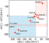 |
Fig. A.1. Comparison between the velocity measured for the H3+ absorptions and that of H2 (x axis) and H recombination lines (y axis). For two objects, no H2 lines are available, so the horizontal line marks the H3+ velocity relative to that of the H recombination lines. The shaded blue and red areas indicate blue and red velocity shifts, respectively. |
Sample of local (U)LIRGs.
We selected all the (U)LIRGs with publicly available high spectral resolution NIRSpec and Mid-Infrared Instrument (MIRI) spectroscopic observations in the JWST archive by July 2024. We excluded few objects, mainly interacting systems whose nuclei are not clearly separated at the angular resolution of JWST/MIRI at ∼20 μm, which is needed for the continuum modeling of each nuclei. The final sample consists of 12 systems (see Table A.1) with data from the Director’s Discretionary Early Release Science (DD-ERS) Program #1328 (PI: L. Armus and A. Evans), the Large Program #3368 (PI: L. Armus and A. Evans), and the Guaranteed Time Observations Program #1267 (PI: D. Dicken; Program lead: T. Böker).
These objects were observed with the high spectral resolution NIRSpec grating G395H using the integral field unit (IFU) mode (Böker et al. 2022). The G395H grating has a resolving power, R, between 1900 and 3600, and covers the spectral range between 2.87 and 5.27 μm (JWST User Documentation). Between ∼3.5 μm and ∼4.3 μm, the spectral range where the H3+ band is observed, R varies between 2400 and 3000. JWST/MIRI observations of these objects were also available for all the bands of the Medium Resolution Spectrograph (MRS; Wright et al. 2023; Argyriou et al. 2023) between 4.9 and 28.1 μm with R = 2300–3700 (Labiano et al. 2021).
For the data reduction, we used the JWST calibration pipeline (version 1.12.4; Bushouse et al. 2023) and the context 1253. We followed the standard reduction recipe complemented by a number of custom steps to mitigate the effect of bad pixels and cosmic rays on the extracted spectra. Further details on the data reduction of the NIRSpec and MIRI/MRS data observations can be found in Pereira-Santaella et al. (2022, 2024) and García-Bernete et al. (2022b, 2024a).
We extracted the spectra of 20 regions within these systems. Sixteen regions correspond to their nuclei, three regions are bright near-IR clumps with strong bursts of star-formation (Inami et al. 2022; García-Bernete et al. 2024b; Buiten et al. 2024), and one region samples the spatially resolved molecular outflow of NGC 3256-S (Pereira-Santaella et al. 2024; Table A.1). We applied an aperture correction to the spectra similar to García-Bernete et al. (2022c).
Appendix B: Properties of the H3+ absorptions
The EW of the detected H3+ absorptions and upper limits are listed in Tables B.1, B.2, and B.3, for the R, Q, and P branches, respectively. Table B.4 shows the total H3+ column densities.
EW of the H3+ R-branch transitions and derived column densities.
EW of the H3+ Q-branch transitions and derived column densities.
EW of the H3+ P-branch transitions and derived column densities.
Column densities of H3+ and H.
Appendix C: Spectra of the H3+ band
Figure C.1 presents the R and P branches of the detected H3+ band. The Q branch is shown in Fig. 1. Figure C.2 shows the spectra of the regions where no H3+ is detected.
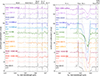 |
Fig. C.1. Similar to Fig. 1, but for the R and P branches of H3+. In the P-branch panel, the He I line at 4.296 μm is indicated by a dashed gray line. |
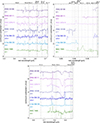 |
Fig. C.2. Similar to Figs. 1 and C.1, but for the non-detections of the H3+ band. The rest frame is defined by the average velocity of the H2 and H transitions. |
Appendix D: Models of the H3+ absorptions including IR pumping
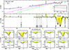 |
Fig. D.1. H3+ absorption in IRAS 07251−0248 and comparison with models. a) Observed 3.4 − 4.4 μm spectrum in IRAS 07251−0248 and adopted spline-interpolated baseline (in blue). The magenta and green lines show the modeled spectra, with the temperatures of the central source Tc and the hot-dust optical depth (τ in the inset) also indicated with colors. b) The continuum-subtracted spectrum (yellow histogram) is compared with the predictions by the two models. The spectra and models for individual lines are plotted in units of velocity in panel c. The vertical dashed line indicates the rest-frame zero velocity determined from the H2 and H I lines. The position of the H2 1 − 1 S(13) 4.068 μm line, which is blended with the P(1,1) 4.070 μm line, is indicated by an arrow. |
We have modeled the H3+ absorption in IRAS 07251−0248 and IRAS 14348−1447 SW using the code described in González-Alfonso et al. (1998). The models assume spherical symmetry with the statistical equilibrium of the H3+ level populations calculated within a shell of gas surrounding a mid-IR source of continuum radiation. The spectra are computed towards the IR source excluding reemission from the flanks. The effects of both radiative pumping by the IR source and collisional excitation are included. The varying parameters are the equivalent radius and temperature of the central source (Rc and Tc), the extinction by the dust mixed with the H3+ (assuming an extinction law with τλ ∝ λ−1.7), the H3+ column density of the shell (N(H3+)), the distance between the H3+ shell and central source (d), the gas conditions (nH2 and Tkin), and the gas velocity field. We assume that the dust mixed with the gas is cold enough such that its reemission does not contribute to the < 4.3 μm continuum.
Figures D.1 and D.2 show the 3.4 − 4.4 μm spectra of IRAS 07251−0248 and IRAS 14348−1447 SW, with the blue lines indicating the adopted spline-interpolated baselines. As discussed in Sect. 2.3, H3+ line absorption is progressively diluted in the stellar continuum at shorter wavelengths, and hence we attempt different spectral shapes for the hot-dust emission characterized by Tc and τ4μm; Rc is then determined by assuming negligible stellar continuum at 4.35 μm (see Donnan et al. 2024). We show in Figs. D.1 and D.2 two models, A (in magenta) and B (in green), with Tc, τλ and the hot-dust emission indicated in panel a. In these figures, the continuum-subtracted spectra in both sources is compared with the predictions by the two models, and details of the observed and modeled line shapes are shown in panels c. The physical parameters of the models are listed in Table D.1.
These models show that, including IR pumping, it is possible to reproduce the absorptions from the (3,0) and (2,1) levels, which are difficult to explain just by collisional excitation with H2 (Sect. 3.2).
All Tables
All Figures
|
Fig. 1. Q branch of the fundamental rovibrational ν2 band of H3+ (P and R branches are shown in Fig. C.1). The JWST/NIRSpec spectra are continuum-subtracted (Sect. 2.3) and scaled. The H3+ transitions are labeled at the top of the panel and indicated by the dotted black vertical lines. Dashed and dot-dashed gray vertical lines indicate transitions of H2 and H I, respectively. The number below the region name is the scaling factor applied. In this figure, the rest frame is defined by the velocity of the H3+ features. We note that the JWST/NIRSpec spectra have a ∼0.1 μm gap centered around 4.05–4.15 μm that partially affects the Q branch of some of these regions. For IRAS 08572, we masked spectral channels with highly uncertain flux values. |
| In the text | |
|
Fig. 2. Energy level diagram of H3+. The gray shaded area marks the v2 = 1 levels. Ortho-H3+ levels are in green and para-H3+ in black. The metastable and ground rotational levels are indicated by thicker lines. For the ground state, the quantum numbers of each level are (J, K) and for the v2 = 1 levels, (J,G,K). The detected transitions connect the ground and the v2 = 1 states. The arrows show how the (3,0) level can be populated by IR pumping through the R(1,0) and P(3,0) transitions. |
| In the text | |
|
Fig. 3. H3+ fractional abundance. Left panel: H3+ vs. H column densities. The H column density corresponds to the obscuring material of the ∼4 μm continuum derived from the continuum differential extinction model (Sect. 3.1). The dashed lines indicate constant H3+ fractional abundances between 10−6 and 10−8 in steps of 1 dex. The red circles are the observed (U)LIRGs. The black star corresponds to the average columns in the GC from Goto et al. (2008) and Oka et al. (2019). Upper limits for Seyfert-type AGN are indicated by the empty black squares. Middle panel: H3+ fractional abundance as a function of the observed 2–10 keV X-ray luminosity. Right panel: Blue shaded area is the predicted H3+ fractional abundance (left y-axis) as a function of ζH2/nH estimated using Eq. 2 from Neufeld & Wolfire (2017) for xe in the range (1.5–5) × 10−4 (Sect. 3.1). The horizontal red shaded area indicates the range of H3+ fractional abundances measured in these (U)LIRGs. The dashed green line (right y-axis) is fH2 as function of ζH2/nH using Eq. 2 from González-Alfonso et al. (2013). |
| In the text | |
|
Fig. 4. Ratio between the column densities of H3+ levels: (1,0)/(1,1) vs. (3,3)/(1,1) (top); and (3,3)/(2,2) vs. (3,3)/(1,1) (bottom). Symbols as in Fig. 3. The blue diamond corresponds to the excited GC IRS 3 line of sight toward the GC, and the dark blue square in the top panel to diffuse and dense molecular clouds in the Galactic disk. The background grids show the ratios predicted by NLTE models. The green (orange) lines mark the ratios for the temperature, in K, (density, in log cm−3) indicated by the colored labels. |
| In the text | |
|
Fig. A.1. Comparison between the velocity measured for the H3+ absorptions and that of H2 (x axis) and H recombination lines (y axis). For two objects, no H2 lines are available, so the horizontal line marks the H3+ velocity relative to that of the H recombination lines. The shaded blue and red areas indicate blue and red velocity shifts, respectively. |
| In the text | |
|
Fig. C.1. Similar to Fig. 1, but for the R and P branches of H3+. In the P-branch panel, the He I line at 4.296 μm is indicated by a dashed gray line. |
| In the text | |
|
Fig. C.2. Similar to Figs. 1 and C.1, but for the non-detections of the H3+ band. The rest frame is defined by the average velocity of the H2 and H transitions. |
| In the text | |
|
Fig. D.1. H3+ absorption in IRAS 07251−0248 and comparison with models. a) Observed 3.4 − 4.4 μm spectrum in IRAS 07251−0248 and adopted spline-interpolated baseline (in blue). The magenta and green lines show the modeled spectra, with the temperatures of the central source Tc and the hot-dust optical depth (τ in the inset) also indicated with colors. b) The continuum-subtracted spectrum (yellow histogram) is compared with the predictions by the two models. The spectra and models for individual lines are plotted in units of velocity in panel c. The vertical dashed line indicates the rest-frame zero velocity determined from the H2 and H I lines. The position of the H2 1 − 1 S(13) 4.068 μm line, which is blended with the P(1,1) 4.070 μm line, is indicated by an arrow. |
| In the text | |
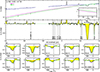 |
Fig. D.2. Same as Fig. D.1 but for IRAS 14348−1447 SW. |
| In the text | |
Current usage metrics show cumulative count of Article Views (full-text article views including HTML views, PDF and ePub downloads, according to the available data) and Abstracts Views on Vision4Press platform.
Data correspond to usage on the plateform after 2015. The current usage metrics is available 48-96 hours after online publication and is updated daily on week days.
Initial download of the metrics may take a while.