| Issue |
A&A
Volume 681, January 2024
|
|
|---|---|---|
| Article Number | A117 | |
| Number of page(s) | 18 | |
| Section | Extragalactic astronomy | |
| DOI | https://doi.org/10.1051/0004-6361/202347942 | |
| Published online | 26 January 2024 | |
The CO-to-H2 conversion factor of molecular outflows
Rovibrational CO emission in NGC 3256-S resolved by JWST/NIRSpec
1
Instituto de Física Fundamental, CSIC,
Calle Serrano 123,
28006
Madrid, Spain
e-mail: This email address is being protected from spambots. You need JavaScript enabled to view it.
2
Universidad de Alcalá, Departamento de Física y Matemáticas, Campus Universitario,
28871 Alcalá de Henares,
Madrid, Spain
3
Department of Physics, University of Oxford,
Keble Road,
Oxford
OX1 3RH, UK
4
Observatorio Astronómico Nacional (OAN-IGN)-Observatorio de Madrid,
Alfonso XII, 3,
28014
Madrid, Spain
Received:
11
September
2023
Accepted:
27
October
2023
Abstract
We analyze JWST/NIRSpec observations of the CO rovibrational υ = 1−0 band at ~4.67 µm around the dust-embedded southern active galactic nucleus (AGN) of NGC 3256 (d = 40 Mpc; LIR = 1011.6 L⊙). We classify the CO υ = 1−0 spectra into three categories based on the behavior of P- and R-branches of the band: (a) both branches in absorption toward the nucleus; (b) P-R asymmetry (P-branch in emission and R-branch in absorption) along the disk of the galaxy; and (c) both branches in emission in the outflow region above and below the disk. In this paper, we focus on the outflow. The CO υ = 1−0 emission can be explained by the vibrational excitation of CO in the molecular outflow by the bright mid-IR ~4.7 µm continuum from the AGN up to r ~ 250 pc. We model the ratios between the P(J+2) and R(J) transitions of the band to derive the physical properties (column density, kinetic temperature, and CO-to-H2 conversion factor, αCO) of the outflowing gas. We find that the 12CO υ = 1−0 emission is optically thick for J < 4, while the 13CO υ = 1−0 emission remains optically thin. From the P(2)/R(0) ratio, we identify a temperature gradient in the outflow from >40 K in the central 100 pc to <15 K at 250 pc, sampling the cooling of the molecular gas in the outflow. We used three methods to derive αCO in eight 100 pc (0″.5) apertures in the outflow by fitting the P( J+2)/R( J) ratios with nonlocal thermodynamic equilibrium (NLTE) models. We obtain low median αCO factors (0.40 - 0.61) × 3.2×10-4/[CO/H2] M⊙ (K km s-1 pc2)-1 in the outflow regions. This implies that outflow rates and energetics might be overestimated if a 1.3−2 times larger ultraluminous infrared galaxy (ULIRG) like αCO is assumed. The reduced αCO can be explained if the outflowing molecular clouds are not virialized. We also report the first extragalactic detection of a broad (σ = 0.0091 µm) spectral feature at 4.645 µm associated with aliphatic deuterium on polycyclic aromatic hydrocarbons (Dn-PAHs).
Key words: galaxies: active / galaxies: evolution / gamma rays: ISM
© The Authors 2024
 Open Access article, published by EDP Sciences, under the terms of the Creative Commons Attribution License (https://creativecommons.org/licenses/by/4.0), which permits unrestricted use, distribution, and reproduction in any medium, provided the original work is properly cited.
This article is published in open access under the Subscribe to Open model. This email address is being protected from spambots. You need JavaScript enabled to view it. to support open access publication.
1 Introduction
Feedback from active galactic nuclei (AGN) has been invoked to explain key properties of galaxies, such as the observed stellar mass function or the quenching of star formation (SF) in quiescent galaxies (e.g., Somerville & Davé 2015). This SF quenching can be caused by the removal of cold gas from the host galaxy by massive outflows. These outflows seem to be dominated by the cold molecular phase and have mass-outflow rates,  , from a few M⊙ yr−1 to >100 M⊙ yr−1 and mass loading factors,
  / star formation rate (SFR), that can exceed 1 in extreme cases; for example, in ultraluminous infrared galaxies (ULIRGs; Harrison et al. 2018; Veilleux et al. 2020).
Rotational CO transitions in the millimeter (mm) and submm ranges are commonly used tracers of cold molecular outflows (e.g., Combes et al. 2013; Cidone et al. 2014; García-Burillo et al. 2015; Pereira-Santaella et al. 2018; Lutz et al. 2020; García-Bernete et al. 2021; Lamperti et al. 2022; Ramos Almeida et al. 2022; Alonso-Herrero et al. 2018, 2019, 2023). To transform the observed CO luminosities (LCO) into molecular masses (Mmol), and the latter into outflow rates, it is necessary to apply a CO-to-H2 conversion factor, αCO = Mmol/LCO. In most cases, this latter is not constrained by the observations and a fixed value is assumed. A range of ~ 1 dex in αCO between 0.3 and 2.0 M⊙ (K km s−1 pc2)−1 has been suggested for outflows from observations of multiple [C I] and rotational CO transitions in a handful of objects (e.g., Dasyra et al. 2016; Cidone et al. 2018; Saito et al. 2022; Ueda et al. 2022). According to these works, possible explanations for the reduced αCO in outflows are: nonvirialized molecular clouds; optically thin rotational CO emission; and/or CO being destroyed, leaving C I. Here, we present an alternative method to estimate the αCO factor using the fundamental rovibrational CO ν = 1−0 4.67 µm band, which can now be observed by the Near Infrared Spectrograph (NIRSpec) instrument (Jakobsen et al. 2022; Böker et al. 2022) on board the James Webb Space Telescope (JWST).
The 4.67 µm rovibrational CO band has previously been observed in extragalactic objects from space with Spitzer and AKARI at low spectral resolution (R < 150), which was insufficient to spectrally resolve the individual transitions of the band (Spoon et al. 2004; Baba et al. 2018, 2022). This band has also been observed from the ground at high spectral resolution R ~ 5000–10000 (to allow for the correction of the atmospheric absorption) in a few deeply obscured objects (e.g., IRAS 08572+3915, NGC 4945, and NGC 4418; Spoon et al. 2003; Geballe et al. 2006; Shirahata et al. 2013; Onishi et al. 2021; Ohyama et al. 2023). All these works focused on detecting the CO rovibrational band in absorption toward dusty bright IR nuclei in order to probe the conditions of the gas close to the central source (AGN and/or compact starburst). In this work, thanks to the sensitivity and spatial resolution of JWST, for the first time we are able to disentangle the rovibrational CO absorption toward the obscured AGN located in the southern nucleus of the luminous infrared (IR) merger NGC 3256 and the spatially extended CO emission around this nucleus using the integral field unit (IFU) of NIRSpec. So far, detections of the CO band in emission have been scarce and only in Galactic sources (e.g., González-Alfonso et al. 2002; Najita et al. 2003; Rettig et al. 2005; Herczeg et al. 2011). With JWST, detection of the CO band in emission is likely to become common in spatially resolved objects hosting bright mid-IR sources.
NGC 3256 is a nearby (d = 40 Mpc; ɀ = 0.00916; 190 pc arcsec−1) gas-rich advanced merger (projected nuclear separation of < 1 kpc) with a high IR luminosity (LIR = 1011.6 L⊙), which places it in the luminous IR galaxy (LIRG) range. The southern component of NGC 3256 (NGC 3256 S) is an edge-on disk with a position angle (PA) of ~90º. It is located in front of the northern component, which is an almost face-on disk (see e.g., Sakamoto et al. 2014).
The northern component is powered by a bright starburst with a nuclear SFR of ~15 M⊙ yr−1 (Lira et al. 2008). The southern component instead hosts an extremely dust-embedded nucleus with a very deep 9.7 µm silicate absorption feature (Pereira-Santaella et al. 2010; Díaz-Santos et al. 2010). The modeling of near-IR, mid-IR, and X-ray observations of the southern nucleus suggests that it is powered by a low-luminosity (L2-10 keV ~ 1040erg s−1) obscured AGN (Ohyama et al. 2015). However, because of the extreme dust obscuration, no high-ionization |transitions or direct X-ray emission are detected from the AGN (e.g., Lira et al. 2002; Alonso-Herrero et al. 2012; Pereira-Santaella et al. 2011).
This AGN has a collimated bipolar outflow perpendicular to the disk. A massive outflow  has been detected in the cold molecular phase through CO, HCN, and HCO+ rotational emission (Sakamoto et al. 2014; Michiyama et al. 2018), in the hot molecular gas phase through near-IR rovi-brational H2 transitions (Emonts et al. 2014), and in the ionized gas phase (Leitherer et al. 2013). A bipolar radio-jet has been proposed as the launching mechanism of the outflow (Sakamoto et al. 2014), although it might not be powerful enough to explain the outflow mass. Alternatively, radiation pressure and an ionized wind from the AGN could drive this outflow (Emonts et al. 2014).
This paper is organized as follows: the data reduction is presented in Sect. 2. Maps of the mid-IR continuum and ionized and molecular gas tracers are presented in Sect. 3. We also extract the spectra of selected regions and fit the observed spectral features. In Sect. 4, we present a model for the rovibrational CO band emission. Three methods to derive the αCO factor from the CO band emission are discussed in Sect. 5. Finally, in Sect. 7, we summarize the main results of the paper.
2 Data reduction
2.1 JWST NIRSpec integral field spectroscopy
We present the high-spectral-resolution (R ~ 1900–3600) 2.87–5.27 µm JWST/NIRSpec integral-field spectroscopy of NGC 3256 obtained with the grating/filter pair G395H/F290LP. These NIRSpec observations are part of the Director’s Discretionary Early Release Science (DD-ERS) Program #1328 (PI: L. Armus and A. Evans). The data were obtained with the NRSIR2RAPID readout using 18 groups and a four-point cycling dither pattern. The field of view is 3″.1 × 3″.1, with a spaxel size of 0″.1.
We downloaded the uncalibrated level 1 data from the JWST archive1. The NIRSpec IFU observations were processed using the JWST Calibration pipeline (version 1.9.4) together with the calibration context 1063 from the Calibration References Data System (CRDS). First, we processed the raw data for detector-level corrections using the standard Detector1 module of the pipeline. MSA leakage-correction exposures (i.e., leakal files) are also corrected during this stage. We then subtracted a residual bias level by masking the slits in the ramp-fitted products (i.e., count rate files). We built a bad-pixel mask based on the leakal exposures and updated the data quality extensions of both source and leakal observations. The masked pixels are interpolated based on the neighbour spaxels (3 × 3 box) when possible.
We then calibrated count rate files using the Spec2 module. This module corrects flat-fielding and applies flux calibration and world coordinate system corrections. We used the Spec3 module to build the two 3D spectral subcubes (NIRSpec detectors 1 and 2) from the fully calibrated Spec2 products. We used the drizzle weighting and spaxel size of 0″.1 in the cube build algorithm.
2.2 NIRCam imaging
JWST Near Infrared Camera (NIRCam) imaging was also available as part of the DD-ERS Program #1328. We downloaded the fully reduced and calibrated F150W (1.50 µm), F200W (1.99 µm), and F335M (3.36 µm) images from the JWST archive. We combined these three filters to produce a reference color image of the system showing the near-IR stellar morphology (F150W and F200W filters) and the more extended PAH3.3 µm emission included in the F335M filter (Fig. 1).
2.3 Ancillary ALMA data
We retrieved archival Atacama Large Millimeter Array (ALMA) observations of the 12CO rotational lines J = 1–0 (115.27 GHz) and J = 2–1 (230.54 GHz) from programs 2018.1.00223.S (PI: K. Sakamoto) and 2015.1.00714.S (PI: K. Sliwa), respectively. We combined data from compact and extended 12m array configurations to improve the coverage of the uυ-plane. We also retrieved observations of the CO isotopologues 13CO J = 2–1 (220.40 GHz) and C18O J = 2–1 (219.56 GHz), both from program 2015.1.00412.S (PI: N. Harada).
The data were processed using the ALMA reduction software CASA (v6.4.1; McMullin et al. 2007) following Pereira-Santaella et al. (2021). The 12CO cubes were smoothed to a common beam with a full width at half maximum (FWHM) of 0″.39 × 0″.37, which is comparable to the JWST/NIRSpec resolution (~0″.2), using the CASA task IMSMOOTH. The beam FWHM of the 13CO and C18O cubes is 0″.85 × 0″.81.
We calculated the zeroth moment maps of all the CO transitions following the method described in Sánchez-García et al. (2022). The top right panel of Fig. 1 shows the 12CO(2–1) zeroth moment map around the two nuclei of NGC 3256. The absolute flux accuracy for Band 3 (12CO J = 1–0) and Band 6 (J = 2–1 transitions) is 10 and 20%, respectively (ALMA Technical Handbook).
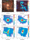 |
Fig. 1 JWST and ALMA maps of NGC 3256. Top-left: color image of NGC 3256 combining the NIRCam filters F150W (blue), F200W (green), and F335M (red). The latter contains the PAH3.3 µm band. The gray box marks the field of view of the ALMA CO(2–1) map (top-right panel) and the tilted gray rectangle is the NIRSpec field of view (middle and bottom row panels). Top-right: ALMA CO(2–1) 230.54 GHz zeroth moment map. The red ellipse represents the beam FWHM (0″.39 × 0″.37). The units of the image are Jy kms−1 beam−1. The crosses mark the northern and southern nuclei of NGC 3256 based on the 235 GHz continuum. Middle-left: NIRSpec 4.6 µm continuum map (see Sect. 3.1). The units are mJy pixel−1. Middle-right, bottom-left, and bottom-right: maps of the HI 7–5 4.65 µm, H2 0–0 S(9) 4.69 µm, and CO υ = 1–0 P(5) 4.71 µm transitions, respectively (see Sect. 3.1). The maps are in units of 10−16 erg s−1 cm−2 pixel−1. The crosses indicate the nuclear position determined from the 4.6 µm continuum peak. The circular apertures in the last panel are the regions used to extract the spectra of individual regions (Sect. 3.3). |
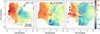 |
Fig. 2 Observed velocity fields of H I 7–5 4.65 µm (first panel), H2 0–0 S(9) 4.69 µm (second panel), and CO υ = 1–0 4.67 µm (third panel). The maps are in km s−1. |
Spectral features.
3 Analysis and results
In this paper, we focus on the rich 4.52–4.87 µm spectral range observed by JWST/NIRSpec where the rovibrational bands of 12CO (4.67 µm), 13CO (4.78 µm), and C18O (4.79 µm) are located. In addition to the CO bands, this spectral range also contains pure rotational and rovibrational H2 transitions as well as hydrogen recombination lines and ionized gas tracers. Table 1 shows the full list of spectral features used in this work.
To analyze the NIRSpec data cubes, we first produced spectral maps to extract the spatial information at the native NIRSpec resolution (~0″.2 at ~4.6 µm; Sects. 3.1 and 3.2). We then analyzed the spectra from selected regions of interest using larger apertures (0″.5 diameter; ~100 pc) to increase the signal-to-noise ratio (S/N; Sect. 3.3).
3.1 Mid-IR continuum, ionized, and molecular gas maps
We first produced spectral maps of various tracers in the spectral range around the 12CO band (4.59–4.75 µm) to trace the morphology and kinematics of the ionized and molecular gas phases and the mid-IR continuum (Figs. 1 and 2). To do so, we extracted the spectrum of each spaxel and fitted a model including the features listed in Table 1. For reference, Fig. 3 shows the annotated spectra of three regions of NGC 3256 (see Sect. 3.3 for details).
We fitted the local continuum level in the 4.59–4.75 µm range using a linear function. For the spectral features, we used Gaussian profiles. We tied the velocity and dispersion for groups of lines tracing the same phase of the gas: warm/hot molecular gas (H2 lines), and ionized gas (H I and [K III]4.62 µm). The relative velocity of the Dn-PAH band (Sect. 3.3.4) is tied to the H2 lines. The wavelength and width of the individual R- and P-branch CO transitions were also tied to a common line of sight velocity and velocity dispersion. In addition, the intensities of the H I lines were tied according to the expected case B ratios at 10 000 K (7–5/11–6 = 6.43; Storey & Hummer 1995). These two transitions are very close in wavelength (4.65 and 4.67 µm), and so the differential extinction is minimal and its effect on their ratio negligible. The intensity of the [K III]4.62 µm was tied to that of the H I 7–5 line because the former is fainter and blended with the CO R(5) transition. We estimated an average [K III]4.62 µm/H I 7–5 4.65 µm ratio of 0.104 in this object from the average ratio measured in regions with no CO R(5) detected. To create these maps, we omitted both the 13CO and C18O υ = 1–0 bands from the model because they are not blended with any of these H I or H2 transitions.
This spectral range contains numerous overlapping spectral features, and so to obtain an initial guess for the velocity and width of the lines in each spaxel, we used those derived from the H2 S(8) 5.05 µm and H I 10–6 5.13 µm lines, which are isolated in a less crowded spectral range.
From these fits, we obtained the intensity maps of the 4.6 µm continuum, the ionized gas traced by the H I 7–5 4.65 µm line, the molecular gas traced by H2 0–0 S(9) 4.69 µm, and the CO 1–0 P(5) transition, which is not strongly blended with other spectral features (see second and third rows of Fig. 1).
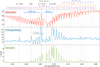 |
Fig. 3 Spectra of the CO υ = 1–0 band from the three classes defined in Sect. 3.2 (see Fig. 5) based on the absorption or emission of the P- and R-branches. The top panel shows the spectrum of the nuclear region where both branches are in absorption. The middle panel is the integrated spectrum of the regions where the R-branch is in absorption and the P-branch is in emission (rotating disk). The bottom panel is the integrated spectrum of areas with both branches in emission (outflow region perpendicular to the disk). The wavelengths of the P- and R-branches of the 12CO, 13CO, and C18O υ = 1–0 bands are marked by the dashed purple, orange, and blue lines, respectively. Transitions from other atomic and molecular species are marked by the dot-dashed black lines. The Dn-PAH band and the OCN− and CO ices are indicated in the middle and top panels. The rest frame is defined using the wavelength of the higher-J CO υ = 1–0 transitions detected, which for the nucleus are blueshifted with respect to the systemic velocity. |
3.1.1 Southern rotating disk. Ionized, molecular, and continuum emissions
In addition to the compact and bright 4.6 µm continuum and ionized gas emission from the southern nucleus (second row of Fig. 1), the southern disk is clearly seen extended along the east–west direction. The ionized gas is likely tracing star-forming regions in the disk, while the extended continuum is likely produced by hot dust heated by these star-forming regions.
The velocity field of the ionized gas traced by HI 7–5 4.65 µm (first panel of Fig. 2) is also consistent with a distorted rotating disk due to the galaxy interaction, and is compatible with previous near-IR kinematic studies of this system (Piqueras López et al. 2012). We note that the central ~ 100 pc velocity field is uncertain because the H2 and H I lines are heavily affected by the multi-component CO υ = 1–0 nuclear absorption (Sect. 3.2).
The hot (T > 1000 K) molecular gas traced by H2 0–0 S(9) 4.69 µm (Eup = 10261 K; Roueff et al. 2019) shows a more complex morphology (third row of Fig. 1). Some emitting regions are detected in the disk and the hot molecular gas kinematics also shows an east–west velocity gradient compatible with a distorted rotating disk (second panel of Fig. 2). However, the brightest hot molecular emission is located perpendicular to the rotating disk and is likely related to the massive molecular outflow (Emonts et al. 2014; Sect. 3.1.2).
3.1.2 Molecular outflow. H2 and CO emissions
The southern AGN produces a high-velocity (υ > 1000 km s−1) bipolar collimated molecular outflow perpendicular to the rotating disk (e.g., Sakamoto et al. 2014; Emonts et al. 2014). The hot molecular phase of this outflow has been detected using near-IR H2 transitions (Emonts et al. 2014). The H2 0–0 S(9) 4.69 µm emission also traces hot molecular gas and the emission perpendicular to the disk is likely related to this outflow (see Sect. 3.1.1). However, we note that due to the small field of view of NIR-Spec, the brightest hot H2 clumps of the outflow, which also have the highest velocity dispersion (σ ~ 190 km s−1; Emonts et al. 2014; Piqueras López et al. 2012), are not covered by these observations.
The cold molecular phase of the outflow is traced by the submm/mm rotational CO transitions (Sakamoto et al. 2014). The top row of Fig. 1 shows the morphology of the CO(2–1) 230.54 GHz transition. Although some CO(2–1) emission is detected in the southern disk, most of the emission around this nucleus is instead extended perpendicular to the disk up to ~400 pc away. Thanks to the high angular resolution of the ALMA data, it is clear that this emission is not part of the spiral arms of the northern galaxy and therefore it is likely located above and below the southern nucleus and its origin is likely connected to the molecular outflow. Consequently, we consider the emission from these regions to be part of the outflow. Moreover, the outflow direction is close to the plane of the sky (i ~ 80 deg; Sakamoto et al. 2014), and so even if the observed line-of-sight velocity is not particularly high (υ < 150 km s−1), the inclination corrected velocity can be much higher (see Sakamoto et al. 2014).
The bottom row of Fig. 1 presents the CO υ = 1–0 rovi-brational emission map as traced by the P(5) transition. It is similar to the CO(2–1) 230.54 GHz emission map, although the CO υ = 1–0 band is comparatively brighter in the outflow direction than in the disk emission (see Sect. 3.2). In Fig. 4, we compare the position–velocity (PV) plot along the outflow axis for the CO(2–1) and P(5) transitions. Excluding the strong nuclear absorption affecting the P(5) transition (Sect. 3.2), the two PV plots show a similar morphology. In particular, the higher-velocity blueshifted (−100 to −200 km s−1) outflow emission between −1″.l and −0″.3 is detected in both transitions. Therefore, based on the similar morphology and kinematics, we conclude that the rovibrational CO emission is related to the cold molecular outflow identified in the ALMA data.
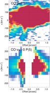 |
Fig. 4 Position–velocity cuts taken along the outflow axis (PA = 0°) of the CO(2–1) 230.54 GHz (top) and the CO υ = 1–0 P(5) 4.709 µm (bottom) transitions. For the CO(2–1), we used the spatially unsmoothed cube with a beam FWHM of 0″.23 × 0″.20. The nuclear P(5) absorption around the offset of ~0″ is masked in the bottom panel. Positive offsets are north of the nucleus. |
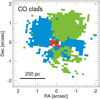 |
Fig. 5 Classification of the CO υ = 1–0 band according to the absorption or emission of the P- and R-branches. The red area marks regions with both branches in absorption. The blue area indicates regions where the R-branch is in absorption and the P-branch in emission. The green areas are regions with both branches in emission. The spectra of these areas are presented in Fig. 3. |
3.2 Origin of the rovibrational CO v = 1–0 band
The ratio between the P- and R-branch transitions of the CO υ = 1–0 band can be used to investigate the physical conditions of the molecular gas as traced by CO. The R(2) 4.641 µm and P(5) 4.709 µm transitions are not blended with other features, and so they are ideal for comparing the P- and R-branches. We fitted a Gaussian profile to these two lines with tied velocity and velocity dispersion. We leave the peak of the Gaussian free allowing for both absorption and emission profiles. The R(2) and P(5) transitions are detected in emission and absorption in different regions. According to the emission or absorption profiles, we classify the spaxels in three groups: (a) both transitions in absorption; (b) R(2) in absorption and P(5) in emission (P–R asymmetry); and (c) both transitions in emission. The integrated spectra of these regions are shown in Fig. 3 and the spatial classification in Fig. 5. It is clear from this map that (a) spaxels correspond to the nucleus where the strong 4.6 µm continuum favors the detection of the CO υ = 1–0 band in absorption. Also, we note that the nuclear CO υ = 1–0 spectrum has two velocity components: a low-velocity colder component only detected in the low-J transitions (up to J~6); and a blueshifted (v = l60 km s−1) possibly outflowing component detected up to J = 19. The (b) spaxels showing the P–R asymmetry are mostly located along the disk of the galaxy. This P–R asymmetry has been detected in Galactic star-forming regions (e.g., González-Alfonso et al. 2002, 1998), which is consistent with the spatial location of these regions in NGC 3256. Finally, the (c) spaxels with both P- and R-branches in emission are detected perpendicular to the disk in the molecular outflow region. The CO υ = 1–0 band can be radiatively excited by ~4.7 µm photons. Therefore, it is possible to explain this CO υ = 1–0 emission if the mid-IR radiation from the AGN is illuminating the cold molecular outflowing gas (see Fig. 6). This scenario and the method to derive the cold molecular gas properties from the CO υ = 1–0 band are further explored in Sects. 4 and 5.
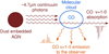 |
Fig. 6 Sketch showing how the CO ν = 1–0 band emission is produced in the outflow region of NGC 3256 S. The ~4.7 μm photons from the dust around the AGN (brown lines) illuminate the molecular clouds (blue ellipse). These photons are absorbed by CO molecules, which are excited to the ν = 1 levels and decay through the P- and R-branches (orange lines). The CO ν = 1-0 absorption is only observed in lines of sight that intersect both the ~4.7 μm continuum source and the molecular clouds. |
3.3 Spectra from regions with CO ν = 1–0 in emission
We extracted the spectra from eight circular apertures (0″.75 diameter) in the outflow region where both the P- and R-branches are detected in emission (green area in Fig. 5; see also Sect. 3.2). The location of these apertures is plotted in the bottom-right panel of Fig. 1. These apertures follow the outflow axis (N1, N2, and S1) and a few clumps seen in the CO ν = 1–0 map (Fig. 1 bottom right panel; N3, N4, N5, S2, and S3).
As the nuclear emission is compact and relatively bright (Fig. 1), we need to subtract its contribution to the spectrum of these apertures. We calculated this contribution at each wavelength using point-spread functions (PSFs) created with WebbPSF (v1.1.1; Perrin et al. 2014). These PSFs were rotated and convolved with a Gaussian kernel (FWHM = 0″ 130 × 0″.077) to match the orientation and FWHM of the southern nucleus of NGC 3256. Using these PSFs, we estimated the scaling factor between the emission at the aperture position and that from a fiducial aperture (0″.4 diameter) centered on the PSF. Using the fiducial aperture, we then measured the NGC 3256 S nuclear emission and applied the scaling factor to subtract its contribution to the aperture spectrum.
We fitted the spectral features in the 4.52–4.87 μm range following a procedure similar to that described in Sect. 3.1. However, because of the higher S/N of these spectra compared to the individual spaxel spectra, we used a more detailed model that includes additional spectral features and components. We describe the main elements of this more detailed model in Sects. 3.3.1 through 3.3.5.
3.3.1 Continuum baseline
The shape of the continuum around the CO ν = 1–0 rovibra-tional band can be affected by absorption bands produced by various ice species (OCN− 4.62 μm, 12CO 4.67 μm, and 13CO 4.78 μm; e.g., Gibb et al. 2004; McClure et al. 2023). To take into account these effects on the continuum shape, we defined a spline-interpolated baseline. The pivot points (4.395, 4.530, 4.586, 4.667, 4.845, and 4.980 μm) are selected to track the continuum level, avoiding known emission features. This baseline reproduces the underlying continuum and ice absorptions well (e.g., Fig. 7) and was subtracted from the spectra before fitting the emission lines.
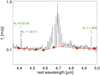 |
Fig. 7 Spectrum from region N3 (black line) and the spline-interpolated continuum baseline (red line). The pivot points are indicated by the red circles (see Sect. 3.3.1). The wavelengths of the three H2 transitions not presented in Figs. 3 and 8 are indicated in green (see also Table 1). |
3.3.2 Optically thin 13CO and C180 v= 1–0 bands
The R-branch of the 13CO and C18O ν = 1–0 bands overlaps with the P-branch of the 12CO band (see Fig. 3). Although, the 13CO and C18O bands are weaker than the band produced by the main isotopologue 12CO, for P-branch transitions with J > 8, the intensities of the overlapping R-branch transitions from the iso-topologues are comparable to or brighter than the 12CO lines. To disentangle the bands from the three species, we used Gaussian profiles to fit the P-branch and the R(0) transition of 13CO, which are not affected by 12CO band. The widths and velocities of these profiles were tied and we fitted them independently of the kinematic obtained for the 12CO band. The 13CO P(2)/R(0) ratio is consistent within ±1 σ with the optically thin limit, ~ 1.96 (see Sect. 4.1), for all the regions (except for S3 where the 13CO band spectral range is noisier).
Therefore, it is reasonable to assume that the 13CO (and also the C18O) emission is optically thin. Under this assumption, it is possible to determine the flux of the R-branch using the measured P-branch fluxes (Sect. 4.1). We estimated the intensity of the C18O band assuming that both 13CO and C18O share the same excitation temperatures and have an abundance ratio of ~7.4. We derived this abundance ratio from the 13CO(2−l)/C18O(2−l) ratio measured at the southern nucleus using a circular aperture (r = 1″). This abundance ratio agrees with that obtained by Harada et al. (2018) for the same region using a slightly larger aperture, of namely 5.6–6.6.
The model for the 13CO and C18O band emission is also subtracted from the spectra of the eight circular apertures before fitting the12 CO band. Under the optically thin limit, the fluxes predicted for the R-branch lines based on the P-branch observations agree with the observed spectra for all the regions including region S3 (Fig. 8).
3.3.3 Molecular hydrogen and recombination lines
There are two H2 transitions (0–0 S(9) 4.69 μm and 1–1 S(10) 4.66μm) and two HI recombination lines (7− 54.65 μm and 11−64.67 μm) that lie close to the center of the 12CO band. The fluxes of the S(9) 4.69 μm and 7−54.65 μm transitions are similar to the CO band fluxes, while the fluxes of the remaining two transitions are fainter.
In order to constrain the contribution of all these lines, we made use of additional H2 and HI recombination lines in the NIRSpec range (see Table 1). We determined the profile of the H2 lines by fitting a Gaussian (or two Gaussians when a single Gaussian cannot reproduce the observed profile) to the 0−0 S(8) 5.05 μm profile. For the 0−0 S(9) 4.69 μm transition, we used this profile, fixing its wavelength (velocity) and width (velocity dispersion) and allowing only the integrated flux to vary during the fit. The fainter 1−1 S(10) 4.66 μm is very close in wavelength to the CO R(0) and 7−5 transitions and so its flux is not well constrained. Therefore, we estimated its intensity assuming an excitation temperature equal to that derived from the 1−1 S(11) 4.42 μm and 1−1 S(9) 4.95 μm transitions and an ortho-to-para ratio of 3.
We fixed the velocity and width of the HI lines taking the HI 10−6 5.13 μm profile as reference. The integrated flux of the 7–5 transition is fitted, while for the 11–6 transition we assume the case B ratio (see Sect. 3.1).
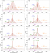 |
Fig. 8 Continuum-subtracted spectra (black line) of the selected regions (see Sect. 3.3 and bottom right panel of Fig. 1) where the CO v = 1−0 band is detected in emission. The red line is the best-fit model. The 13CO and C18O emission lines are fitted and subtracted (see Sect. 3.3.2) before fitting the remaining spectral features. The green, blue, and orange lines, which are also included in the best fit, represent the atomic and molecular transitions, the Dn-PAH feature, and the 13CO v = 1−0 band, respectively. The wavelengths of the 12CO v = 1−0 transitions are indicated in purple. All the spectral features present in the best-fit model are listed in Table 1. |
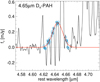 |
Fig. 9 Gaussian fit to the 4.65 μm Dn-PAH profile (red line). We masked the CO R-branch absorptions in the spectrum of the P-R asymmetry region (solid black line) so that only the blue circles are considered for this fit (see Sect. 3.3.4). |
3.3.4 The 4.65 μm Dn-PAH profile
The aliphatic C-D stretch in deuterated PAH (Dn-PAH) produces a broad band at ~4.65 μm. This band has been detected in Galactic sources and is predicted by quantum chemical computations (e.g., Peeters et al. 2004; Onaka et al. 2014; Doney et al. 2016; Buragohain et al. 2020; Yang & Li 2023). An accurate profile of this feature is not yet available due to the limited S/N and/or spectral resolution of these observations. Therefore, we determined the Dn-PAH profile from the observations of NGC 3256-S.
We used the spectrum from the P-R asymmetry region (middle panel of Fig. 3) where the low-J R-branch transitions of the CO v = 1−0 band are detected in absorption over the 4.65 μm Dn-PAH feature. We fit a Gaussian to the continuum-subtracted spectrum between 4.62 and 4.67 μm after masking the CO absorptions and the HI 7–5 and H2 1–1 S(10) transitions (Fig. 9). The redshift of this spectrum was determined using the H2 0–0 S(8) line as reference. The central wavelength of the best-fit Gaussian is 4.6452 ± 0.0004 ± 0.0014 μm where the uncertainties are statistical and due to the redshift, respectively. The width of this Gaussian profile is σ = 0.0091 ± 0.0003 μm The Dn-PAH band has been detected in Galactic sources using NIRSpec observations (Boersma et al. 2023). The central wavelength and width we obtained are compatible with the Galactic profile, although we note that they report a lower S/N for the band than in the spectrum analyzed here (5.25 vs. 11).
3.3.5 12CO v = 1−0 band
After subtracting the continuum baseline (Sect. 3.3.1) and the 13CO and C18O bands (Sect. 3.3.2), we fit the 12CO band together with the H2 and HI transitions (Sect. 3.3.3) and the 4.65 μm Dn-PAH band (Sect. 3.3.4), considering all the constraints described above.
We first attempted the fit using a single Gaussian profile for each CO transition. Two regions (N1 and N2) show a second broader kinematic component in the residuals. For these regions, we repeated the fit using two Gaussians for the CO band. We note that the fluxes of the broad component are not well constrained for the R(2) and R(3) transitions, which are close to the Dn-PAH band and the H I 7–5 transition. Therefore, we did not attempt to disentangle the fluxes of the narrow and broad components for these regions and only considered the integrated flux of the line.
The best-fit model for each region is shown in Fig. 8. From these fits, we obtained the fluxes of the P- and R-branch transitions (Table 2), which we used to calculate the ratios discussed in Sects. 4 and 5.
3.4 ALMA rotational 12CO emission
Using the ALMA observations of NGC 3256-S (Sect. 2.3), we measured the fluxes of the CO(1–0) 115.27 GHz and CO(2–1) 230.54GHz transitions in the selected regions (see Sect. 3.3). We extracted the spectra of the each region from the ALMA data cubes and integrated the line profile. The fluxes are listed in Table 3. We also calculated the r21 ratio between the fluxes of the CO(2–1) and CO(1–0) transitions in K km s−1 units.
4 Rovibrational CO v = 1−0 emission model
As mentioned in Sect. 3.2, in the outflow region of NGC 3256 S, the CO v = 1−0 emission can be excited by radiative pumping. The AGN is deeply dust embedded (Ohyama et al. 2015) and this dust absorbs and re-emits part of the AGN radiation in the mid-IR at ~4.7 μm This re-emitted light behaves as a lamp that directly illuminates molecular clouds above and below the disk and excites the v = 1 levels of CO through the absorption of ~4.7 μm continuum photons. The excited molecules then decay to the fundamental v = 0 levels emitting in the v = 1–0 P- and R-branches (see sketch in Fig. 6). For the P-branch transitions Jup − J10 = −1, while for the R-branch transitions Jup − J10 = +1, where J is the rotational quantum number.
Under this geometry every absorbed ~4.7 μm continuum photon results in the emission of a single P- or R-branch photon (according to the transition probabilities). In this case, the radiation field from the AGN is not intense enough to affect the excitation of the molecular cloud (see Sect. 4.2). Instead, the rovibrational CO emission acts as a probe of the physical conditions (temperature and column density) of the molecular gas in the illuminated clouds.
Here, we discuss ratios between P- and R-branch lines, which trace the physical conditions of the molecular gas when the CO band is detected in emission. We used in our analysis the CO molecular data from Goorvitch (1994) and the collisional coefficients from Yang et al. (2010).
4.1 The P(J+2)/R(J) ratio
We define the ratio between the P(J+2) and R(J) transitions as fJ = Fp(J+2)/FR(J), where F is the flux of each line. In this section, we determine the value of this ratio in the optically thin and thick limits and then we use nonlocal thermodynamic equilibrium (NLTE) models to determine its dependence on the CO column density (N(CO)), kinetic temperature (Tkin), and number density  .
.
4.1.1 Optically thin limit
In the optically thin limit, the flux of a transition is
 (1)
(1)
where Ω is the solid angle, h the Planck constant, Nup the column density of the upper level, and vul and Aul are the rest frequency and Einstein A-coefficient of the transition, respectively.
The P(J+2) and R(J) transitions share the same vibrationally excited upper level (vup = 1, Jup = J + 1). Their ratio therefore only depends on molecular constants:
 (2)
(2)
The gray crosses in Fig. 10 show the optically thin limit ratios. The observed ratios, shown by the filled red circles in the left panel of Fig. 10, clearly deviate from this limit.
Fluxes and velocity dispersion of the 12CO and 13CO v = 1−0 bands.
Fluxes of the 12CO rotational transitions.
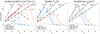 |
Fig. 10 Predicted P(J+2)/R(J) ≡ fJ ratios for the 12CO v = 1−0 band. The optically thin limit is represented by the gray crosses (Sect. 4.1.1). The black diamonds show the optically thick limit for three rotational temperatures (15, 25, and 35 K; Sect. 4.1.2). The dependence on N(CO)/σv (left panel), Tkin (middle panel), and |


4.1.2 Optically thick limit
Alternatively, if the CO rovibrational emission is optically thick, the flux of an emission line can be approximated by
 (3)
(3)
where c is the speed of light, 𝑔 is the level degeneracy, 2J + 1, of the upper and lower levels, N10 the column density of the lower level, and Δv is the width of the line. Therefore, the fJ ratio is connected to the level population of the ground (v = 0) CO states through the following relation (Sahai & Wannier 1985; González-Alfonso et al. 2002):
 (4)
(4)
where Nv,J is the population of the level with vibrational quantum number v and rotational quantum number J, and 𝑔J is the level degeneracy. In these equations, it is assumed that the population of the vibrationally excited levels (v = 1) is much smaller than that of the ground (v = 0) levels (N0,j/N1,J » 1), which is reasonable for cold molecular regions detached from the mid-IR continuum source that excites the CO rovibrational emission by radiative pumping.
Equation (4) contains the ratio between the v = 0 populations of the J and J + 2 levels, and so it is also possible to connect the  ratio and the excitation temperature, Trot(J, J + 2), within the v = 0 state:
 (5)
(5)
where Ev,J is the energy of the level with quantum numbers v and J. Figure 10 shows the optically thick limit for three temperatures (15–35 K; black lines) which, in a semi-log plot, is a straight line whose slope and (y-intercept depend on Trot.
For J < 4, the observed fJ (red circles in the left panel of Fig. 10) approximately follow a straight line, which indicates that these transitions are optically thick. For higher J, the observed ratios deviate from the optically thick limit toward the optically thin limit. This is expected given that N0,J, and the optical depth of the transitions are expected to decrease with increasing J for a sufficiently high J and a finite column density as in real molecular clouds.
4.1.3 NLTE models
We produced a grid of NLTE radiative transfer models to determine the dependence of the fJ ratios on Tkin and N(CO)/σv, where σv is the velocity dispersion, and the H2 density,  . First, we used RADEX (van der Tak et al. 2007) to determine the CO v = 0 level populations for Tkin between 12 and 50 K, N(CO)/σv between 10160 and 1020 cm−2/(km s−1), and
  between 102 and 106 cm−3 with 50 log steps for each parameter (125 000 models in total).
Then, the flux of each transition is derived from the following radiative transfer equations:
 (6)
(6)
 (7)
(7)
 (8)
(8)
 (9)
(9)
 (10)
(10)
where N and 𝑔 are the column density and degeneracy of the lower and upper levels of the transition, respectively, and Bv(TCMB) is the black body emission of the cosmic microwave background (CMB) at 2.73 K. The CMB emission does not affect the rovibrational band, but it is needed to calculate the emission of the CO rotational transitions in Sect. 5. We note that for the rovibrational transitions r − 1 ≃ r, because N10 » Nup. Equation (10) is the continuum-subtracted emission, which we integrated over frequencies to determine the intensities of the transitions.
By using these equations, we ignore line overlaps. The separation between the observed rovibrational transitions is > 470 km s−1 for J < 10, and so even for the broad outflow profiles (see Fig. 8), the effects of line overlapping are limited. In Eq. (10), we also ignore the term accounting for the mid-IR background continuum in our line of sight, because it has a low flux compared to that of the CO rovibrational lines.
For the v = 0 level populations, we used those calculated by RADEX, while for the v = 1 populations, we assumed that N1,J = k × N0,J, where k << 1 is a constant scaling factor. We note that k cancels out in the fj ratio, and so its actual value is not relevant. Radiative excitation slightly alters the excitation temperature of the v = 1 and v = 0 levels, and so the assumption N1,J = k × N0,J is not completely valid. However, when the excitation of the v = 0 levels is dominated by collisions (see Sect. 4.2), a grid of full radiative transfer models created using an updated version of the González-Alfonso et al. (1998) code indicates that this is an adequate approximation, because deviations are small for optically thick lines (<30%). For optically thin lines, the deviations are also small, resulting in rotational temperatures of the v = 1 levels that are 3–5 K higher than the rotational temperature of the v = 0 levels.
Figure 10 shows the fJ ratios predicted by these models. The first panel shows the dependence on N(CO)/σv for fixed Tkin and  . The ratios remain close to the optically thick limit up to a given J, which increases with increasing N(CO)/σv. This is because the optical depth of the transitions, τ, increases with N (CO)/σv
The middle panel of Fig. 10 shows the dependence on Tkin. For fixed N(CO)/σv and  , the low-J ratios (e.g., f0) increase with decreasing Tkin. Thus, the J at which the observed ratios deviate from the optically thick limit together with the low-J ratios can constrain both the CO column density and Tkin.
The dependence on  is presented in the right panel of Fig. 10. For
  , the fJ ratios have a positive curvature before reaching the maximum value. For
  , the ratios are almost equal to the LTE limit and are not sensitive to
  . This positive curvature is only observed in one of the regions studied here (N5), where it can help in constraining
  . However, in most cases, this curvature is not present and we can only estimate that their
  is larger than 103−4 cm−3. In Sect. 5, we use these NLTE models to estimate the CO-to-H2 conversion factor.
4.2 Collisions versus IR radiative pumping
In this section, we investigate whether or not the excitation of the pure rotational v = 0 levels of CO is affected by the IR radiative pumping in these regions as occurs for other molecules when the ratio between the intensity of the radiation and  is high enough (e.g., HNC and HCN; Aalto et al. 2007; Imanishi et al. 2017). The de-excitation of the v = 1 CO levels is dominated by the spontaneous emission of photons in the v = 1−0 band, which has much higher transition probabilities than the rotational transitions within two v = 1 levels. Moreover, the densities expected in molecular outflows are well below the critical density (
 at 160 K for collisions with H2; see González-Alfonso et al. 2002) of these transitions. Therefore, collisional and rotational de-excitation of the v = 1 levels can be neglected.
In this context, it is reasonable to assume that every absorbed ~4.7 μm continuum photon is re-emitted as a single photon in the v = 1−0 P- or R-branch. Therefore, assuming that the CO v = 1−0 emission is isotropic, we transformed the observed CO v = 1−0 fluxes (Table 2) into the rate of v = 1−0 emitted photons, that is, the IR radiative pumping rate RIR (e.g., González-Alfonso et al. 2022). We find the rates to be in the range (0.3−4.1) × 1051 s−1.
To estimate the rate of collisions, first we obtained the number of CO molecules, NCO, in each region from the CO(1–0) 115.27 GHz luminosity (Table 3) assuming an αCO factor and a CO abundance relative to H2, [CO/H2]. The rate of collisions is  , where γul are the collisional de-excitation coefficients with H2 for the lowest CO v = 0 rotational levels ((0.35−1.6) × 10−10 cm3 s−1; Yang et al. 2010).
We find that the ratio between the IR radiative pumping rate and the rate of collisions is
![Mathematical equation: $\eqalign{ & {{{R_{{\rm{IR}}}}} \over {{\gamma _{{\rm{ul}}}}{n_{{{\rm{H}}_2}}}{{\cal N}_{{\rm{CO}}}}}} = (0.2 - 5.8) \times {10^{ - 3}} \cr & \,\,\,\,\,\,\,\, \times {{0.8{M_ \odot }{{\left( {{\rm{Kkm}}{{\rm{s}}^{ - 1}}{\rm{p}}{{\rm{c}}^2}} \right)}^{ - 1}}} \over {{\alpha _{{\rm{CO}}}}}} \times {{{{10}^4}{\rm{c}}{{\rm{m}}^{ - 3}}} \over {{n_{{{\rm{H}}_2}}}}} \times {{3.2 \times {{10}^{ - 4}}} \over {\left[ {{\rm{CO}}/{{\rm{H}}_2}} \right]}}, \cr} $](/articles/aa/full_html/2024/01/aa47942-23/aa47942-23-eq31.png) (11)
(11)
Therefore, for the ULIRG-like αCO (0.8 M⊙ (K km s−1 pc2)−1; Bolatto et al. 2013) usually assumed for outflows, the excitation of the rotational CO levels is dominated by collisions for densities of  . Even if the αCO of outflows is down to a factor of two lower than the ULIRG-like factor (see Sect. 5), the contribution from radiative pumping to the rotational excitation of CO would be two times higher but still not dominant (<2%).
5 CO-to-H2 conversion factor
It is possible to determine the CO-to-H2 conversion factor (αCO = Mmol/LCO(1−0)) if the physical conditions of the gas are known, that is, Tkin and N(CO)/σv. Using Eqs. (6)–(10), we derived the integrated intensity, W(CO(1–0)), of the CO(1– 0) 115.27GHz transition in K km s−1. N(H2) is calculated as (N(CO)/σv) × σv/[CO/H2]. Then, the ratio N(H2)/W(CO(1−0)), known as XCO, is converted to αCO, multiplying the H2 mass by 1.36 to account for helium and other elements (Bolatto et al. 2013). Knowing the exact value of σv is not critical, because in the optically thick limit, W(CO(1−0)) ∝ Tb × σv, where Tb is the peak brightness temperature, and so it cancels out in the XCO definition.
We discuss three different methods to measure αCO using the CO v = 1−0 band. We used a single-component NLTE model (see Sect. 4.1.3) to fit the P(J+2)/R(J) ratios (Sect. 5.1). This single-component model fails to reproduce the higher-J ratios, and so we included a second component in Sect. 5.2. Finally, for the regions where the 13CO v = 1−0 band is well detected, we used it to constrain the excitation temperature of the 12CO v = 0 levels (Sect. 5.3).
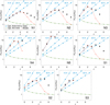 |
Fig. 11 Ratio between the P(J+2) and R(J) transitions of the CO v =1−0 band for the selected regions (black circles). The best-fit single-component model is represented by the red empty squares (see Sect. 5.1). The parameters of the best-fit models are listed in Table 4. The blue diamonds and green crosses show the optically thick and thin limits, respectively (see Sects. 4.1.1 and 4.1.2). The points are connected by lines to guide the eye. |
5.1 Single-component model
Figure 11 shows the best-fit for each region using a single NLTE model. A single component is not able to simultaneously reproduce the low- and high-J P(J+2)/R(J) ratios. We focus on fitting the low-J transitions, because these are likely tracing the bulk of the molecular gas mass.
The higher-J ratio used in the fit for each region is set as the maximum J that can be reproduced by a single-component model (i.e., when χ2 does not significantly increase when adding that ratio). This single-component model can fit between four and six ratios. The physical conditions of the gas derived for each region are listed in Table 4.
Tkin varies between 14 and 35 K. For these regions, we find a temperature gradient with decreasing Tkin at further distances from the nucleus. To investigate this gradient, we created a 2D map of rotational temperature using the f0 ratio measured in each spaxel (Sect. 3.1) assuming the optically thick limit (Eq. (4)). In this limit, the rotational temperature is equal to Tkin if the low-J levels are thermalized. Figure 12 clearly shows, especially at the northern outflow region, that the molecular gas cools down from >40 K at the central 100 pc to < 15 K at ~250 pc. This result is also consistent with the low kinetic temperature (~9 K) in the molecular outflow compared to the nuclear gas temperature (~40 K) measured in the LIRG ESO 320-G030 at similar spatial scales (Pereira-Santaella et al. 2020).
The number density  is not well constrained in general, with lower limits of around 102.5–4 cm−3. N(CO)/σv is better constrained and varies between >1016.9 and 1018.0 cm−2 (km s−1)−1.
From these physical conditions, we also calculated the αCO conversion factor as described above in Sect. 5. We find αCO in the range of ![Mathematical equation: $(0.26 - 0.53) \times {{3.2 \times {{10}^{ - 4}}} \over {\left[ {{\rm{CO}}/{{\rm{H}}_2}} \right]}}{M_ \odot }$](/articles/aa/full_html/2024/01/aa47942-23/aa47942-23-eq34.png) (K km s−1 pc2)−1 with a median (mean) of 0.40 ± 0.15 (0.50 ± 0.30). This is about ten times lower than the Galactic αCO (4.3 M⊙ (K km s−1 pc2)−1; e.g., Bolatto et al. 2013), and also about two times lower than the ULIRG αCO (0.8 M⊙ (K km s−1 pc2)−1), which is typically used to estimate the mass of cold molecular outflows (e.g., Cidone et al. 2014; Fiore et al. 2017; Pereira-Santaella et al. 2018; Lutz et al. 2020; Lamperti et al. 2022).
(K km s−1 pc2)−1 with a median (mean) of 0.40 ± 0.15 (0.50 ± 0.30). This is about ten times lower than the Galactic αCO (4.3 M⊙ (K km s−1 pc2)−1; e.g., Bolatto et al. 2013), and also about two times lower than the ULIRG αCO (0.8 M⊙ (K km s−1 pc2)−1), which is typically used to estimate the mass of cold molecular outflows (e.g., Cidone et al. 2014; Fiore et al. 2017; Pereira-Santaella et al. 2018; Lutz et al. 2020; Lamperti et al. 2022).
It is also common to observe alternative low-J CO rotational transitions, such as the 2−1 or the 3−2 at 230.54 and 345.80 GHz, respectively, instead of the CO(1−0). In these cases, the observed flux must be converted to an equivalent CO(1−0) flux before using the αCO factor by assuming a CO(2−1) to CO(1−0) ratio (r21) or CO(3−2) to CO(1−0) ratio (r32). From the models, we also determined the expected r21 and r31 ratios. The mean ratios are 1.08 ± 0.09 and 0.97 ± 0.16, respectively. The measured r21 in the outflow regions are between 0.69 and 1.14 (Table 3), with a mean ratio of 0.88 ± 0.15, which is in good agreement with the models.
Single-component models.
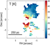 |
Fig. 12 Rotational temperature of the molecular gas derived from the ratio between the CO v = 1−0 P(2) and R(0) transitions assuming the optically thick limit (Eq. (4)). Only positions where both the R- and P- branches are in emission are considered. The black cross marks the position of the southern nucleus of NGC 3256. |
5.2 Two-component model
The single component models are not able to reproduce all the fJ ratios simultaneously. In this section, we add a second component to the models of regions with six or more fJ ratios detected where a single component clearly fails to reproduce the observations. To find the best-fit model, we calculated the χ2 for all the possible combinations of two models of the grid, leaving only a scaling factor between the two models (ratio between their solid angles) as a free parameter. To limit the number of combinations, we only considered three number densities, of 103, 104, and 105 cm−3, given that the CO v = 1−0 band is not very sensitive to  . In total, we explored 56 million combinations of models for each region.
The best-fit models are shown in Fig. 13. With two components, it is now possible to fit all the observed ratios. To determine the likelihood function of the parameters, we assigned a probability to each model of exp(−χ2/2) and then calculated the marginalized likelihoods for each parameter. The parameter values are listed in Table 5. We find that the best-fit models include a “cold” (Component 1) with a mean Tkin of 17 K, and a “warmer” component (Component 2) with a mean Tkin of 30 K. The N(CO)/σv of the cold component is ~1018.0 cm−2 (km s−1)−1 which is ~0.2 dex higher than that of the warm component. We calculated the αCO weighted by the intensity of the CO(1−0) 115.27 GHz intensity of each component. The αCO are in the range of ![Mathematical equation: $(0.5 - 0.7) \times {{3.2 \times {{10}^{ - 4}}} \over {\left[ {{\rm{CO}}/{{\rm{H}}_2}} \right]}}{M_ \odot }$](/articles/aa/full_html/2024/01/aa47942-23/aa47942-23-eq38.png) (K km s−1 pc2)−1 with a median value of 0.61 ± 0.17. These αCO are 1.3–2.3 times higher than the αCO derived using a single-component model for the individual regions. The median ratio is more than seven times lower than the Galactic αCO, and slightly lower (~30%) than the ULIRG-like αCO. We find that the r21 and r31 ratios are consistent, within the uncertainties, with those derived using a single-component model (Sect. 5.1).
(K km s−1 pc2)−1 with a median value of 0.61 ± 0.17. These αCO are 1.3–2.3 times higher than the αCO derived using a single-component model for the individual regions. The median ratio is more than seven times lower than the Galactic αCO, and slightly lower (~30%) than the ULIRG-like αCO. We find that the r21 and r31 ratios are consistent, within the uncertainties, with those derived using a single-component model (Sect. 5.1).
5.3 Optically thin 13CO v= 1−0 band
The P–R line ratio f0 indicates that the 13CO v = 1−0 band is optically thin (Sect. 3.3.2), and therefore it can be used to estimate the mass of the molecular clouds in a similar way to the standard method for the submm/mm 13CO rotational transitions (e.g., Papadopoulos et al. 2012).
From Eq. (1), for 13CO in the optically thin limit, the population of the upper level is:
 (12)
(12)
For 12CO in the optically thick limit, using Eq. (3) we find
 (13)
(13)
Therefore, assuming that Ω and the excitation temperature of the v =1 and v = 0 levels is the same for 12CO and 13CO, the ratio between Eqs. (12) and (13) gives for the left-hand side of the ratio ![Mathematical equation: $\left( {N_{{\rm{lo}}}^{^{12}{\rm{CO}}}/{\rm{\Delta v}}} \right)/\left[ {^{12}{\rm{CO}}{/^{13}}{\rm{CO}}} \right]$](/articles/aa/full_html/2024/01/aa47942-23/aa47942-23-eq47.png) . From the 13CO and 12CO R(0) transitions, we estimate
. From the 13CO and 12CO R(0) transitions, we estimate  . To determine the intensity of the CO(1−0) 115.27 GHz transition using Eqs. (6)–(10), we need the population of the
  level, which we estimated based on the excitation temperature of the low-J levels – which ranges from 15 to 30 K – of the regions derived in Sect. 5.1 (see also Table 4 and Fig. 12). The population of the remaining
  levels is also estimated using the Sect. 5.1 excitation temperatures. We also need to transform the observed Δv (FWHM) into the σv used in Eq. (6). To do this, we first divided Δv by ~2.355 in order to account for the ratio between FWHM and σ. The observed Δv also depends on the optical depths of the 12CO v = 1−0 transitions, which are unknown. To account for this uncertainty, we divided Δv by an extra factor of between 1.2 and 2.6 (valid for τ between 1 and 100).
Then, estimating Mmol as described at the beginning of Sect. 5, we derived the αCO conversion factor for these eight regions (Table 6). The αCO values are found within the range of ![Mathematical equation: $(0.15 - 0.59) \times {{3.2 \times {{10}^{ - 4}}} \over {\left[ {{\rm{CO}}/{{\rm{H}}_2}} \right]}} \times {{\left[ {^{12}{\rm{CO}}{/^{13}}{\rm{CO}}} \right]} \over {60}}{M_ \odot }$](/articles/aa/full_html/2024/01/aa47942-23/aa47942-23-eq52.png) (K km s−1 pc2)−1 with a median range of 0.19–0.36. The median αCO are 1.1–2.1 times lower than those derived using the single-component NLTE model (Sect. 5.1) and 1.7-3.2 times lower than those obtained from the two-component models (Sect. 5.2). These αCO derived from 13CO are also more than 2 and 10 times lower than the ULIRG-like and Galactic αCO factors, respectively. We note that the αCO derived using the 13CO band depend on the 12CO abundance and the 13CO to 12CO abundance ratio in the outflow, which are both uncertain. Therefore, these αCO are more uncertain than those derived using the single- and two-component methods (Sects. 5.1 and 5.2), which only depend on the 12CO abundance.
(K km s−1 pc2)−1 with a median range of 0.19–0.36. The median αCO are 1.1–2.1 times lower than those derived using the single-component NLTE model (Sect. 5.1) and 1.7-3.2 times lower than those obtained from the two-component models (Sect. 5.2). These αCO derived from 13CO are also more than 2 and 10 times lower than the ULIRG-like and Galactic αCO factors, respectively. We note that the αCO derived using the 13CO band depend on the 12CO abundance and the 13CO to 12CO abundance ratio in the outflow, which are both uncertain. Therefore, these αCO are more uncertain than those derived using the single- and two-component methods (Sects. 5.1 and 5.2), which only depend on the 12CO abundance.
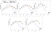 |
Fig. 13 Ratio between the P(J+2) and R(J) transitions of the CO v = 1−0 band for the selected regions ( filled black circles). The best-fit two-component model is shown as empty red squares (see Sect. 5.2). The blue and green empty squares represent components 1 (“cold”) and 2 (“warmer”) of the best-fit model, respectively. The parameters of the best-fit model are listed in Table 5. The points are connected by lines to guide the eye. |
Two-component models.
13CO models.
6 Discussion
We find that the αCO factors in the molecular outflow are 1.3–2 times lower than the ULIRG conversion factor and 6–8 times lower than the Galactic factor (assuming [CO/H2] = 3.2×10⁻⁴; Sect. 5). Below, we discuss several options to explain the origin of this reduced αCO in outflows.
For individual molecular clouds, the existence of an αCO factor, which relates the total molecular mass and the luminosity of the CO(1−0) 115.27 GHz line, relies on several assumptions: (1) the CO(1−0) emission is optically thick; (2) the molecular clouds are virialized; and (3) the mass is dominated by H2 (see e.g., Bolatto et al. 2013). Under these conditions
 (14)
(14)
All these assumptions seem to be valid for molecular clouds in the Milky Way and nearby spiral galaxies, where αCO = 3.1−4.3 M⊙ (K km s−1 pc2)−1 (e.g., Sandstrom et al. 2013; Bolatto et al. 2013). The temperatures (15–40 K) and densities (> 103 cm−3) we measured in the molecular outflow do not significantly differ from those observed in the molecular clouds found in disks. Therefore, the  and Tkin dependencies shown in Eq. (14) would not explain the low αCO in the outflow.
Dasyra et al. (2016) found that the rotational CO emission in the jet-driven outflow of IC 5063 is optically thin, and so αCO reaches a lower limit of 0.11 M⊙(K km s−1 pc2)−1 (for Tex = 30 K and [CO/H2] = 3.2×10⁻⁴). However, this explanation does not work for NGC 3256-S, because the CO emission from the outflow is optically thick.
The lower αCO of ULIRGs (0.8 M⊙(K km s−1 pc2)−1; Downes & Solomon 1998) is explained because the molecular clouds of these interacting or merging systems are not virialized and the width of the line is affected by large-scale motions and turbulence. This argument fits well with the conditions in outflows where the clouds are not self-gravitating (e.g., Pereira-Santaella et al. 2020). This increased velocity dispersion of the clouds increases the observed flux for optically thick lines (as in this outflow) and this results in a reduced αCO factor for the outflow.
We derived an αCO factor that depends on the [CO/H2] abundance ratio. The CO abundance in molecular outflows has not yet been firmly established, and so this is a major uncertainty for these results. We assumed a standard CO abundance of 3.2 × 10⁻⁴ (e.g., Bolatto et al. 2013), but CO might be dissociated in molecular outflows and become C I (Cidone et al. 2018; Saito et al. 2022). If so, our αCO values would increase. However, we note that it is not possible to accurately quantify the CO to C I dissociation in outflows. The [C I] emission is optically thin (e.g., Papadopoulos & Greve 2004), and so the total molecular mass, including molecular gas without CO, derived from its emission depends on the assumed [C I/H2] abundance ratio, which is also uncertain for outflows.
7 Summary and conclusions
We studied the spatially resolved 12CO v = 1−0 and 13CO v = 1−0 bands at 4.67 and 4.78 µm, respectively, around the dust-embedded AGN in the southern nucleus of NGC 3256. We modeled the ratios between the P(J+2) and R(J) transitions of the CO v = 1−0 emission using an NLTE approximation. Using these models, we constrained the column density, kinetic temperature, and αCO conversion factor of the cold molecular gas in the outflow. The main results of the paper can be summarized as follows:
- 1
CO band classification. Based on the detection in absorption or emission of the P- and R-branches of the CO v = 1−0 band, we classify the observed spectra into three categories: (a) both branches in absorption seen basically toward the mid-IR bright nucleus; (b) P–R asymmetry (i.e., P-branch in emission and R-branch in absorption) detected along the disk of the galaxy; and (c) both branches in emission detected above and below the disk in the outflow region. We focused on the latter in order to determine the physical conditions of the cold molecular gas in this AGN-launched outflow.
- 2
Origin of the CO v = 1−0 band emission. Detecting the band in emission can be explained as follows: the radiation from the deeply embedded AGN is reprocessed by dust that emits intense mid-IR ~4.7 µm continuum radiation. This continuum illuminates the molecular clouds in the outflow and excites the vibrational levels of CO, resulting in the v = 1−0 bands seen in emission in our line of sight.
- 3
Temperature gradient in the outflow. From the spatially resolved map of the 12CO v = 1−0 P(2)/R(0) ratio, we identify a temperature gradient in the outflow from >40 K in the central 100 pc to <15 K at 250 pc. This temperature gradient is similar to that found in the molecular outflow of the local LIRG ESO 320-G030 (Pereira-Santaella et al. 2020).
- 4
Reduced αCO in the outflow. We derived the αCO conversion factor in the outflow by fitting the observed P(J+2)/R(J) ratios in eight 100 pc (0″.5) apertures in the outflow region. We used three different approaches (single NLTE component, two NLTE components, and 13CO models). We find αCO within the range of
![Mathematical equation: $(0.26 - 1.09) \times {{3.2 \times {{10}^{ - 4}}} \over {\left[ {{\rm{CO}}/{{\rm{H}}_2}} \right]}}\quad {M_ \odot }$](/articles/aa/full_html/2024/01/aa47942-23/aa47942-23-eq55.png) (K km s−1 pc2)−1 for the NLTE modeling with median values of 0.40 ± 0.15 and 0.61 ± 0.17 for the single- and two-component models, respectively. These are 1.3–2 times lower than the ULIRG-like αCO typically assumed for outflows. From the 13CO models, we find a median
(K km s−1 pc2)−1 for the NLTE modeling with median values of 0.40 ± 0.15 and 0.61 ± 0.17 for the single- and two-component models, respectively. These are 1.3–2 times lower than the ULIRG-like αCO typically assumed for outflows. From the 13CO models, we find a median ![Mathematical equation: ${\alpha _{{\rm{CO}}}} = (0.19 - 0.36) \times {{3.2 \times {{10}^{ - 4}}} \over {\left[ {{\rm{CO}}/{{\rm{H}}_2}} \right]}} \times {{\left. {^{[12}{\rm{CO}}{/^{13}}{\rm{CO}}} \right]} \over {60}}{M_ \odot }$](/articles/aa/full_html/2024/01/aa47942-23/aa47942-23-eq56.png) (K km s−1 pc2)−1, which is lower than those derived from the NLTE models, although it is subject to the uncertain [12CO/13CO] abundance ratio in the outflow. The most likely explanation for this reduced αCO is that the molecular clouds in the outflow are not virialized.
(K km s−1 pc2)−1, which is lower than those derived from the NLTE models, although it is subject to the uncertain [12CO/13CO] abundance ratio in the outflow. The most likely explanation for this reduced αCO is that the molecular clouds in the outflow are not virialized. - 5
Dn-PAH detection. We detected a broad (σ = 0.0091 ± 0.0003 µm) spectral feature at 4.645 ± 0.002 µm, which is produced by the aliphatic C-D stretch mode in deuterated PAH (Dn-PAH). The Dn-PAH emission is detected in the disk of the galaxy and also in the apertures selected in the outflow, although the latter could be background or foreground emission not directly connected to the outflow.
- 6
Optically thick 12CO emission in the outflow. The observed ratios indicate that the 12CO v = 1−0 emission is optically thick, at least for J < 4, while the 13CO v = 1−0 emission remains optically thin.
Establishing the αCO factor of outflows is important in order to transform the high-velocity rotational CO emission routinely observed in both nearby and high-z galaxies into accurate mass-outflow rates. We showed that the CO v = 1−0 ~4.67 µm band emission observed by JWST can be used to determine the physical conditions of the cold molecular gas in outflows and to constrain the αCO factor.
References
- Aalto, S., Spaans, M., Wiedner, M. C., & Hüttemeister, S. 2007, A&A, 464, 193 [NASA ADS] [CrossRef] [EDP Sciences] [Google Scholar]
- Alonso-Herrero, A., Pereira-Santaella, M., Rieke, G. H., & Rigopoulou, D. 2012, ApJ, 744, 2 [Google Scholar]
- Alonso-Herrero, A., Pereira-Santaella, M., García-Burillo, S., et al. 2018, ApJ, 859, 144 [Google Scholar]
- Alonso-Herrero, A., García-Burillo, S., Pereira-Santaella, M., et al. 2019, A&A, 628, A65 [NASA ADS] [CrossRef] [EDP Sciences] [Google Scholar]
- Alonso-Herrero, A., García-Burillo, S., Pereira-Santaella, M., et al. 2023, A&A, 675, A88 [NASA ADS] [CrossRef] [EDP Sciences] [Google Scholar]
- Baba, S., Nakagawa, T., Isobe, N., & Shirahata, M. 2018, ApJ, 852, 83 [NASA ADS] [CrossRef] [Google Scholar]
- Baba, S., Imanishi, M., Izumi, T., et al. 2022, ApJ, 928, 184 [NASA ADS] [CrossRef] [Google Scholar]
- Boersma, C., Allamandola, L. J., Esposito, V. J., et al. 2023, ApJ, 959, 74 [NASA ADS] [CrossRef] [Google Scholar]
- Böker, T., Arribas, S., Lützgendorf, N., et al. 2022, A&A, 661, A82 [NASA ADS] [CrossRef] [EDP Sciences] [Google Scholar]
- Bolatto, A. D., Wolfire, M., & Leroy, A. K. 2013, ARA&A, 51, 207 [CrossRef] [Google Scholar]
- Buragohain, M., Pathak, A., Sakon, I., & Onaka, T. 2020, ApJ, 892, 11 [NASA ADS] [CrossRef] [Google Scholar]
- Cidone, C., Maiolino, R., Sturm, E., et al. 2014, A&A, 562, A21 [NASA ADS] [CrossRef] [EDP Sciences] [Google Scholar]
- Cidone, C., Severgnini, P., Papadopoulos, P. P., et al. 2018, ApJ, 863, 143 [NASA ADS] [CrossRef] [Google Scholar]
- Combes, F., García-Burillo, S., Braine, J., et al. 2013, A&A, 550, A41 [NASA ADS] [CrossRef] [EDP Sciences] [Google Scholar]
- Dasyra, K. M., Combes, F., Oosterloo, T., et al. 2016, A&A, 595, L7 [NASA ADS] [CrossRef] [EDP Sciences] [Google Scholar]
- Díaz-Santos, T., Alonso-Herrero, A., Colina, L., et al. 2010, ApJ, 711, 328 [CrossRef] [Google Scholar]
- Doney, K. D., Candian, A., Mori, T., Onaka, T., & Tielens, A. G. G. M. 2016, A&A, 586, A65 [NASA ADS] [CrossRef] [EDP Sciences] [Google Scholar]
- Downes, D., & Solomon, P. M. 1998, ApJ, 507, 615 [NASA ADS] [CrossRef] [Google Scholar]
- Emonts, B. H. C., Piqueras-López, J., Colina, L., et al. 2014, A&A, 572, A40 [EDP Sciences] [Google Scholar]
- Feudhtgruber, H., Lutz, D., Beintema, D. A., et al. 1997, ApJ, 487, 962 [NASA ADS] [CrossRef] [Google Scholar]
- Fiore, F., Feruglio, C., Shankar, F., et al. 2017, A&A, 601, A143 [NASA ADS] [CrossRef] [EDP Sciences] [Google Scholar]
- García-Bernete, I., Alonso-Herrero, A., García-Burillo, S., et al. 2021, A&A, 645, A21 [EDP Sciences] [Google Scholar]
- García-Burillo, S., Combes, F., Usero, A., et al. 2015, A&A, 580, A35 [Google Scholar]
- Geballe, T. R., Goto, M., Usuda, T., Oka, T., & MdCall, B. J. 2006, ApJ, 644, 907 [NASA ADS] [CrossRef] [Google Scholar]
- Gibb, E. L., Whittet, D. C. B., Boogert, A. C. A., & Tielens, A. G. G. M. 2004, ApJS, 151, 35 [NASA ADS] [CrossRef] [Google Scholar]
- González-Alfonso, E., Cernicharo, J., van Dishoeck, E. F., Wright, C. M., & Heras, A. 1998, ApJ, 502, L169 [CrossRef] [Google Scholar]
- González-Alfonso, E., Wright, C. M., Cernicharo, J., et al. 2002, A&A, 386, 1074 [NASA ADS] [CrossRef] [EDP Sciences] [Google Scholar]
- González-Alfonso, E., Fischer, J., Goicoechea, J. R., et al. 2022, A&A, 666, L3 [NASA ADS] [CrossRef] [EDP Sciences] [Google Scholar]
- Goorvitch, D. 1994, ApJS, 95, 535 [NASA ADS] [CrossRef] [Google Scholar]
- Harada, N., Sakamoto, K., Martín, S., et al. 2018, ApJ, 855, 49 [Google Scholar]
- Harrison, C. M., Costa, T., Tadhunter, C. N., et al. 2018, Nat. Astron., 2, 198 [Google Scholar]
- Herczeg, G. J., Brown, J. M., van Dishoeck, E. F., & Pontoppidan, K. M. 2011, A&A, 533, A112 [NASA ADS] [CrossRef] [EDP Sciences] [Google Scholar]
- Imanishi, M., Nakanishi, K., & Izumi, T. 2017, ApJ, 849, 29 [NASA ADS] [CrossRef] [Google Scholar]
- Jakobsen, P., Ferruit, P., Alves de Oliveira, C., et al. 2022, A&A, 661, A80 [NASA ADS] [CrossRef] [EDP Sciences] [Google Scholar]
- Lamperti, I., Pereira-Santaella, M., Perna, M., et al. 2022, A&A, 668, A45 [NASA ADS] [CrossRef] [EDP Sciences] [Google Scholar]
- Leitherer, C., Chandar, R., Tremonti, C. A., Wofford, A., & Schaerer, D. 2013, ApJ, 772, 120 [NASA ADS] [CrossRef] [Google Scholar]
- Lira, P., Ward, M., Zezas, A., Alonso-Herrero, A., & Ueno, S. 2002, MNRAS, 330, 259 [CrossRef] [Google Scholar]
- Lira, P., Gonzalez-Corvalan, V., Ward, M., & Hoyer, S. 2008, MNRAS, 384, 316 [NASA ADS] [CrossRef] [Google Scholar]
- Lutz, D., Sturm, E., Janssen, A., et al. 2020, A&A, 633, A134 [NASA ADS] [CrossRef] [EDP Sciences] [Google Scholar]
- McClure, M. K., Rocha, W. R. M., Pontoppidan, K. M., et al. 2023, Nat. Astron., 7, 431 [NASA ADS] [CrossRef] [Google Scholar]
- McMullin, J. P., Waters, B., Schiebel, D., Young, W., & Golap, K. 2007, ASP Conf. Ser., 376, 127 [Google Scholar]
- Michiyama, T., Iono, D., Sliwa, K., et al. 2018, ApJ, 868, 95 [Google Scholar]
- Najita, J., Carr, J. S., & Mathieu, R. D. 2003, ApJ, 589, 931 [NASA ADS] [CrossRef] [Google Scholar]
- Ohyama, Y., Terashima, Y., & Sakamoto, K. 2015, ApJ, 805, 162 [Google Scholar]
- Ohyama, Y., Onishi, S., Nakagawa, T., et al. 2023, ApJ, 951, 87 [NASA ADS] [CrossRef] [Google Scholar]
- Onaka, T., Mori, T. I., Sakon, I., et al. 2014, ApJ, 780, 114 [Google Scholar]
- Onishi, S., Nakagawa, T., Baba, S., et al. 2021, ApJ, 921, 141 [NASA ADS] [CrossRef] [Google Scholar]
- Papadopoulos, P. P., & Greve, T. R. 2004, ApJ, 615, L29 [Google Scholar]
- Papadopoulos, P. P., van der Werf, P., Xilouris, E., Isaak, K. G., & Gao, Y. 2012, ApJ, 751, 10 [Google Scholar]
- Peeters, E., Allamandola, L. J., Bauschlicher, C. W. J., et al. 2004, ApJ, 604, 252 [NASA ADS] [CrossRef] [Google Scholar]
- Pereira-Santaella, M., Alonso-Herrero, A., Rieke, G. H., et al. 2010, ApJS, 188, 447 [NASA ADS] [CrossRef] [Google Scholar]
- Pereira-Santaella, M., Alonso-Herrero, A., Santos-Lleo, M., et al. 2011, A&A, 535, A93 [NASA ADS] [CrossRef] [EDP Sciences] [Google Scholar]
- Pereira-Santaella, M., Colina, L., García-Burillo, S., et al. 2018, A&A, 616, A171 [NASA ADS] [CrossRef] [EDP Sciences] [Google Scholar]
- Pereira-Santaella, M., Colina, L., García-Burillo, S., et al. 2020, A&A, 643, A89 [NASA ADS] [CrossRef] [EDP Sciences] [Google Scholar]
- Pereira-Santaella, M., Colina, L., García-Burillo, S., et al. 2021, A&A, 651, A42 [NASA ADS] [CrossRef] [EDP Sciences] [Google Scholar]
- Perrin, M. D., Sivaramakrishnan, A., Lajoie, C.-P., et al. 2014, SPIE Conf. Ser., 9143, 91433X [NASA ADS] [Google Scholar]
- PiquerasLópez, J., Colina, L., Arribas, S., Alonso-Herrero, A., & Bedregal, A. G. 2012, A&A, 546, A64 [NASA ADS] [CrossRef] [EDP Sciences] [Google Scholar]
- Ramos Almeida, C., Bischetti, M., García-Burillo, S., et al. 2022, A&A, 658, A155 [NASA ADS] [CrossRef] [EDP Sciences] [Google Scholar]
- Rettig, T. W., Brittain, S. D., Gibb, E. L., Simon, T., & Kulesa, C. 2005, ApJ, 626, 245 [NASA ADS] [CrossRef] [Google Scholar]
- Roueff, E., Abgrall, H., Czachorowski, P., et al. 2019, A&A, 630, A58 [NASA ADS] [CrossRef] [EDP Sciences] [Google Scholar]
- Sahai, R., & Wannier, P. G. 1985, ApJ, 299, 424 [NASA ADS] [CrossRef] [Google Scholar]
- Saito, T., Takano, S., Harada, N., et al. 2022, ApJ, 935, 155 [NASA ADS] [CrossRef] [Google Scholar]
- Sakamoto, K., Aalto, S., Combes, F., Evans, A., & Peck, A. 2014, ApJ, 797, 90 [Google Scholar]
- Sánchez-García, M., Pereira-Santaella, M., García-Burillo, S., et al. 2022, A&A, 659, A102 [NASA ADS] [CrossRef] [EDP Sciences] [Google Scholar]
- Sandstrom, K. M., Leroy, A. K., Walter, F., et al. 2013, ApJ, 777, 5 [Google Scholar]
- Shirahata, M., Nakagawa, T., Usuda, T., et al. 2013, PASJ, 65, 5 [NASA ADS] [CrossRef] [Google Scholar]
- Somerville, R. S., & Davé, R. 2015, ARA&A, 53, 51 [Google Scholar]
- Spoon, H. W. W., Moorwood, A. F. M., Pontoppidan, K. M., et al. 2003, A&A, 402, 499 [NASA ADS] [CrossRef] [EDP Sciences] [Google Scholar]
- Spoon, H. W. W., Armus, L., Cami, J., et al. 2004, ApJS, 154, 184 [NASA ADS] [CrossRef] [Google Scholar]
- Storey, P. J., & Hummer, D. G. 1995, MNRAS, 272, 41 [NASA ADS] [CrossRef] [Google Scholar]
- Ueda, J., Michiyama, T., Iono, D., Miyamoto, Y., & Saito, T. 2022, PASJ, 74, 407 [NASA ADS] [CrossRef] [Google Scholar]
- van der Tak, F. F. S., Black, J. H., Schöier, F. L., Jansen, D. J., & van Dishoeck, E. F. 2007, A&A, 468, 627 [NASA ADS] [CrossRef] [EDP Sciences] [Google Scholar]
- Veilleux, S., Maiolino, R., Bolatto, A. D., & Aalto, S. 2020, A&ARv, 28, 2 [NASA ADS] [CrossRef] [Google Scholar]
- Yang, X. J., & Li, A. 2023, ApJS, 268, 12 [NASA ADS] [CrossRef] [Google Scholar]
- Yang, B., Stancil, P. C., Balakrishnan, N., & Forrey, R. C. 2010, ApJ, 718, 1062 [Google Scholar]
All Tables
All Figures
|
Fig. 1 JWST and ALMA maps of NGC 3256. Top-left: color image of NGC 3256 combining the NIRCam filters F150W (blue), F200W (green), and F335M (red). The latter contains the PAH3.3 µm band. The gray box marks the field of view of the ALMA CO(2–1) map (top-right panel) and the tilted gray rectangle is the NIRSpec field of view (middle and bottom row panels). Top-right: ALMA CO(2–1) 230.54 GHz zeroth moment map. The red ellipse represents the beam FWHM (0″.39 × 0″.37). The units of the image are Jy kms−1 beam−1. The crosses mark the northern and southern nuclei of NGC 3256 based on the 235 GHz continuum. Middle-left: NIRSpec 4.6 µm continuum map (see Sect. 3.1). The units are mJy pixel−1. Middle-right, bottom-left, and bottom-right: maps of the HI 7–5 4.65 µm, H2 0–0 S(9) 4.69 µm, and CO υ = 1–0 P(5) 4.71 µm transitions, respectively (see Sect. 3.1). The maps are in units of 10−16 erg s−1 cm−2 pixel−1. The crosses indicate the nuclear position determined from the 4.6 µm continuum peak. The circular apertures in the last panel are the regions used to extract the spectra of individual regions (Sect. 3.3). |
| In the text | |
|
Fig. 2 Observed velocity fields of H I 7–5 4.65 µm (first panel), H2 0–0 S(9) 4.69 µm (second panel), and CO υ = 1–0 4.67 µm (third panel). The maps are in km s−1. |
| In the text | |
|
Fig. 3 Spectra of the CO υ = 1–0 band from the three classes defined in Sect. 3.2 (see Fig. 5) based on the absorption or emission of the P- and R-branches. The top panel shows the spectrum of the nuclear region where both branches are in absorption. The middle panel is the integrated spectrum of the regions where the R-branch is in absorption and the P-branch is in emission (rotating disk). The bottom panel is the integrated spectrum of areas with both branches in emission (outflow region perpendicular to the disk). The wavelengths of the P- and R-branches of the 12CO, 13CO, and C18O υ = 1–0 bands are marked by the dashed purple, orange, and blue lines, respectively. Transitions from other atomic and molecular species are marked by the dot-dashed black lines. The Dn-PAH band and the OCN− and CO ices are indicated in the middle and top panels. The rest frame is defined using the wavelength of the higher-J CO υ = 1–0 transitions detected, which for the nucleus are blueshifted with respect to the systemic velocity. |
| In the text | |
|
Fig. 4 Position–velocity cuts taken along the outflow axis (PA = 0°) of the CO(2–1) 230.54 GHz (top) and the CO υ = 1–0 P(5) 4.709 µm (bottom) transitions. For the CO(2–1), we used the spatially unsmoothed cube with a beam FWHM of 0″.23 × 0″.20. The nuclear P(5) absorption around the offset of ~0″ is masked in the bottom panel. Positive offsets are north of the nucleus. |
| In the text | |
|
Fig. 5 Classification of the CO υ = 1–0 band according to the absorption or emission of the P- and R-branches. The red area marks regions with both branches in absorption. The blue area indicates regions where the R-branch is in absorption and the P-branch in emission. The green areas are regions with both branches in emission. The spectra of these areas are presented in Fig. 3. |
| In the text | |
|
Fig. 6 Sketch showing how the CO ν = 1–0 band emission is produced in the outflow region of NGC 3256 S. The ~4.7 μm photons from the dust around the AGN (brown lines) illuminate the molecular clouds (blue ellipse). These photons are absorbed by CO molecules, which are excited to the ν = 1 levels and decay through the P- and R-branches (orange lines). The CO ν = 1-0 absorption is only observed in lines of sight that intersect both the ~4.7 μm continuum source and the molecular clouds. |
| In the text | |
|
Fig. 7 Spectrum from region N3 (black line) and the spline-interpolated continuum baseline (red line). The pivot points are indicated by the red circles (see Sect. 3.3.1). The wavelengths of the three H2 transitions not presented in Figs. 3 and 8 are indicated in green (see also Table 1). |
| In the text | |
|
Fig. 8 Continuum-subtracted spectra (black line) of the selected regions (see Sect. 3.3 and bottom right panel of Fig. 1) where the CO v = 1−0 band is detected in emission. The red line is the best-fit model. The 13CO and C18O emission lines are fitted and subtracted (see Sect. 3.3.2) before fitting the remaining spectral features. The green, blue, and orange lines, which are also included in the best fit, represent the atomic and molecular transitions, the Dn-PAH feature, and the 13CO v = 1−0 band, respectively. The wavelengths of the 12CO v = 1−0 transitions are indicated in purple. All the spectral features present in the best-fit model are listed in Table 1. |
| In the text | |
|
Fig. 9 Gaussian fit to the 4.65 μm Dn-PAH profile (red line). We masked the CO R-branch absorptions in the spectrum of the P-R asymmetry region (solid black line) so that only the blue circles are considered for this fit (see Sect. 3.3.4). |
| In the text | |
|
Fig. 10 Predicted P(J+2)/R(J) ≡ fJ ratios for the 12CO v = 1−0 band. The optically thin limit is represented by the gray crosses (Sect. 4.1.1). The black diamonds show the optically thick limit for three rotational temperatures (15, 25, and 35 K; Sect. 4.1.2). The dependence on N(CO)/σv (left panel), Tkin (middle panel), and |
| In the text | |
|
Fig. 11 Ratio between the P(J+2) and R(J) transitions of the CO v =1−0 band for the selected regions (black circles). The best-fit single-component model is represented by the red empty squares (see Sect. 5.1). The parameters of the best-fit models are listed in Table 4. The blue diamonds and green crosses show the optically thick and thin limits, respectively (see Sects. 4.1.1 and 4.1.2). The points are connected by lines to guide the eye. |
| In the text | |
|
Fig. 12 Rotational temperature of the molecular gas derived from the ratio between the CO v = 1−0 P(2) and R(0) transitions assuming the optically thick limit (Eq. (4)). Only positions where both the R- and P- branches are in emission are considered. The black cross marks the position of the southern nucleus of NGC 3256. |
| In the text | |
|
Fig. 13 Ratio between the P(J+2) and R(J) transitions of the CO v = 1−0 band for the selected regions ( filled black circles). The best-fit two-component model is shown as empty red squares (see Sect. 5.2). The blue and green empty squares represent components 1 (“cold”) and 2 (“warmer”) of the best-fit model, respectively. The parameters of the best-fit model are listed in Table 5. The points are connected by lines to guide the eye. |
| In the text | |
Current usage metrics show cumulative count of Article Views (full-text article views including HTML views, PDF and ePub downloads, according to the available data) and Abstracts Views on Vision4Press platform.
Data correspond to usage on the plateform after 2015. The current usage metrics is available 48-96 hours after online publication and is updated daily on week days.
Initial download of the metrics may take a while.