| Issue |
A&A
Volume 688, August 2024
|
|
|---|---|---|
| Article Number | A134 | |
| Number of page(s) | 17 | |
| Section | Interstellar and circumstellar matter | |
| DOI | https://doi.org/10.1051/0004-6361/202449661 | |
| Published online | 13 August 2024 | |
Kinetic simulations of electron–positron induced streaming instability in the context of gamma-ray halos around pulsars
1
IRAP, CNRS, OMP, Université de Toulouse III – Paul Sabatier,
Toulouse,
France
e-mail: This email address is being protected from spambots. You need JavaScript enabled to view it.
2
Laboratoire Univers et Particules de Montpellier (LUPM), Université de Montpellier, CNRS/IN2P3, CC72,
Place Eugène Bataillon,
34095
Montpellier Cedex 5,
France
Received:
19
February
2024
Accepted:
6
June
2024
Abstract
Context. The possibility of slow diffusion regions as the origin for extended TeV emission halos around some pulsars (such as PSR J0633+1746 and PSR B0656+14) challenges the standard scaling of the electron diffusion coefficient in the interstellar medium.
Aims. Self-generated turbulence by electron–positron pairs streaming out of the pulsar wind nebula was proposed as a possible mechanism to produce the enhanced turbulence required to explain the morphology and brightness of these TeV halos.
Methods. We perform fully kinetic 1D3V particle-in-cell simulations of this instability, considering the case where streaming electrons and positrons have the same density. This implies purely resonant instability as the beam does not carry any current.
Results. We compare the linear phase of the instability with analytical theory and find very reasonable agreement. The non-linear phase of the instability is also studied, which reveals that the intensity of saturated waves is consistent with a momentum exchange criterion between a decelerating beam and growing magnetic waves. With the adopted parameters, the instability-driven wavemodes cover both the Alfvénic (fluid) and kinetic scales. The spectrum of the produced waves is non-symmetric, with left-handed circular polarisation waves being strongly damped when entering the ion-cyclotron branch, while right-handed waves are suppressed at smaller wavelength when entering the Whistler branch. The low-wavenumber part of the spectrum remains symmetric when in the Alfvénic branch. As a result, positrons behave dynamically differently compared to electrons. The final drift velocity of positrons can maintain a larger value than the ambient Alfvén speed VA while the drift of electrons can drop below VA. We also observed a second harmonic plasma emission in the wave spectrum. An MHD-PIC approach is warranted to probe hotter beams and investigate the Alfvén branch physics. We provide a few such test simulations to support this assertion.
Conclusions. This work confirms that the self-confinement scenario develops essentially according to analytical expectations, but some of the adopted approximations (like the distribution of non-thermal particles in the beam) need to be revised and other complementary numerical techniques should be used to get closer to more realistic configuration.
Key words: instabilities / plasmas / methods: numerical / stars: neutron
© The Authors 2024
 Open Access article, published by EDP Sciences, under the terms of the Creative Commons Attribution License (https://creativecommons.org/licenses/by/4.0), which permits unrestricted use, distribution, and reproduction in any medium, provided the original work is properly cited.
This article is published in open access under the Subscribe to Open model. This email address is being protected from spambots. You need JavaScript enabled to view it. to support open access publication.
1 Introduction
The recent detection of gamma-ray halos around PSR J0633+1746 and PSR B0656+14 (the Geminga pulsar and the pulsar in the Monogem ring) by the HAWC Collaboration (Abeysekara et al. 2017a,b) demonstrates that the propagation of high-energy cosmic rays around their sources can be strongly modified, involving a reduced diffusivity of the particles by more than two orders of magnitude with respect to what is expected from direct measurements of secondary to primary cosmic-ray nuclei ratios. The presence of a gamma-ray halo around Geminga has been since confirmed by Fermi-LAT in the GeV range (Di Mauro et al. 2019). Again, at these energies, a reduction of the diffusion coefficient by two orders of magnitude seems necessary to explain the halo extension. Di Mauro et al. (2021) confirm this trend using Fermi data analysis for three supplementary sources from the HAWC Collaboration catalogue. More recently, the LHAASO collaboration reported on a similar structure around the middle-aged pulsar J0622+3749 in the 10–100 TeV range (Aharonian et al. 2021). Finally, the H.E.S.S Collaboration reported on a detection of a gamma-ray halo around the Geminga pulsar with similar properties deduced from HAWC data (H.E.S.S. Collaboration 2023).
As pulsars are anticipated to be sources of cosmic-ray leptons (electrons and positrons), the low particle diffusivity at the origin of gamma-ray halos can have several strong implications. Firstly, the suppression of the diffusion around Geminga and Monogem has called into question the contribution of these sources to the lepton flux detected on Earth (Profumo et al. 2018; Fang et al. 2018). It appears that considering the age of these pulsars (about 340 kyrs for Geminga and 110 kyrs for Monogem) the contribution of the confinement zone could provide a local enhancement of the lepton flux which can – at least – explain a fraction of the positron excess observed by the AMS-02 (Aguilar et al. 2014) and the PAMELA (Adriani et al. 2009) experiments (Fang et al. 2018; Tang & Piran 2019). The same trend is found by Di Mauro et al. (2019) considering a time-dependent release of positrons and accounting for pulsar motion. The authors find that Geminga/Monogem pulsars can at most contribute to 20%/a few % of the positron flux at high energy detected on Earth. Secondly, if the pulsar gamma-ray halo is a general phenomenon, then the cosmic ray content and gamma-ray flux are expected to be enhanced in the galactic disc following the source distribution (Jóhannesson et al. 2019). Schroer et al. (2023) invoke the possible effect due to radiation losses to produce softer spectra for electron–positron pairs escaping a gamma-ray halo. The loss-softening effect seems necessary to explain the positron spectrum and fraction observed on Earth (Evoli et al. 2021). Manconi et al. (2020), using a two-zone model combined with the ATNF pulsar distribution, can explain AMS-02 lepton data with a reasonable fraction of pulsar spin-down luminosity converted into electron–positron pairs of about 10%. However, this possibility is questioned by Martin et al. (2022a). These authors also used a two-zone diffusion model and show that assuming that gamma-ray halos are common around middle-aged pulsars may lead to overshooting the local positron flux measured with the AMS-02 experiment. Martin et al. (2022a) estimate that at most a fraction of 5–10% of nearby middle-aged pulsars could develop a gamma-ray halo. In total, in the Galaxy the upcoming Cherenkov Telescope Array is estimated to be able to detect about 100 gamma-ray halos (Martin et al. 2022b).
The origin of the slow particle diffusion remains a subject of active debate. Several interpretations of the HAWC observations have been put forward so far. Recchia et al. (2021) interpreted the HAWC gamma-ray intensity profiles as a combination of ballistic and diffusive particle motions, in a model that does not invoke any specific reduced diffusion to explain the gamma-ray data. Yet, accounting for the observed level of gamma-ray emission requires a power input that exceeds the available spin-down luminosity in some cases (Bao et al. 2022). Alternatively, perpendicular diffusion could be the origin of the slow diffusion, and favourable magnetic field line orientation with respect to the line of sight produces the observed halos, but the scenario seems more and more unlikely as we discover a growing number of such objects (De La Torre Luque et al. 2022). López-Coto & Giacinti (2018) argue that the reduced diffusivity is due to specific properties of the magnetic turbulence surrounding the pulsars. In particular, the gamma-ray data are well-fitted if the turbulence coherence length is ~1 pc, hence reduced by one or two orders of magnitude with respect to its expected value in the interstellar medium, as deduced from Faraday rotation and depolarisation data (Haverkorn et al. 2008). One possible origin of this reduced coherence length is that the pulsar still finds itself in a medium under the influence of the associated supernova remnant turbulence (Fang et al. 2019). Finally, Evoli et al. (2018) investigate the triggering of the resonant streaming instability by an electron–positron (e−e+) beam injected at the pulsar wind termination shock. The authors considered the injection of an e−e+ power-law momentum distribution as p−3.5/-3.2 from the pulsar termination shock and solved a system of coupled kinetic equations for cosmic rays and triggered waves including turbulent wave damping. They find a reduced diffusivity within a radius of about 10–20 pc around the source for time scales of the order of 100 kyr. These results were revised (and corrected) by Mukhopadhyay & Linden (2022), who showed that a reduced diffusion region can be sustained over larger distances and longer duration, encompassing the properties of the Geminga system, even when accounting for ion-neutral wave damping and assuming a flatter particle injection spectrum.
The latter work reveals that the self-confinement scenario relies on several assumptions for it to be relevant. Essentially, it requires that maximum power is channelled into the pair stream to provide a growth of the turbulence up to a sufficient level. This implies: (i) a beam starting right after the pulsar’s birth; (ii) one-dimensional injection along a flux tube; (iii) no proper motion of the pulsar; and (iv) an injection spectrum peaking around 10–100 TeV, the energy where reduced diffusion is the most solidly constrained. In realistic conditions, it is not guaranteed that these favourable requirements are met: for (i), injection initially occurs in the pulsar wind nebula, and pairs may not be immediately available to the ambient medium until the system has evolved to a bow-shock nebula stage, about several thousands or tens of thousands of years later, at which time the pulsar has lost much of its spin-down power (Gaensler & Slane 2006); for (ii) and (iii), realistic conditions such as three-dimensional expansion and proper motion of the pulsar imply beam dilution, hence less power for exciting the instability; and for (iv), particle spectra produced by pulsars and their nebulae are observationally constrained to peak around 100 GeV (Torres et al. 2014).
Nevertheless, Mukhopadhyay & Linden (2022) show that the self-confinement option remains a viable explanation in some conditions, all the more so that it can be combined with other scenarios (pre-existing fluid turbulence imparted by the expansion of the remnant1, or kinetic turbulence triggered by the acceleration of protons at its forward shock). For that reason, we consider that the underlying physics requires a more detailed understanding.
In this work, we investigate the case of electron–positron driven instabilities in a similar framework as proposed by Evoli et al. (2018) but we extend it to the case of higher electron–positron to background plasma density ratios, thus discarding the test-particle assumption2. This regime could be applicable to the instability development in Pulsar wind nebula during early evolutionary phase when the density of released pairs is the highest. Our study concentrates on the microphysics of both linear and non-linear phases of the pair-driven streaming instability by means of kinetic particle-in-cell (PIC) numerical simulations. Contrary to a recent study by Gupta et al. (2021) we consider only the case where the density of streaming electrons and positrons is equal. Thus, driving only resonant instability and discarding faster-growing non-resonant instability. The main objective of this work is to explore the microphysics of the self-confinement of a pair stream (general review on the streaming instability in astrophysical plasmas can be found in Marcowith et al. 2021). Exporting that to a realistic model of a pulsar halo is deferred to future studies.
The layout of this paper is as follows: in Sec. 2 we derive the general expression for the linear growth rate and give estimates in the case of a Maxwell–Jüttner distribution. We also give an estimate of the magnetic field saturation level in the case of the resonant streaming instability. In Sec. 3 we present the results of PIC simulations. We further provide some interpretation. Section 4 proposes a discussion before concluding.
2 Streaming instability linear growth rates
Evoli et al. (2018) consider a particular case of a beam composed of electrons and positrons. Here, we do not first assume any particular composition of the drifting beam. This allows us to present below the general formalism necessary to derive the growth rate of the streaming instability. This physical set-up is different from the case of a mildly-relativistic electron–positron spine injected into a magnetised electron-proton plasma (Dieckmann et al. 2018, 2019, 2022). A situation where our formalism does not apply, because both plasmas are initially separated by hydrodynamical structures. The formalism developed below could however be of interest, but at later stages if some mixing applies between the two plasma components. Hence, potentially, it could also be applied to compact object jets.
Notations used in this work.
2.1 General form of the dispersion relation
We adopted CGS units and all notations used in this work are reported in Table 1. The dispersion relation for modes of frequency ω and wavenumber k can be written as (Amato & Blasi 2009):
![Mathematical equation: $\[\frac{k^2 c^2}{\omega^2}=1+\chi.\]$](/articles/aa/full_html/2024/08/aa49661-24/aa49661-24-eq5.png) (1)
(1)
The plasma response function (or susceptibility) χ has two components, one for the background χbg and one for the CR beam χcr. We conduct the calculation in the beam rest frame in which the CR distribution is assumed to be isotropic. Each beam component is assumed to drift at the same speed VD with respect to the background plasma assumed to be cold. We first calculate the CR contribution χcr. Assuming an isotropic distribution in the momentum space g(p) given by fcr = ncrg(p)/4π we have
![Mathematical equation: $\[\begin{aligned}\chi_{\text {cr }}= & \sum_\alpha \frac{\pi q_\alpha^2}{\omega} n_{\text {cr }, \alpha} \int_{p_0}^{p_{\max }} \mathrm{d} p p^2 v(p) \frac{\mathrm{d} g_\alpha(p)}{\mathrm{d} p} \\& \times \int_{-1}^1 \frac{\left(1-\mu^2\right)}{\omega+k v(p) \mu \pm \Omega_\alpha} \mathrm{d} \mu,\end{aligned}\]$](/articles/aa/full_html/2024/08/aa49661-24/aa49661-24-eq6.png) (2)
(2)
where μ is the particle pitch-angle cosine. We only consider the fastest growing modes propagating parallel to the background large-scale magnetic field, namely we set k∥ = k in the above expression. Each particle species has a distribution gα(p) such that ∫ dpp2gα(p) = 1; different forms of particle distribution are discussed below. Finally, ncr,α is the CR density. If the calculation is carried in the background plasma frame, a supplementary term (1 – kVD/ω) must come in front of Eq. (2). This term is necessary to quench the instability if the drift speed matches the phase speed of the destabilised modes. For a particular species α the integral over μ can be derived using the Plemelj formula:
![Mathematical equation: $\[\begin{aligned}\int_{-1}^1 \frac{\left(1-\mu^2\right)}{\omega+k v \mu \pm \Omega_\alpha} \mathrm{d} \mu= & \mathcal{P} \int_{-1}^1 \frac{\left(1-\mu^2\right)}{\omega+k v \mu \pm \Omega_\alpha} d \mu \\& -i \pi \int_{-1}^1\left(1-\mu^2\right) \delta\left(\omega+k v \mu \pm \Omega_\alpha\right) d \mu,\end{aligned}\]$](/articles/aa/full_html/2024/08/aa49661-24/aa49661-24-eq7.png) (3)
(3)
where the particle speed is a function of the momentum p and can be written as υ(p). We find:
![Mathematical equation: $\[\begin{aligned}\chi_{\mathrm{cr}}= & \frac{\pi e^2}{k \omega} \sum_\alpha N_{C R, \alpha} \int_{p_0}^{p_{\max }} \mathrm{d} p p^2 \frac{\mathrm{d} g_\alpha(p)}{\mathrm{d} p} \\& {\left[\left(1-\mu_{\mathrm{R}, \alpha}^2\right) \log \left|\frac{1-\mu_{\mathrm{R}, \alpha}^{-1}}{1+\mu_{\mathrm{R}, \alpha}^{-1}}\right|-2 \mu_{\mathrm{R}, \alpha}-i \pi\left(1-\mu_{\mathrm{R}, \alpha}^2\right)\right], }\end{aligned}\]$](/articles/aa/full_html/2024/08/aa49661-24/aa49661-24-eq8.png) (4)
(4)
where the wave-particle resonance selects a particular pitch-angle cosine
![Mathematical equation: $\[\mu_{\mathrm{R}, \alpha}=\mp \frac{\Omega_\alpha}{k \upsilon}-\frac{\omega}{k \upsilon}.\]$](/articles/aa/full_html/2024/08/aa49661-24/aa49661-24-eq9.png) (5)
(5)
We have at this stage considered that the beam is composed of particles with charges q = ±e. Equation (4) has three terms under the p-integral: the two first terms are connected to the CR current and are associated with the non-resonant branch of the streaming instability, the last term is associated with the resonant branch.
The background electron-proton (e−p+) plasma contribution is given by Eq. (14) in Evoli et al. (2018). Considering that each beam component is cold and drifts at the same speed VD we have:
![Mathematical equation: $\[\chi_{\mathrm{bg}}=-\frac{4 \pi e^2}{\omega^2}\left(\frac{n_{\mathrm{i}}}{m_{\mathrm{i}}} \frac{\omega+k V_{\mathrm{D}}}{\omega+k V_{\mathrm{D}} \pm \Omega_{\mathrm{ci}}}+\frac{n_{\mathrm{e}}}{m_{\mathrm{e}}} \frac{\omega+k V_{\mathrm{D}}}{\omega+k V_{\mathrm{D}} \pm \Omega_{\mathrm{ce}}}\right).\]$](/articles/aa/full_html/2024/08/aa49661-24/aa49661-24-eq10.png) (6)
(6)
It is easy to add any ion component (e.g., Helium) to this equation. The background is considered as cold enough that the thermal motion does not induce any modification of the linear growth rate. In the interstellar medium (ISM) this would correspond to warm or cold media. For pulsar propagation into hotter media, like superbubbles, thermal background effects are expected to alter the growth of oblique modes (Foote & Kulsrud 1979). The non-resonant branch of the instability is also modified in that case (Zweibel & Everett 2010; Marret et al. 2021).
2.2 Low frequency limits
We now assume that (ω + kVD) ≪ Ωci ≪ Ωce. Hence, if we have ne = ni, the contribution from the background e−p+plasma is
![Mathematical equation: $\[\chi_{\mathrm{bg}} \simeq \frac{\left(\omega+k V_{\mathrm{D}}\right)^2}{\omega^2} \frac{c^2}{V_{\mathrm{A}}^2}.\]$](/articles/aa/full_html/2024/08/aa49661-24/aa49661-24-eq11.png) (7)
(7)
For cosmic rays contribution, we need to specify the distribution function g(p). In this work we considered a Maxwell–Jüttner (MJ) distribution unless otherwise specified. The results for the power-law and mono-energetic cases are reported in Appendix B. The solutions in the case of a MJ distribution are used in the numerical experiments in Sec. 3. We restrict ourselves to the case of a pure electron–positron beam with the same density for each species. More complex cases involving different electron and positron densities or momenta and the addition of a hadronic component deserve future works.
We assume a beam composed of electrons and positrons with ncr,+ = ncr,− = ncr (and g+ = g− = g) and ω ≪ Ωe+. The non-resonant term vanishes and we recover the results by Evoli et al. (2018) (their Eq. (17)), namely:
![Mathematical equation: $\[\chi_{\mathrm{cr}}=-2 \frac{i \pi^2 e^2}{k \omega} n_{\mathrm{cr}} \int_{p_{\min }}^{p_{\max }} \mathrm{d} p \frac{\mathrm{d} g(p)}{\mathrm{d} p}\left(p^2-p_{\min }(k)^2\right),\]$](/articles/aa/full_html/2024/08/aa49661-24/aa49661-24-eq12.png) (8)
(8)
where the maximum particle momentum is pmax and ![Mathematical equation: $\[p_{\text {res }}(k)=\frac{m_{\mathrm{e}}\left|\Omega_{\mathrm{ce}}\right|}{k}\]$](/articles/aa/full_html/2024/08/aa49661-24/aa49661-24-eq13.png) . The factor 2 in front of the RHS part of Eq. (8) comes out as we have ncr,+ + ncr,− = 2ncr. For simplicity and tractability, we adopt the ultra-relativistic limit E ⋍ pc ≫ mec2. The MJ distribution is then defined as:
. The factor 2 in front of the RHS part of Eq. (8) comes out as we have ncr,+ + ncr,− = 2ncr. For simplicity and tractability, we adopt the ultra-relativistic limit E ⋍ pc ≫ mec2. The MJ distribution is then defined as:
![Mathematical equation: $\[g(p)=\frac{1}{m_{\mathrm{e}}^3 c^3} \frac{1}{\theta K_2\left(\frac{1}{\theta}\right)} e^{-\gamma(p) / \theta},\]$](/articles/aa/full_html/2024/08/aa49661-24/aa49661-24-eq14.png) (9)
(9)
where θ = kBTcr/(mec2), kB is the Boltzmann constant, Tcr is the temperature of CR electrons (same for CR positrons), and K2 is the modified Bessel function of the second kind. The particle Lorentz factor is γ(p). The distribution for positrons is the same with a density ncr,+.
The choice of MJ distribution instead of a power-law is motivated by three main aspects. The first one is that MJ is physically motivated and allows to restrict the range of particle Larmor radii, hence to better isolate the resonant modes in our simulations. The second one is that for broad distributions extending to very high energies – such as power-law distributions – excessive numerical resources are required with the PIC method to cover sufficient dynamical scales in energy or momentum. The third reason is that MJ distribution is analytically tractable. This allows direct comparisons of the growth rate with numerical results (control of spurious non-physical effects).
Evaluating the integral in Eq. (8) we find
![Mathematical equation: $\[\begin{aligned}\chi_{\mathrm{cr}} & \simeq i \frac{4 \pi^2 e^2}{\omega k} \frac{n_{\mathrm{cr}}}{m_{\mathrm{e}} c} \frac{\theta}{K_2(1 / \theta)} I\left(k, \gamma_{\min }\right), \\I\left(k, \gamma_{\min }(k)\right) & =\exp \left(-\frac{\gamma_{\min }}{\theta}\right)\left(\frac{\gamma_{\min }(k)}{\theta}+1\right), \\\gamma_{\min }(k) & =\sqrt{1+\left(\frac{\Omega_{\mathrm{ce}}}{k c}\right)^2},\end{aligned}\]$](/articles/aa/full_html/2024/08/aa49661-24/aa49661-24-eq15.png) (10)
(10)
and γmin = γ(pmin). We have assumed that γ(pmax) ≫ θ. The dispersion relation then reads as
![Mathematical equation: $\[k^2 V_{\mathrm{A}}^2=\omega^2\left(\frac{V_{\mathrm{A}}}{c}\right)^2+\left(\omega+k V_{\mathrm{D}}\right)^2+i \pi \frac{\omega \Omega_{\mathrm{ci}}}{k R_{\mathrm{L}, \mathrm{e}}} \frac{n_{\mathrm{cr}}}{n_{\mathrm{i}}} \frac{\theta}{K_2(1 / \theta)} I\left(k, \gamma_{\text {min }}\right),\]$](/articles/aa/full_html/2024/08/aa49661-24/aa49661-24-eq16.png) (11)
(11)
where RL,e = c/Ωce = and RL,cr = kBTcr/eB. The instability growth rate is given by the system
![Mathematical equation: $\[k^2 V_{\mathrm{A}}^2 \simeq \tilde{\omega}^2+i \omega \frac{n_{\mathrm{cr}}}{n_{\mathrm{i}}} \Omega_{\mathrm{ci}} I_2(k),\]$](/articles/aa/full_html/2024/08/aa49661-24/aa49661-24-eq17.png) (12)
(12)
with ![Mathematical equation: $\[\tilde{\omega}=\omega+k V_{\mathrm{D}}, I_2(k, \theta)=\frac{\pi}{k R_{\mathrm{L}, \mathrm{e}}} \frac{\theta}{K_2(1 / \theta)} e^{-\frac{\gamma_{\min }}{\theta}}\left(1+\frac{\gamma_{\min }}{\theta}\right)\]$](/articles/aa/full_html/2024/08/aa49661-24/aa49661-24-eq18.png) . The system is of second order as we assume
. The system is of second order as we assume ![Mathematical equation: $\[\mathfrak{R}(\tilde{\omega}) \ll k V_{\mathrm{D}}\]$](/articles/aa/full_html/2024/08/aa49661-24/aa49661-24-eq19.png) (Evoli et al. 2018). In the test-particle limit (TPL)
(Evoli et al. 2018). In the test-particle limit (TPL) ![Mathematical equation: $\[\sigma I_2(k, \theta) \ll k^2 V_A^2\]$](/articles/aa/full_html/2024/08/aa49661-24/aa49661-24-eq20.png) ,
, ![Mathematical equation: $\[\sigma=k v_{\mathrm{D}} \frac{n_{\mathrm{cr}}}{n_{\mathrm{i}}} \Omega_{\mathrm{ci}}\]$](/articles/aa/full_html/2024/08/aa49661-24/aa49661-24-eq21.png) , the linear growth rate
, the linear growth rate ![Mathematical equation: $\[\Gamma \equiv \mathfrak{I}(\tilde{\omega})\]$](/articles/aa/full_html/2024/08/aa49661-24/aa49661-24-eq22.png) reads as
reads as
![Mathematical equation: $\[\Gamma \simeq \frac{\pi}{2} \Omega_{\mathrm{ci}} \frac{1}{k R_{\mathrm{L}, \mathrm{cr}}} \frac{V_{\mathrm{D}}}{V_{\mathrm{A}}} \frac{n_{\mathrm{cr}}}{n_{\mathrm{i}}} \frac{\theta^2}{K_2(1 / \theta)} e^{-\frac{\gamma_{\min }}{\theta}}\left(1+\frac{\gamma_{\min }}{\theta}\right).\]$](/articles/aa/full_html/2024/08/aa49661-24/aa49661-24-eq23.png) (13)
(13)
and the dispersion relation is almost unmodified ![Mathematical equation: $\[\mathfrak{R}(\tilde{\omega})=k V_{\mathrm{a}}\]$](/articles/aa/full_html/2024/08/aa49661-24/aa49661-24-eq24.png) . In the relativistic regime γmin(k) ⋍ θ/kRL,cr) and θ2/K2(1/θ) → 0.5 (for θ ≫ 1). We note that the dispersion in Eq. (13) can be derived using alternative approaches as it is the case in Bai et al. (2019); Plotnikov et al. (2021).
. In the relativistic regime γmin(k) ⋍ θ/kRL,cr) and θ2/K2(1/θ) → 0.5 (for θ ≫ 1). We note that the dispersion in Eq. (13) can be derived using alternative approaches as it is the case in Bai et al. (2019); Plotnikov et al. (2021).
2.3 Higher frequency solutions: polarisation-dependent growth rates
As the simulations presented below depart from the TPL and have limited dynamical range in wavenumber, it is useful to relax the assumption (ω + kVD) ≪ Ωci. In this case, processes at frequencies Ωci < ω < Ωce are now included (e.g., ion-cyclotron resonances, excitation of Whistler waves). Yet, the two following approximations remain valid: Ωci ≪ Ωce and ω ≪ ωpe. The former is always satisfied for mi ≫ me and the latter avoids looking for the resonances on the light-wave branch. In this case, the general contribution from the background plasma
![Mathematical equation: $\[\chi_{\mathrm{bg}}=\frac{c^2}{V_{\mathrm{A}}^2} \frac{\tilde{\omega}^2}{\omega^2} \frac{1-\Omega_{\mathrm{ci}} / \Omega_{\mathrm{ce}}}{\left[1 \pm \tilde{\omega} / \Omega_{\mathrm{ci}}\right]\left[1 \pm \tilde{\omega} / \Omega_{\mathrm{ce}}\right]},\]$](/articles/aa/full_html/2024/08/aa49661-24/aa49661-24-eq25.png) (14)
(14)
leads to a third-order dispersion relation
![Mathematical equation: $\[k^2 V_{\mathrm{A}}^2=\omega^2 \frac{V_{\mathrm{A}}^2}{c^2}+\frac{\tilde{\omega}^2}{\left[1 \pm \tilde{\omega} / \Omega_{\mathrm{ci}}\right]\left[1 \pm \tilde{\omega} / \Omega_{\mathrm{ce}}\right]}+\frac{i \omega C}{k V_{\mathrm{D}}},\]$](/articles/aa/full_html/2024/08/aa49661-24/aa49661-24-eq26.png) (15)
(15)
where ![Mathematical equation: $\[C \equiv \pi V_{\mathrm{D}} \frac{\Omega_{\mathrm{ci}}}{R_{\mathrm{L}, \mathrm{cr}}} \frac{n_{\mathrm{cr}}}{n_{\mathrm{p}}} \frac{\theta^2}{K_2\left(\frac{1}{\theta}\right)} I\left(k, \gamma_{\min }\right)\]$](/articles/aa/full_html/2024/08/aa49661-24/aa49661-24-eq27.png) . After reorganising the terms
. After reorganising the terms
![Mathematical equation: $\[\begin{aligned}& \tilde{\omega}^3 \frac{i C}{k V_{\mathrm{D}}}+\tilde{\omega}^2\left(\Omega_{\mathrm{ce}} \Omega_{\mathrm{ci}}-\left(k V_{\mathrm{A}}\right)^2-i C \pm \frac{i C \Omega_{\mathrm{ce}}}{k V_{\mathrm{D}}}\right) \\& +\tilde{\omega} \Omega_{\mathrm{ce}}\left(\mp\left(k V_{\mathrm{A}}\right)^2 \mp i C+\frac{i C \Omega_{\mathrm{ci}}}{k V_{\mathrm{D}}}\right) \\& -\Omega_{\mathrm{ce}} \Omega_{\mathrm{ci}}\left[\left(k V_{\mathrm{A}}\right)^2+i C\right]=0.\end{aligned}\]$](/articles/aa/full_html/2024/08/aa49661-24/aa49661-24-eq28.png) (16)
(16)
Solutions of this equation can be calculated by considering the intersection of the real and imaginary planes solutions.
2.4 Magnetic field saturation
The resonant streaming instability has different saturation criteria. Holcomb & Spitkovsky (2019) discuss the saturation process in some details. The saturation is a two-step process. First, the linear growth rate at the fastest-growing wavenumber saturates. Then, in a second time, the drop of the growth over all wavenumbers induces a reduction of the mean drift speed of the CR distribution down to the local Alfvén speed. This second step properly corresponds to the instability saturation. In order to evaluate the total magnetic field strength at saturation we adopt the criterion proposed by Holcomb & Spitkovsky (2019); Bai et al. (2019) which balances the total momentum density lost by CRs ΔPcr ⋍ (4/3)[(VD – VA)/c]ncr⟨p⟩ with the momentum density acquired by forward propagating Alfvén waves ![Mathematical equation: $\[\Delta P_{\mathrm{w}} \simeq\rho V_{\mathrm{A}}\left(\delta B^2 / B_0^2\right)\]$](/articles/aa/full_html/2024/08/aa49661-24/aa49661-24-eq29.png) . Here, ncr is the CR density and ⟨p⟩ the mean CR momentum, ρ is the local gas (thermal proton) density. We find:
. Here, ncr is the CR density and ⟨p⟩ the mean CR momentum, ρ is the local gas (thermal proton) density. We find:
![Mathematical equation: $\[\frac{\delta B_{\text {sat }}^2}{B_0^2} \simeq \frac{8}{3} \frac{\left(V_{\mathrm{D}}-V_{\mathrm{A}}\right)}{V_{\mathrm{A}}} \frac{n_{\mathrm{cr}}}{n_{\mathrm{i}}} \frac{m_{\mathrm{e}}}{m_{\mathrm{i}}} \frac{\langle\gamma v\rangle}{c}.\]$](/articles/aa/full_html/2024/08/aa49661-24/aa49661-24-eq30.png) (17)
(17)
The above criterion likely provides an upper limit to the perturbed magnetic energy as it assumes that all momentum from CR anisotropy is transferred to Alfvén waves. Some amount of momentum is transferred to the background gas (mean momentum and heating), forming the background fluid ‘wind’ (Holcomb & Spitkovsky 2019). Besides, numerical simulations always have a minimum of dissipation.
3 Particle-in-cell simulations
3.1 Simulation method and setup
In this section, we use the PIC code SMILEI (Derouillat et al. 2018) to perform 1D3V simulations, where we retain one spatial direction, but all three components of velocities and electromagnetic fields (1D in space and 3D in momentum). The use of 1D geometry is justified by the expectation that the most dominant wavemodes driven by the instability are parallel to the external magnetic field (slab-type Alfvén modes with k ∥ B0, see Sec. 2.1).
We set the simulation in the following way. The 1D box is filled with background electron–ion cold plasma at rest and a streaming beam of hot electron–positron plasma. The electron–positron pairs are inserted randomly in the simulation box. The number density ratio of the beam to background is set to be small, ncr/ni ≪ 1. The external magnetic field is parallel to the simulation box B = B0ex. The typical setup and simulation parameters are listed as follows:
The drifting beam (CRs) is composed of pairs and the background static plasma is composed of electrons and ions. Both components are charge and current neutral.
We employ periodic boundary conditions for fields and particles.
The box size is Lx = 11264c/ωpe = 11264de. This ensures that the grid length corresponds to at least a dozen of fastest-growing wavemodes.
The electron skin depth, de = c/ωpe, is resolved with 6 grid points. The time step is Δt = 0.95Δx/c. (corresponding to CFL number equal to 0.95). We also tested twice smaller time step with no observed difference in simulation results.
There are 100 macro-particles per cell per species, and we use 4-th order macro-particle shape factors3. This ensures a reasonably low level of Poissonian noise. As the physical density of the beam pairs is much smaller than the density of the background (i.e., ncr ni ≪ 1) we use different macro-particle weights for different species. This effectively decreases numerical noise and increases the statistical significance of the distribution of beam particles (see Holcomb & Spitkovsky 2019).
The typical mass ratio mi/me = 100. But we also explored 1, 200, 300, 400, and 1000.
The background plasma temperature Te = Ti = 10−3mec2, that is θbg = 10−3 (in order to get the cell size not too far from the Debye length). The temperature is the same for ions and electrons.
Number density ratio of CR (positrons) to background ions ncr/ni between 10−3 and 10−2. As the beam and background plasma are both neutral, this implies that the ratio of CR electrons to background electrons (ncr/ne) is the same. The reference run – also called Fid run – corresponds to ncr/ni = 10−2.
The initial distribution function of the beam is drifting Maxwell–Jüttner distribution (see Eq. (9)) with temperature of Tcr (typically θ = 10) and mean speed in x-direction is VD = 0.1c. This sets the typical Larmor radius RL,cr of beam electrons (and positrons).
The simulation can be evolved up to tωpe = 106, hat generally corresponds to tΩci = 103 (for the case of Fid run: mi/me = 100 and ωpe/Ωce = 10). In some cases, limited computational resources imposed the simulation to stop earlier. In the Table 2 we provide the typical parameters for different simulations presented in this study.
We note that in the Fid run, plasma beta parameter is ![Mathematical equation: $\[\beta \simeq8 \pi n_{\mathrm{i}} k_{\mathrm{B}} T_{\mathrm{i}} / B_0^2=\left(\upsilon_{\mathrm{th}, \mathrm{i}} / V_{\mathrm{A}}\right)^2=0.2\]$](/articles/aa/full_html/2024/08/aa49661-24/aa49661-24-eq35.png) . This value remains unchanged for different mass ratios mi/me and different ncr/ni, explored in PIC simulations here. Hence, β = 0.2 is maintained for simulations PIC-1 to PIC-15.
. This value remains unchanged for different mass ratios mi/me and different ncr/ni, explored in PIC simulations here. Hence, β = 0.2 is maintained for simulations PIC-1 to PIC-15.
PIC simulation parameters presented in this work.
3.2 Simulation results
In this section, we describe the results of PIC simulations of the instability. We start with a description of the overall time-evolution of the Fid simulation, and then show how the linear growth rates compare to the analytical predictions. We then discuss the saturation of the instability and some properties of the self-generated wave spectrum.
3.2.1 Overall evolution
The simulation starts with an anisotropic distribution of CRs. This anisotropy is small (δf / f0 ≪ 1) and is equivalent to an average drift velocity in x-direction that is small compared to c, VD ≪ c. If the initial drift is super-Alfvénic, VD > VA, then the instability is triggered. As a result, magnetic field grows exponentially during the so-called linear phase of the instability. At some point this growth ends (start of the post-linear phase) and, eventually, the level of magnetic fluctuations reaches a maximum (start of the saturated phase).
In Fig. 1, we show the evolution of the magnetic wave energy ![Mathematical equation: $\[\delta B^2 / B_0^2\]$](/articles/aa/full_html/2024/08/aa49661-24/aa49661-24-eq39.png) (top panel) and the bulk velocities of different species of the beam-plasma system (bottom panel). This figure shows the result of the Fid simulation. The linear phase of the instability is clearly identifiable between tΩci = 10 and 100, where the wave energy growth is exponential (the scale of the y-axis is logarithmic). Immediately after the linear phase, the amplitude of magnetic fluctuations becomes large enough to scatter beam electrons and positrons efficiently. As a result, the streaming velocity of beam species decreases rapidly from VD = 10VA to VD ⋍ 2VA (see orange and magenta lines in the bottom panel). At some point (around tΩci = 150) the wave growth ends, and the instability enters the saturated phase. During the saturated phase (at tΩci > 150) the evolution becomes slow as the isotropization process of remaining particles takes more time. At the final time of the simulation (tΩci = 103) the level of magnetic fluctuations is
(top panel) and the bulk velocities of different species of the beam-plasma system (bottom panel). This figure shows the result of the Fid simulation. The linear phase of the instability is clearly identifiable between tΩci = 10 and 100, where the wave energy growth is exponential (the scale of the y-axis is logarithmic). Immediately after the linear phase, the amplitude of magnetic fluctuations becomes large enough to scatter beam electrons and positrons efficiently. As a result, the streaming velocity of beam species decreases rapidly from VD = 10VA to VD ⋍ 2VA (see orange and magenta lines in the bottom panel). At some point (around tΩci = 150) the wave growth ends, and the instability enters the saturated phase. During the saturated phase (at tΩci > 150) the evolution becomes slow as the isotropization process of remaining particles takes more time. At the final time of the simulation (tΩci = 103) the level of magnetic fluctuations is ![Mathematical equation: $\[\delta B^2 / B_0^2=\left(\delta B_y^2+\delta B_z^2\right) / B_0^2 \simeq 0.06\]$](/articles/aa/full_html/2024/08/aa49661-24/aa49661-24-eq40.png) , while the drift velocity of beam positrons decreased to ~ VA (i.e., isotropic in the wave-frame). The velocity of beam electrons is slightly below VA. We impute this effect to the observation that some part of self-generated waves in non-Alvénic (see detailed analysis of wave properties later in the article). We note that some momentum was also transferred to the background fluid, both electrons and ions reach ⟨Vi⟩bg ⋍ ⟨Ve⟩bg ⋍ 0.07VA.
, while the drift velocity of beam positrons decreased to ~ VA (i.e., isotropic in the wave-frame). The velocity of beam electrons is slightly below VA. We impute this effect to the observation that some part of self-generated waves in non-Alvénic (see detailed analysis of wave properties later in the article). We note that some momentum was also transferred to the background fluid, both electrons and ions reach ⟨Vi⟩bg ⋍ ⟨Ve⟩bg ⋍ 0.07VA.
More detailed insight into the evolution of the instability can be gained by considering the wave spectrum and the distribution function anisotropy of beam species at different characteristic times. In Fig. 2, we present the wave spectrum I(k) (top panels), spatial profile of magnetic field fluctuations δBy,z/B0 (middle panels), and the anisotropy of the distribution function of beam populations f(Vx) (bottom panels). From left to right, we present three representative times: early linear phase (tΩci = 7.6), in the middle of the linear phase (tΩci = 76), and the late post-saturation time (tΩci = 186), respectively. The wave intensity in Fourier space for different polarisations I±(k) was done by transforming real-space magnetic fields δBx,y and according to ![Mathematical equation: $\[\int I(k) d k=\left\langle\delta B^2 / B_0^2\right\rangle\]$](/articles/aa/full_html/2024/08/aa49661-24/aa49661-24-eq41.png) . Details of the method are presented in Appendix C.
. Details of the method are presented in Appendix C.
During the initial time of the evolution, at tΩci ~ 7.6 (panels a-c) the wave spectrum is flat for both left-handed and right-handed wavemodes, the amplitude of magnetic fluctuations is negligible, and the distribution function of beam populations conserve its initial anisotropy. f(Vx) conserves its initial linear slope, except only slight change near the pitch angle μ = 0 (i.e., near Vx = 0). In the middle of the linear phase of the instability, at tΩci = 76.0, wave-modes with 0.1 ≤ kRL,0 ≤ 10 are rapidly growing. The fastest growth occurs around kRL,0 ≈ 0.7 as expected from the analytical calculation in Eq. (13). Panel e shows that the wave fluctuations reach δBy,z/B0 ⋍ 0.1 level, and the distribution function of beam populations starts to be noticeably affected (panel f). We note that the asymmetry between left-handed and right-handed modes (blue and red lines in panel d, respectively) is mirrored by a different behaviour of beam positrons and beam electrons (blue and red lines in panel f, respectively). During the late time when the instability saturated (panels g–i) the wave spectrum is nearly stationary pertaining some asymmetry between left- and right-handed modes. There is a lack of right-handed modes in a narrow band of wavenumber 5 ≤ kRL,0 ≤ 20. The amplitude of spatial fluctuations reached δB/B0 ⋍ 0.3, and the anisotropy in the distribution function of beam electrons and positrons is nearly erased. The latter is characterised by the quasi-flatness of f(Vx).
An interesting feature is a line-like feature in the wave spectrum at short wavelengths at kRL,0 ⋍ 170 or kde ⋍ 1.7 (panels d and g). While being energetically subdominant to the bulk of excited wavemodes at kRL,0 ≤ 10 we, however, devote a subsection to the investigation of physical origin of this line feature at the end of this section (Sect. 3.2.5).
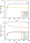 |
Fig. 1 Overall evolution of the instability in time, for the Fid run. Top panel: wave energy evolution. Blue and red lines depict the evolution of transversal perturbations |
![Mathematical equation: $\[\delta B_y^2 / B_0^2\]$](/articles/aa/full_html/2024/08/aa49661-24/aa49661-24-eq36.png)
![Mathematical equation: $\[\delta B_z^2 / B_0^2\]$](/articles/aa/full_html/2024/08/aa49661-24/aa49661-24-eq37.png)
![Mathematical equation: $\[E_x^2 / B_0^2\]$](/articles/aa/full_html/2024/08/aa49661-24/aa49661-24-eq38.png)
3.2.2 Linear phase
We now turn to more quantitative diagnostic of the linear phase of the instability. As expected, the accuracy of our numerical simulations (code and setup) can be tested versus the analytical expectations derived in the previous section. By performing spatial Fourier transform of the time-stacked magnetic field data ![Mathematical equation: $\[F F T\left(B_{y, z}(x, t)\right)=\tilde{B}_{y, z}(k, t)\]$](/articles/aa/full_html/2024/08/aa49661-24/aa49661-24-eq42.png) we can follow the time evolution of intensity in different wave-modes k. We then select the approximate time when the growth is exponential (Δtlin) and then perform the linear fit of
we can follow the time evolution of intensity in different wave-modes k. We then select the approximate time when the growth is exponential (Δtlin) and then perform the linear fit of ![Mathematical equation: $\[\left|\log \left(\tilde{B}_{y, z}\left(k, \Delta t_{\operatorname{lin}}\right)\right)\right|\]$](/articles/aa/full_html/2024/08/aa49661-24/aa49661-24-eq43.png) . This procedure provides the numerical growth rate of different wavemodes, available in the simulation. The smallest wavemode is kmin = 2π/L and the largest is kmax = π/Δ, where Δ is the spatial grid cell size4.
. This procedure provides the numerical growth rate of different wavemodes, available in the simulation. The smallest wavemode is kmin = 2π/L and the largest is kmax = π/Δ, where Δ is the spatial grid cell size4.
The result for three different simulations is presented in Fig. 3. In this figure we show the growth rates derived from simulations (solid blue and red lines), the basic analytical growth rate in the test-particle limit (black dotted line) and the growth rates with no low-frequency approximation (orange and green lines). The blue-coloured line corresponds to the right-handed modes (I+) while the red-coloured lines correspond to the left-handed modes ((I−). Different panels present results from simulations with different beam-to-background number density ratio: ncr/ni = 0.01, 0.005, 0.002 from top to bottom panel, respectively.
We can note that the maximum linear growth rate is obtained at kRL,cr ⋍ 0.7 in agreement with analytical expectations from Equation (13), for all of three simulations. The growth rates are reasonably well reproduced up to kRL,cr ~ 5–6. At higher k some differences appear in the different mode polarisation. Circular right-handed modes always produce higher growth rates than circular left-handed ones. This can be explained by adopting the high-frequency relation derived from Eq. (16). However, it is difficult to provide a firm conclusion because of the increasing effect of numerical noise with k. The agreement with analytical expectations is better for lower ncr/ni, as can be seen by comparing the top panel with the bottom panel. This is expected since analytical calculations have been derived in the quasi-linear limit.
 |
Fig. 2 Wave spectrum I(k) of right-handed and left-handed polarisation waves (top panels: a, d, and g), spatial profile of magnetic field fluctuations δBy,z/B0 (middle panels: b, e, and h) and distribution function of beam electrons and positrons f(Vx) and different times of the simulation (bottom panels: c, f, and i). Left column corresponds to early time (tΩci = 7.6), middle column to the linear phase (tΩci = 76) and right column to the saturated phase of the instability (tΩci = 186). |
3.2.3 Saturated phase
As previously discussed in Sect. 3.2.1 it can be identified that after the linear phase, where the wave growth is exponential, the wave-saturation occurs rapidly (see top panel in Fig. 1). It corresponds to the phase when the wave intensity reaches its maximum and remains nearly constant afterwards. This level defines the saturation of wave intensity as ![Mathematical equation: $\[\delta B_{\text {sat }}^2=\delta B_{y, \text {end }}^2+\delta B_{z \text {.end }}^2\]$](/articles/aa/full_html/2024/08/aa49661-24/aa49661-24-eq44.png) .
.
In Fig. 4, we show the dependence of saturation level of the magnetic field, ![Mathematical equation: $\[\delta B_{\mathrm{sat}}^2 / B_0^2\]$](/articles/aa/full_html/2024/08/aa49661-24/aa49661-24-eq45.png) , on the beam density ncr/ni (panel a) and on the mass ratio mi/me (panel b). The blue circle symbols present the results from different simulations where ncr/ni varies from 0.001 to 0.01; all other parameters being kept the same (mi/me = 100, VD = 0.1c, VA = 0.01c. See Table 2). The dashed black line follows the level derived from the criterion assuming that all of the available momentum lost by the decelerated CR beam (from VD to VA) is transferred to the waves. This criterion was defined in Eq. (17)5. The values measured in the simulations are slightly below the expectation but show very good agreement with the expected trend. We note that such a good agreement is remarkable for a PIC simulation and owing to the simplicity of the analytic criterion6.
, on the beam density ncr/ni (panel a) and on the mass ratio mi/me (panel b). The blue circle symbols present the results from different simulations where ncr/ni varies from 0.001 to 0.01; all other parameters being kept the same (mi/me = 100, VD = 0.1c, VA = 0.01c. See Table 2). The dashed black line follows the level derived from the criterion assuming that all of the available momentum lost by the decelerated CR beam (from VD to VA) is transferred to the waves. This criterion was defined in Eq. (17)5. The values measured in the simulations are slightly below the expectation but show very good agreement with the expected trend. We note that such a good agreement is remarkable for a PIC simulation and owing to the simplicity of the analytic criterion6.
We also derived the saturation in simulations with different mi/me from 50 to 1000 (panel b of Fig. 4). The same criterion provides a good approximation of the saturation level for both ncr/ni = 5 × 10⁻³ and ncr/ni = 10−2 cases. The ‘lack’ of waves is small and can probably be imputed to other channels of dissipation (e.g., background plasma heating, some amount of wave damping).
It is interesting to note that the acquired final velocity of background e−-ion plasma is roughly equal to the saturated wave intensity, ![Mathematical equation: $\[\left\langle V_i\right\rangle_{\mathrm{bg}} / V_{\mathrm{A}} \simeq \delta B_{\mathrm{sat}}^2 / B_0^2\]$](/articles/aa/full_html/2024/08/aa49661-24/aa49661-24-eq46.png) . This was found in all simulations where both quantities could be measured with good confidence. The wave saturation criterion assumes that the momentum lost by CRs when decelerating from VD drift to VA is transferred to waves. Yet, the Alfvén waves are carried by the background fluid that seems to be dragged to the mentioned equality in the process of saturation of the instability.
. This was found in all simulations where both quantities could be measured with good confidence. The wave saturation criterion assumes that the momentum lost by CRs when decelerating from VD drift to VA is transferred to waves. Yet, the Alfvén waves are carried by the background fluid that seems to be dragged to the mentioned equality in the process of saturation of the instability.
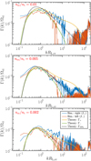 |
Fig. 3 Linear growth rate of the instability Γ as function of the wavenumber k for two polarisation modes: circular right-handed (blue solid line) and left-handed (red solid line). Results for the simulations with three different values of CR density are presented: top panel corresponds to ncr/ni = 0.01, middle panel corresponds to ncr/ni = 5 × 10⁻³, and bottom panel corresponds to ncr/ni = 2 × 10⁻³. In each panel, the solid orange and green lines correspond to the theoretical growth rate using the solution of the full dispersion relation Eq. (16). Black dotted line follows the expectation in test-particle limit from Eq. (13). |
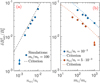 |
Fig. 4 Saturation level of the magnetic fluctuations. Panel a: wave saturation intensity as function of ncr/ni. Blue circles present the results from 1D3V PIC simulations. The red dashed line follows the scaling from Eq. (17) that balances the momentum loss by CRs with momentum gained by waves. The data point at ncr/ni = 10−3 is a lower limit as the simulation ended before a saturated state was reached. Panel b: same but varying mi/me at fixed ncr/ni = 10−2 (blue symbols) and ncr/ni = 5 × 10⁻³ (red symbols). |
3.2.4 Properties of the wave spectrum
Overall intensity is only one aspect of the self-generated waves. The properties of wave spectrum may require more subtle analysis. The wave spectrum after saturation in the Fid simulation, ![Mathematical equation: $\[I_{\text {sat }}(k)=\delta B_{\text {sat }}(k)^2 / B_0^2\]$](/articles/aa/full_html/2024/08/aa49661-24/aa49661-24-eq47.png) , is shown in Fig. 5, top panel. The blue and red solid lines correspond to the final spectrum of right-and left-handed circularly polarised waves, respectively. Previously presented asymmetry between two polarisation modes is observed at kRL,cr > 6. A line-like feature is clearly seen at kRL,cr ~ 170.
, is shown in Fig. 5, top panel. The blue and red solid lines correspond to the final spectrum of right-and left-handed circularly polarised waves, respectively. Previously presented asymmetry between two polarisation modes is observed at kRL,cr > 6. A line-like feature is clearly seen at kRL,cr ~ 170.
In order to understand different cut-off positions for two modes we consider in more detail the proper wavemodes and theoretical growth rates. The corresponding result is presented in Fig. 5, bottom panel. The solutions of the full dispersion relation are obtained by solving Eq. (16). Both real and imaginary (unstable) parts are shown using solid and dashed lines, respectively. The light-wave is shown with a black solid line. Alfvén wave corresponds to low frequency and low-k part of red and blue solid lines. At kRL,cr ≥ 4 – 6 the two branches separate into Whistler (blue solid line) and Ion-cyclotron (red solid line). Alternatively, these two wave branches can be analytically derived with more ease by setting C = 0 (CR term) in the dispersion relation. Solving the equation without the CR term then provides accurate solutions for Whistler and Alfvén/ion-cyclotron (AIC) dispersion relations (e.g., Vainio 2000); which are identical to ℛ-labelled solutions shown in Fig. 5 (bottom panel). By comparing the dashed red/blue lines and solid red/blue lines, one can clearly see that the modes at kRL,cr > 10 are growing into the Whistler (right-handed) and ion-cyclotron (left-handed) wavemodes. This is the first hint to understand the asymmetry between I+ and I−spectra.
We now test the idea that the left-handed polarisation waves (I−) are affected by ion-cyclotron resonance with background plasma. In Fig. 6, we present the saturated spectra of right-handed waves (I+; top panel) and of left-handed waves (I−; bottom panel). Lines of different colours correspond to different mass ratio adopted in the simulations: blue line corresponds to mi/me = 1000 (Fid run), red line corresponds to 400, and orange line corresponds to 100. As can be seen in the top panel, I+ spectrum is only weakly affected by the variation of mi/me, while the I− branch (bottom panel) exhibits a cut that transits to lower kRL,cr with increasing mass ratio. The position of the cut is highlighted using vertical dashed lines. For mi/me = 100 the cut is located at kRL,cr ⋍ 6, while for mi/me = 1000 it is located at kRL,cr ⋍ 1.7.
More systematic analysis of kcut value in large set of simulations is presented in the inset of the bottom panel. Blue circles correspond to values derived from simulations with ncr/ni = 10−2 and red circles are from simulations with ncr/ni = 5 × 10⁻³. All other parameters are the same as in Fid run. The black dashed line follows kcutdi = 0.5 scaling. We observe that all measured values cluster around this scaling. The basic interpretation is that all of I− waves are suppressed for any kRL,cr > 0.5 that falls in the regime where the Alfvén waves transition into Ion-cyclotron branch.
An accurate location of resonant wavenumber can be found by considering the intersection between AIC branch (red solid line in bottom panel of Fig. 5) and ω = Ωci − 3kυth,i (red dotted line in the same panel)7. This gives the cut-off at kcutdi = 0.47, that is basically the same as the result plotted as the dashed line in the inset of Fig. 6. In general, we found that the cut-off wavenumber agrees well with the scaling (Engelbrecht & Strauss 2018; Strauss & le Roux 2019):
![Mathematical equation: $\[k_{\mathrm{cut},-}=\frac{\Omega_{\mathrm{ci}}}{V_{\mathrm{A}}+3 v_{\mathrm{th}, \mathrm{i}}}.\]$](/articles/aa/full_html/2024/08/aa49661-24/aa49661-24-eq48.png) (18)
(18)
Left-handed waves with k > kcut,− are expected to be strongly damped by background plasma. An improved calculation of the damping term following Strauss & le Roux (2019) (Appendix B) shows that the resonance with first two ion-cyclotron harmonics suppresses all left-handed waves at k > kcut,−. Numerical solutions of the dispersion relation accounting for thermal effects in background plasma – using plasma dispersion function – shows as well that kcut,− is an accurate estimate of both the measured values and of full solution of the dispersion relation. To convince ourselves that this is not a numerical effect, we note that the damping of ion-cyclotron waves is a well-observed process in solar wind plasma (Woodham et al. 2018; Bowen et al. 2022, for recent studies). The experimental cut-off scale agrees remarkably well with what we find in the present simulations.
Concerning the I+ spectrum, the value of wavenumber (kcut,+) at which it drops to noise floor level should be regulated by the interaction with the Whistler branch. Using the physical parameters in Fid simulation, we found that the intersection of Whistler branch with ω = Ωce − 3kυth,e occurs at kde ⋍ 0.56. This value is in good agreement with Strauss & le Roux (2019) (see their Fig. 1 and Eqs. (61)–(64)). However, Fid simulation shows that the cut-off of right-handed modes occurs at lower kde ⋍ 0.1 (i.e., kRL,cr ⋍ 10), see top panel of Fig. 5. This value is sensitively lower than expected kcut,+. By inspecting in more detail, we found that there are indeed growing waves up to kde ~ 0.3–0.5 earlier in the simulation. However, the part of spectrum at kde > 0.1 is damped during the saturated phase. Alternatively, in the simulations with lower CR number density (ncr/ni ≤ 5 × 10⁻³) the waves at 0.1 < kde < 0.5 emerge more from the background level and remain at relatively low-intensity level. We have no satisfactory explanation for this different damping effect that increases for larger ncr/ni. Yet, no wave growth is observed for kde > 0.5 in any simulation, that is consistent with expected kcut.+ value.
As a side check, we performed a simulation where the background plasma is composed of pairs (mi = me, run PIC-17 in Table 2). The detailed presentation is reported in Appendix A. To summarise, we found that there is no asymmetry between two polarisation modes of self-excited waves. The initial drift of CRs (beam population) reduced from initial VD = 14.1 VA to exactly VA for both CR electrons and positrons in an identical way. This confirms the idea that the asymmetry is due to the ionic nature of background plasma.
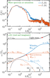 |
Fig. 5 Wave spectrum at saturation and corresponding plasma wave-modes. Top panel: wave spectra in Fid simulation. The blue line for right-handed waves and red line for left-handed waves. Bottom panel: analytic dispersion relation of waves obtained by solving Eq. (16). The real part of ω (solid lines) and instability growth rate for the two polarizations that is the imaginary part of ω (dashed lines). The light-wave is shown with black solid line. The red star symbol at the top left side locates the intersection with ω = 2ωpe line. Alfvén wave corresponds to low frequency and low-k part of red and blue solid lines. At kRL,cr 1 the two branches separate into Whistler (blue solid line) and ion-cyclotron (red solid line). Vertical arrows in bottom panel locate the transition into ion-cyclotron regime (at kdi = 1) for left-handed waves, and electron-cyclotron regime kde = 1 for right-handed waves. The lower red star symbol locates the intersection between the ion-cyclotron branch (red solid line) and Ωce – 3kυth,i (red dotted line). |
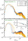 |
Fig. 6 Saturated spectra of right-handed waves (I+; top panel) and of left-handed waves (I−; bottom panel). Lines of different colour correspond to different mass ratio adopted in the simulations: blue line corresponds to mi/me = 1000 (Fid run), red line corresponds to 400, and orange line corresponds to 100. Inset: cut-off wavenumber of left-handed branch for different values of mi/me. Blue circles correspond to values derived from simulations with ncr/ni = 10−2 and red circles are from simulations with ncr/ni = 5 × 10⁻³. The dashed black line follows kcutdi = 0.5. |
3.2.5 Line feature in the wave spectrum
A minor effect of the interaction between CR beam and background plasma produces a high-k line-like feature (e.g., feature at kRL,cr ⋍ 170 in Fig. 2). It was observed in the wave spectra of all simulations except when background plasma is composed of pairs (see Appendix A). As the spectra are only in k space we possess limited information on the frequency of this wave. In order to clarify the nature of this line, we performed dispersion analysis to derive ω(k) from the simulation. This was done by storing the EM fields on the spatial grid at every time-step between tΩci = 95 ant tΩci = 96.6. It corresponds to the end of the linear phase of the instability. By stacking the snapshots of the stored fields and performing 2D FFT on a given field component we derive the dispersion relation ω(k).
In Fig. 7, we present the ω(k) dispersion spectrum performed on Bz component of the magnetic field. The light-wave (EM wave) is well-seen with dispersion ![Mathematical equation: $\[\omega^2 \simeq k^2 c^2+\omega_{\mathrm{pe}}^2\]$](/articles/aa/full_html/2024/08/aa49661-24/aa49661-24-eq50.png) . As the plasma is magnetised, at low-k the EM wave separates into right-and left-handed circular polarisation branches that have slightly different cut-off frequencies. The right-handed mode has the cutoff frequency at ωrh ⋍ ωpe + Ωce/2 while the left-handed branch has the cut-off frequency at ωLH ⋍ ωpe − Ωce/2 (Kulsrud 2005). Exact – textbook – solutions for both branches are over-plotted using black dashed lines. It can be seen that there is a region with enhanced intensity on this branch. This corresponds to a resonance between the EM wave and second harmonic ω = 2ωpe. In terms of the wavenumber, theoretically, it corresponds to
. As the plasma is magnetised, at low-k the EM wave separates into right-and left-handed circular polarisation branches that have slightly different cut-off frequencies. The right-handed mode has the cutoff frequency at ωrh ⋍ ωpe + Ωce/2 while the left-handed branch has the cut-off frequency at ωLH ⋍ ωpe − Ωce/2 (Kulsrud 2005). Exact – textbook – solutions for both branches are over-plotted using black dashed lines. It can be seen that there is a region with enhanced intensity on this branch. This corresponds to a resonance between the EM wave and second harmonic ω = 2ωpe. In terms of the wavenumber, theoretically, it corresponds to ![Mathematical equation: $\[k d_e=\sqrt{3}\]$](/articles/aa/full_html/2024/08/aa49661-24/aa49661-24-eq51.png) . That is in good agreement with the measured position of the instantaneous spectrum I(k), shown in the (b) panel of the figure. This spectrum is the same as presented in Fig. 2 and Fig. 5 but using linear x-axis scale and the wavenumber normalized to
. That is in good agreement with the measured position of the instantaneous spectrum I(k), shown in the (b) panel of the figure. This spectrum is the same as presented in Fig. 2 and Fig. 5 but using linear x-axis scale and the wavenumber normalized to ![Mathematical equation: $\[d_e^{-1}\]$](/articles/aa/full_html/2024/08/aa49661-24/aa49661-24-eq52.png) instead of previously used
instead of previously used ![Mathematical equation: $\[R_{\mathrm{L}, \mathrm{cr}}^{-1}\]$](/articles/aa/full_html/2024/08/aa49661-24/aa49661-24-eq53.png) . In this panel, one can identify the dominant contribution of kde < 0.1 waves and a much less intense region slightly below
. In this panel, one can identify the dominant contribution of kde < 0.1 waves and a much less intense region slightly below ![Mathematical equation: $\[k d_{\mathrm{e}}=\sqrt{3}\]$](/articles/aa/full_html/2024/08/aa49661-24/aa49661-24-eq54.png) . Both panels combined lead to a firm conclusion that this line feature is the second-harmonic emission. We verified in a large set of simulations that the position of this line is always at
. Both panels combined lead to a firm conclusion that this line feature is the second-harmonic emission. We verified in a large set of simulations that the position of this line is always at ![Mathematical equation: $\[k d_{\mathrm{e}} \simeq \sqrt{3}\]$](/articles/aa/full_html/2024/08/aa49661-24/aa49661-24-eq55.png) , independently of n/ni, mi/me, and Tcr values explored.
, independently of n/ni, mi/me, and Tcr values explored.
There is extensive literature on PIC simulations of second-harmonic plasma emission in unmagnetized plasma (e.g., Kasaba et al. 2001; Henri et al. 2019; Krafft & Savoini 2021) and magnetized plasma (e.g., Lee et al. 2022). In the present work, we do not focus on this interaction and limit on basic observation. This is also justified by the fact that this line-emission is largely subdominant to the main instability generated waves in Alfvén branch. It does not seem to have an important effect on the dynamics of the pair beam-driven instability and, more generally, on particle scattering properties.
For completeness, let us describe other noticeable features in Fig. 7. At low ω < Ωce the Whistler branch is clearly seen as well (theoretical dispersion line over plotted with dashed line). The dynamically important part (and by far the brightest spot) of the spectrum corresponds to the region ω/ωpe < 0.1 and kde < 0.1. It is not resolved in this figure as the time window for diagnostics was too small.
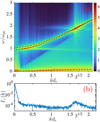 |
Fig. 7 Wave dispersion analysis. Top panel a: wave dispersion ω(k)/ωpe at the final times of the linear phase. From figure simulation (see Table 2 for parameters). The diagnostic was performed on the δBz component between tΩci = 95 ant tΩci = 96.6 (at the end of the linear phase of the instability). Electromagnetic light-wave branch with left and right-handed polarisation is easily identifiable. At low ω < Ωce the Whistler branch is clearly seen as well (theoretical dispersion line over plotted with dashed line). Plasma emission at ω = ωpe is observed and the second harmonic can be observed as well, especially in the brighter zone where it intersects the EM wave. Bottom panel b: I+(k) spectrum at saturation from Fid simulation. It is the same spectrum as in Fig. 5 but plotted using linear x-axis scale and wavenumber plotted in units of |
![Mathematical equation: $\[d_{\mathrm{e}}^{-1}\]$](/articles/aa/full_html/2024/08/aa49661-24/aa49661-24-eq49.png)
4 Discussion
This article addressed the pair-driven instability when the beam propagates through ionic background plasma at super Alfvénic speed. We used fully kinetic particle-in-cell simulations in order to understand the non-linear evolution of the interaction. Combined with detailed analytical derivation in appropriate approximation we verified the accuracy of linear phase of the instability and confirmed some intuitive features, such as a decrease of the beam velocity to near-Alfvénic speed. The intensity of waves at saturation was found to be in good agreement with the momentum transfer criterion: momentum lost by beam particles when they decelerate (erase the anisotropy in the distribution function) is transferred to Alfvén waves. Both Alfvén and kinetic scales were covered by the wavemodes triggered by the instability. This leads to important damping of waves belonging to the ion-cyclotron and Whistler branches. All short-scale waves with kdi ≫ 1 are strongly suppressed by ion-cyclotron resonances with background plasma. We also observed a second harmonic plasma emission. These results might be of interest as input for detailed modelling of particle propagation in TeV halos.
Let us note, however, that by construction our analysis is limited to parallel waves as our simulations were 1D in space. There is no contribution from k⊥ related phenomena. Yet, it is known that at kinetic scales with k⊥di > 1 there is a dominant contribution of kinetic Alfvén waves (KAW), that is well-studied in multidimensional kinetic simulations (e.g., Cerri et al. 2016, 2017). A study of the interplay between self-generated parallel waves by the streaming instability and external turbulence is a topic for future work (recently, a theoretical framework to address this problem was proposed by Cerri 2024).
4.1 Simulations rescaling in comparison with realistic halos
Here, we discuss the relevance of our work to TeV halos, limitations, and possible extensions using other numerical techniques. To start, let us examine how realistic the parameter set chosen in our simulations is. We consider the case of the Geminga pulsar to provide a rough estimate of the ratio ncr/ni in a realistic halo.
The calculation is based on the parameters adopted in Schroer et al. (2023), namely a typical pulsar age of 342 kyrs, a present spin-down luminosity of Lage = 3.26 × 1034 erg/s and an initial spin-down timescale t0 ⋍ 12 kyrs. Under the assumption of pulsar spin down from magnetic dipole radiation (breaking index of 3), the luminosity at time t is
![Mathematical equation: $\[L(t)=L_{\text {age }} \frac{\left(1+t_{\text {age }} / t_0\right)^2}{\left(1+t / t_0\right)^2}.\]$](/articles/aa/full_html/2024/08/aa49661-24/aa49661-24-eq56.png) (19)
(19)
This implies an initial spin-down luminosity L0 = 2.9 × 1037 erg/s at early times t ≪ t0, three orders of magnitude above the present-day value. The particle injection spectrum follows a broken power law8
![Mathematical equation: $\[\begin{aligned}Q(E, t) & =Q_0(t)\left(\frac{E}{E_{\mathrm{b}}}\right)^{-a_{\mathrm{L}}} & & \text { for } \mathrm{E} \leq \mathrm{E}_{\mathrm{b}} \\& =Q_0(t)\left(\frac{E}{E_{\mathrm{b}}}\right)^{-a_{\mathrm{H}}} & & \text { for } \mathrm{E}>\mathrm{E}_{\mathrm{b}},\end{aligned}\]$](/articles/aa/full_html/2024/08/aa49661-24/aa49661-24-eq57.png)
where we use Eb ~ 200 GeV, aL = 1.6, aH = 2.4, in agreement with the ranges of values considered by Schroer et al. (2023). The particle population is energized by the conversion of a constant fraction η ⋍ 1 of the pulsar spin-down power, such that the normalisation Q0 of the injection spectrum is obtained by
![Mathematical equation: $\[\int_{E_{\min }}^{\infty} \mathrm{d} E E Q(E, t)=\eta L(t), \eta \leq 1.\]$](/articles/aa/full_html/2024/08/aa49661-24/aa49661-24-eq58.png) (20)
(20)
The minimum particle energy is taken as Emin = 1 GeV. The average particle energy in the injection spectrum can be approximated as
![Mathematical equation: $\[\begin{aligned}\langle E\rangle & =H\left(a_{\mathrm{L}}, a_{\mathrm{H}}, r\right) \times E_{\mathrm{b}} \\& \simeq \frac{\left(2-a_{\mathrm{L}}\right)^{-1}+\left(a_{\mathrm{H}}-2\right)^{-1}-\left(2-a_{\mathrm{L}}\right)^{-1} r^{2-a_{\mathrm{L}}}}{\left(a_{\mathrm{H}}-1\right)^{-1}-\left(a_{\mathrm{L}}-1\right)^{-1}+\left(a_{\mathrm{L}}-1\right)^{-1} r^{1-a_{\mathrm{L}}}} \times E_{\mathrm{b}},\end{aligned}\]$](/articles/aa/full_html/2024/08/aa49661-24/aa49661-24-eq59.png) (21)
(21)
where r = Emin/Eb. For the adopted parameters, this yields H ⋍ 0.12 hence ⟨E⟩ ⋍ 24 GeV. If Emin = 100 MeV then H ⋍ 0.03 and H goes as r0.6 as r → 0. The factor H is weakly sensitive to aL and aH, for instance keeping Emin = 1 GeV with aL = 1.8 (1.4) and aH = 2.2 (2.6) we find H ⋍ 0.1 (0.17).
We assume that, at each time t, the particle injection rate Q(E, t) is directly released across the surface of the nebula SPWN. The present-day nebula can be approximated as a sphere with radius Rpwn = 0.1 pc (Posselt et al. 2017), but it was likely much larger in the past, when the pulsar was more powerful. The typical size of a bow-shock nebula is the so-called stand-off distance, where pressure in the spherically expanding pulsar wind equals the ram pressure exerted by the ambient medium on the moving pulsar (see Eq. (16) in Gaensler & Slane 2006). This stand-off distance scales as ![Mathematical equation: $\[\sqrt{L} \text { and so } R_{\mathrm{pwn}}(t)=R_{\mathrm{pwn}}\left(t_{\text {age }}\right) \sqrt{L(t) / L_{\text {age }}}\]$](/articles/aa/full_html/2024/08/aa49661-24/aa49661-24-eq60.png) and SPWN ∝ L.
and SPWN ∝ L.
The number density of pairs injected by the nebula at time t can therefore be written as
![Mathematical equation: $\[n_{\mathrm{cr}}(t)=\frac{\eta L(t)}{\langle E\rangle S_{\mathrm{PWN}} V_{\mathrm{D}}}.\]$](/articles/aa/full_html/2024/08/aa49661-24/aa49661-24-eq61.png) (22)
(22)
For a meaningful comparison with the situation implemented in the simulations, we assume that the particles stream across the surface at a velocity VD = 10VA, where VA is the Alfvén speed in the surrounding medium. This numerical choice seems reasonable since VD is basically a free parameter. The typical background gas density around Geminga can be estimated from the absence of Hα emission surrounding the Geminga bow shock to be in the range between ni ~ 10−3 cm−3 (Caraveo et al. 2003) and ni ~ 10−2 cm−3 (Posselt et al. 2017). We use the latter higher bound together with a magnetic field strength of to compute VA = 22 km s−1.
According to Eq. (22), the particle density immediately beyond the surface of the nebula does not depend on time because SPWN ∝ L and all other parameters are considered constant. Using present day values for L = 3.26 × 1034 erg s−1, Rpwn = 0.1 pc and other parameters being specified above (i.e., η = 1, VD = 10VA = 220 km s−1, ⟨E⟩ = 24 GeV), we get ncr ~ 3 × 10⁻⁸ cm−3. Such a value may be considered as a lower limit because the above calculation assumes instantaneous transfer of the pulsar power to the escaping particle flux, whereas there is most likely an accumulation of particles within the nebula for centuries or millennia or more before they can escape or lose their energy. On the other hand, the values of ni and B0 adopted above favour a small Alfvén speed in the surrounding medium, hence a small escape velocity VD and therefore a higher particle density. Overall, the beam-to-background density ratio ncr/ni that can be expected close to the injection zone, that is close to the pulsar wind nebula, is likely in the range 10−6 − 10−5 (with the caveat that the background density at early times might have been higher than 10−2 cm−3). The PIC simulations presented here are therefore not representative of the conditions in the Geminga system.
Another important difference with the astrophysical case resides in our choice of particle distribution. In our simulations, we consider a Maxwell-Jüttner distribution and most of the energy is carried by particles around 10 MeV instead of 200 GeV. Hence, a realistic simulation should have a beam-to-gas density ratio in the range 10−6 − 10−5 and a beam with a bulk energy of Eb ~ 105mec2. It seems that if the resonant streaming instability can be triggered in the environment of evolved pulsars it should be in a region close to the pulsar wind nebula, otherwise the surface term in Eq. (22) produces too much beam dilution. Actually, these values require an unrealistically large numerical box as the PIC method has to resolve the electron skin depth (ideally Debye length). Such high energies would require the use of larger-scale simulations, including a magnetohydrodynamic (MHD) description of the plasma. We therefore discuss briefly in the next subsection an alternative approach based on combining PIC and MHD but leave a more complete study of this regime for future work.
We note that we did not provide a direct extrapolation of the results from our PIC experiments to astrophysical scales for the following reasons: (i) the convergence of simulations with low values of ncr/ni ≤ 10−3 was not reached, (ii) the saturation level of waves confirms intuitive scaling that is already used in the literature in general, and (iii) employing specific non-periodic boundary conditions is needed for direct comparison with a given astrophysical system.
4.2 Large-scale simulations: MHD-PIC
As discussed above, the main limitation is the scale separation that we are able to achieve with full-PIC simulation. This was reflected by the adopted distribution of CRs with an average energy of E ~ 10 MeV. Using MHD-PIC method (Bai et al. 2015; van Marle et al. 2018; Mignone et al. 2018), we can reach higher energies and lower beam densities, which reflect more closely the type of beam-plasma interaction found in astrophysical circumstances. To demonstrate the possibilities of the MHD-PIC method, we performed two simulations in a 2-D box measuring 50 × 0.5 RL, with RL the Larmor radius of the peak of the beam energy distribution. This box is subdivided into a grid of 2000 by 20 grid cells. All boundaries are set to periodic. The box is filled with a stationary thermal plasma and a magnetic field aligned with the x-axis in which the Alfvén speed is set at 0.01 c, the plasma being in equipartition. Through this plasma, we run a beam of non-thermal particles with an advection speed of 0.1 c, and a thermal particle distribution according to a Maxwell–Jüttner prescription with the partial motion being isotropic in the co/moving frame. This beam is made up of an average of 50 particles per particle species per grid cell. We run two MHD-PIC simulations. One with a temperature of Tcr = 10 mec2 and a relative particle density of ncr/ni = 5 × 10⁻³ for comparison with the PIC simulations. The second simulation has a beam temperature of Tcr = 100 mec2 and a relative particle density of ncr/ni = 10−3 to demonstrate MHD-PIC’s ability to reach a more realistic astrophysical parameter space. The simulation is allowed to run while the gas and particles relax.
For the simulation with Tcr = 10 mec2 and = 5 × 10⁻³ (same parameters as full-PIC simulation PIC-3). The result of this comparison is presented in Fig. 8. As can be seen in the upper panel of the figure (magnetic energy evolution), during the linear phase the slope in both PIC and MHD-PIC is very close. Meaning that the fastest growth rates are in good agreement with both techniques. We found that the peak magnetic wave intensity value was lower in MHD-PIC by a factor of ≈ 2 (difference in peak values for blue and red lines). Yet, the wave spectra (bottom panel) were comparing reasonably well, except for the absence of the cut in wave spectra of left-handed modes at kdi > 0.6. This is expected, as the resonant ion-cyclotron absorption effect is absent if the background plasma is treated using an MHD formalism.
For the simulations with a temperature of 100 mec2, the resulting magnetic wave energy evolution in our simulation is shown in Fig. 9. The maximum value ![Mathematical equation: $\[\delta B_{\mathrm{sat}}^2 / B_0^2 \sim 0.05\]$](/articles/aa/full_html/2024/08/aa49661-24/aa49661-24-eq62.png) is reached at tΩci ≈ 400. The level of magnetic fluctuations at the saturation state is consistent with the expected value from Eq. (17) which gives
is reached at tΩci ≈ 400. The level of magnetic fluctuations at the saturation state is consistent with the expected value from Eq. (17) which gives ![Mathematical equation: $\[\delta B_{\mathrm{sat}}^2 / B_0^2 \sim 0.05\]$](/articles/aa/full_html/2024/08/aa49661-24/aa49661-24-eq63.png) for the adopted parameters (we also used me/mi = 100). From Fig. 9, we can also estimate the growth rate of the magnetic field instability for the linear phase, which lasts from tΩci ⋍ 90 until tΩci ⋍ 180. From our simulation, we find a growth rate over that period of approx. Γ/Ωci ~ 3 × 10⁻³ in reasonable agreement with the expected value from Eq. (13).
for the adopted parameters (we also used me/mi = 100). From Fig. 9, we can also estimate the growth rate of the magnetic field instability for the linear phase, which lasts from tΩci ⋍ 90 until tΩci ⋍ 180. From our simulation, we find a growth rate over that period of approx. Γ/Ωci ~ 3 × 10⁻³ in reasonable agreement with the expected value from Eq. (13).
This technique is much less computationally prohibitive than full-PIC simulations and could potentially lead to regimes which are closer to astrophysical parameters. Some improvements such as δf method could be implemented to reach better signal-to-noise ratio and distribution function representation (e.g., Denton & Kotschenreuther 1995; Bai et al. 2019) as well as non-periodic boundary conditions (Bai 2022) that are important to properly describe the saturation of the instability. This work is deferred to a forthcoming study.
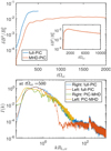 |
Fig. 8 Comparison of the results from full-PIC and MHD-PIC simulations using identical parameters as in run PIC-3 given in Table 2. The top panel presents the average magnetic energy evolution in time for full-PIC (blue solid line) and MHD-PIC (red solid line) techniques. The inset shows the full time-evolution from MHD-PIC simulation, as it runs over a much longer timescale than any full-PIC run. The bottom panel shows the comparison of wave spectra at the time that corresponds to the final time of the full-PIC simulation. Blue and red solid lines show the spectra from full-PIC for right- and left-handed modes, respectively. Green and orange solid lines show the same for MHD-PIC simulation. Note: the spectra from MHD-PIC simulation were upshifted by a factor of ≈ 2 in order to get a better visual comparison. |
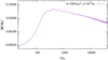 |
Fig. 9 Magnetic energy evolution of a MHD-PIC simulation with Tb = 100mec2 and relative beam density ncr/ni = 10−3. |
5 Conclusion
To conclude, we investigated in detail the evolution of a resonant electron–positron beam-driven streaming instability that develops in a cold background electron-ion plasma. We considered a pair beam following a Maxwell–Jüttner distribution and drifting with respect to the background plasma at a super-Alfvénic speed with initial value VD = 10VA. The simulations were performed using 1D3V Particle-in-Cell simulations.
We find the following main results:
Maximum linear growth rates at scales kRL,cr ~ 0.7 are well recovered. The solutions at smaller scales show polarisation-dependent growth rates, with forward right modes taking over left-handed modes. This effect can be explained by relaxing the condition over the wave frequency in the moving frame to be ≪ Ωci. At high k the right and left-handed modes follow the Whistler/electron-cyclotron and the Alfén/ion-cyclotron branches respectively. The simulations show a reasonable agreement with the analytical solutions. At k ≫ di−1 left-handed modes are damped due to ion-cyclotron resonance and the right-handed modes are cut due to the interaction with the Whistler branch;
We have checked that the criterion for magnetic saturation by momentum transfer from the beam to the waves is well reproduced, with the exception of the low beam density case where the simulations have not converged.
Our results underline the importance of kinetic simulations when subtle effects determine the saturation level and properties of the self-generated spectrum.
We also compared PIC simulations with 1D3V MHD-PIC simulations using the same setup. In particular, we find a reasonable agreement between the two methods. MHD-PIC results show a bit more dissipation, leading to a typical saturated magnetic field energy that is a factor ≈2 below the one obtained using PIC simulations (see Fig. 8).
We finally discuss the rescaling of our numerical setup to the context of gamma-ray halos around evolved pulsars. We find that the kinetic numerical setups have beam-to-background density ratios still several orders of magnitude above the one currently expected in the Geminga pulsar halo. Moreover, the non-thermal particle population carrying the bulk of momentum has typical kinetic energies several orders of magnitude above the range covered by PIC simulations and is unreachable for now. MHD-PIC simulations may partly fill the energy gap to describe the gamma-ray halo more properly. This deserves a future investigation.
Acknowledgements
The authors are grateful to C. Evoli and B. Olmi for fruitful discussions. C. Evoli also provided us with an estimation of the beam-to-background plasma density ratio, which was helpful for the discussion in Sect. 4.1. I.P. is grateful to Silvio Sergio Cerri and Gabriel Fruit for insightful suggestions that improved our understanding of this topic. We acknowledge financial support by ANR for support to the GAMALO project under reference ANR-19-CE31-0014. The simulations have been performed on CALMIP supercomputing resources at Université de Toulouse III (France) under the allocation P20028.
Appendix A Electron-positron background plasma
We want to test whether the asymmetry in the dynamic behaviour of CR positron population with respect to the CR electron population (see Figure 1) and if the spectrum asymmetry is due to the ionic nature of the background plasma. In this appendix, we simplify the simulation setup by considering background plasma being composed of e± pairs (mi = me) instead of ion-electron case studied in the main text. Indeed, such a setup imposes mass and charge symmetry that minimises space charge effects.
Due to typical scales change and the fact that the background mass is no longer dominated by ions we also changed several other parameters as follows: mi = me, ncr/ni = 10−3, Tcr = mec2; Ωce/ωpe = 0.01. The initial drift was unchanged VD/c = 0.1, and background temperature Tbg = 10−3mec2. The deduced Alfvén speed is ![Mathematical equation: $\[V_{\mathrm{A}}=\Omega_{\mathrm{ci}} / \omega_{\mathrm{p}}=\Omega_{\mathrm{ce}} / \omega_{\mathrm{p}}=10^{-2} / \sqrt{2}\]$](/articles/aa/full_html/2024/08/aa49661-24/aa49661-24-eq64.png) , where the division by
, where the division by ![Mathematical equation: $\[\sqrt{2}\]$](/articles/aa/full_html/2024/08/aa49661-24/aa49661-24-eq65.png) is due to mi = me, hence total plasma frequency is
is due to mi = me, hence total plasma frequency is ![Mathematical equation: $\[\omega_p=\sqrt{2} \omega_{\mathrm{pe}}\]$](/articles/aa/full_html/2024/08/aa49661-24/aa49661-24-eq66.png) . These parameters are also reported in Table 2, simulation PIC-17. This setup ensures that the energy density in CRs (kinetic + rest mass) is not dominant compared to the background.
. These parameters are also reported in Table 2, simulation PIC-17. This setup ensures that the energy density in CRs (kinetic + rest mass) is not dominant compared to the background.
In Figure A.1 we present the time evolution of wave energy averaged over the simulation box and drift velocities of four populations (background electrons and positrons, and CR electrons and positrons)9. Despite a high level of noise floor measured in the longitudinal electric field Ex, we can clearly identify the linear phase of the instability between tΩce ⋍ 1000 and tΩce = 1600. The saturation occurs after tΩce = 2500. The intensity of self-generated waves settles at ![Mathematical equation: $\[\delta B_{\mathrm{sat}}^2 / B_0^2 \approx 0.45\]$](/articles/aa/full_html/2024/08/aa49661-24/aa49661-24-eq67.png) . As seen in the bottom panel, the decrease in CR drift is identical for CR electrons and CR positrons. Both drop at the same rate from ~ 14VA to VA, with good accuracy. Concerning the background plasma, it gains some amount of momentum corresponding to final drift ⟨Vbg⟩pos = ⟨Vbg⟩e ⋍ 0.055VA.
. As seen in the bottom panel, the decrease in CR drift is identical for CR electrons and CR positrons. Both drop at the same rate from ~ 14VA to VA, with good accuracy. Concerning the background plasma, it gains some amount of momentum corresponding to final drift ⟨Vbg⟩pos = ⟨Vbg⟩e ⋍ 0.055VA.
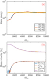 |
Fig. A.1 Same as Figure 1 but for the simulation with electron–positron background mi = me; run PIC-17. Overall time evolution of field intensities (panel a) and drift velocities of different populations (panel b). |
Concerning the wave spectrum and anisotropy in CR distribution function, in Figure A.2 they are presented in the same format as in Figure 2 of the main text. Both branches of wave polarisation are identical at any time of the simulation. Their intensity at three different times is presented with blue and red lines in the top row of the figure. The same is true for the anisotropy in the distribution function (bottom row of the figure). Both CR electrons and positrons undergo a reduction of anisotropy at the same rate. It also reflects in identical behaviour of overall drift velocities. The final state presents a roughly flat f(Vx), such as the anisotropy being basically erased. We also note that the line-like feature in the high-k region of the wave spectrum, observed in simulations with mi ≫ me, is absent here.
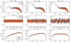 |
Fig. A.2 Wave spectrum I(k) (top panels), magnetic field spatial profile (middle panels) and distribution function of beam electrons and positrons f(Vx) and different times of the simulation. Left column corresponds to early time, middle column to the linear phase and right column to the saturated phase of the instability. |
To complete the analysis of this simulation, we report the derived linear growth rate of the instability in Figure A.3. The agreement between simulation and analytical calculation is good up to kRL,cr ⋍ 10. As in the Fid simulation, we had to use the full dispersion equation that does not assume ω ≪ Ωce. The test-particle limit solution deviates clearly from the measured rate, especially around the fastest-growing wavenumber. We note that waves are not growing at kRL,cr > 10. We recall that the theoretical growth rates were derived in approximation of cold background plasma. But when background thermal effects are considered, the Doppler-shifted cyclotron resonance with thermal electrons and positrons removes waves with kRL,cr > 20 (kRL,cr > 7) if the intersection between ωr and ω = Ωce − kυth,e (ω = Ωce − 3kυth,e) is considered. In Figure A.3 this effect can be seen as an intersection between the black solid line (ωr) and black dot-dashed line (dotted line, respectively). This explains the absence of self-generated waves in kRL,cr > 7 region observed in Figure A.2. At saturation, it seems that the resonance condition with factor of 3, ω = Ωce − 3kυth,e, provides better agreement for the measured cut-off location in the simulation, consistent with what was found in the main text for the cut-off of I−(k), see Sect. 3.2.4.
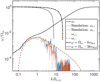 |
Fig. A.3 Real (black solid line) and imaginary part (dashed lines) of the dispersion relation obtained by solving Equation (16), in the case where the background is pair plasma. The growth rates from the corresponding simulation are plotted using blue and red solid lines for right- and left-handed modes), respectively. The fit was not performed on kRL,cr > 50 modes as being strongly affected by thermal noise. The black dot-dashed and dotted lines correspond to Doppler-shifted cyclotron resonance of background thermal plasma: ω = Ωce − kυth,e and ω = Ωce − 3kυth,e, respectively. |
We conclude that the different dynamical behaviour of CR electrons and CR positrons, the asymmetry in the self-generated wave spectrum and line-like emission feature are absent if the background is e± plasma. All these features require the background to be of ionic nature.
Appendix B Linear growth rates: mono-energetic and power-law cases
For completeness, we provide below the growth rates in the quasi-linear limit for power-law and mono-energetic distributions. These two distributions can physically occur in realistic astrophysical systems and could be explored in future numerical simulations. Expressions given below could be useful as analytic expectations for such study.
B.1 Mono-energetic distribution
In the case the beam has a mono-energetic distribution we have ![Mathematical equation: $\[g(p)=p_0^{-2} \delta\left(p-p_0\right)\]$](/articles/aa/full_html/2024/08/aa49661-24/aa49661-24-eq68.png) . It comes
. It comes
![Mathematical equation: $\[\chi_{\mathrm{cr}}=i\left(1-\frac{k V_{\mathrm{D}}}{\omega}\right) \frac{2 \pi^2 e^2}{k \omega} \frac{n_{\mathrm{cr}}}{p_0}.\]$](/articles/aa/full_html/2024/08/aa49661-24/aa49661-24-eq69.png) (B.1)
(B.1)
B.2 Power-law distribution
In the case the beam has a power-law distribution we have for the dimensionless function ![Mathematical equation: $\[g(p)=(\alpha-3) p_0^{-3}\left(p / p_0\right)^{-\alpha}\]$](/articles/aa/full_html/2024/08/aa49661-24/aa49661-24-eq70.png) (Evoli et al. 2018), where p0 ≤ p ≤ pmax. It comes if α > 2:
(Evoli et al. 2018), where p0 ≤ p ≤ pmax. It comes if α > 2:
![Mathematical equation: $\[\chi_{\mathrm{cr}} \simeq i\left(1-\frac{k V_{\mathrm{D}}}{\omega}\right) \frac{2 \pi^2 e^2}{k \omega} \frac{n_{\mathrm{cr}}}{p_0} \frac{(\alpha-3)}{(\alpha-2)}\left(\frac{p_{\min }(k)}{p_0}\right)^{2-\alpha}.\]$](/articles/aa/full_html/2024/08/aa49661-24/aa49661-24-eq71.png) (B.2)
(B.2)
Appendix C Wave decomposition in Fourier space
Here we describe the procedure of construction of the wave intensity in Fourier space, I(k). We follow the same procedure as presented in Bai et al. (2019) (Appendix A), but without assuming that the waves are strictly Alfvénic. The main lines are described below.
The wave intensity I(k) is constructed according to
![Mathematical equation: $\[\int_{k_{\min }}^{k_{\max }} I(k) d k=\left\langle\frac{\delta B^2}{B_0^2}\right\rangle.\]$](/articles/aa/full_html/2024/08/aa49661-24/aa49661-24-eq72.png) (C.1)
(C.1)
The brackets ⟨·⟩ stand for spatial average. A way to decompose circularly polarised modes is to consider the following combination:
![Mathematical equation: $\[C_{ \pm}(x)=\frac{\delta B_y \pm \mathrm{i} \delta B_z}{B_0}.\]$](/articles/aa/full_html/2024/08/aa49661-24/aa49661-24-eq73.png) (C.2)
(C.2)
A discrete Fourier transform of C±(x),
![Mathematical equation: $\[W_{ \pm}\left(k_i\right)=\frac{1}{N} \sum_{n=0}^{N-1} C^{ \pm}\left(x_n\right) e^{-\mathrm{i} k_i x_n} \text {, }\]$](/articles/aa/full_html/2024/08/aa49661-24/aa49661-24-eq74.png) (C.3)
(C.3)
gives the wave amplitude and phase. The wavenumber of mode i is defined as ![Mathematical equation: $\[k_i=\frac{2 \pi}{L_x} i\]$](/articles/aa/full_html/2024/08/aa49661-24/aa49661-24-eq75.png) and Lx = NΔ is the length of the simulation box. The wave intensity is then given by
and Lx = NΔ is the length of the simulation box. The wave intensity is then given by
![Mathematical equation: $\[I_{ \pm}(k)=\left|W_{ \pm}(k)\right|^2 \frac{L_x}{2 \pi}.\]$](/articles/aa/full_html/2024/08/aa49661-24/aa49661-24-eq76.png) (C.4)
(C.4)
With this construction, one defines the dimensionless power in modes of wavenumber k per logarithmic scale as ℱ(k) = kI(k), since dk = 2π/Lx. For clarity, we mainly used I(k) in the figures of the main part of the article.
References
- Abeysekara, A. U., Albert, A., Alfaro, R., et al. 2017a, Science, 358, 911 [NASA ADS] [CrossRef] [Google Scholar]
- Abeysekara, A. U., Albert, A., Alfaro, R., et al. 2017b, ApJ, 843, 40 [Google Scholar]
- Adriani, O., Barbarino, G. C., Bazilevskaya, G. A., et al. 2009, Nature, 458, 607 [CrossRef] [PubMed] [Google Scholar]
- Aguilar, M., Aisa, D., Alvino, A., et al. 2014, Phys. Rev. Lett., 113, 121102 [Google Scholar]
- Aharonian, F., An, Q., Axikegu, Bai, L. X., et al. 2021, Phys. Rev. Lett., 126, 241103 [NASA ADS] [CrossRef] [Google Scholar]
- Amato, E., & Blasi, P. 2009, MNRAS, 392, 1591 [Google Scholar]
- Bai, X.-N. 2022, ApJ, 928, 112 [NASA ADS] [CrossRef] [Google Scholar]
- Bai, X.-N., Caprioli, D., Sironi, L., & Spitkovsky, A. 2015, ApJ, 809, 55 [NASA ADS] [CrossRef] [Google Scholar]
- Bai, X.-N., Ostriker, E. C., Plotnikov, I., & Stone, J. M. 2019, ApJ, 876, 60 [NASA ADS] [CrossRef] [Google Scholar]
- Bao, L.-Z., Fang, K., Bi, X.-J., & Wang, S.-H. 2022, ApJ, 936, 183 [NASA ADS] [CrossRef] [Google Scholar]
- Bowen, T. A., Chandran, B. D. G., Squire, J., et al. 2022, Phys. Rev. Lett., 129, 165101 [NASA ADS] [CrossRef] [Google Scholar]
- Caraveo, P. A., Bignami, G. F., De Luca, A., et al. 2003, Science, 301, 1345 [CrossRef] [Google Scholar]
- Cerri, S. S. 2024, A&A, in press, https://doi.org/10.1051/0004-6361/202449492 [NASA ADS] [CrossRef] [EDP Sciences] [Google Scholar]
- Cerri, S. S., Califano, F., Jenko, F., Told, D., & Rincon, F. 2016, ApJ, 822, L12 [NASA ADS] [CrossRef] [Google Scholar]
- Cerri, S. S., Servidio, S., & Califano, F. 2017, ApJ, 846, L18 [NASA ADS] [CrossRef] [Google Scholar]
- De La Torre Luque, P., Fornieri, O., & Linden, T. 2022, Phys. Rev. D, 106, 123033 [CrossRef] [Google Scholar]
- Denton, R. E., & Kotschenreuther, M. 1995, J. Computat. Phys., 119, 283 [NASA ADS] [CrossRef] [Google Scholar]
- Derouillat, J., Beck, A., Pérez, F., et al. 2018, Comput. Phys. Commun., 222, 351 [NASA ADS] [CrossRef] [Google Scholar]
- Dieckmann, M. E., Alejo, A., & Sarri, G. 2018, Phys. Plasmas, 25, 062122 [NASA ADS] [CrossRef] [Google Scholar]
- Dieckmann, M. E., Folini, D., Hotz, I., et al. 2019, A&A, 621, A142 [NASA ADS] [CrossRef] [EDP Sciences] [Google Scholar]
- Dieckmann, M. E., Folini, D., Walder, R., Charlet, A., & Marcowith, A. 2022, Phys. Plasmas, 29, 092103 [NASA ADS] [CrossRef] [Google Scholar]
- Di Mauro, M., Manconi, S., & Donato, F. 2019, Phys. Rev. D, 100, 123015 [NASA ADS] [CrossRef] [Google Scholar]
- Di Mauro, M., Manconi, S., Negro, M., & Donato, F. 2021, Phys. Rev. D, 104, 103002 [NASA ADS] [CrossRef] [Google Scholar]
- Engelbrecht, N. E., & Strauss, R. D. T. 2018, ApJ, 856, 159 [Google Scholar]
- Evoli, C., Linden, T., & Morlino, G. 2018, Phys. Rev. D, 98, 063017 [NASA ADS] [CrossRef] [Google Scholar]
- Evoli, C., Amato, E., Blasi, P., & Aloisio, R. 2021, Phys. Rev. D, 103, 083010 [NASA ADS] [CrossRef] [Google Scholar]
- Fang, K., Bi, X.-J., Yin, P.-F., & Yuan, Q. 2018, ApJ, 863, 30 [CrossRef] [Google Scholar]
- Fang, K., Bi, X.-J., & Yin, P.-F. 2019, MNRAS, 488, 4074 [NASA ADS] [CrossRef] [Google Scholar]
- Foote, E. A., & Kulsrud, R. M. 1979, ApJ, 233, 302 [NASA ADS] [CrossRef] [Google Scholar]
- Gaensler, B. M., & Slane, P. O. 2006, ARA&A, 44, 17 [Google Scholar]
- Gupta, S., Caprioli, D., & Haggerty, C. C. 2021, ApJ, 923, 208 [NASA ADS] [CrossRef] [Google Scholar]
- Haverkorn, M., Brown, J. C., Gaensler, B. M., & McClure-Griffiths, N. M. 2008, ApJ, 680, 362 [Google Scholar]
- Henri, P., Sgattoni, A., Briand, C., Amiranoff, F., & Riconda, C. 2019, J. Geophys. Res. (Space Phys.), 124, 1475 [NASA ADS] [CrossRef] [Google Scholar]
- H.E.S.S. Collaboration (Aharonian, F., et al.) 2023, A&A, 673, A148 [NASA ADS] [CrossRef] [EDP Sciences] [Google Scholar]
- Holcomb, C., & Spitkovsky, A. 2019, ApJ, 882, 3 [NASA ADS] [CrossRef] [Google Scholar]
- Jóhannesson, G., Porter, T. A., & Moskalenko, I. V. 2019, ApJ, 879, 91 [CrossRef] [Google Scholar]
- Kasaba, Y., Matsumoto, H., & Omura, Y. 2001, J. Geophys. Res., 106, 18693 [NASA ADS] [CrossRef] [Google Scholar]
- Krafft, C., & Savoini, P. 2021, ApJ, 917, L23 [NASA ADS] [CrossRef] [Google Scholar]
- Kulsrud, R. M. 2005, Plasma Physics for Astrophysics (Princeton University Press) [Google Scholar]
- Lee, S.-Y., Yoon, P. H., Lee, E., & Tu, W. 2022, ApJ, 924, 36 [NASA ADS] [CrossRef] [Google Scholar]
- López-Coto, R., & Giacinti, G. 2018, MNRAS, 479, 4526 [CrossRef] [Google Scholar]
- Manconi, S., Di Mauro, M., & Donato, F. 2020, Phys. Rev. D, 102, 023015 [NASA ADS] [CrossRef] [Google Scholar]
- Marcowith, A., van Marle, A. J., & Plotnikov, I. 2021, Phys. Plasmas, 28, 080601 [NASA ADS] [CrossRef] [Google Scholar]
- Marret, A., Ciardi, A., Smets, R., & Fuchs, J. 2021, MNRAS, 500, 2302 [Google Scholar]
- Martin, P., Marcowith, A., & Tibaldo, L. 2022a, A&A, 665, A132 [NASA ADS] [CrossRef] [EDP Sciences] [Google Scholar]
- Martin, P., Tibaldo, L., Marcowith, A., & Abdollahi, S. 2022b, A&A, 666, A7 [NASA ADS] [CrossRef] [EDP Sciences] [Google Scholar]
- Mignone, A., Bodo, G., Vaidya, B., & Mattia, G. 2018, ApJ, 859, 13 [CrossRef] [Google Scholar]
- Mukhopadhyay, P., & Linden, T. 2022, Phys. Rev. D, 105, 123008 [NASA ADS] [CrossRef] [Google Scholar]
- Plotnikov, I., Ostriker, E. C., & Bai, X.-N. 2021, ApJ, 914, 3 [CrossRef] [Google Scholar]
- Posselt, B., Pavlov, G. G., Slane, P. O., et al. 2017, ApJ, 835, 66 [CrossRef] [Google Scholar]
- Profumo, S., Reynoso-Cordova, J., Kaaz, N., & Silverman, M. 2018, Phys. Rev. D, 97, 123008 [NASA ADS] [CrossRef] [Google Scholar]
- Recchia, S., Di Mauro, M., Aharonian, F. A., et al. 2021, Phys. Rev. D, 104, 123017 [NASA ADS] [CrossRef] [Google Scholar]
- Schroer, B., Evoli, C., & Blasi, P. 2023, Phys. Rev. D, 107, 123020 [CrossRef] [Google Scholar]
- Strauss, R. D., & le Roux, J. A. 2019, ApJ, 872, 125 [NASA ADS] [CrossRef] [Google Scholar]
- Tang, X., & Piran, T. 2019, MNRAS, 484, 3491 [CrossRef] [Google Scholar]
- Torres, D. F., Cillis, A., Martín, J., & de Oña Wilhelmi, E. 2014, J. High Energy Astrophys., 1, 31 [NASA ADS] [Google Scholar]
- Vainio, R. 2000, ApJS, 131, 519 [NASA ADS] [CrossRef] [Google Scholar]
- van Marle, A. J., Casse, F., & Marcowith, A. 2018, MNRAS, 473, 3394 [NASA ADS] [CrossRef] [Google Scholar]
- Woodham, L. D., Wicks, R. T., Verscharen, D., & Owen, C. J. 2018, ApJ, 856, 49 [CrossRef] [Google Scholar]
- Zweibel, E. G., & Everett, J. E. 2010, ApJ, 709, 1412 [NASA ADS] [CrossRef] [Google Scholar]
Pre-existing turbulence could help because it may provide a supplementary source of particle scattering if acting on an appropriate scale. Yet, this effect has to be assessed with a dedicated study.
In this work, we use the test-particle terminology following Evoli et al. (2018). It is valid as long as the electron–positron beam is not modifying the dispersion relation of Alfvén waves, that is when the amplitude of excited waves is small: δB ≪ B0. When this limit is not satisfied, the instability drives either strongly modified Alfvén waves or waves or different nature and scale (e.g., kinetic Alfvén waves, Whistler, ion-cyclotron, etc.).
In this case, the charge and current of one macro-particle is distributed over 5 spatial grid-points (Derouillat et al. 2018).
Waves at k > π/Δ are not resolved, as the Nyquist wavenumber is 2π/Δ.
We used the fact that for an ultra-relativistic Maxwell–Jüttner distribution (see Eq. (9)) with θ = kBTcr/mec2 ≫ 1 the average particle momentum is ⟨p⟩ = 3kBTcr/c
The exception is the simulation with the lowest ncr/ni = 10−3. Here, the simulation was too short to reach saturation. We directly verified that the linear phase was still ongoing at the final time of the run.
We found that the factor 3υth,i in this relation provides better agreement with simulation, instead of more standard υth,i. It was argued in Engelbrecht & Strauss (2018) that this factor captures better the range of resonantly interacting background particles.
The injection spectrum is also expected to feature a time-varying cutoff at an energy Ec, for instance to reflect the progressive decrease of the maximum potential drop, which would lead to ![Mathematical equation: $\[E_{\mathrm{c}}(t)=1.7 \sqrt{L(t) / 10^{36} \mathrm{erg} \mathrm{s}^{-1}} ~\mathrm{PeV}\]$](/articles/aa/full_html/2024/08/aa49661-24/aa49661-24-eq77.png) . We neglect this here because the high typical values for this cutoff energy have no impact on our particle density estimates.
. We neglect this here because the high typical values for this cutoff energy have no impact on our particle density estimates.
This figure is basically the same as Figure 1 but for the e± background simulation.
All Tables
All Figures
|
Fig. 1 Overall evolution of the instability in time, for the Fid run. Top panel: wave energy evolution. Blue and red lines depict the evolution of transversal perturbations |
| In the text | |
|
Fig. 2 Wave spectrum I(k) of right-handed and left-handed polarisation waves (top panels: a, d, and g), spatial profile of magnetic field fluctuations δBy,z/B0 (middle panels: b, e, and h) and distribution function of beam electrons and positrons f(Vx) and different times of the simulation (bottom panels: c, f, and i). Left column corresponds to early time (tΩci = 7.6), middle column to the linear phase (tΩci = 76) and right column to the saturated phase of the instability (tΩci = 186). |
| In the text | |
|
Fig. 3 Linear growth rate of the instability Γ as function of the wavenumber k for two polarisation modes: circular right-handed (blue solid line) and left-handed (red solid line). Results for the simulations with three different values of CR density are presented: top panel corresponds to ncr/ni = 0.01, middle panel corresponds to ncr/ni = 5 × 10⁻³, and bottom panel corresponds to ncr/ni = 2 × 10⁻³. In each panel, the solid orange and green lines correspond to the theoretical growth rate using the solution of the full dispersion relation Eq. (16). Black dotted line follows the expectation in test-particle limit from Eq. (13). |
| In the text | |
|
Fig. 4 Saturation level of the magnetic fluctuations. Panel a: wave saturation intensity as function of ncr/ni. Blue circles present the results from 1D3V PIC simulations. The red dashed line follows the scaling from Eq. (17) that balances the momentum loss by CRs with momentum gained by waves. The data point at ncr/ni = 10−3 is a lower limit as the simulation ended before a saturated state was reached. Panel b: same but varying mi/me at fixed ncr/ni = 10−2 (blue symbols) and ncr/ni = 5 × 10⁻³ (red symbols). |
| In the text | |
|
Fig. 5 Wave spectrum at saturation and corresponding plasma wave-modes. Top panel: wave spectra in Fid simulation. The blue line for right-handed waves and red line for left-handed waves. Bottom panel: analytic dispersion relation of waves obtained by solving Eq. (16). The real part of ω (solid lines) and instability growth rate for the two polarizations that is the imaginary part of ω (dashed lines). The light-wave is shown with black solid line. The red star symbol at the top left side locates the intersection with ω = 2ωpe line. Alfvén wave corresponds to low frequency and low-k part of red and blue solid lines. At kRL,cr 1 the two branches separate into Whistler (blue solid line) and ion-cyclotron (red solid line). Vertical arrows in bottom panel locate the transition into ion-cyclotron regime (at kdi = 1) for left-handed waves, and electron-cyclotron regime kde = 1 for right-handed waves. The lower red star symbol locates the intersection between the ion-cyclotron branch (red solid line) and Ωce – 3kυth,i (red dotted line). |
| In the text | |
|
Fig. 6 Saturated spectra of right-handed waves (I+; top panel) and of left-handed waves (I−; bottom panel). Lines of different colour correspond to different mass ratio adopted in the simulations: blue line corresponds to mi/me = 1000 (Fid run), red line corresponds to 400, and orange line corresponds to 100. Inset: cut-off wavenumber of left-handed branch for different values of mi/me. Blue circles correspond to values derived from simulations with ncr/ni = 10−2 and red circles are from simulations with ncr/ni = 5 × 10⁻³. The dashed black line follows kcutdi = 0.5. |
| In the text | |
|
Fig. 7 Wave dispersion analysis. Top panel a: wave dispersion ω(k)/ωpe at the final times of the linear phase. From figure simulation (see Table 2 for parameters). The diagnostic was performed on the δBz component between tΩci = 95 ant tΩci = 96.6 (at the end of the linear phase of the instability). Electromagnetic light-wave branch with left and right-handed polarisation is easily identifiable. At low ω < Ωce the Whistler branch is clearly seen as well (theoretical dispersion line over plotted with dashed line). Plasma emission at ω = ωpe is observed and the second harmonic can be observed as well, especially in the brighter zone where it intersects the EM wave. Bottom panel b: I+(k) spectrum at saturation from Fid simulation. It is the same spectrum as in Fig. 5 but plotted using linear x-axis scale and wavenumber plotted in units of |
| In the text | |
|
Fig. 8 Comparison of the results from full-PIC and MHD-PIC simulations using identical parameters as in run PIC-3 given in Table 2. The top panel presents the average magnetic energy evolution in time for full-PIC (blue solid line) and MHD-PIC (red solid line) techniques. The inset shows the full time-evolution from MHD-PIC simulation, as it runs over a much longer timescale than any full-PIC run. The bottom panel shows the comparison of wave spectra at the time that corresponds to the final time of the full-PIC simulation. Blue and red solid lines show the spectra from full-PIC for right- and left-handed modes, respectively. Green and orange solid lines show the same for MHD-PIC simulation. Note: the spectra from MHD-PIC simulation were upshifted by a factor of ≈ 2 in order to get a better visual comparison. |
| In the text | |
|
Fig. 9 Magnetic energy evolution of a MHD-PIC simulation with Tb = 100mec2 and relative beam density ncr/ni = 10−3. |
| In the text | |
|
Fig. A.1 Same as Figure 1 but for the simulation with electron–positron background mi = me; run PIC-17. Overall time evolution of field intensities (panel a) and drift velocities of different populations (panel b). |
| In the text | |
|
Fig. A.2 Wave spectrum I(k) (top panels), magnetic field spatial profile (middle panels) and distribution function of beam electrons and positrons f(Vx) and different times of the simulation. Left column corresponds to early time, middle column to the linear phase and right column to the saturated phase of the instability. |
| In the text | |
|
Fig. A.3 Real (black solid line) and imaginary part (dashed lines) of the dispersion relation obtained by solving Equation (16), in the case where the background is pair plasma. The growth rates from the corresponding simulation are plotted using blue and red solid lines for right- and left-handed modes), respectively. The fit was not performed on kRL,cr > 50 modes as being strongly affected by thermal noise. The black dot-dashed and dotted lines correspond to Doppler-shifted cyclotron resonance of background thermal plasma: ω = Ωce − kυth,e and ω = Ωce − 3kυth,e, respectively. |
| In the text | |
Current usage metrics show cumulative count of Article Views (full-text article views including HTML views, PDF and ePub downloads, according to the available data) and Abstracts Views on Vision4Press platform.
Data correspond to usage on the plateform after 2015. The current usage metrics is available 48-96 hours after online publication and is updated daily on week days.
Initial download of the metrics may take a while.