| Issue |
A&A
Volume 688, August 2024
|
|
|---|---|---|
| Article Number | A76 | |
| Number of page(s) | 13 | |
| Section | Extragalactic astronomy | |
| DOI | https://doi.org/10.1051/0004-6361/202449422 | |
| Published online | 05 August 2024 | |
Resolving high-z galaxy cluster properties through joint X-ray and millimeter analysis: Case study of SPT-CLJ0615-5746
1
Dipartimento di Fisica, Università di Roma ‘Tor Vergata’, Via della Ricerca Scientifica 1, 00133 Roma, Italy
2
INFN, Sezione di Roma ‘Tor Vergata’, Via della Ricerca Scientifica, 1, 00133 Roma, Italy
e-mail: This email address is being protected from spambots. You need JavaScript enabled to view it.
3
INFN-Padova, Via Marzolo 8, 35131 Padova, Italy
Received:
30
January
2024
Accepted:
15
April
2024
Abstract
We present a joint millimetric and X-ray analysis of hot gas properties in the distant galaxy cluster SPT-CLJ0615-5746 (z = 0.972). Combining Chandra observations with the South Pole Telescope (SPT) and Planck data, we performed radial measurements of thermodynamical quantities up to a characteristic radius of 1.2 R500. We exploited the high angular resolution of Chandra and SPT to map the innermost region of the cluster and the high sensitivity to the larger angular scales of Planck to constrain the outskirts and improve the estimation of the cosmic microwave background and the galactic thermal dust emissions. In addition to maximizing the accuracy of radial temperature measurements, our joint analysis allows us to test the consistency between X-ray and millimetric derivations of thermodynamic quantities via the introduction of a normalization parameter (ηT) between X-ray and millimetric temperature profiles. This approach reveals a substantial high value of the normalization parameter, ηT = 1.45−0.18+0.17, suggesting that the gas halo is aspherical. Assuming hot gas hydrostatic equilibrium within complementary angular sectors that intercept the major and minor elongation of the X-ray image, we infer a halo mass profile that results from an effective compensation of azimuthal variations of gas densities by variations in the ηT parameter. Consistent with earlier integrated X-ray and millimetric measurements, we infer a cluster mass of M500HE = 10.67−0.50+0.62 1014 M⊙.
Key words: techniques: image processing / galaxies: clusters: general / galaxies: clusters: intracluster medium / galaxies: clusters: individual: SPT-CLJ0615–5746 / cosmic background radiation / cosmology: observations
© The Authors 2024
 Open Access article, published by EDP Sciences, under the terms of the Creative Commons Attribution License (https://creativecommons.org/licenses/by/4.0), which permits unrestricted use, distribution, and reproduction in any medium, provided the original work is properly cited.
This article is published in open access under the Subscribe to Open model. This email address is being protected from spambots. You need JavaScript enabled to view it. to support open access publication.
1. Introduction
Being the most massive gravitationally bound structures, galaxy clusters most likely formed recently via the collapse of matter haloes and the accretion of substructures in their periphery. As closed pieces of the Universe, Galaxy clusters are laboratories that can reveal the nature of the matter content of the Universe, including dark matter and baryons, and the interplay between these components during the late time of cosmic evolution.
Baryons in galaxy clusters prevalently take the form of a hot ionized atmosphere, detectable at the same time as a result of its inverse-Compton scattering of CMB photons (called the SZ effect; Sunyaev & Zeldovich 1972) and in the X-ray band via its bremsstrahlung emission. Due to the redshift independence of the SZ effect, millmetric surveys recently allowed us to sample the cluster population over a significant fraction of its evolution with cosmic times. In particular, the all-sky Planck catalog of SZ sources (Planck Collaboration XXVII 2016) contains 1203 confirmed clusters with a mean mass of 4.82 × 10¹⁴ M⊙ over a redshift range between 0.011 and 0.972. Instead, the first South Pole Telescope (SPT) receiver was employed to carry out the 2500 square degree SPT-SZ survey (Bleem et al. 2015). The catalog features 677 cluster candidates, of which 516 have optical and/or infrared counterparts. The median mass of the catalog is  with a median redshift of z = 0.55, while the highest-redshift systems reach z > 1.4. The second receiver was used to conduct the 500 square degree SPTpol survey (Bleem et al. 2024), yielding a new catalog containing 689 detections. Out of these, 544 are confirmed clusters with identified counterparts in optical and infrared data. The confirmed sample has a median mass of
  and a median redshift of z = 0.7. The highest-redshift clusters extend up to z ∼ 1.6, with 21% of the samples at z > 1. X-ray observations will ideally complement millimetric observations to help in understanding the hot gas thermodynamics in these newly detected clusters. This is particularly significant since the SZ effect and thermal bremsstrahlung radiation are predominantly sensitive to the hot gas pressure and density, respectively, and thus a combination of the two measurements would allow a direct estimation of the hydrostatic mass and the other thermodynamic profiles (Ruppin et al. 2021; Adam et al. 2024). However, cross-calibration issues of the instruments, the morphology of the systems, or the cosmological model can cause discrepancies between the two independent observations of the hot gas. Such systematics can be accounted for through the introduction of a normalization parameter, ηT, between X-ray and millimetric temperature profiles, enabling the effective combination of the two data sets. In the ideal scenario we would expect ηT = 1, but in more realistic cases ηT is expected to deviate from one due to the various factors mentioned earlier (Bourdin et al. 2017; Ghirardini et al. 2019; Kozmanyan et al. 2019).
To investigate the ICM thermodynamics in high-redshift clusters, we present a joint millimeter and X-ray analysis of hot gas properties of SPT-CLJ0615-4756, the most distant galaxy cluster in the Planck catalog of SZ sources (Planck name: PSZ2 G266.54-27.31). This cluster is also included in the SPT-SZ cluster catalog with a mass estimates of  , making it one of the most massive clusters in the survey. Studies of this cluster have been conducted at various wavelengths. Optical research (Schrabback et al. 2018; Connor et al. 2019) and X-ray analysis (Bartalucci et al. 2017, 2018) both revealed an elongated shape and a high core-excised X-ray temperature. These results are in agreement with the large ηT value reported by Bourdin et al. (2017) (ηT ∼ 1.7), which suggests a high level of asphericity. Recently, Jiménez-Teja et al. (2023) used the intracluster light (ICL) fraction as an indicator of the dynamical stage of the cluster and found that the ICL fraction distribution of SPT-CLJ0615-4756 is more indicative of an active system than a relaxed cluster.
In this work we present an updated version of the pipeline developed in Bourdin et al. (2017) and Oppizzi et al. (2023) to analyze the properties of such a high-redshift cluster. We took advantage of the multiwavelength data from Chandra X-ray Observatory, Planck, and the South Pole Telescope (SPT) to uncover the structure of the ICM out to distances beyond R500.
We present the three data sets in Sect. 2 and their processing in Sect. 3. We discuss our fitting methods in Sect. 4, with the parametric modeling and analysis of the ICM properties in Sect. 5. Our summary and conclusions are presented in Sect. 6. In this paper we assume a flat ΛCDM cosmology with Ωm = 0.3, ΩΛ = 0.7, and H0 = 70 km s−1 Mpc−1. We define R500 and M500 in terms of the critical density ρc(z) at cluster redshift z as  .
.
2. Data sets
SPT-CLJ0615-5746 (Planck name: PLCKG266.6-27.3) is the highest-redshift cluster detected by Planck via SZ effects (Planck Collaboration XXVII 2016). This system also belongs to the SPT-SZ cluster sample (Bleem et al. 2015) and has additionally been observed with Chandra with an exposure time of ∼240ks (proposal 13800663, PI P. Mazzotta). The latter observations were performed using the Advanced CCD imaging spectrometer (ACIS, Garmire et al. 2003) and are part of the public data available in the Chandra data archive1.
The Planck data come from the second public data release2 (PR2) of Planck High-Frequency Instrument (HFI). The data set consists of six full-sky maps in HEALPIX format with an Nside value of 2048, meaning a pixel angular size of 1.72 arcmin. These maps were obtained from the full 30-month mission and had nominal frequencies of 100, 143, 217, 353, 545, and 857 GHz, with resolution 9.66, 7.22, 4.90, 4.92, 4.67, and 4.22 arcmin full width at half maximum (FWHM) Gaussian, respectively.
In addition, we used the public SPT data3 from the 2500 square degree SPT–SZ survey from 20h to 7h in right ascension and from −65° to −40° in declination, which consists of three maps with frequency bands centered at 95, 150, and 220 GHz with 1.7, 1.2, and 1.0 arcmin resolution, respectively. These public data are convolved with a common Gaussian beam with 1.75 arcmin FWHM and released in the HEALPIX format with resolution parameter Nside = 8192 corresponding to a pixel angular size of 0.43 arcmin. The main properties of the cluster and our X-ray data set information are listed in Table 1.
Main properties of SPT-CLJ0615-5746.
3. Data processing
3.1. Chandra observations
We analyze the X-ray data following the scheme used in Bourdin et al. (2017). The CDFS from the Chandra Data Archive are first pre-processed to generate calibrated event files for the data reduction with the CIAO tools, version 4.13 and calibration files version 4.9.6. To prevent any contamination from flares or high-background periods, we followed Bourdin & Mazzotta (2008), Bourdin et al. (2013) and removed all the events that deviate more than 3σ from the light curve profile. We identified and mask all point sources that can contaminate our signals using SExtractor (Bertin & Arnouts 1996).
The X-ray background of the Chandra telescope is characterized by instrumental (particle background) and astrophysical components. To mitigate potential systematic errors arising from residual spatial fluctuations of the particle background model across the entire Field of View, we fitted the normalization of the particle background model in a sky region that surrounds the cluster itself. This involves considering all pixels between  and
and  from the X-ray peak, using the [9.5 − 10.6],keV band. To ensure that contamination from the cluster is not considered, we extracted the spectrum within the specified radial range, calculating a signal-to-noise ratio (S/N) of approximately 4% in our energy band. This low S/N is expected, as at these energies, the ACIS-I effective area decreases by a factor of approximately 100, resulting in cluster counts comparable to the level of systematic in the background estimation. This approach allowed us to accurately estimate the background surrounding the observed cluster while simultaneously minimizing the potential risk of contamination from the cluster itself. The astrophysical component originates from the foreground emission of our Galaxy and the cosmic X-ray background (CXB) as a result of the unresolved point sources. To have high photon statistics, we fitted the normalization of these components considering all the pixels that lie more than
  from the X-ray peak following the spectral and spatial features described in Bourdin et al. (2013): the CXB is modeled with an absorbed power law of index γ = 1.42, while the emission associated with our Galaxy can be modeled by the sum of two absorbed thermal components accounting for the Galactic transabsorption emission (kT1 = 0.099 keV and kT2 = 0.248 keV).
Figure 1 shows the zoomed wavelet map after the cleaning procedure. The image is produced using a denoising algorithm based on a wavelet reconstruction of the maps (Starck et al. 2009; Bourdin et al. 2013). The map is background subtracted and covers a region of  with the X-ray surface brightness extracted in the soft X-ray band (0.5, 2.5 keV). The black cross represents the X-ray peak, identified as the coordinates of the maximum of a sparse wavelet-denoised (Starck et al. 2002, 2009) surface brightness map. We consider this position as the cluster center to compute all the radial profiles for both X-ray and SZ analysis.
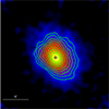 |
Fig. 1. Wavelet-denoised image of the Chandra X-ray emission of SPT-CLJ0615-5746. The map shows the backgroud-subtracted surface brightness computed in the energy range [0.5, 2.5] keV. It covers an area of |


3.2. Millimetric observations
To analyze the millimetric data and extract the pressure profile of the cluster SPT-CLJ0615-5746, we used an updated version of the pipeline described in Oppizzi et al. (2023). This new pipeline essentially consists of two steps using both SPT and Planck maps: a component separation to remove the background (CMB background) and the foreground (Galactic contaminants) in the SPT and Planck observations separately and then a combination of the two data sets to derive the pressure profile.
3.2.1. Planck observations
The galaxy cluster signal was extracted using Planck HFI data from the full 30-months mission. The all-sky HFI frequency maps are re-projected on smaller tiles of 512 × 512 pixels into the tangential plane, with a resolution of 1 arcmin/pixel (corresponding to ∼8.5° ×8.5°) around the cluster X-ray peak. As a first consideration, we removed all point sources from the HFI maps, masking all the ones detected in the PCCS2 and PCCS2E catalogs (Planck Collaboration XXVI 2016). These maps incorporate the SZ and dust cluster signal combined with Galactic foreground and CMB anisotropies. Additionally, other contributions come from cosmic infrared and SZ backgrounds, along with instrumental offsets. To isolate the millimetric cluster signal from the other components, we use the technique developed in Bourdin et al. (2017). Here we summarize the pipeline:
-
We reduced the angular resolution of HFI maps in the range 217 − 857 GHz, to a common value of 5 arcmin and then, to remove the large scale fluctuations, we convolved each frequency map with a third-order B-spline kernel (Curry & Schoenberg 1965). This procedure yields a smoothed image that we subtracted from the raw image to get the maps filtered from large-scale anisotropies.
-
To create a spatial template for the Galactic thermal dust anisotropies (GTD), we denoised the 857 GHz map using an isotropic undecimated wavelet transform (Starck et al. 2007) and applying a thresholding (3σ) on the coefficients. Then we modeled the SED of these anisotropies as a two temperature (Tcold and Thot) gray body (Meisner & Finkbeiner 2014). Defining βd,cold and βd,hot as spectral indexes, fcold as the cold component fraction and q1 and q2 the ratios of far-infrared emission to optical absorption, the SED, is as follows:
![Mathematical equation: $$ \begin{aligned} s_{\rm GTD}(\nu )&=\Bigg [\frac{q_1f_{\text{ cold}}}{q_2}\Bigg (\frac{\nu }{\nu _0}\Bigg )^{\beta _{\text{ d,cold}}}B_{\nu }(T_{\text{ cold}}) \nonumber \\&\quad +(1-f_{\text{ cold}})\Bigg (\frac{\nu }{\nu _0}\Bigg )^{\beta _{\text{ d,hot}}}B_{\nu }(T_{\text{ hot}})\Bigg ]\,. \end{aligned} $$](/articles/aa/full_html/2024/08/aa49422-24/aa49422-24-eq21.gif) (1)
(1)Here Bν is the Planck function and we left free the overall amplitude, fcold and βd,cold, while the other parameters are fixed from their average all-sky values. Moreover, Thot and Tcold = f(Thot, q1/q2, βd,cold, βd,hot) are mapped a priori from a joint fit to Planck and IRAS all-sky maps (Finkbeiner et al. 1999; Meisner & Finkbeiner 2014).
-
To characterize the spatial CMB template, we subtracted the GTD template from the denoised 217 GHz map (as for the 857 GHz map). Both the GTD and CMB templates are then rescaled to all HFI frequencies and jointly fitted to the data extracted in the cluster-centric radii range Bertin & Arnouts (1996), Bourdin et al. (2013)
 , where no cluster signal is expected.
 -
Finally, we subtracted these templates from the HFI maps, getting the cluster thermal SZ signals with a residual contribution from the cluster thermal dust emissivity (CTD).
Figure 2 shows the clean frequency maps that we use in the fit in Sect. 4.2.
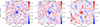 |
Fig. 2. Planck cleaned maps of SPT-CLJ0615-5746 of size |

3.2.2. SPT observations
Similary to the Planck maps, we used the public SPT maps, re-projected on smaller tiles of 1024 × 1024 pixels into the tangential plane, with a resolution of 0.5 arcmin/pixel (corresponding to ∼8.6° ×8.6°) around the X-ray peak of the cluster. We mask all point sources detected in the SPT maps, following the procedure detailed in Chown et al. (2018).
Due to the differences in frequencies and spatial scales covered, the SPT data are not compatible with the component separation technique explained in the previous section, which was specifically designed for the Planck data. Specifically, the SPT lacks high-frequency channels necessary for deriving the dust templates essential for the multi-component fit described earlier. Additionally, the noise level in the SPT’s 220 GHz channel is too high to accurately recover the CMB templates with the required precision. Without the templates to fit, Oppizzi et al. (2023) developed a new method tailored to the SPT data structure, including information from Planck to improve the reconstruction on larger spatial scales. Here we summarize the pipeline:
-
Similarly to what has been done in previous work (Delabrouille et al. 2009; Remazeilles et al. 2011; Hurier et al. 2013; Oppizzi et al. 2020), to recover the CMB signal, we started from a linear combination (LC) of the three SPT frequency maps and the 217 GHz map from Planck. Since the SPT window function changes with the channels, to make a LC of them, we first equalized the maps, including the Planck one, to the 150 GHz spatial response.
-
To combine maps from the two instruments with different resolution, we split each SPT map into a low-pass filtered map and a high-pass filtered map.
-
The LC weights are then calculated on a subregion of 1° ×1° around the X-ray peak, separately on the low- and high-pass maps (with the addition of the Planck map). In both cases, these are calculated as a double optimization: to minimize the variance with respect to a signal constant in frequency (CMB) and simultaneously to null the non-relativistic SZ component. These conditions lead to
 (2)
(2)where w are the weights assigned to each frequency, C is the data covariance matrix between the Nchan channels, e is a vector of lengths Nchan and A is the matrix accounting for the emission of the CMB and SZ signal at the various frequencies.
-
We recombined the CMB estimations of the large and small scales into a single map and rescaled to all SPT frequency to obtain the final templates.
-
Finally, we subtracted the templates from the SPT maps, obtaining the clean maps with the cluster signal.
Figure 3 shows the clean frequency maps that we use in the fit in Sect. 4.2.
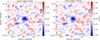 |
Fig. 3. SPT cleaned maps of SPT-CLJ0615-5746 of size |


4. Hot gas thermodynamics and profile fitting
With the case of SPT-CLJ0615-5746, we take advantage of the opportunity to validate the SZ profile fitting method at high redshifts and test if there is consistency between X-ray and millimetric data when incorporating Chandra data. In our analysis, we employed and compared two different fitting methods. The first approach involves the separate examination of the X-ray and millimeter observable. The second method incorporates a multiwavelength joint fit that combine data from three different instruments. This approach is designed to harness the strengths of each instrument and address potential systematic effects that may arise from the integration of Chandra data with SPT-Planck data, thereby providing a more robust and comprehensive analysis.
4.1. X-ray fit
The cluster emission from the hot plasma present in the ICM is modeled by combining the bremmsstrahlung continuum and the metal emission lines with the APEC spectral library and the absorption due to the Galactic medium. For the latter, we considered the photoelectric cross sections from Verner & Ferland (1996), the abundance table of Asplund et al. (2009). We considered the total hydrogen column density defined as the sum of the atomic hydrogen and the molecular contributions. We estimated this value directly from the X-ray spectrum of the cluster, considering a circular annulus with radii ![Mathematical equation: $ [0.15{-}0.8]\,R^{\mathrm{SPT}}_{500} $](/articles/aa/full_html/2024/08/aa49422-24/aa49422-24-eq28.gif) thus excluding the central regions. We performed the fit in the energy band [0.5 − 10.0] kev and left free to vary the total hydrogen column density, the temperature, the metallicity and the normalization of the spectrum. We find
thus excluding the central regions. We performed the fit in the energy band [0.5 − 10.0] kev and left free to vary the total hydrogen column density, the temperature, the metallicity and the normalization of the spectrum. We find  that is consistent with the value reported in the public data from the LAB survey (Kalberla et al. 2005) of NH = 4.32 × 1020 cm−2. Using the X-ray peak, we extracted the radial profiles of the background-subtracted X-ray observable: the surface brightness (ΣX) estimated in the soft X-ray band ([0.5, 2.5] keV) and the spectroscopic temperature (TX) considering the energy band [0.5, 10] keV. The former is defined as
 (3)
(3)
where x−1 = np/ne is the ionization factor, z is the redshift of the cluster and Λ(T, Z) is the cooling function of the cluster emission dependent on the temperature T and the element abundances Z. Surface brightness is expressed in detector units (photon counts cm−2 arcmin−2 s−1). For TX we assumed the temperature weighting scheme proposed in Mazzotta et al. (2004), to mimic the spectroscopic response of a single temperature,
 (4)
(4)
with  .
.
We then parameterized the emission measure [npne](r) using analytical forms first proposed in Vikhlinin et al. (2006)
![Mathematical equation: $$ \begin{aligned} n_{\rm p}n_{\rm e}(r)&= \frac{n_o^2(r/r_c)^{-\alpha }}{[1+(r/r_s)^{\gamma }]^{\epsilon /\gamma }[1+(r/r_c)^2]^{3\beta _1 -\alpha /2}} \nonumber \\&\quad + \frac{n_{0,2}^2}{[1+(r/r_{c,2})^2]^{3\beta _2}}\,, \end{aligned} $$](/articles/aa/full_html/2024/08/aa49422-24/aa49422-24-eq33.gif) (5)
(5)
where α is the cusp index accounting the higher densities in the cluster centre, n0 and n0, 2 are the normalization of two β-model profiles, with slopes β1 and β2 and characteristic radii rc and rc, 2, respectively. At large radii, ϵ represents the asymptotic change in slope near a given radius rs, with γ ruling the width of the transition region. For the temperature profile T(r), we used the functional form suggested in Vikhlinin et al. (2006)
![Mathematical equation: $$ \begin{aligned} T(r) = T_0 \frac{x+ T_{\rm min}/T_0}{x+1}\frac{(r/r_t)^{-a}}{[1+(r/r_t)^b]^{c/b}}\,, \end{aligned} $$](/articles/aa/full_html/2024/08/aa49422-24/aa49422-24-eq34.gif) (6)
(6)
where T0 is the overall normalization. The first ratio describes the decrease in temperature in the center as a function of the typical cooling scale x = (r/rcool)acool to a minimum temperature Tmin. The second is a broken power law, with characteristic scale rt and transition region describing the intermediate and outskirt profile of the cluster, with slope a, b and c.
These templates are then integrated along the line of sight and fitted to the two observable profiles (ΣX and TX). All fits are carried out with least-squares minimization following the Levenberg–Marquardt algorithm. For uncertainties envelopes of the best-fit profiles, we performed 500 parametric bootstrap realizations of the observed profiles, estimated considering 8 radial bins inside  for the spectroscopic temperature, and 25 logarithmic radial bins for the surface brightness inside
  . We show the surface brightness profile of our system in Fig. 4. The black dots represent the background subtracted data with their respective Poissonian statistical error associated with the measurement in each bin. The horizontal blue bar represents the background model with its 5% systematic error (details of the systematic errors associated with Chandra observations are in Bartalucci et al. 2014). The shaded red regions represent the sum of the statistical and systematic errors associated with the estimation of the background X-ray emission. In the last two bins we find that the emission measurements are more than 10 times below the background with the corresponding high dispersion, making the result for
  less reliable. Consequently, we do not employ the results beyond these radii in direct comparisons.
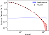 |
Fig. 4. Background-subtracted surface brightness profile of the Chandra data (black points) measured on SPT-CLJ0615-5746. The black bars represent the Poissonian statistical error associated with the measurement in each bin, while the shaded red regions represent the sum of the statistical and the 5% systematic error associated with the estimation of the background X-ray emission (shaded blue region). |
The decision to employ this radial range is motivated by our goal of derive the thermodynamic and hydrostatic mass profiles extending to the largest possible radii. However, at such high redshifts, obtaining a spectroscopic temperature measurement in the outer regions of the cluster presents a significant challenge. Specifically, we find that in the last two bins corresponding to ![Mathematical equation: $ [0.8,1.0]R^{\text{ SPT}}_{500} $](/articles/aa/full_html/2024/08/aa49422-24/aa49422-24-eq38.gif) and
and ![Mathematical equation: $ [1.0,1.4] R^{\text{ SPT}}_{500} $](/articles/aa/full_html/2024/08/aa49422-24/aa49422-24-eq39.gif) , the S/N is merely 12.4% and 5.4%, respectively. This implies that we lack sufficient photon counts to reliably infer the temperature in these regions. Consequently, we are unable to use the X-ray spectroscopic temperature data in the outermost portions of the cluster to extract our profiles.
, the S/N is merely 12.4% and 5.4%, respectively. This implies that we lack sufficient photon counts to reliably infer the temperature in these regions. Consequently, we are unable to use the X-ray spectroscopic temperature data in the outermost portions of the cluster to extract our profiles.
In this context, our primary goal is to constrain the X-ray density profile up to a high radial distance. To convert the emission measure profiles to gas density, we need the values of a factor that depend on temperature and element abundances (Λ(T, Z)). However, if the temperature is not well constrained, it may lead to inaccuracies in the brightness profile and consequently affect the accuracy of the density profile. To assess the sensitivity of the density profile to temperature variations at high radii, we conducted an analysis to evaluate how different temperature values in these outer regions can impact the final density profile. We deliberately manipulated the spectroscopic temperature values in the last two bins, creating three distinct scenarios: one with increasing temperature after  (represented by the black line in the left panel of Fig. 5), and two with decreasing temperatures with different gradients (shown as the blue and red lines in the left panel Fig. 5). We then performed the fit on the surface brightness profile using these different temperature profiles.
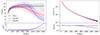 |
Fig. 5. Temperature and density profiles of SPT-CLJ0615-5746 obtained using different spectroscopic temperature values. Left: 3D temperature profiles for three different scenarios. The black line represents an increasing temperature in the outskirts, while the blue and red lines represent two decreasing temperatures with different gradients. Right: Respective density profile for each scenario. The shaded regions correspond to the 68% credible intervals. The bottom panels represent the relative deviation with respect to the increasing temperature (black profiles). |
The results of this test, as shown in the right panel of Fig. 5, indicate that even extreme temperature differences in the outer regions have a minimal impact, causing less than a 5% variation in the density profile within the same regions. This suggests that we can effectively constrain the density profile up to  without requiring precise knowledge of the exact temperature profile.
Finally, adopting a metal abundance constant normalization (Z = 0.3) for the cluster, the primordial helium abundance YP = 0.243 from Planck Collaboration VI (2020) results, and a particle mean weight of μ = 0.596 allowed us to infer an average ionization fraction np/ne = 0.852. We can use this value to infer the electronic density distribution ne(r), from the parametric form of [npne](r) (Eq. (5)). The upper left panels of Fig. 10 shows the best-fit deprojected 3D density profile with its corresponding 68% uncertainty envelope.
4.2. Millimetric fit
To probe the gas pressure structure in both the inner and outer cluster regions, we combined the SPT and Planck data in a joint fit. We first assume that the pressure structure follows the spherically symmetric profile proposed by Nagai et al. (2007)
 (7)
(7)
where x = c500r/R500, while γ and β are the slopes at r ≪ R500/c500, and r ≫ R500/c500 respectively. Here, α can be better understood as quantification of the sharpness of the transition between the rγ and the rβ regimes. To fit the millimetric data, P(r) is used to build the thermal SZ signal expected for each channel in both Planck and SPT. We projected the 3D profile along the line of sight, and then converted in SZ brightness:
 (8)
(8)
The sSZ,c coefficients that represent the frequency scaling, are derived from the non-relativistic Kompaneets equation
![Mathematical equation: $$ \begin{aligned} s_{\text{ SZ,c}}=\int \,\mathrm{d}\nu \,R_c(\nu )x(\nu )\Bigg [\frac{e^{x_{\nu }}+1}{e^{x_{\nu }}-1}-4\Bigg ]\,, \end{aligned} $$](/articles/aa/full_html/2024/08/aa49422-24/aa49422-24-eq44.gif) (9)
(9)
where x(ν)=hν/kT, while Rc(ν) define the channel spectral response that for Planck is given by the HFI model (Planck Collaboration XLIII 2016). For SPT the spectral response is given in Chown et al. (2018).
For Planck observations we also added a correction term to take into account the CTD component, that has been observed in Planck data ,collaborartion2016planck; (Planck Collaboration XLIII 2016).
The complete model is then applied to fit the frequency maps from both SPT and Planck to derive the amplitudes of the templates and contaminant components on a channel-by-channel basis while marginalizing over the cluster signal. Clean cluster maps, obtained by differencing the background and foreground templates, are used for this fitting process.
For each cleaned map we calculated the radial SZ profiles centered on the X-ray peak. Profile values are calculated by averaging over the pixels whose centers fall within the annulus defined by the bin edges. We employ 11 bins up to  for SPT and 8 bins up to
  for Planck. This binning scheme ensures that the first bin has a size exceeding 0.5 arcmin for SPT and 1 arcmin for Planck.
In our analysis, we used the 95 and 150 GHz channels of SPT and the 100, 143, and 353 GHz channels of Planck. The other channels are still used in the component separation process, but are not included in the fit itself. This approach is motivated by the low signal-to-noise ratio of the cluster signals expected at these frequencies. By excluding them, we enhance computational efficiency with minimal loss of information and reduce the risk of residual contamination from dominant dust emission in these channels.
We compared the model with the data using the likelihood
 (10)
(10)
where lnℒSZ(θ) is the Gaussian log-likelihood associated with the SZ profiles yi and the associated template ISZ, i obtained integrating the Pressure profile in Eq. (7) with parameters θ = [P0, c500, α, β, γ]. Since we reconstruct the SPT CMB using a linear combination of different channels, there is a possibility that noise from one map might inadvertently affect the others during the background subtraction process. To account for this, we computed the two covariance matrices Ci, for both SPT and Planck. We generated 100 profiles from the cleaned maps in regions where we applied the same cleaning technique, but we did not expect the presence of cluster signals. For both instruments, we concatenated the profiles derived from each map and calculated the covariance among all these profiles. This approach ensures that the covariance accounts for both instrumental noise and correlations between channels. However, it is important to note that we considered SPT and Planck channels to be uncorrelated with each other.
We employed the Cobaya MCMC (Torrado & Lewis 2021) framework to perform the fit and uncertainty estimation, exploring various combinations of parameters to optimize the convergence of our chains. However, to constrain the shape of the pressure profile from the inner regions to the faint outskirts of the cluster, we allowed three parameters to vary freely: the amplidude P0, the inner slope γ and the outer slope β. The other two parameters are held fixed at their universal values (Arnaud et al. 2010): c500 = 1.177 and α = 1.051. We employed uniform priors in combination with the likelihood to estimate the posterior distribution. Due to the limited resolution of both SPT and Planck, the correlation between P0 and γ poses a challenge, as both parameters describe the internal regions of the cluster. To address this, strict priors on γ are necessary to achieve the convergence of the chain. However, even with these precautions, the divergence between the two parameters persists, and obtaining proper constraints on both parameters remains challenging. The only effective approach to achieve both convergence in the chains and obtain reliable constraints on the parameters is to also fix γ = 0.3081 to its universal value from Arnaud et al. (2010).
4.3. Joint X-ray and millimetric fit
Our goal is to obtain comprehensive thermodynamic profiles and the hydrostatic mass for this high-redshift system, extending our analysis to larger radii. However, as detailed in Sect. 4.1, constraining the spectroscopic temperature in the outermost regions of the cluster at such high redshift poses a significant challenge. To overcome this limitation, we intend to merge the density profile from the X-ray fitting with the pressure profile derived from the millimetric analysis. This combined approach allows us to extract the remaining thermodynamic profiles, even in these outer regions.
Nevertheless, combining information from instruments with distinct resolutions, such as X-ray and SZ observations, can introduce various systematic uncertainties into our analysis. As explained in previous studies (Bourdin et al. 2017; Kozmanyan et al. 2019; Wan et al. 2021, De Luca et al., in prep.), although both methods probe the same gas, discrepancies can arise between X-ray-only and SZ-only analyses. The sources of these differences can be attributed to the geometry of the system, calibration uncertainties of the instruments, or due to the underlying cosmological framework. To account for the possibility of such systematic effects, we introduce a free normalization parameter, denoted ηT, which scales the X-ray and millimeter inferences of the ICM profiles accordingly. In the ideal scenario, we would expect ηT = 1, but in more realistic cases ηT is expected to deviate from one due to the various factors mentioned earlier. As detailed in Kozmanyan et al. (2019), ηT has a straightforward dependence on these properties and can be expressed as a product of three terms:
 (11)
(11)
The first term relates to quantities tied to the cosmological model. X-ray and SZ signals for a given cluster exhibit different dependencies on the cosmic distance from the cluster’s redshift. The X-ray density depends on the ICM emissivity, thus involves factors of the angular diameter distance, DA(z), in particular ne ∝ DA(z)−3/2 (Mantz et al. 2014). In contrast, the SZ signal is proportional to the integral along the line of sight of the electron pressure, and thus PSZ ∝ DA(z)−1. Combining the two different dependencies, we get 𝒞 ∝ DA(z)1/2. Additionally, the X-ray surface brightness is influenced by the chemical composition of the gas, predominantly hydrogen and helium. This dependence in Eq. (3) comes from the cooling function Λ(T, Z). Assuming negligible contributions from other elements to the X-ray continuum, we can express the contribution of hydrogen and helium separately Λ(T, H, Y)∝ΛH × (1 + 4nHe/np). This introduces an additional cosmological bias dependent on the value of the helium abundance Y, which is added to the cosmological part of the normalization parameter. The total cosmological systematic can be parameterized as 𝒞 ∝ DA(z)−1/2 × Y−1/2.
The second term of Eq. (11) encapsulates any morphological bias resulting from the geometry of the system. Throughout our analysis, we assume perfect spherical symmetry. Given that the X-ray and SZ signals have different dependencies on density, an eventual asphericity would affect the normalization parameter. Moreover, more realistic gas distributions may include clumpiness, which, like asphericity, would enhance the X-ray emission of the cluster. Taking into account these factors, the geometric part of the normalization parameter can be expressed as  , where eLOS and Cρ account for cluster asphericity (for details regarding the parameterization of this parameter, refer to De Filippis et al. 2005; Sereno et al. 2006) and clumpiness, respectively. For detailed derivations of the dependence of the cosmological and geometrical systematic, refer to Kozmanyan et al. (2019). The last term accounts for all other potential systematics due to uncertainties in the calibration of X-ray spectroscopic temperature, since a variation in temperature for the cluster results in a variation in the normalization parameter in the same direction. Finally, other potential biases may be associated with assumptions and approximations in our methodology, such as profile modeling or the fitting procedure.
To conduct our joint X-ray and millimetric fit, we need to account for all the potential systematic effects described above, encapsulated within the normalization parameter. We used the pressure profile from Eq. (7) to construct both the SZ brightness template (as defined in Eq. (8)) and a spectroscopic temperature template derived from the ideal gas law:
 (12)
(12)
Here, we fixed ne(r) to the form obtained in Sect. 4.1. We fitted this template to two projected X-ray temperatures extracted in ![Mathematical equation: $ [0.0-0.15]R^{\text{ SPT}}_{500} $](/articles/aa/full_html/2024/08/aa49422-24/aa49422-24-eq51.gif) and
and ![Mathematical equation: $ [0.15-0.8]R^{\text{ SPT}}_{500} $](/articles/aa/full_html/2024/08/aa49422-24/aa49422-24-eq52.gif) , ensuring that we have a S/N that exceeds 30% in both bins.
, ensuring that we have a S/N that exceeds 30% in both bins.
As detailed in Sect. 4.2, we performed the fit using the Cobaya MCMC framework, allowing the parameters P0, β, γ and the normalization parameter ηT to vary freely. After obtaining the best-fit parameters through joint X-ray and millimetric fit, we employed Eq. (7) to derive the pressure profile PSZ,X = ηTP(r). This pressure profile provides valuable information about the thermodynamics of the galaxy cluster, enabling us to further explore its properties and derive other relevant profiles.
5. Results
5.1. Parametric modeling and pressure profile
Figure 6 shows the outcomes of our joint fit procedures applied to the SZ radial frequency profiles obtained from both the SPT and Planck channels used in our analysis. These profiles are presented alongside the background and foreground components. We calculated the best-fit profile (blue lines) using the set of parameters that maximize the likelihood of our chains. As shown in the off-diagonal panels of Fig. 7 our joint fit approach, which combines X-ray and millimetric data, improves the constraint on the profile parameters Nagai et al. (2007), particularly by alleviating the degeneracy between P0 and γ and providing better constraints on the posterior distribution of the internal shape. This, in turn, results in a more accurate constraint on the other two parameters. This improvement is mainly attributed to the high spatial resolution of the Chandra telescope, allowing better constraints on the shape of the pressure profile within the inner region of the cluster (inside  ).
).
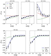 |
Fig. 6. Radial profile of the SZ brightness around the X-ray peak of SPT-CLJ0615-5746 of the Planck (upper panels) and SPT (lower panels) channels used in the fitting procedure. The black dots represent the radial average values on the cleaned maps with their respective errors, and the green and brown lines represent the CMB and GTD. The blue line represents the best fit from the joint X-ray and millimetric analysis (Sect. 4.3). The vertical dashed lines indicate the FWHM of the beam in each frequency channel. |
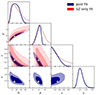 |
Fig. 7. Corner plot illustrating the results of the MCMC analysis for the Nagai et al. (2007) model parameters and the normalization parameter. The joint fit is represented by the blue lines and contours, while the red lines represent the SZ-only fit. Each panel along the diagonal displays the marginalized posterior distribution for a single parameter, while the off-diagonal panels show the two-dimensional projections highlighting the covariances between parameter pairs. The contours represent the 68% and 95% confidence intervals. There is no red counterpart for the ηT parameter since it is not fitted in the SZ-only fit. The white crosses represent the position of the best-fit (maximum likelihood) parameters associated with the joint fit. |
Although the joint-fitting approach clearly enhances our ability to constrain the pressure structure within the inner regions of the cluster, it is worth noting that we obtain a relatively high value for the normalization parameter. In particular, we find that the best fit that maximizes our likelihood is  where the intervals represent the 16th and 84th percentiles. This value implies that, for this particular system, there is a significant difference of around 50% between the ICM properties derived from our X-ray analysis and those obtained through the SZ analysis. Despite the relatively high value obtained, our findings reveal a lower result compared to the value reported in Bourdin et al. (2017). In their study, they performed a joint fit using Chandra and Planck-only data sets for this particular cluster, producing a value of ηT ∼ 1.7. These outcomes suggest that the inclusion of SPT data in the joint fit effectively reduces the systematics observed between the X-ray and millimeter data sets. This reduction can be attributed to the higher resolution provided by SPT in contrast to Planck, enabling the analysis of pressure structures at radii closer to the X-ray resolution.
We compare the ηT values obtained from our joint fit with the median values of the parameter distributions derived with similar joint X-ray and millimetric analysis. Bourdin et al. (2017) conducted a joint Planck-Chandra analysis of clusters with z > 0.5, yielding median values of the normalization parameter:  . Similarly, Wan et al. (2021), combined Chandra, Planck, and Bolocam data for 14 clusters with 0.07 < z < 0.55, finding a median ℛ value (equivalent of the ηT parameter) of 1.13 ± 0.09. Compared to the median Chandra results, our analysis for this individual system leads to higher values of the parameter.
To compare our findings with studies based on XMM-Newton, we consider the known temperature discrepancies between Chandra and XMM-Newton. Although the existence of this discrepancy does not provide information on the correct absolute calibration, on average, Chandra temperatures are ∼10 − 15% higher than those from XMM-Newton (Nevalainen et al. 2010; Schellenberger et al. 2015), consequently increasing the ηT parameter by the same amount. Even after considering these factors, our values still lie outside of the ∼10% scatter around unity in the ηT distribution found with XMM-Newton:  (Bourdin et al. 2017);
  (Kozmanyan et al. 2019); ηT = 0.96 ± 0.08 (Ghirardini et al. 2019); 0.98 ± 0.02 (De Luca et al., in prep.). These comparisons further confirm the aspherical nature of the gas halo in this particular system.
5.2. Angular sectors
As explained in Sect. 4.3, the ηT parameters is influenced primarily by two factors: one associated with the underlying cosmological framework and the other related to the properties of the ICM distribution. To separate the contributions of these two factors, we considered the possibility of the cluster deviating from spherical symmetry. This assumption is motivated by our analysis of the surface brightness map of the cluster, as illustrated in Fig. 1. This map reveals a departure from perfect sphericity, displaying an elliptical-like shape that is not visible in the SPT and Planck maps due to their lower angular resolutions.
In this section, we followed the methodology detailed in Sect. 4.1 to derive two separate density profiles for sectors aligned with the cluster’s minor and major axes. Figure 8 visually represents the specific regions from which we extracted the surface brightness profile. The regions identified by number one are associated with the circular sector along the minor axis, while the remaining regions correspond to the major axis. To facilitate this analysis, we applied masks to the opposing regions, ensuring that only photon counts within each sector were considered. Subsequently, the two density profiles are employed in Eq. (12) to perform the joint fit for the major and minor axes. We left the SZ analysis unchanged, which means that we did not perform the same division for the SZ profiles. In this way, we introduced an additional geometrical bias that would affect the ηT parameter. The best-fit parameters with with the 16th and 84th percentiles of the distributions are shown in Table 2. The MCMC results of the joint fit applied on the two sectors are shown in Fig. 9. Our analysis yields  and
and  for the minor and major axes, respectively. This discrepancy can be attributed to the elliptical shape of the cluster, since at higher radii the density measured along the major axis is higher than the one along the minor axis, with the total one being the mean between the two, as shown in the top left panels of Fig. 10. These results confirm that a portion of the discrepancies between the X-ray and SZ analyses can be attributed to geometrical effects specific to this system. Moreover, in our joint fit the ηT parameter comes from Eq. (12), which becomes
 (13)
(13)
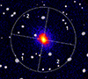 |
Fig. 8. X-ray Chandra image after background subtraction, captured within the energy range of [0.5,2.5] keV. The dashed white circle denotes the position at a radius of |

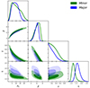 |
Fig. 9. Corner plot illustrating the results of the MCMC analysis for the Nagai et al. (2007) model parameters and normalization parameter for our sector-based analysis. The minor axis results are denoted by green lines and contours, while results for the major axis are shown in light blue. Each panel along the diagonal displays the marginalized posterior distribution for a single parameter, while the off-diagonal panels show the two-dimensional projections highlighting the covariances between parameter pairs. The contours represent the 68% and 95% confidence intervals. |
Best-fit parameters along with the 16th and 84th percentiles of the posterior distributions for the Nagai et al. (2007) and ηT parameters.
Since we used the same two spectroscopic temperatures bins (red points in Fig. 10) in the three regions and the SZ analysis is unchanged, the ηT parameter adjusts accordingly to compensate for differences in the density profile. This leads to a lower value for the minor axis and a higher value for the major axis.
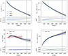 |
Fig. 10. Thermodynamic profiles of SPT-CLJ0615-5746 for both total and angular sectors analysis. Top: Density and pressure profiles derived independently from the X-ray analysis and the joint fit, respectively. Bottom left: 3D temperature profile derived from the ideal gas law. The red points represent the spectroscopic temperature bins used in the joint fit. The brown dotted line shows the 3D temperature from Bartalucci et al. (2017), derived from a deprojection of the X-ray spectroscopic temperatures of this system. Bottom right: Cluster entropy profile derived from Eq. (15). The violet dotted line shows the theoretical entropy profiles from the gravity-only simulations of Voit et al. (2005). In each figure the black solid line represents the profile derived from the total density profile, while the green and blue lines represent the analysis conducted along the minor and major axes, respectively. The dashed section line marks the region inside the innermost Chandra spectroscopic temperature data point. The vertical dashed line represents the estimation of |

Toward the end of our fitting procedure, we obtained two radial profiles for both the total and the angular sector analysis : the density profiles from the Chandra X-ray fit and pressure profiles from the joint X-ray and millimetric fit, represented as PSZ,X(r)=ηTP(r) (top panels of Fig. 10). For our analysis, we considered a radial range spanning from approximately  up to around
  . The upper limit is determined by the emission mesure from Chandra analysis, where the signal becomes undetectable on the edges of the cluster, as ΣX scales with
  . On the contrary, the lower limit is dictated by the first spectroscopic temperature bin used in the joint fit. Ultimately, we combine these profiles to unravel the thermodynamic properties of the gas of the galaxy cluster and the hydrostatic mass.
5.3. Temperature and entropy profiles
Assuming that the gas behaves as an ideal gas, we can use the Eq. (12) to recover the 3D temperature profile kTSZ, X(r) and the ICM entropy profile KSZ, X from the following equations:
 (14)
(14)
 (15)
(15)
By combining the two data sets, we are able to determine the 3D temperature and entropy profiles up to radial distances beyond  without the need for extrapolating a parametric temperature profile in regions where the spectroscopic temperature is not well constrained.
The profiles obtained are presented in the lower panels of Fig. 10. Remarkably, we observe a high level of agreement with the 3D temperatures derived from an X-ray-only analysis, as reported in Bartalucci et al. (2017), within the range covered by their radii. These findings emphasize the consistency and robustness of our joint fit method, enabling the extraction of thermodynamic profiles up to higher radii in comparison to an X-ray-only analysis.
Moreover, also our entropy profiles are consistent with the expected profile of Voit et al. (2005). Here, we highlight that our method is mostly limited by our ability to extract a density profile regardless of the availability of spectroscopic temperature measurements.
Alongside the total profiles (black lines) we show the results obtained from our angular sector-based analysis (green and blue lines). The temperature profiles are computed using Eq. 14, along with the density profiles extracted in the three regions. Since our joint fit leads to a constant ratio ηT/ne(r), we get the same 3D temperature profiles regardless of where we extract the emission measure data to fit the density profile. This does not apply for the entropy profiles. From Eq. (15) it is clear that density plays a more dominant role compared to pressure, leading to differences (within the errors) between our sector-based profiles on the outskirts of the cluster.
5.4. Hydrostatic mass profile
Under the assumption of spherical symmetry and hydrostatic equilibrium, the integrated mass profile of a galaxy cluster can be expressed as
 (16)
(16)
where μ = 0.596 is the gas mean molecular weight, G is the Newton’s constant and mp is the proton mass. We extract the hydrostatic mass profile by combining the pressure profile measured from our joint fit PSZ, X = ηTP(r) and the density profile ne(r) measured independently from the X-ray data. Combining the two profiles, we get
 (17)
(17)
Given that we can constrain the pressure profile from the SZ signal to distances greater than 2 R500, the upper limit of our hydrostatic mass estimation is determined by the radial range covered by the density profile. Figure 11 displays the results of our analysis, showing the mass profiles derived from our calculations. Using the critical density of the Universe at the cluster’s redshift, we calculate the over-density contrast by integrating the mass profile. This enables the determination of  (vertical dashed line of Fig. 11), from which we subsequently compute
  .
.
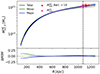 |
Fig. 11. Mass profiles of SPT-CLJ0615-5746, derived under the assumption of hydrostatic equilibrium using Eq. (17). The black solid line represents the mass profile derived from the total density profile, while the green and blue lines represent the analysis conducted along the minor and major axes, respectively. The dashed section line marks the region inside the innermost Chandra spectroscopic temperature data point. The vertical dashed line represents the estimate |


We also present hydrostatic mass estimations for our analysis based on the angular sector. Profiles are calculated using Eq. (17), which incorporates the density profiles extracted from the three regions. Similarly to 3D temperature profiles, the constant ratio ηT/ne(r) ensures consistent hydrostatic mass measurements regardless of the region considered.
Our findings indicate that the stability and consistency of our mass and temperature estimates persist, regardless of the chosen region for extracting emission measure data to fit the density profile. This implies that variations in the normalization parameter, whether higher or lower, effectively compensate for any differences in the density profile.
We compare the hydrostatic mass estimates obtained from our joint fit with other mass estimates derived from independent studies or methods. To make a meaningful comparison, we interpolated our mass profiles at the radii corresponding to the locations of the other mass estimates. Despite the elongated shape of this system, we find good agreement with the integrated mass estimation based on the M500 − YSZ and M500 − ξ scaling relations. In particular, our result aligns with the ξ-mass scaling relation used in the SPT catalog (Bleem et al. 2015). We find  (
( is interpolated at
  ). Furthermore, we compared our hydrostatic mass estimate with the integrated mass estimate of the YX proxy. We calculated the value of
  and
and  iteratively using the M500 − YX scaling relation calibrated with estimates from Chandra data (Vikhlinin et al. 2009). Here YX is defined as the product of the gas mass computed at
  and the temperature measured in
 ![Mathematical equation: $ [0.15{-}1.0]\,R^{Y_{X}}_{500} $](/articles/aa/full_html/2024/08/aa49422-24/aa49422-24-eq96.gif) . Finally, we compared our two estimates by interpolating the hydrostatic mass at
. Finally, we compared our two estimates by interpolating the hydrostatic mass at  . In this case, also, we find excellent agreement with
  .
.
Finally, we compared our results with the X-ray only hydrostatic mass published in Bartalucci et al. (2018) who determined  for this cluster, combining XMM-Newton and Chandra observations. In particular, we find
  , where
  is interpolated at
  . An X-ray only estimates of
  of such high redshift cluster are possible thanks to the deep Chandra observations available for this system, since it relies on the radial coverage provided by temperature data. The consistency between our mass and an X-ray only mass estimates provides confidence in extending trust to our results at larger radii, where we do not have enough statistics to constrain the spectroscopic temperatures. These findings suggest the potential extension of our analysis to clusters where we do not have such deep observation, encouraging us to apply our method even to higher-redshift clusters.
6. Summary and conclusions
In this paper we introduced a multiwavelength technique to resolve the gas properties of the most distant galaxy cluster detected by Planck, located at z = 0.972. Our approach combined data from Planck and the South Pole Telescope (SPT) with Chandra observations, and allowed us to extract individual pressure and density profiles for this cluster up to R > R500. We employed two distinct fitting methods. The first involves independent analyses of the data from Chandra and SPT-Planck (SZ-only) data. In contrast, the second method employs a joint fit that combines the multiwavelength data from all three instruments. For the latter, we introduced a free normalization parameter ηT to build a temperature template. This template was then fitted exclusively in the innermost region of the cluster R < 0.8 R500, where there are enough photons count to constrain the spectroscopic temperatures. Our main findings and results regarding our fitting methods are summarized below:
-
Our multiwavelength approach allows us to constrain the thermodynamic profiles across a wider range of spacial scales compared to a SZ-only or X-ray-only analysis. The high resolution provided by Chandra facilitates a more precise constraint on the shape of the pressure profile within the inner region of the cluster. Meanwhile, the synergy between SPT and Planck allows us to extend these constraints to larger spatial scales. The reduced uncertainty in the shape of the profile translates into improved accuracy in determining the best-fit parameters of the Nagai et al. (2007) profile.
-
Our analysis reveals a high value for the normalization parameter, specifically
 . We observe a significant deviation from the ideal case (ηT = 1) , and this holds whether we extract the density in concentric rings or in sectors along the principal axes. Even when using the latter approach, which helps mitigate geometric effects due to the departure of this system from spherical symmetry, we still obtain ηT > 1. The discrepancy in the values of ηT suggests that a straightforward combination of Chandra X-ray and millimetric data, without accounting for systematic differences, is not feasible. This highlights the importance of incorporating a normalization parameter in our analysis, as it encodes these systematics comprehensively.
We then combined the resulting profile from our fitting procedure to calculate the hydrostatic mass, 3D temperature, and entropy profiles up to R > R500 without the need for precise spectroscopic temperature measurements in the outskirts of the cluster. Here are the main results:
-
Our multiwavelength approach allows us to extend our coverage to a radial range primarily limited by our ability to extract a density profile rather than by the availability of spectroscopic temperature measurements. This highlights the potential of our method to provide insights into thermodynamic profiles and hydrostatic mass of galaxy clusters at large radii, even in cases where obtaining accurate spectroscopic temperature data is challenging.
-
Our 3D temperature profile aligns with the X-ray-only analysis conducted in Bartalucci et al. (2017), specifically within the range covered by their radii. This consistency ensures the robustness of our analysis, providing confidence in extending trust to the results at larger scales.
-
We find that the hydrostatic mass and temperature estimates remain stable and consistent, regardless of the region-specific density profiles used. The variation in the normalization parameter effectively compensates for the differences between the X-ray and millimetric selected regions of the cluster, resulting in similar mass estimate.
-
We compare our value of
 with other estimates. In particular, we find a good alignment with the ξ-mass scaling relation used in the SPT catalog (Bleem et al. 2015) and with the M500 − YX scaling relation (Vikhlinin et al. 2009). We also find consistency with the hydrostatic mass estimates based only on X-rays from Bartalucci et al. (2018).
This study represents the initial comprehensive application of the methodology developed in Bourdin et al. (2017) and Oppizzi et al. (2023) to investigate and resolve the ICM properties of high-redshift objects. We successfully combined data from three different instruments, allowing us to analyze a broad radial range of the cluster. Chandra and SPT provide insights into the cluster structure up to the inner regions (approximately 0.15 R500), while the Planck data serve as a robust anchor at larger angular scales and provide improved estimates of the cosmic microwave background and the galactic thermal dust emissions.
The introduction of a normalization parameter offers several advantages. First, it exploits the synergy between X-ray and mm observations by resolving cluster cores close to an arc-second angular resolution while probing cluster peripheries out to intra-cluster radii barely accessible to X-ray spectroscopy alone. Moreover, it highlights the systematic uncertainties arising from the combination of different instruments. Our work demonstrates the power of combining multiwavelength observations to obtain a comprehensive understanding of galaxy clusters. This technique opens up new possibilities for studying the gas properties and mass distribution in clusters even when spectroscopic temperature measurements are challenging to obtain, in particular, for high redshift clusters. For distant galaxy clusters of SZ cluster catalogs also observed in X-rays, these results motivate future studies related to the evolution with cosmic times of the hot gas thermodynamics and the shape of matter haloes.
Acknowledgments
CM, FO, HB, PM, and FDL acknowledge financial contribution from the contracts ASI-INAF Athena 2019-27-HH.0, “Attività di Studio per la comunità scientifica di Astrofisica delle Alte Energie e Fisica Astroparticellare” (Accordo Attuativo ASI-INAF n. 2017-14- H.0), from the European Union’s Horizon 2020 Programme under the AHEAD2020 project (grant agreement n. 871158), support from INFN through the InDark initiative, from “Tor Vergata” Grant “SUPERMASSIVE-Progetti Ricerca Scientifica di Ateneo 2021”, and from Fondazione ICSC , Spoke 3 Astrophysics and Cosmos Observations. National Recovery and Resilience Plan (Piano Nazionale di Ripresa e Resilienza, PNRR) Project ID CN00000013 ‘Italian Research Center on High-Performance Computing, Big Data and Quantum Computing’ funded by MUR Missione 4 Componente 2 Investimento 1.4: Potenziamento strutture di ricerca e creazione di “campioni nazionali di R&S (M4C2-19 )” – Next Generation EU (NGEU). We acknowledge the financial contribution from the contract Prin-MUR 2022 supported by Next Generation EU (n.20227RNLY3 The concordance cosmological model: stress-tests with galaxy clusters).
References
- Adam, R., Ricci, M., Eckert, D., et al. 2024, A&A, 684, A18 [NASA ADS] [CrossRef] [EDP Sciences] [Google Scholar]
- Arnaud, M., Pratt, G., Piffaretti, R., et al. 2010, A&A, 517, A92 [CrossRef] [EDP Sciences] [Google Scholar]
- Asplund, M., Grevesse, N., Sauval, A. J., & Scott, P. 2009, ARA&A, 47, 481 [NASA ADS] [CrossRef] [Google Scholar]
- Bartalucci, I., Arnaud, M., Pratt, G., et al. 2017, A&A, 598, A61 [NASA ADS] [CrossRef] [EDP Sciences] [Google Scholar]
- Bartalucci, I., Mazzotta, P., Bourdin, H., & Vikhlinin, A. 2014, A&A, 566, A25 [NASA ADS] [CrossRef] [EDP Sciences] [Google Scholar]
- Bartalucci, I., Arnaud, M., Pratt, G. W., & Le Brun, A. 2018, A&A, 617, A64 [NASA ADS] [CrossRef] [EDP Sciences] [Google Scholar]
- Bertin, E., & Arnouts, S. 1996, A&AS, 117, 393 [NASA ADS] [CrossRef] [EDP Sciences] [Google Scholar]
- Bleem, L., Stalder, B., De Haan, T., et al. 2015, ApJS, 216, 27 [NASA ADS] [CrossRef] [Google Scholar]
- Bleem, L. E., Klein, M., Abbot, T. M. C., et al. 2024, Open J. Astrophys., 7, 13 [CrossRef] [Google Scholar]
- Bourdin, H., & Mazzotta, P. 2008, A&A, 479, 307 [NASA ADS] [CrossRef] [EDP Sciences] [Google Scholar]
- Bourdin, H., Mazzotta, P., Markevitch, M., Giacintucci, S., & Brunetti, G. 2013, ApJ, 764, 82 [Google Scholar]
- Bourdin, H., Mazzotta, P., Kozmanyan, A., Jones, C., & Vikhlinin, A. 2017, ApJ, 843, 72 [Google Scholar]
- Chown, R., Omori, Y., Aylor, K., et al. 2018, ApJS, 239, 10 [Google Scholar]
- Connor, T., Kelson, D. D., Blanc, G. A., & Boutsia, K. 2019, ApJ, 878, 66 [NASA ADS] [CrossRef] [Google Scholar]
- Curry, H. B., & Schoenberg, I. J. 1965, On polya frequency functions IV: The fundamental Spline functions and their limits., Tech. rep., Wisconsin Univ Madison Mathematics Research Center [Google Scholar]
- De Filippis, E., Sereno, M., Bautz, M. W., & Longo, G. 2005, ApJ, 625, 108 [NASA ADS] [CrossRef] [Google Scholar]
- Delabrouille, J., Cardoso, J.-F., Le Jeune, M., et al. 2009, A&A, 493, 835 [NASA ADS] [CrossRef] [EDP Sciences] [Google Scholar]
- Finkbeiner, D. P., Davis, M., & Schlegel, D. J. 1999, ApJ, 524, 867 [NASA ADS] [CrossRef] [Google Scholar]
- Garmire, G. P., Bautz, M. W., Ford, P. G., Nousek, J. A., & Ricker, G. R., Jr 2003, SPIE, 4851, 28 [Google Scholar]
- Ghirardini, V., Eckert, D., Ettori, S., et al. 2019, A&A, 621, A41 [NASA ADS] [CrossRef] [EDP Sciences] [Google Scholar]
- Hurier, G., Macías-Pérez, J., & Hildebrandt, S. 2013, A&A, 558, A118 [NASA ADS] [CrossRef] [EDP Sciences] [Google Scholar]
- Jiménez-Teja, Y., Dupke, R. A., Lopes, P. A. A., & Vílchez, J. M. 2023, A&A, 676, A39 [NASA ADS] [CrossRef] [EDP Sciences] [Google Scholar]
- Kalberla, P. M., Burton, W., Hartmann, D., et al. 2005, A&A, 440, 775 [NASA ADS] [CrossRef] [EDP Sciences] [Google Scholar]
- Kozmanyan, A., Bourdin, H., Mazzotta, P., Rasia, E., & Sereno, M. 2019, A&A, 621, A34 [NASA ADS] [CrossRef] [EDP Sciences] [Google Scholar]
- Mantz, A. B., Allen, S. W., Morris, R. G., et al. 2014, MNRAS, 440, 2077 [NASA ADS] [CrossRef] [Google Scholar]
- Mazzotta, P., Rasia, E., Moscardini, L., & Tormen, G. 2004, MNRAS, 354, 10 [NASA ADS] [CrossRef] [Google Scholar]
- Meisner, A. M., & Finkbeiner, D. P. 2014, ApJ, 798, 88 [NASA ADS] [CrossRef] [Google Scholar]
- Nagai, D., Kravtsov, A. V., & Vikhlinin, A. 2007, ApJ, 668, 1 [Google Scholar]
- Nevalainen, J., David, L., & Guainazzi, M. 2010, A&A, 523, A22 [NASA ADS] [CrossRef] [EDP Sciences] [Google Scholar]
- Oppizzi, F., Renzi, A., Liguori, M., et al. 2020, J. Cosmol. Astropart. Phys., 2020, 054 [CrossRef] [Google Scholar]
- Oppizzi, F., De Luca, F., Bourdin, H., et al. 2023, A&A, 672, A156 [NASA ADS] [CrossRef] [EDP Sciences] [Google Scholar]
- Planck Collaboration XXIII. 2016, A&A, 594, A23 [NASA ADS] [CrossRef] [EDP Sciences] [Google Scholar]
- Planck Collaboration XXVI. 2016, A&A, 594, A26 [NASA ADS] [CrossRef] [EDP Sciences] [Google Scholar]
- Planck Collaboration XXVII. 2016, A&A, 594, A27 [NASA ADS] [CrossRef] [EDP Sciences] [Google Scholar]
- Planck Collaboration XLIII. 2016, A&A, 596, A104 [NASA ADS] [CrossRef] [EDP Sciences] [Google Scholar]
- Planck Collaboration VI. 2020, A&A, 641, A6 [NASA ADS] [CrossRef] [EDP Sciences] [Google Scholar]
- Remazeilles, M., Delabrouille, J., & Cardoso, J.-F. 2011, MNRAS, 418, 467 [Google Scholar]
- Ruppin, F., McDonald, M., Bleem, L., et al. 2021, ApJ, 918, 43 [NASA ADS] [CrossRef] [Google Scholar]
- Schellenberger, G., Reiprich, T., Lovisari, L., Nevalainen, J., & David, L. 2015, A&A, 575, A30 [NASA ADS] [CrossRef] [EDP Sciences] [Google Scholar]
- Schrabback, T., Applegate, D., Dietrich, J., et al. 2018, MNRAS, 474, 2635 [NASA ADS] [CrossRef] [Google Scholar]
- Sereno, M., De Filippis, E., Longo, G., & Bautz, M. W. 2006, ApJ, 645, 170 [NASA ADS] [CrossRef] [Google Scholar]
- Starck, J.-L., Pantin, E., & Murtagh, F. 2002, PASP, 114, 1051 [NASA ADS] [CrossRef] [Google Scholar]
- Starck, J.-L., Fadili, J., & Murtagh, F. 2007, IEEE Trans. Image Proc., 16, 297 [Google Scholar]
- Starck, J.-L., Fadili, J. M., Digel, S., Zhang, B., & Chiang, J. 2009, A&A, 504, 641 [NASA ADS] [CrossRef] [EDP Sciences] [Google Scholar]
- Sunyaev, R., & Zeldovich, Y. B. 1972, Comm. Astrophys. Space Phys., 4, 173 [Google Scholar]
- Torrado, J., & Lewis, A. 2021, J. Cosmol. Astropart. Phys., 2021, 057 [CrossRef] [Google Scholar]
- Verner, D. A., & Ferland, G. J. 1996, ApJS, 103, 467 [NASA ADS] [CrossRef] [Google Scholar]
- Vikhlinin, A., Kravtsov, A., Forman, W., et al. 2006, ApJ, 640, 691 [Google Scholar]
- Vikhlinin, A., Kravtsov, A., Burenin, R., et al. 2009, ApJ, 692, 1060 [CrossRef] [Google Scholar]
- Voit, G. M., Kay, S. T., & Bryan, G. L. 2005, MNRAS, 364, 909 [NASA ADS] [CrossRef] [Google Scholar]
- Wan, J. T., Mantz, A. B., Sayers, J., et al. 2021, MNRAS, 504, 1062 [NASA ADS] [CrossRef] [Google Scholar]
All Tables
Best-fit parameters along with the 16th and 84th percentiles of the posterior distributions for the Nagai et al. (2007) and ηT parameters.
All Figures
|
Fig. 1. Wavelet-denoised image of the Chandra X-ray emission of SPT-CLJ0615-5746. The map shows the backgroud-subtracted surface brightness computed in the energy range [0.5, 2.5] keV. It covers an area of |
| In the text | |
|
Fig. 2. Planck cleaned maps of SPT-CLJ0615-5746 of size |
| In the text | |
|
Fig. 3. SPT cleaned maps of SPT-CLJ0615-5746 of size |
| In the text | |
|
Fig. 4. Background-subtracted surface brightness profile of the Chandra data (black points) measured on SPT-CLJ0615-5746. The black bars represent the Poissonian statistical error associated with the measurement in each bin, while the shaded red regions represent the sum of the statistical and the 5% systematic error associated with the estimation of the background X-ray emission (shaded blue region). |
| In the text | |
|
Fig. 5. Temperature and density profiles of SPT-CLJ0615-5746 obtained using different spectroscopic temperature values. Left: 3D temperature profiles for three different scenarios. The black line represents an increasing temperature in the outskirts, while the blue and red lines represent two decreasing temperatures with different gradients. Right: Respective density profile for each scenario. The shaded regions correspond to the 68% credible intervals. The bottom panels represent the relative deviation with respect to the increasing temperature (black profiles). |
| In the text | |
|
Fig. 6. Radial profile of the SZ brightness around the X-ray peak of SPT-CLJ0615-5746 of the Planck (upper panels) and SPT (lower panels) channels used in the fitting procedure. The black dots represent the radial average values on the cleaned maps with their respective errors, and the green and brown lines represent the CMB and GTD. The blue line represents the best fit from the joint X-ray and millimetric analysis (Sect. 4.3). The vertical dashed lines indicate the FWHM of the beam in each frequency channel. |
| In the text | |
|
Fig. 7. Corner plot illustrating the results of the MCMC analysis for the Nagai et al. (2007) model parameters and the normalization parameter. The joint fit is represented by the blue lines and contours, while the red lines represent the SZ-only fit. Each panel along the diagonal displays the marginalized posterior distribution for a single parameter, while the off-diagonal panels show the two-dimensional projections highlighting the covariances between parameter pairs. The contours represent the 68% and 95% confidence intervals. There is no red counterpart for the ηT parameter since it is not fitted in the SZ-only fit. The white crosses represent the position of the best-fit (maximum likelihood) parameters associated with the joint fit. |
| In the text | |
|
Fig. 8. X-ray Chandra image after background subtraction, captured within the energy range of [0.5,2.5] keV. The dashed white circle denotes the position at a radius of |
| In the text | |
|
Fig. 9. Corner plot illustrating the results of the MCMC analysis for the Nagai et al. (2007) model parameters and normalization parameter for our sector-based analysis. The minor axis results are denoted by green lines and contours, while results for the major axis are shown in light blue. Each panel along the diagonal displays the marginalized posterior distribution for a single parameter, while the off-diagonal panels show the two-dimensional projections highlighting the covariances between parameter pairs. The contours represent the 68% and 95% confidence intervals. |
| In the text | |
|
Fig. 10. Thermodynamic profiles of SPT-CLJ0615-5746 for both total and angular sectors analysis. Top: Density and pressure profiles derived independently from the X-ray analysis and the joint fit, respectively. Bottom left: 3D temperature profile derived from the ideal gas law. The red points represent the spectroscopic temperature bins used in the joint fit. The brown dotted line shows the 3D temperature from Bartalucci et al. (2017), derived from a deprojection of the X-ray spectroscopic temperatures of this system. Bottom right: Cluster entropy profile derived from Eq. (15). The violet dotted line shows the theoretical entropy profiles from the gravity-only simulations of Voit et al. (2005). In each figure the black solid line represents the profile derived from the total density profile, while the green and blue lines represent the analysis conducted along the minor and major axes, respectively. The dashed section line marks the region inside the innermost Chandra spectroscopic temperature data point. The vertical dashed line represents the estimation of |
| In the text | |
|
Fig. 11. Mass profiles of SPT-CLJ0615-5746, derived under the assumption of hydrostatic equilibrium using Eq. (17). The black solid line represents the mass profile derived from the total density profile, while the green and blue lines represent the analysis conducted along the minor and major axes, respectively. The dashed section line marks the region inside the innermost Chandra spectroscopic temperature data point. The vertical dashed line represents the estimate |
| In the text | |
Current usage metrics show cumulative count of Article Views (full-text article views including HTML views, PDF and ePub downloads, according to the available data) and Abstracts Views on Vision4Press platform.
Data correspond to usage on the plateform after 2015. The current usage metrics is available 48-96 hours after online publication and is updated daily on week days.
Initial download of the metrics may take a while.