| Issue |
A&A
Volume 688, August 2024
|
|
|---|---|---|
| Article Number | A3 | |
| Number of page(s) | 89 | |
| Section | Interstellar and circumstellar matter | |
| DOI | https://doi.org/10.1051/0004-6361/202349077 | |
| Published online | 29 July 2024 | |
High-mass star formation across the Large Magellanic Cloud
I. Chemical properties and hot molecular cores observed with ALMA at 1.2 mm
1
I. Physikalisches Institut, Universität zu Köln,
Zülpicher Straße 77,
50937
Cologne,
Germany
e-mail: This email address is being protected from spambots. You need JavaScript enabled to view it.
2
Institut de Ciències de l’Espai (ICE, CSIC),
Carrer de Can Magrans s/n,
08193 Bellaterra,
Barcelona,
Spain
3
Institut d’Estudis Espacials de Catalunya (IEEC),
Barcelona,
Spain
4
Exoplanets and Stellar Astrophysics Laboratory, NASA Goddard Space Flight Center,
Greenbelt,
MD
20771,
USA
5
Center for Research and Exploration in Space Science and Technology, NASA Goddard Space Flight Center,
Greenbelt,
MD
20771,
USA
6
Department of Astronomy, University of Maryland,
College Park,
MD
20742,
USA
7
Max-Planck-Institut für Radioastronomie,
Auf dem Hügel 69,
53121
Bonn,
Germany
8
Jodrell Bank Centre for Astrophysics, Department of Physics & Astronomy, The University of Manchester,
Oxford Road,
Manchester
M13 9PL,
UK
Received:
22
December
2023
Accepted:
10
April
2024
Abstract
Context. The formation of massive stars passes through a so-called hot molecular core phase, where the temperature of molecular gas and dust rises to above 100 K within a size scale of approximately 0.1 pc. The hot molecular cores are rich in chemical compounds found in the gas phase, which are a great probe of ongoing star formation.
Aims. To study the impact of the initial effects of metallicity (i.e., the abundance of elements heavier than helium) on star formation and the formation of different molecular species, we searched for hot molecular cores in the sub-solar metallicity environment of the Large Magellanic Cloud (LMC).
Methods. We conducted Atacama Large Millimeter/submillimeter Array (ALMA) Band 6 observations of 20 fields centered on young stellar objects (YSOs) distributed over the LMC in order to search for hot molecular cores in this galaxy.
Results. We detected a total of 65 compact 1.2 mm continuum cores in the 20 ALMA fields and analyzed their spectra with XCLASS software. The main temperature tracers are CH3OH and SO2, with more than two transitions detected in the observed frequency ranges. Other molecular lines with high detection rates in our sample are CS, SO, H13CO+, H13CN, HC15N, and SiO. More complex molecules, such as HNCO, HDCO, HC3N, CH3CN, and NH2CHO, and multiple transitions of SO and SO2 isotopologues showed tentative or definite detection toward a small subset of the cores. According to the chemical richness of the cores and high temperatures from the XCLASS fitting, we report the detection of four hot cores and one hot core candidate. With one new hot core detection in this study, the number of detected hot cores in the LMC increases to seven.
Conclusions. Six out of seven hot cores detected in the LMC to date are located in the stellar bar region of this galaxy. These six hot cores show emission from complex organic molecules (COMs), such as CH3OH, CH3CN, CH3OCHO, and CH3OCH3. The only known hot core in the LMC with no detection of COMs is located outside the bar region. The metallicity in the LMC presents a shallow gradient increasing from outer regions toward the bar. Various studies emphasize the interaction between the LMC and the Small Magellanic Cloud, which resulted in the mixing and inhomogeneity of the interstellar medium of the two galaxies. These interactions triggered a new generation of star formation in the LMC. We suggest that the formation of hot molecular cores containing COMs ensues from the new generation of stars forming in the more metal-rich environment of the LMC bar.
Key words: stars: protostars / ISM: molecules / Magellanic Clouds / galaxies: star formation
© The Authors 2024
 Open Access article, published by EDP Sciences, under the terms of the Creative Commons Attribution License (https://creativecommons.org/licenses/by/4.0), which permits unrestricted use, distribution, and reproduction in any medium, provided the original work is properly cited.
This article is published in open access under the Subscribe to Open model. This email address is being protected from spambots. You need JavaScript enabled to view it. to support open access publication.
1 Introduction
Hot molecular cores are compact (d ≤ 0.1 pc) and dense (≥106 cm−3) regions that are heated up to temperatures above 100 K, either internally or externally, in the immediate surroundings of formation sites of massive stars (e.g. Qin et al. 2022). At these temperatures, the molecules that are formed and developed in the ice mantles on the surfaces of dust grains are released into the gas due to thermal evaporation or sputtering with shock waves, UV photons, or cosmic rays. Once in the gas phase, more complex chemical compounds can be formed (e.g., Garrod et al. 2008). This results in the formation and development of complex organic molecules (COMs, molecules with six or more atoms including carbon; Herbst & van Dishoeck 2009). Eventually, most complex molecules are dissociated by strong UV radiation from the newly formed massive stellar object(s) and the associated HII region. In the time between the evaporation of the ice mantels to the destruction of the complex molecular species in the gas phase, the rich molecular gas chemistry is accompanied by the excitation of a plethora of rotational transitions observable at (sub)millimeter wavelengths (e.g. Belloche et al. 2013; Möller et al. 2023).
The development, chemical richness, and molecular composition of hot molecular cores may be affected by environmental conditions. One important environmental factor is the metallicity of the gas where stars are forming. Metallicity is the abundance of elements heavier than helium, and it is known to increase over cosmic time with every new generation of stars due to the nucleosynthesis processes in the stellar interiors, supernova explosions, and neutron star mergers. This triggers a fundamental question in astrochemistry regarding how the difference in the elemental abundances influences the formation, survival, and destruction of molecular species. To answer this question, searching for the sites of rich chemistry in different (e.g., sub-solar) metallicity conditions is a crucial step, and hot molecular cores are prominent candidates for providing a complete molecular inventory in the gas phase. Thanks to the high sensitivity and resolving power of the Atacama Large Millimeter/submillimeter Array (ALMA), detecting and pinpointing massive star-forming regions and hot molecular cores down to sub-parsec scales at 1 mm is feasible for relatively short integration times in our Galaxy and the immediate galactic neighborhood (i.e., the Magellanic Clouds). In this work, we aim to search for and characterize hot molecular cores in the lower metallicity gas of the Large Magellanic Cloud (LMC).
The LMC is a nearby dwarf galaxy at a distance of D ≈ 49.59 ± 0.09 (statistical) ±0.54 (systematic) kpc (Pietrzyński et al. 2019). This galaxy, with an average metallicity1 of ZLMC ~ 0.38 Z⊙ is one of the closest laboratories to study the physics and chemistry of a low-metallicity environment. Low metallicity means less dust and hence diminished shielding effects, allowing UV radiation to penetrate deeper into clouds. The UV field strength in the LMC is ten to 100 times larger than in the Milky Way (MW, e.g., Welty et al. 2006). As a result, the dust temperature is expected to be higher, likely affecting the development of the more complex molecular species. Moreover, the metallic-ity has been found to vary across the LMC, showing a moderate gradient that increases toward the bar region in this galaxy (e.g., Choudhury et al. 2021).
The development of ALMA enabled the detection of the first hot molecular cores in the LMC in recent years. The six hot cores detected so far (see Shimonishi et al. 2016b, 2020; Sewiło et al. 2018, 2022) present a picture of a diverse chemistry. While metallicity-scaled abundances for detected COMs in four hot cores are comparable to those observed in the Galaxy, COMs are either absent or underabundant in the remaining two hot cores. Hot cores in the N 113 star-forming region show emission from molecules containing up to nine atoms, with abundances that match the lower end of Galactic values after scaling for metallicity (Sewiło et al. 2018). The two bona fide hot cores in the N 105 star-forming region (Sewiło et al. 2022) also exhibit a rich chemistry, with abundances that follow the trend of the ones in N 113, although with lower values. On the COM-poor side, a hot core with CH3OH and CH3CN molecular lines but no larger molecules has been detected by Shimonishi et al. (2020). This hot core, which shows an underabundance of complex species compared to Galactic hot cores, is associated with the massive young stellar object (YSO) ST16. Even more extreme is the hot core associated with the YSO ST11 (Shimonishi et al. 2016b). There are no emission lines from COMs in this source, and the temperature above 100 K is obtained from SO2 and its isotopologues. Shimonishi et al. (2016b) have suggested high dust temperatures that prohibit effective freeze-out and subsequent hydrogenation of CO on the dust surface to be the likely cause of the suppression of CH3OH formation, the building block for more complex COMs (e.g. Garrod et al. 2008). The existence of hot cores with metallicity-scaled COM abundances similar to the Galactic values shows that higher dust temperatures in the cold collapse phase are not ubiquitous in the LMC and may exist only in specific regions. Based on these results, a statistically significant sample needs to be analyzed to better characterize the hot cores in the LMC and their relation to environmental conditions (e.g., proximity to star-forming regions having higher UV radiation levels or variations in metallicity).
To expand the search for hot molecular cores from the LMC to other sub-solar metallicity environments, recent works have studied objects in the outer regions of the MW (e.g. Shimonishi et al. 2021; Fontani et al. 2022) as well as in the Small Magellanic Cloud (SMC Shimonishi et al. 2023). The Galaxy’s outer regions harbor an interstellar medium with a diminished metallicity compared to the inner Galactic regions (e.g., Arellano-Córdova et al. 2021) as well as more quiescent radiation fields. Studies in the outer Galaxy are crucial, as they can bridge our knowledge of the higher metallicity (and more active) star-forming environment of the inner Galaxy to the low metallicities of the LMC and SMC. Recently, a hot molecular core has been discovered in the outskirts of the MW in the WB 89–789 star-forming region at a distance of 10.7 kpc (galactocentric distance of 19 kpc) (Shimonishi et al. 2021). The metallicity at this position is estimated to be Z ~ 0.25 Z⊙. Interestingly, the chemical composition of the hot core in WB 89–789 resembles that of hot cores in the inner Galactic regions and not of those in the LMC. On the other hand, the SMC is a star-forming dwarf galaxy at a distance of 62.1 ± 1.9 kpc (Graczyk et al. 2014) and has the lowest metallicity in the nearby universe where we are able to search for hot cores with currently available facilities. The metallicity is Z ~ 0.2 Z⊙, with a shallow but significant gradient (Choudhury et al. 2018). Shimonishi et al. (2023) have reported the detection of two hot cores in the SMC, S07 and S09, coinciding with the position of two massive YSOs. Notably, SO2 traces the hot compact (~0.1 pc) component with temperatures higher than 100 K in these two hot cores, while CH3OH is extended (~0.2–0.3 pc) and much cooler (≤40 K for S07).
In summary, the detection of hot cores in the LMC, the SMC, and the outskirts of the MW, added to the multiple Galactic examples, suggests that the development of hot molecular cores is common during the formation of stars in the Z = 0.2– 1 Z⊙ metallicity range (Shimonishi et al. 2023). Despite this, the first studies in low-metallicity environments have found a diverse population of objects with molecular abundances sometimes consistent with Galactic-like metallicity environments and others with lower abundances. Furthermore, some hot cores appear to be poor in COMs abundance, while others have abundances similar to those in the MW disk. All in all, it is noticeable that a larger sample of sources observed and analyzed with a common methodology is still necessary to provide insight into the formation and properties of hot cores in low-metallicity regions. With this in mind, we studied 20 different fields in the LMC, the largest sample to date, in order to search for hot cores and improve our current understanding of the physics and chemistry of high-mass star-forming cores in this nearby dwarf galaxy.
This is the first paper of a series that is accompanied by a publication by Hamedani Golshan et al. (in prep., hereafter Paper II). Paper II presents the observed sample and studies the dense cores and star-forming clusters identified in the observed regions. In the current paper, we focus on the chemical content of the identified cores and their connection to the LMC’s global metallicity trend and large-scale properties. In Sect. 2 we introduce the sample and the observations. In Sect. 3, we present the results and main analysis procedures. We discuss the results in the context of our knowledge about the hot cores in the LMC, SMC, and MW in Sect. 4. Several appendixes show our dataset or elaborate on specific concepts or methodologies.
Coordinates and names of our target fields.
2 Observations and sample
2.1 Sample selection
We selected 20 massive YSOs identified with Spitɀer (e.g., Gruendl & Chu 2009) distributed throughout the LMC to be observed with ALMA (see Table 1 for their names and coordinates and see Fig. 1 for their distribution across the LMC). We selected YSOs without ice features or strong fine-structure lines in their Spitɀer IRS spectra (Seale et al. 2009) and with Herschel counterparts at submillimeter wavelengths (Seale et al. 2014) to maximize the chance of selecting the evolutionary stage of hot cores and not earlier or later evolutionary stages. These sources are located away from prominent massive star-forming sites (based on the absence of strong Hα emission in the Hα image from the MCELS survey, Smith et al. 2000), making the cold initial conditions (which favor methanol formation) more likely. The selected sources are all bright at 160 µm to ensure the presence of large amounts of dust and large column densities, favoring the detection of molecular lines. We also added two regions centered on the YSOs ST6 and ST10, for which Shimonishi et al. (2016a) detected methanol ice. A more detailed description of the sample and its properties, including the continuum images and the compact sources detected with ALMA can be found in Paper II.
2.2 ALMA observations
The sample of 20 regions (see Fig. 1) in the LMC was observed with the ALMA 12-m Array during its Cycle 5 between November 11 and December 3, 2018 (project number 2017.1.00696.S). The observations were carried out as single pointings centered at the coordinates listed in Table 1 with a duration of about 19 minutes on-source per field. The observations were executed during eight different execution blocks that were later merged to reach the requested sensitivity. We used the main array of ALMA with the 12-m antennas in two configurations (C43-4 and C43-5) and baselines ranging from 15 to 1400 m, which resulted in an angular resolution of ~0″.4 (corresponding to ~0.09 pc at the distance of the LMC) and a maximum recoverable angular scale of ~5″ (corresponding to ~1.2 pc at the distance of the LMC). This maximum recoverable scale, although not enough to map large extended structures, allowed us to detect dense cores and clumps with typical sizes ≤0.5 pc. The total field of view (or primary beam) of the ALMA observations is ~44″ (corresponding to ~ 10 pc). The spectral setup (see Table 2) covered four spectral windows, including a 469 MHz-wide band centered at 241.6 GHz and three 1875 MHz-broad bands centered at 244.6, 257.6, and 259.5 GHz. All four spectral windows have 3840 channels, resulting in channel widths of 0.122 and 0.488 MHz, respectively. Throughout the paper, we refer to these four spectral windows as 241, 244, 257, and 259 GHz.
The data were calibrated using the ALMA pipeline in CASA (Common Astronomy Software Applications; McMullin et al. 2007) version 5.4.0-68. The amplitude-bandpass calibrator was chosen to be J0635–7516 or J0519-4546 in different execution blocks, with the complex gains being corrected with the calibrators J0529–7245 or J0601–7036. Continuum subtraction, determined from line-free channels, was done in the u,v-domain using the CAS A task uvcontsub. The images were produced with the CAS A task tclean, using a standard gridding and the Briggs weighting with the robust parameter set to 0.5 as a compromise between sensitivity and resolution. The final images, both continuum and spectral data cubes, have been primary beam corrected using the impbcor task in CASA. Typical errors for the continuum images are about 65 µJy beam−1 (10 mK) and about 1.92 mJy beam−1 (0.23 K) for the cubes (see Table 2). More details on the observations and the continuum images can be found in Paper II. As an example, Fig. 2 shows the 1.2 mm ALMA continuum emission toward four fields.
3 Results and analysis
A total of 65 compact sources were identified in the continuum images of the 20 fields in the LMC, defined by the 50% intensity contour level around well-defined intensity peaks (see Paper II). These objects have peak continuum fluxes above five times the image rms noise and constitute clear detections of compact sources. We used the temperatures estimated in the current paper to calculate the dust and gas mass of each core, assuming that the 1.2 mm continuum emission originates in optically thin dust with an opacity of 1.04 cm2 g−1 (for dust grains coated by thin ice mantels after 105 yr of coagulation in a hydrogen density of 106 cm−3, Ossenkopf & Henning 1994) and a gas-to-dust mass ratio of 316 (Sewiło et al. 2022). The cores have masses2 in the range of 20–1000 M⊙, H2 densities in the range 1.2 × 10⁵–4.0 × 106 cm−3, and H2 column densities ranging from 6.0 × 10²²–1.5 × 1024 cm−2. In this paper, we focus on the chemical properties of these 65 compact objects. In Sect. 3.1, we describe the spectral analysis performed toward these sources, while in Sect. 3.2 we analyze their spectral properties, such as temperature, line width, and chemical content.
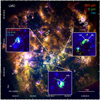 |
Fig. 1 Color-composite image of the LMC combining the Hα (blue, Smith et al. 2000), SAGE/IRAC 8 µm (green, Meixner et al. 2006), and HERITAGE/SPIRE 350 µm (red, Meixner et al. 2013) images. The positions of the 20 ALMA fields are marked with white circles 15 times larger than the field of view of our ALMA observations and the field number. The color-composite images of the fields with hot core detection combining the VMC K-band (blue, Cioni et al. 2011), ALMA CS (5–4) peak intensity (green, this work), and 1.2 mm ALMA continuum (red, this work and Paper II) images are shown as insets. The hot cores reported in this paper, 4A (ST16; Shimonishi et al. 2020), 6A (N105-2 B; Sewiło et al. 2022), 6B (N105-2 A; Sewiło et al. 2022), and 14A are highlighted in the insets images. |
Spectral cube parameters for primary beam corrected images.
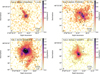 |
Fig. 2 Examples of the 1.2 mm continuum emission toward four regions of the LMC sample. The contours show the three, six, and nine times the σrms. The identified compact cores are highlighted with white contours at 50% of the peak emission. The synthesized beam of the images and a scale bar are shown in the bottom-left and bottom-right corners of each panel, respectively. See Paper II for more details on the 20 fields observed across the LMC (see Table 1). |
3.1 Spectral analysis of the continuum cores
In this section, we present the steps to analyzing the extracted spectra from the 65 compact sources identified in the ALMA 1.2 mm continuum images (see Paper II). The spectra of each source were extracted from the primary beam corrected cube images of the four spectral windows (see Table 2). The average spectra were computed using the spectral-cube python package (Robitaille et al. 2016) with the pixels enclosed within the 50% peak-intensity contour of the 1.2 mm continuum emission maps. Figure 3 shows an example spectrum (see Appendix A for the rest of the spectra).
As a first step in the analysis of the extracted spectra, we identified the molecular lines toward the most chemically rich sources (i.e., spectra with the largest number of line detections; see Fig. 3 for an example) using the CDMS catalog (Cologne Database for Molecular Spectroscopy; Müller et al. 2005). For this, we estimated the noise level (σrms) in each spectrum (i.e., for each source and spectral window) by performing a sigma clipping analysis. Based on this noise-level determination and the intensity of each spectral line feature, we sorted the detected lines. We considered the lines as a definite detection if their peak value exceeded 5σrms and as tentative features if the line strength is between 3 and 5σrms. The definite and tentative detections are respectively labeled with black and gray in Figs. 3 and A.1–A.20. With a complete set of molecules presented in Table 3, including definite and tentative detections, we fit the spectra using the XCLASS toolbox3 (extended CAS A Line Analysis Software Suite; Möller et al. 2017, 2023, with additional extensions, T. Möller, priv. comm.). XCLASS solves the radiative transfer equation in one dimension in local thermody-namic equilibrium (LTE) or non-LTE based on the request. It can solve the radiative transfer equation for an unlimited number of molecules simultaneously, taking line blending into account and producing modeled spectra. XCLASS provides the basis for finding the best-fit model to the observed spectra by encompassing a large set of fitting algorithms available within the MAGIX interface (Möller et al. 2013). The fitting procedure works with the χ2 minimization. The contribution of a certain molecule can be described by more than one component. This is useful when the detected molecular emission line may come from different unresolved structures with different sizes, temperatures, or even distances to the observer. Each component is described by source size, temperature, column density, line width, and velocity offset. These can be fixed or free to vary to get the best-fit spectra and the best set of parameters.
Using XCLASS, we analyzed the spectra assuming that all the considered molecular species are located within a core layer at the position of the source (i.e., we did not consider foreground clouds located between the source and the observer). In the absence of optically thick transitions, column density and source size are degenerate and cannot be determined separately. Therefore, we fixed the source size for all the molecules to a very large value to impose a beam-filling factor of one4. The temperature, column density, line width, and velocity shift are in general free parameters to fit. While parameters such as line width and velocity shift can be determined from Gaussian fits to the detected spectral lines, a good determination of the temperature requires the detection of several transitions from the same molecular species. Based on this, we grouped the molecules into two different categories: molecules with more than two transitions detected within the four spectral windows and molecules with only one or two transitions. The first group includes CH3OH, SO2, and CH3CN, and we fit the temperature for them using XCLASS when multiple transitions were detected.
Out of 65 sources, CH3OH was detected in 48, while 37 sources show clear detections of three or more transitions. One or two transitions were detected toward the other 11 sources. Seventeen sources have no CH3OH features with line intensities higher than 3σrms. In the first iteration, we fit CH3OH using an LTE approximation, which resulted in low temperatures (5–17 K; see Table B.1) and some line features to be underfit or overfit (see Fig. B.1). Based on these inaccuracies, we switched to non-LTE for fitting CH3OH, which resulted in better fits. In the non-LTE description, we have two additional parameters to consider: the ratio of A and E CH3OH and the collision partner5 volume density. We fixed the A to E CH3OH ratio to one and fit the collision partner density in the cores with more than two CH3OH lines. The fit collision partner densities are ≈ 106 cm−3 for most of the cores and about ~107 cm−3 for those cores with bright CH3OH lines. For the sources with one or two CH3OH lines, we fixed the density of collision partners to the median value of the rest of the cores: 2.0 × 106 cm−3. With this, we then fit the temperature, column density, line width, and velocity offset. The derived gas kinetic temperatures for CH3OH with the non-LTE description are generally in the range of 20–60 K (see Table B.2). Finally, for those sources with no CH3OH detection, we fixed the temperature to the median value of the other cores and the line width and velocity offset to values derived for CS, if this was detected, and we derived an upper limit for the CH3OH column density.
We found SO2 to be present in 12 sources with enough lines for temperature determination under LTE conditions. However, only in five sources were there enough SO2 lines to fit the spectra using non-LTE. For these sources, we compared the LTE and non-LTE fits, finding no major differences in the output temperatures and fit quality. Therefore, we fit SO2 for all the fields using an LTE approach. For the rest of the molecular species, we fixed the temperature to the best-fit value for CH3OH. If CH3OH was not detected or properly fit in the spectra of a source, we fixed the temperature of other molecules to the median of the best-fit value for CH3OH from other sources.
For four sources (4A, 6A, 6B, and 14A), a one-component model for CH3OH and SO2 did not give satisfactory results. A two-layered morphology with a hot central component and a colder envelope as the foreground provided the most convincing results. The core component’s source size was fixed to a sub-beam size (not beam filling), while the foreground component was set to fill the beam. In these sources, we detected several transitions of CH3CN with a high enough S/N, which provided an additional temperature estimate. As done for the other sources in the sample, for the rest of the molecules, we fixed the temperature to what was derived from the hot component of CH3OH. Moreover, some isotopologues were also detected in these sources. We used the flexibility of XCLASS to link the isotopologues to the main species, giving them the same temperature and velocity profile to fit the isotopologue ratio from the ratio of column densities. We also detected HNCO and tentatively detected HDCO, HC3N, and NH2CHO in one or more cores among these four cores. Furthermore, we estimated an upper limit for HDCO, NH2CO, CH3CHO, and CH3OCH3 in these four cores when they appeared in the spectra, but they were not fit properly due to having a low S/N (S/N < 3). To this purpose, we fixed the temperature and line width and velocity shift to the hot component of CH3OH. These transitions are marked with red in the figures of the corresponding spectra. In addition, we searched for hydrogen recombination lines (RLs) in all sources. Within the four observed spectral ranges, there are two potentially detectable RLs (H36β and H41γ). However, we only found one tentative detection of H36β toward source 3A (see Fig. A.3). We used XCLASS to fit the RL emission. For the fit, we fixed the electron temperature to 104 K (e.g. Selier & Heydari-Malayeri 2012; Jin et al. 2023) and fit the other three parameters, obtaining an emission measure estimate of 2.5 × 10⁶ pc cm−6, a line width of 18.2 km s−1, and a velocity offset of 284.4 km s−1, consistent with the velocity derived for the molecular species.
The fitting procedure in XCLASS uses an algorithm chain from the MAGIX interface, including the genetic algorithm as a global minimizer and the Levenberg-Marquart algorithm as a local minimizer. We also ran XCLASS with a Markov chain Monte Carlo (MCMC) algorithm on a few spectra to estimate typical errors on the different fitting parameters. The error values range from 40–60% for the temperatures, 20–40% for the column densities, and 10–30% for the line widths and velocity shifts. In the non-LTE solution, there is a degeneracy in defining the temperature, column density, and collision partner density that makes it hard to agree on an error value. The outcome of the fitting procedure is shown as modeled spectra (in black) overlaid on observed spectra (in colors) in Figs. 3 and A.1–A.20. The best-fit parameters are listed in Table B.2, and the upper-limit estimations are marked with a less than (<) sign.
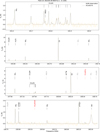 |
Fig. 3 ALMA Band 6 observed spectra toward source 14A overlaid with the best-fit XCLASS model. Molecular transitions with definite detections (S/N > 5) are represented by solid black lines, while those with tentative detections (3 < S/N < 5) are denoted by dotted gray lines. Dotted red lines indicate transitions of molecules for which abundance upper limits are provided. |
Definite and tentative detections of molecular species along with the corresponding number of sources exhibiting these emissions.
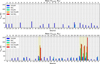 |
Fig. 4 Best-fit XCLASS temperature for different molecular tracers. In case of definite detection in more than two transitions, CH3OH, SO2, and CH3CN were free for fitting (for more details, see Sect. 3.1). There is an uncertainty of 40–60% for the temperatures. The sources are ordered by increasing mass (from Paper II), calculated with the temperature of the CH3OH (cold) component to account for the total mass in the core. The hot cores are highlighted with yellow bars. |
3.2 Results from spectral analysis
3.2.1 Temperature of compact cores
As discussed in Sect. 3.1, we fit the temperature for three molecular tracers, CH3OH, SO2, and CH3CN, when there were firm detections. This resulted in 47 sources with a temperature determination using CH3OH, 12 sources with SO2, and only four sources with CH3CN-derived temperatures. Figure 4 shows the derived temperatures for the different molecular tracers for all 65 compact cores. The cores are ordered based on their mass (as determined in Paper II).
As stated earlier, out of the 65 cores, only four have a reliable temperature determined using CH3CN, and it is only for these four cores that we needed more than one component to fit SO2 and CH3OH (see Table B.2). Furthermore, we only obtained temperatures above 100 K for the hottest component of these four sources, with the temperature remaining consistently below 60 K for the rest of the sources. Based on the definition of a hot molecular core to have a temperature higher than 100 K, we can classify these four sources (4A, 6A, 6B, and 14A) as such. These hot cores are likely embedded in a colder envelope with temperatures about 30–40 K, similar to the temperatures derived for the other cores in the sample.
3.2.2 Line-width of different molecules
The line width of a molecular species provides useful information about the kinematics of the gas. Figure 5 compares the line widths derived for different molecular species from fitting the Gaussian line profile with XCLASS (see Sect. 3.1). Six molecules, including the ubiquitous ones, CS, SO, CH3OH, and two other abundant species, SO2 and H13CO+, together with the shock tracer SiO were utilized. The line widths vary between 1 and 35 km s−1, with methanol having the lowest value in 49% of the cores. In this plot, we present the line width value for the hot component of SO2 and CH3OH when there are two temperature components. A value of 5 km s−1 is shown with a dashed line as a reference. The number of cores with line-width values larger than 5 km s−1 for at least one of the molecular species is 16. In nine of these sources, SiO is one of the molecules with a large line width suggesting the presence of molecular outflows, which will be studied in a forthcoming paper. Among them, we can identify the four cores (4A, 6A, 6B, and 14A) with temperatures higher than 100 K (see Sect. 3.2.1 and Fig. 4).
3.2.3 Chemical contents of the cores
Several molecular lines were detected in the spectra of each core. Among all the species, methanol was detected toward 74% of the cores (48/65). Among 17 cores with no-CH3OH line detection, seven cores showed no emission lines at all (8B, 11A, 13B, 14B, 16A, 17B, and 19B). Other molecular species with high detection rates include CS, SO, SO2, H13CO+, H13CN, HC15N, H2CS, and SiO, while more complex molecules, such as HDCO, HNCO, HC3N, and CH3CN or isotopologues of SO and SO2, were detected only toward a small subset of objects (about 8% of the sample). We also report a tentative detection of NH2CHO in one of the cores (6A). Moreover, CH3OCHO or CH3OCH3 emerged in the modeled spectra after fitting an upper limit column density for them toward the cores 4A, 6B, and 14A. In addition, a hydrogen RL, H36β, was detected tentatively toward the most massive core in our sample (3A). In addition, H41γ is also in the observed bands, and we mark it with red on the spectra of this core, as it was detected with an S/N less than three. The detection of this RL suggests the presence of HII regions that likely contribute to the 1.2 mm continuum emission. Preliminary data at 6 GHz obtained with ATCA (Hamedani Golshan, priv. comm.) favors this interpretation. The mass derived for this source is likely overestimated in the current analysis. Interestingly, we have a tentative detection of CH3CN towards the source 3A. The detection of CH3CN, which is only clearly detected toward the four cores 4A, 6A, 6B, and 14A in the sample (see Sect. 4), together with the detection of RLs (likely related to an HII region) in 3A suggests the presence of a hot core near an expanding HII region, a scenario that is commonly found in several hot cores of the MW (e.g., Kurtz et al. 2000; Sánchez-Monge et al. 2013a; Cesaroni et al. 2017).
We compared the abundances of different molecules in all the sources. The abundances were derived by dividing the column density of every molecule by the molecular hydrogen column density (N(H2), derived in Paper II). For this purpose, we assumed that the dust and gas at the position of the source are well mixed and have the same temperature as derived from the XCLASS fits (see Table B.2). Figure 6 shows the abundance of the molecules with the highest detection rate for all the cores, whereas in Figs. 7–10, the molecules are grouped into three different groups: S-bearing species (SO, SO2) and SiO; N-bearing species (H13CN, HC15N, and HNCO) and (HC3N, CH3CN, and NH2CHO); and O-bearing species (HDCO, CH3OCHO, CH3OCH3). We ordered the cores based on their mass, but we did not see any clear correlation between mass and abundance for any of the species. When comparing the different groups of molecules, we observed that S-bearing species are, on average, more abundant than N- and O-bearing species.
Finally, comparing all the abundance plots, it was evident that four sources show a rich chemistry with the presence of various molecular species. These sources would classify as hot molecular cores based on their chemistry, as well as their temperatures, since these objects are the only cores with temperatures above 100 K and average line widths above 5 km s−1. Interestingly, these four sources are those with the largest SO2 abundances, thus supporting the interpretation by Shimonishi et al. (2023) that bright SO2 lines are a good tracer of hot molecular cores in the low-metallicity environment of the LMC and SMC.
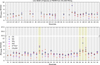 |
Fig. 5 Best-fit XCLASS line width (full width at half maximum, FWHM) for different molecular species. The line width of 5 km s−1 is marked with a dashed line as a reference. There is an uncertainty of 10–30% for the line widths. The sources are ordered by increasing mass (from Paper II) with the temperature of CH3OH (cold) component to account for the whole mass in the core. The hot cores are highlighted with yellow bars. |
4 Discussion
4.1 Hot cores in our survey
Based on the spectral analysis of the 65 continuum sources, we report the detection of four hot molecular cores and one hot core candidate from the ALMA observations of 20 fields hosting YSOs in the LMC. As highlighted in Sect. 3, four cores (4A, 6A, 6B, and 14A) have temperatures above 100 K, large line widths, and the highest chemical richness among all the cores in the sample. This, together with the fact that the spatial size of these cores where the emission reaches half of the peak value in the continuum map, Ωobs (Ωdeconv), is between 0.12 (0.08) and 0.14 (0.11) pc (see Paper II) suggest that they are in the hot molecular core phase. This result confirms the previous detection of hot cores in ST16 YSO (Shimonishi et al. 2020) and two hot cores N105-2 A and N105-2 B in the N105 star-forming region (Sewiło et al. 2022). In addition, we present a new hot core detection in field 14: 0523333.40–693712.1, 14A. With this new detection, the number of known hot cores in the LMC increases to seven.
Isotopologues of SO and SO2 were detected toward the hot cores in our sample. The hot cores 4A and 6A show emission lines3f4rom 33SO, 33SO2, and 34SO2. Hot core 6B contains 33SO and 34SO2 but no 33SO2, and the core 14A shows no reliable detection of these isotopologues. We derived the isotopic ratios of 32S/33S and 32S/34S toward hot cores 4A and 6A and found them to vary between 12 and 21 and 9 and 19. These values can be compared with previous estimates in the LMC and other galaxies. Gong et al. (2023) used the APEX 12-m telescope to measure sulfur isotopic ratios in the LMC and compiled a set of measurements toward the LMC, different regions of the MW, and starburst galaxies (see their Table 2). For the LMC, Gong et al. (2023) found the ratios of 32SO/33SO and 32SO/34SO to range between 27 and 53 and 15 and 19, respectively. Combined with our results, which are similar to or slightly lower than previous estimates, the range for these isotopic ratios increases to 12–53 for 32SO/33SO and 9–19 for 32SO/34SO. The sulfur isotopic ratios in the LMC are lower than in different regions throughout the MW but more consistent with measurements in starburst galaxies. Gong et al. (2023) suggest that the low values in the LMC might be attributed to a combination of age, low metallicity, and star-formation history.
Source 3A may be a potential hot core candidate based on the presence of COMs in the analyzed spectra. This source is associated with a common hot core tracer, CH3CN. However, the temperatures that we derived for this source are below 100 K. We note that source 3A is also associated with RLs in addition to CH3CN, suggesting a scenario where a compact hot core may be located in the near vicinity of an HII region. Future observations of these objects at higher resolution as well as covering additional frequency ranges may help in unambiguously determining the presence of hot cores in this region.
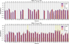 |
Fig. 6 Abundances of molecular species with a high detection rate in our sample. There is an uncertainty of 20–40% on the column densities. The sources are ordered by increasing mass (from Paper II) with the temperature of CH3OH (cold) component to account for the whole mass in the core. The hot cores are highlighted with yellow bars. The arrows show an upper-limit estimation. |
4.1.1 New hot core in the LMC
The newly identified hot core 14A is located at the position of the YSO 0523333.40–693712.1. The color composite image from the 1.2 mm continuum (dust emission, in red), CS (dense gas tracer, in green), and K-band (tracer of stellar population and possible H2 emission, in blue) in the lower insert panel of Fig. 1 shows the peak emission toward the position of the hot core. Figure 11 shows the integrated intensity maps of different molecular species toward the hot core 14A, with the 1.2 mm continuum emission shown in contours as reference. Apart from the bright emission toward the hot core position, the CS map also reveals prominent filamentary structures. The emission from CH3OH, SO, H13CO+, and H2CS show faint elongation in the north-south direction. Moreover, HNCO and HDCO show a very faint emission, offset from the hot core, and H2CS emission also peaks offset to the hot core, where the HNCO emission peaks.
4.1.2 Comparison of hot cores common to other studies
In addition to 14A, which is detected for the first time in this work, the other three hot cores (4A, 6A, and 6B) have previously been identified in other studies based on independent observational datasets. In the following, we compare our results with those in the literature for the temperatures and abundances of species detected toward all the cores, including CH3OH, CH3CN, HNCO, H13CO+, SO2, SO, and SiO.
Shimonishi et al. (2020) reported the detection of a hot molecular core based on ALMA Band 6 and 7 observations of the embedded high-mass infrared source ST16. Our study results in the detection of the same hot core that we name 4A following the adopted nomenclature. The hot components of CH3OH and SO2 have the same temperatures in both studies considering uncertainties (see Fig. 12, top-left panel). However, the cold component of both species has slightly lower temperatures in our study, and the derived temperature from CH3CN is larger by a factor of 1.5. The top-right panel of Fig. 12 compares the abundances from the two studies, after accounting for the difference in the gas-to-dust mass ratio assumed in our study and that of Shimonishi et al. (2020)6. While the abundances for SO2, and SiO are slightly higher in the current work, CH3OH, CH3CN and SO show lower abundances. The higher temperature and lower abundance for CH3CN in the current work could be due to a possible degeneracy between these two parameters when fitting the spectral data, suggesting that these two sets of parameters can reproduce the observed lines. Further observations can help in better constraining both the temperature and density for this hot core. Sewiło et al. (2022) found two hot cores, N105-2 A and N105-2 B, from Cycle 7 Band 6 observations of three fields in the N105 star-forming region. We note that the hot cores 6B and 6A in the current study correspond to the objects N105-2 A and N105-2 B, respectively. The temperature estimations are in good agreement for each pair of sources (see Fig. 12, middle-and bottom-left panels), with larger variations happening for the cold components of CH3OH and SO2 in 6B compared to N105-2 A. The middle- and bottom-right panels of Fig. 12 compare the abundances from the two studies. Sewiło et al. (2022) assumed a gas-to-dust mass ratio of 316, very close to the value we use, 320. The abundances of nearly all the molecules in 6A compared to N105-2B fall in the same range except CH3OH and CH3CN, which are slightly higher in N105-2B. Similar results were obtained for 6B and N105-2 A, with abundances falling in the same range. However CH3OH, HNCO and H13CO+ show abundances approximately two to five times lower in 6B (this work). The observed differences are likely due to the slightly different temperatures used to calculate the column densities in both studies. Finally, we searched for detections of other species, such as HDCO, CH2CO, and NH2CHO, that had been previously detected by Sewiło et al. (2022). We could not confirm their detection because the expected brightness of the species is less than the sensitivity of the current dataset. Only a tentative feature was seen for NH2CHO toward source 6A (see Fig. A.6).
Overall, the differences in the molecular abundances between the different works are within a factor of less than five. This factor is acceptable considering all possible errors and uncertainties in the analysis process. For example, different inter-ferometric filtering during the observations as well as weather conditions or calibration effects, procedures followed to extract the spectra, or methodology used for fitting the lines may affect the derived temperatures and abundances by factors commonly in the range of two to ten. Therefore, we consider that our derived abundances are in agreement with previous studies, and we used them in the following discussion.
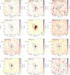 |
Fig. 11 Peak-intensity images of the molecular species detected toward hot core 14A. The maps are ordered based on the frequency of the transition from left to right, top to bottom. The 1.2 mm continuum contours with contour levels of three, six, and nine times the σrms and the 50% 1.2 mm continuum contour are overlaid in each image for reference. Top is north and right is west. |
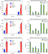 |
Fig. 12 Comparisons of the derived temperatures (left) and abundances (right) from the current study and the literature. The top panels show a comparison of 4A and ST16 (Shimonishi et al. 2020), the middle panels show 6A and N105-2B, and the bottom panels show 6B and N105-2A (Sewiło et al. 2022). An error range of 40% is depicted for the temperatures and column densities from the current paper. |
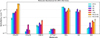 |
Fig. 13 Abundances of different molecular species for all the known hot cores in the LMC after scaling to the gas-to-dust mass ratio. The LMC hot cores are ST11 (Shimonishi et al. 2016a), 4A, 6A, 6B and 14A (this work), and N113 Al and N113 B (Sewiło et al. 2022). Black arrows show an upper limit estimation. An error range of 40% is shown on the abundances from the current paper. |
4.2 Properties of hot cores in the LMC
4.2.1 Comparison of the hot cores in the LMC
Apart from the four hot cores discussed in the previous section, three more have been reported in the LMC. Sewiło et al. (2018) discovered the first two chemically rich hot cores in the N113 star-forming region, N113A1 and N113 B3, with COMs with up to nine atoms being detected in extra-galactic hot cores for the first time. The abundance of the molecular species for these objects, after scaling for metallicity, falls on the lower end of the Galactic values. In contrast, the hot core ST 11 reported by Shimonishi et al. (2016b) was detected based on the presence of hot SO2, although no reliable COMs were detected. The absence of COMs in this hot core was explained by a hot dust temperature resulting in inefficient CO hydrogenation to form CH3OH (Shimonishi et al. 2016b).
Figure 13 shows a comparison of the molecular abundances in the seven hot molecular cores detected to date in the LMC after scaling to the gas-to-dust mass ratio used in the current paper (see Sect. 4.1.2). Each bar stands for one hot core, with error bars and upper limits also depicted in the plot. The non-detections of CH3CN, HNCO, H13CO+, and SO toward N113 A and N113 B are due to a lack of bright transitions of these species in the observational setup, whereas the upper limits for ST11 show the absence or underabundance of this species, which was in the observed frequency ranges but not detected. The methanol abundance varies between 3.6 × 10⁻⁹ for 4A and 6A and 5.3 × 10⁻⁸ for N113 Al, where it is detected. The abundance of SO2 varies between 5.0 × 10⁻⁹ for 6B and 2.1 × 10⁻⁸ for 4A and ST11.
The abundances shown in Fig. 13 reveal some trends for the hot cores in the LMC. We found an ascending pattern of an order of magnitude in the abundance of CH3OH from the ST 11 to N113 region, while the abundance of SO2 shows small variations among the hot cores. At a second level, there seems to exist a correlation between CH3OH and SiO. If SiO is produced in shocks, likely associated with molecular outflows (e.g. Schilke et al. 1997; Sánchez-Monge et al. 2013b), this correlation may suggest that the higher abundance of CH3OH for some sources may have a shock origin. These correlations will be explored in a forthcoming work evaluating the spatial correlation of multiple molecular species.
4.2.2 Comparison with chemical models
The presence of hot SO2 in ST11 has been taken as a signature of a hot core, with the absence of COMs in this source strengthening the idea of a warm dust chemistry in the LMC (see e.g. Shimonishi et al. 2016b). Although only one hot core of this kind has been detected in the LMC, we took advantage of the hot core models by Acharyya & Herbst (2018) to investigate how the warm dust hypothesis for low-metallicity environments compares to the current observations of hot cores in the LMC.
Acharyya & Herbst (2018) simulated the stages of star formation leading to hot cores and their lower-mass counterparts, hot corinos, under the conditions of the LMC (and the SMC). They used a gas-to-dust mass ratio of 175, a cosmic-ray ionization rate of 1.3 × 10⁻¹⁷ s−1, and a radiation field strength similar to the Galactic values. The star formation was modeled in three stages. The first stage is an isothermal cloud collapse under free fall with fixed gas and dust temperatures of 10, 15, 20, and 25 K and a visual extinction Av of 1.64 mag. The collapse is stopped when the density reaches 107 cm−3, a process that lasts 9.3 × 10⁵ yr, during which Av increases up to ≈450 mag. In the second stage, the density is fixed at 107 cm−3, while the temperature increases linearly with time up to 100 or 200 K, resembling the temperature of hot cores. Two different times for the heating process are considered, reproducing expected conditions for high-mass (5 × 10⁴ yr) and low-mass (106 yr) star formation. Once 100 or 200 K is reached, the warm-up ceases, and the newly formed hot core is allowed to evolve until a final total time of 107 yr. This model does not include the effects of shocks in the chemical evolution.
Figure 14 shows the time evolution of SO2, CH3OH, and CH3CN abundances for the hot core model described above for the 100 and 200 K final temperatures (for other molecules see Figs. C.1 and C.2). The observed abundances for the seven hot cores in the LMC are overlaid as horizontal lines in each panel following the same color scheme as in Fig. 14. Interestingly, only the models where the initial dust temperature is assumed to be between 10 and 20 K reproduce the observed molecular abundances. The chemical model with an initial highest dust temperature of 25 K results in molecular abundances that are much lower than the observed ones. Based on the comparison with the chemical models of Acharyya & Herbst (2018), a high initial dust temperature does not seem to be a reason for a possible lack of COMs in the hot cores of the LMC since chemical models with initial dust temperatures in the range 10–20 K (similar to star-forming regions in the MW) can better reproduce the molecular abundances observed in the LMC.
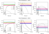 |
Fig. 14 Comparisons of abundances for SO2, CH3OH, and CH3CN from observations of the seven hot cores detected in this galaxy and the LMC hot core models for the final hot core temperature of 100 K (top) and 200 K (bottom). The black curves show abundances over time for an initial dust temperature of 10 (dotted curve), 15 (dashed curve), 20 (larger dashed curve), and 25 K (the solid curve). The horizontal colored line shows the single abundance value for each hot core and follows the same color code as Fig. 13 (see the text for more details). |
4.3 Hot cores in the LMC, SMC, and MW
A logical next step when studying the chemistry in low-metallicity environments is to compare the molecular abundances from the hot cores in the LMC, SMC, and outer Galaxy to those found in star-forming regions in the inner Galaxy. To achieve this goal, we collected a sample of Galactic hot cores studied in the literature and added them to the seven hot cores found in the LMC (see Sect. 4.2), the two hot cores recently discovered in the SMC (Shimonishi et al. 2023), and the WB 89–789 SMM1 hot core found in the outer regions of the Galaxy (Shimonishi et al. 2021). In the case of WB 89–789 SMM1, we used the abundances calculated for a source with a size of 0.1 pc (from Table 4 of Shimonishi et al. 2021). In the interest of matching spatial scales, we focused on single-dish observations of Galactic hot cores. In particular, we considered the Orion Hot Core (Sutton et al. 1995), Sgr B2(N) (Nummelin et al. 2000) and W3(H2O) (Helmich & van Dishoeck 1997) to represent the standard conditions and properties of hot cores in the MW.
In Fig. 15, we present a comparison of the abundances of four molecular species corresponding to the selected list of hot cores. For the LMC hot cores, we first applied a correction factor to account for the different gas-to-dust mass ratio every study assumes (see Sect. 4.1.2). Then we applied a correction factor of 5, 2.6, and 4 to the abundances of the hot cores in the SMC, LMC, and extreme outer Galaxy7 to account for differences in metallicity. The original values are shown with single color bars in Fig. 15, while the scaled values are depicted as an excess with dotted patterns.
The methanol abundances vary by an order of magnitude among the hot cores in the LMC, except for ST11, for which only an upper limit is estimated. While the methanol abundances show an ascending trend from the low metallicity of the SMC to the LMC and to the inner regions of the MW, the only hot core in the outer region of the Galaxy, with a factor of four lower metallicity, shows the highest methanol abundance. We note that CH3CN was not detected in all the hot cores, making the comparison less robust. However, one can see that the abundance of CH3CN in the hot core in the outskirts of the Galaxy is higher than those in the LMC. In contrast to higher abundances of CH3OH and CH3CN in the outer Galaxy compared to the LMC and SMC, SO2 and SiO are less abundant. This raises the question of whether the abundance of different molecular species is only a function of metallicity. We note that the outskirts of the Galaxy are more quiescent due to the low star-formation activity, while the star-forming regions of the LMC and the SMC are more active. While comparisons of the chemistry in different conditions still need better observational statistics, we acknowledge the necessity of chemical modeling to further investigate the effect of metallicity, strength of UV radiation, cosmic ionization rate, and shock chemistry on the observed molecular abundances.
Shimonishi et al. (2020) classified the LMC hot cores as “organic-poor” and “organic-rich” based on the comparison of only four hot cores in the LMC. Sewiło et al. (2022) placed N105-2 A and N105-2 B in the organic-rich class, suggesting a larger sample to verify this classification. We also acknowledge the necessity of larger samples for a better understanding of hot core chemistry in the LMC. At the same time, we revise the classification of organic-poor and organic-rich based on the findings of this study. Shimonishi et al. (2020) classified ST11 and ST16 as organic-poor and N113 Al and N113 B3 as organic-rich hot cores to emphasize the detection of more complex compounds with comparable scaled abundances to the Galactic hot cores. Our survey study, however, demonstrates a different picture. All the hot cores in our sample show comparable chemical complexity. A slightly different chemistry may relate to the evolutionary stage of the hot core and surrounding gas. For example, we detected isotopologues of SO2,33SO2, and 34SO2 in the hot core 4A but had no detection of deuterated molecules. In contrast, hot core 14A shows emission lines from HDCO but no emission from SO2 isotopologues. The common association of deuterated species with early evolutionary stages (e.g. Fontani et al. 2011; Treviño-Morales et al. 2014) and the connection of SO2 with the presence of shocks and ionized gas (e.g. Minh et al. 2016; Gieser et al. 2021) suggest that different evolutionary stages and physical conditions are likely relevant factors of the chemical content of the hot cores in the LMC. Within this picture from the hot cores in the LMC, the only organic-poor hot core that remains is ST11.
In Fig. 16, we present pair-wise comparisons of the abundances of CH3CN, CH3OH, SO2, SO, and SiO. Based on these comparisons, we observed that the hot cores in the LMC appear to show lower abundances of CH3CN relative to CH3OH compared to hot cores in the MW but higher abundances of SO2 relative to SO. Although this study should be extended to a larger sample of targets and evolutionary effects may play a role in the observed abundances, the first results favor the idea that hot cores in the LMC may be brighter in SO2 lines compared to other molecular species commonly found in hot cores. The comparison and correlation between CH3OH and SO2 with SiO suggest that shocks may play an important role in the observed abundances of these species.
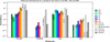 |
Fig. 15 Abundances of CH3OH, CH3CN, SO2, and SiO for all known hot cores in the SMC and LMC and for a selection of Galactic hot cores. The SMC hot cores are included, SO7 and SO9 (Shimonishi et al. 2023). The LMC hot cores are ST11 (Shimonishi et al. 2016a), 4A, 6A, 6B and 14A (this work), and N113 Al and N113 B (Sewiło et al. 2022). We selected four Galactic hot cores: an outer Galaxy hot core (Shimonishi et al. 2020), Orion Hot Core (HC) (Sutton et al. 1995), Sgr B2(N) (Nummelin et al. 2000), and W3(H2O) (Helmich & van Dishoeck 1997). The extent of each bar with a dotted pattern represents the abundances scaled to the Galactic metallicity. |
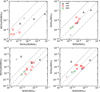 |
Fig. 16 Comparisons of the abundances of CH3OH and CH3CN and SO2 and SO for the hot cores in the SMC (open green circles), LMC (red rectangles), and MW (black triangles for inner Galactic hot cores and gray triangle for outer Galactic hot core). Dashed lines show abundance relations of 1:1 for the top-right panel and 1:100 for the other panels. The dotted lines show a variation of a factor of ten above and below the relations described by the dashed lines. |
4.4 Location of hot cores in the LMC
In Fig. 17, we show the location of all the detected hot cores in the LMC. So far, all the hot cores associated with COMs are located in the central region of the galaxy, which is known as the LMC bar. This region has a mildly higher (~2%) metallicity compared to the surrounding regions, as suggested by narrowband near-IR observations (Choudhury et al. 2021). Inspection of the atomic(Kim et al. 1998; Smith et al. 2000), molecular gas (e.g. Fukui et al. 1999), and dust maps (Meixner et al. 2013) of the LMC revealed that the dense cold gas and dust are located within a zigzag shape in the bar region and surrounded by bubbles of dispersed dust and gas (known as HI holes; Staveley-Smith et al. 2003). This implies that expanding material from different sides results in compressed material into this zigzag region. Based on this observational evidence, we speculate that star formation in the bar must have been triggered at some point when the interstellar medium in the bar was enriched and the metallicity was increased relative to other areas of the LMC. This might explain the preferential detection of hot cores with complex chemistry only toward the LMC bar.
For this scenario to be plausible, one needs to consider if the ignition of the new generation of stars that resulted in the currently detected hot cores took place after the chemical enrichment of the interstellar medium of the LMC bar. Different works in the literature explore the origin of the current distribution of gas and dust in the bar region as well as the existence of possible events in the history of the LMC that may have caused an increase of metallicity in the bar and the triggering of a new generation of stars. In the following, we summarize the main findings and connect them to the presence of hot cores in the LMC bar.
Hydrodynamic simulations (Tenorio-Tagle et al. 1986) infer the creation of Hi holes and shells as a result of the interaction between high-velocity clouds and the galactic disk. At the same time, the study of the morphology and kinematics of stellar populations and HI gas in the LMC, SMC, Magellanic Bridge (MB), and the Leading Arm (LA) suggests the interaction between the LMC and SMC (e.g. Zivick et al. 2019, and references therein). Furthermore, numerical simulations of the evolution of the Magellanic Clouds favor the sporadic replenishment of low-metallicity gas from the SMC to the LMC’s disk over the last 2 Gyr as a result of their tidal interaction (known as Magellanic Squall; Bekki & Chiba 2007). This stripped high-velocity gas can be responsible for some of the HI holes observable in the LMC. Bekki & Chiba (2007) argues that the triggering of the star formation could be a direct impact of clouds of the SMC interacting with those of the LMC. In addition, numerical models of Besla et al. (2012) investigate the history of interaction between the SMC, LMC, and MW. Besla et al. (2012) argue that the off-center warped stellar bar of the LMC and its one-armed spiral can be explained by a recent direct collision with the SMC.
Given the uncertainties of the model parameters, the exact time of the collision and its impact on star formation cannot be strictly defined. However, a time range from 100 to 300 Myr seems a reasonable approximation (Besla et al. 2012). Analysis of the proper motions of stars from Gaia data supports the direct collision and suggests that this event was not a grazing interaction but that the SMC went directly through the LMC, allowing the interstellar medium of both galaxies to interact (Zivick et al. 2019). Furthermore, Choudhury et al. (2021) presumed that the mixing of the metallicity of the two galaxies, caused by tidal interaction, could be a reason for the asymmetry metallicity distribution observed in the LMC. With all this, and given the timescale of formation of hot molecular cores (~105 yr, Wilner et al. 2001; Furuya et al. 2005; Herbst & van Dishoeck 2009), the detected hot cores in the LMC bar region have most likely been formed in the inhomoge-neous and slightly metallicity-richer interstellar gas that emerged after the severe interactions of the LMC and the SMC.
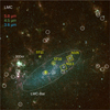 |
Fig. 17 Three color composite image of the LMC combining 3.6 (blue), 4.5 (green), and 5.8 µm (red Meixner et al. 2006) images to highlight the position of the stellar bar. The dashed ellipse marks the bar region. The 20 ALMA fields from the current study are overlaid with white circles 15 times larger than the field of view of our ALMA observations. The fields accommodating hot cores are highlighted in yellow, including the YSO ST16 and N105 star-forming region. The field marked with a star shows the position of the new hot core detected in our survey. The location of the hot cores in N105 (Sewiło et al. 2022) and N113 (Sewiło et al. 2018) are marked with yellow rectangles. The hot cores ST11 (Shimonishi et al. 2016b) and ST16 (Shimonishi et al. 2020) are shown with yellow plus signs. The hot core ST11 with no COMs is the only hot core detected out of the LMC bar. |
5 Conclusions
We have observed 20 star-forming sites distributed throughout the LMC with ALMA in four frequency ranges between 241 and 260 GHz and at an angular resolution of ≈0″.35 (corresponding to 0.08 pc). We detected a total of 65 continuum cores whose physical properties (e.g., mass, density, size) are presented in Paper II. In this work, we have studied the chemical content of these compact cores. The main findings are summarized as follows:
The extracted spectra at the location of the cores show different levels of chemical complexity in the cores. There are cores with no molecular line emission and cores with single-line detection of dense or warm gas tracers, such as CS, SO, or H13CO+. These include 28% of all the cores. In addition, other cores contain CH3OH. These cores can be put into two distinct groups: cores with emission lines from simple molecules, such as SO2,H2CS, H13CN, HC15N, and SiO, and sources with detection of simple species and COMs, such as CH3CN, or tentative detection of NH2CHO, CH3OCHO, and CH3OCH3.
The detection of multiple transitions from a single molecule allowed for the determination of the temperature. The CH3OH molecule, detected in 72% of the cores, is our main temperature tracer in this study. We estimated the temperature with both LTE and non-LTE assumptions and compared the two temperatures with the SO2 temperature, where it was reliably detected. Our temperature determination was further confirmed by estimating the CH3CN temperature where it was detected.
Molecular line width is a tracer of the gas kinematics. We investigated the line width of different molecular species (fit with XCLASS), and CH3OH showed the lowest line width value in 51% of the cores. However, only a small sample of cores showed an average line width above 5 km s−1.
Comparing the abundance of different molecular species in the 65 cores showed that S-bearing molecules are in general more present and abundant than N- and O-bearing species. Therefore, the detection of N- and O-bearing species, especially the COMs, needs higher sensitivity in future observations.
Four hot molecular cores were detected in this study, confirmed by their size (~0.1 pc), chemical richness, temperatures above 100 K, and high abundances of CH3OH and SO2.
The four hot cores in our sample reveal the detection of one new hot core, bringing the number of hot cores in the LMC to seven. Shimonishi et al. (2023) suggest SO2 as a tracer of hot cores in a low-metallicity environment. Our survey study supports this suggestion by detecting strong lines of SO2 and its isotopologues only in the hot cores. We note that (six out of the seven) hot cores with detections of methanol or other COMs are preferentially located in the LMC bar. The metallicity-scaled abundances of different molecular species in these hot cores are comparable with those in the MW. Shimonishi et al. (2020) have suggested the initial high dust temperature to be responsible for the lower abundances of COMs in the low metallicity of the LMC. However, comparisons of our observed abundances with the LMC hot core chemical models of Acharyya & Herbst (2018) do not support high initial dust temperatures.
Acknowledgements
This paper makes use of the following ALMA data: ADS/JAO.ALMA#2017.1.00696.S. ALMA is a partnership of ESO (representing its member states), NSF (USA) and NINS (Japan), together with NRC (Canada), NSTC and ASIAA (Taiwan), and KASI (Republic of Korea), in cooperation with the Republic of Chile. The Joint ALMA Observatory is operated by ESO, AUI/NRAO and NAOJ. R.H.G. acknowledges the German Deutsche Forschungsgemeinschaft (DFG, German Research Foundation) for supporting this research through project SCHI561/1-1. A.S.-M. acknowledges support from the RyC2021-032892-I grant funded by MCIN/AEI/10.13039/501100011033 and by the European Union ‘Next GenerationEU’/PRTR, as well as the program Unidad de Excelencia María de Maeztu CEX2020-001058-M, and support from the PID2020-117710GB-I00 (MCI-AEI-FEDER, UE). The material is based upon work supported by NASA under award number 80GSFC21M0002 (M.S.). G.A.F. gratefully acknowledges the Collaborative Research Center 1601 (SFB 1601 sub-project A1) funded by the DFG - 500700252. The authors acknowledge the comments provided by the anonymous referee which helped to improve the manuscript.
Appendix A Spectra and XCLASS fits for 1.2 mm continuum cores
Figures A.1 to A.20 show the ALMA Band 6 spectra observed toward the all cores with identified molecular lines (except the core 14B) in the 20 fields observed throughout the LMC. The observed spectra with line detections were fit using the XCLASS software (see Section 3.1), and the results are shown as a black solid line on top of the observed spectra. The molecular species detected in the spectra are marked in black, while the tentative detections are marked in gray.
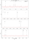 |
Fig. A.1 ALMA Band 6 observed spectra toward source 1A overlaid with the best-fit XCLASS model. Molecular transitions with definite detections (S/N > 5) are represented by solid black lines, while those with tentative detections (3 < S/N < 5) are denoted by dotted gray lines. Dotted red lines indicate transitions of molecules for which abundance upper limits are provided. (See Section 3.1 for more details.) |
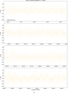 |
Fig. A.14 ALMA Band 6 observed spectra toward source 14B with no emission line detections. (See Section 3.1 for more details.) |
Appendix B XCLASS fits parameters
In Table B.1, we list the parameters assuming LTE conditions for the CH3OH, and Table B.2 collects the fit parameters for CH3OH in non-LTE. We used the non-LTE temperature for methanol to fit other molecules. Therefore, the fit parameters for other molecules are only presented in Table B.2. (For more details, see Section 3.1.) Figure B.1 compares the LTE and non-LTE fit for two methanol lines at 241.767 and 241.792 for two sources, 2C and 14A. While methanol is fit with one component in 2C, 14A gets the best-fitting results with two components for methanol, where the cold foreground component (the envelope) is assumed to be in non-LTE.
Parameters of the LTE fits for CH3OH.
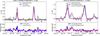 |
Fig. B.1 Comparisons of the LTE and non-LTE fit for two CH3OH lines at 241.767 and 241.791 GHz. |
Parameters of the best-fit model for all detected molecules and their abundances.
Appendix C Comparisons of molecular abundances in hot cores with chemical models
Section 4.2.2 discusses how the observed abundances of the hot cores in the LMC compare with the only hot core modeling for LMC’s condition (Acharyya & Herbst 2018). We present the comparisons for three molecules (CH3OH, SO2, and CH3CN) in Section 4.2.2, and we expand this comparison in this appendix. Figures C.1 and C.2 show the comparisons of observed abundance for the seven hot cores in the LMC with the chemical models for the final hot core temperature of 100 and 200 K, respectively. It is evident from the plots that the solid curve representing the warm dust initial condition (Td = 25 K) does not appear in any of the subplots. The only exception is SiO, for which a sharp increase in the model at a time of ≈106 yr could also reproduce the observed abundances. As the modelings do not include shocks, this increase in the SiO is not reliable. Moreover, the observed abundance of HNCO could not be reproduced by models; the peak abundance of the models is smaller by more than an order of magnitude. The underestimation of abundances is also apparent in the case of SO2 and SO. These three species (HNCO, SO2, and SO) are also commonly found to be associated with shocks in star-forming regions. The higher observed abundances could imply the presence of shocks in the hot cores of the LMC, which is not included in the modelings.
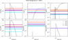 |
Fig. C.1 Comparisons of abundances for CS, SO, SiO, H2CS, HNCO, and NH2CHO from observations of the seven hot cores detected in the LMC and the LMC hot core models for the final hot core temperature of 100 K. The black curves show abundances over time for initial dust temperatures of 10 (dotted line), 15 (dashed curve), 20 (larger dashed curve), and 25 K (solid curve; this curve does not necessarily appear in the range of abundances in the plot). The horizontal colored line shows the single abundance value for each hot core and follows the same color code as Fig. 13 (see the text for more details). |
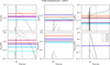 |
Fig. C.2 Same as Fig. C.1 but for the LMC hot core models for the final hot core temperature of 200 K. |
References
- Acharyya, K., & Herbst, E. 2018, ApJ, 859, 51 [NASA ADS] [CrossRef] [Google Scholar]
- Arellano-Cordova, K. Z., Esteban, C., García-Rojas, J., & Méndez-Delgado, J. E. 2021, MNRAS, 502, 225 [CrossRef] [Google Scholar]
- Bekki, K., & Chiba, M. 2007, MNRAS, 381, L16 [Google Scholar]
- Belloche, A., Müller, H. S. P., Menten, K. M., Schilke, P., & Comito, C. 2013, A&A, 559, A47 [NASA ADS] [CrossRef] [EDP Sciences] [Google Scholar]
- Besla, G., Kallivayalil, N., Hernquist, L., et al. 2012, MNRAS, 421, 2109 [Google Scholar]
- Cesaroni, R., Sánchez-Monge, Á., Beltrán, M. T., et al. 2017, A&A, 602, A59 [NASA ADS] [CrossRef] [EDP Sciences] [Google Scholar]
- Choudhury, S., Subramaniam, A., Cole, A. A., & Sohn, Y. J. 2018, MNRAS, 475, 4279 [NASA ADS] [CrossRef] [Google Scholar]
- Choudhury, S., de Grijs, R., Bekki, K., et al. 2021, MNRAS, 507, 4752 [CrossRef] [Google Scholar]
- Cioni, M. R. L., Clementini, G., Girardi, L., et al. 2011, A&A, 527, A116 [CrossRef] [EDP Sciences] [Google Scholar]
- Fontani, F., Palau, A., Caselli, P., et al. 2011, A&A, 529, L7 [NASA ADS] [CrossRef] [EDP Sciences] [Google Scholar]
- Fontani, F., Colzi, L., Bizzocchi, L., et al. 2022, A&A, 660, A76 [NASA ADS] [CrossRef] [EDP Sciences] [Google Scholar]
- Fukui, Y., Abe, R., Hara, A., et al. 1999, IAU Symp., 190, 61 [NASA ADS] [Google Scholar]
- Furuya, R. S., Cesaroni, R., Takahashi, S., et al. 2005, ApJ, 624, 827 [NASA ADS] [CrossRef] [Google Scholar]
- Garrod, R. T., Widicus Weaver, S. L., & Herbst, E. 2008, ApJ, 682, 283 [Google Scholar]
- Gieser, C., Beuther, H., Semenov, D., et al. 2021, A&A, 648, A66 [EDP Sciences] [Google Scholar]
- Gong, Y., Henkel, C., Menten, K. M., et al. 2023, A&A, 679, L6 [NASA ADS] [CrossRef] [EDP Sciences] [Google Scholar]
- Graczyk, D., Pietrzynski, G., Thompson, I. B., et al. 2014, ApJ, 780, 59 [Google Scholar]
- Gruendl, R. A., & Chu, Y.-H. 2009, ApJS, 184, 172 [Google Scholar]
- Helmich, F. P., & van Dishoeck, E. F. 1997, A&AS, 124, 205 [NASA ADS] [CrossRef] [EDP Sciences] [Google Scholar]
- Henize, K. G. 1956, ApJS, 2, 315 [CrossRef] [Google Scholar]
- Herbst, E., & van Dishoeck, E. F. 2009, ARA&A, 47, 427 [NASA ADS] [CrossRef] [Google Scholar]
- Jin, Y., Sutherland, R., Kewley, L. J., & Nicholls, D. C. 2023, ApJ, 958, 179 [NASA ADS] [CrossRef] [Google Scholar]
- Kim, S., Staveley-Smith, L., Dopita, M. A., et al. 1998, ApJ, 503, 674 [Google Scholar]
- Kurtz, S., Cesaroni, R., Churchwell, E., Hofner, P., & Walmsley, C. M. 2000, in Protostars and Planets IV, eds. V. Mannings, A. P. Boss, & S. S. Russell (Tucson: University of Arizona Press), 299 [Google Scholar]
- McMullin, J. P., Waters, B., Schiebel, D., Young, W., & Golap, K. 2007, ASP Conf. Ser., 376, 127 [Google Scholar]
- Meixner, M., Gordon, K. D., Indebetouw, R., et al. 2006, AJ, 132, 2268 [NASA ADS] [CrossRef] [Google Scholar]
- Meixner, M., Panuzzo, P., Roman-Duval, J., et al. 2013, AJ, 146, 62 [NASA ADS] [CrossRef] [Google Scholar]
- Minh, Y. C., Liu, H. B., & Galvan´-Madrid, R. 2016, ApJ, 824, 99 [NASA ADS] [CrossRef] [Google Scholar]
- Möller, T., Bernst, I., Panoglou, D., et al. 2013, A&A, 549, A21 [NASA ADS] [CrossRef] [EDP Sciences] [Google Scholar]
- Möller, T., Endres, C., & Schilke, P. 2017, A&A, 598, A7 [NASA ADS] [CrossRef] [EDP Sciences] [Google Scholar]
- Möller, T., Schilke, P., Sánchez-Monge, Á., Schmiedeke, A., & Meng, F. 2023, A&A, 676, A121 [NASA ADS] [CrossRef] [EDP Sciences] [Google Scholar]
- Müller, H. S. P., Schlöder, F., Stutzki, J., & Winnewisser, G. 2005, J. Mol. Struc., 742, 215 [Google Scholar]
- Nummelin, A., Bergman, P., Hjalmarson, Å., et al. 2000, ApJS, 128, 213 [NASA ADS] [CrossRef] [Google Scholar]
- Ossenkopf, V., & Henning, T. 1994, A&A, 291, 943 [NASA ADS] [Google Scholar]
- Pietrzynski, G., Graczyk, D., Gallenne, A., et al. 2019, Nature, 567, 200 [NASA ADS] [CrossRef] [Google Scholar]
- Qin, S.-L., Liu, T., Liu, X., et al. 2022, MNRAS, 511, 3463 [CrossRef] [Google Scholar]
- Robitaille, T., Ginsburg, A., Beaumont, C., Leroy, A., & Rosolowsky, E. 2016, Astrophysics Source Code Library [record ascl:1609.017] [Google Scholar]
- Sánchez-Monge, Á., Kurtz, S., Palau, A., et al. 2013a, ApJ, 766, 114 [Google Scholar]
- Sánchez-Monge, Á., López-Sepulcre, A., Cesaroni, R., et al. 2013b, A&A, 557, A94 [NASA ADS] [CrossRef] [EDP Sciences] [Google Scholar]
- Schilke, P., Walmsley, C. M., Pineau des Forets, G., & Flower, D. R. 1997, A&A, 321, 293 [NASA ADS] [Google Scholar]
- Schöier, F. L., van der Tak, F. F. S., van Dishoeck, E. F., & Black, J. H. 2005, A&A, 432, 369 [Google Scholar]
- Seale, J. P., Looney, L. W., Chu, Y.-H., et al. 2009, ApJ, 699, 150 [NASA ADS] [CrossRef] [Google Scholar]
- Seale, J. P., Meixner, M., Sewilo, M., et al. 2014, AJ, 148, 124 [NASA ADS] [CrossRef] [Google Scholar]
- Selier, R., & Heydari-Malayeri, M. 2012, A&A, 545, A29 [NASA ADS] [CrossRef] [EDP Sciences] [Google Scholar]
- Sewiło, M., Indebetouw, R., Charnley, S. B., et al. 2018, ApJ, 853, L19 [CrossRef] [Google Scholar]
- Sewiło, M., Cordiner, M., Charnley, S. B., et al. 2022, ApJ, 931, 102 [CrossRef] [Google Scholar]
- Shimonishi, T., Dartois, E., Onaka, T., & Boulanger, F. 2016a, A&A, 585, A107 [NASA ADS] [CrossRef] [EDP Sciences] [Google Scholar]
- Shimonishi, T., Onaka, T., Kawamura, A., & Aikawa, Y. 2016b, ApJ, 827, 72 [NASA ADS] [CrossRef] [Google Scholar]
- Shimonishi, T., Das, A., Sakai, N., et al. 2020, ApJ, 891, 164 [NASA ADS] [CrossRef] [Google Scholar]
- Shimonishi, T., Izumi, N., Furuya, K., & Yasui, C. 2021, ApJ, 922, 206 [NASA ADS] [CrossRef] [Google Scholar]
- Shimonishi, T., Tanaka, K. E. I., Zhang, Y., & Furuya, K. 2023, ApJ, 946, L41 [NASA ADS] [CrossRef] [Google Scholar]
- Smith, C., Leiton, R., & Pizarro, S. 2000, ASP Conf. Ser., 221, 83 [NASA ADS] [Google Scholar]
- Staveley-Smith, L., Kim, S., Calabretta, M. R., Haynes, R. F., & Kesteven, M. J. 2003, MNRAS, 339, 87 [NASA ADS] [CrossRef] [Google Scholar]
- Sutton, E. C., Peng, R., Danchi, W. C., et al. 1995, ApJS, 97, 455 [NASA ADS] [CrossRef] [Google Scholar]
- Tenorio-Tagle, G., Bodenheimer, P., Rozyczka, M., & Franco, J. 1986, A&A, 170, 107 [Google Scholar]
- Treviño-Morales, S. P., Pilleri, P., Fuente, A., et al. 2014, A&A, 569, A19 [NASA ADS] [CrossRef] [EDP Sciences] [Google Scholar]
- van der Tak, F. F. S., Black, J. H., Schöier, F. L., Jansen, D. J., & van Dishoeck, E. F. 2007, A&A, 468, 627 [NASA ADS] [CrossRef] [EDP Sciences] [Google Scholar]
- Welty, D. E., Federman, S. R., Gredel, R., Thorburn, J. A., & Lambert, D. L. 2006, ApJS, 165, 138 [Google Scholar]
- Wilner, D. J., De Pree, C. G., Welch, W. J., & Goss, W. M. 2001, ApJ, 550, L81 [NASA ADS] [CrossRef] [Google Scholar]
- Zivick, P., Kallivayalil, N., Besla, G., et al. 2019, ApJ, 874, 78 [Google Scholar]
Different works have estimated the metallicity of the LMC to be between 0.3 and 0.5 of the metallicity in the Solar neighborhood interstellar gas (Z⊙). In this work, we use the recent estimate by Choudhury et al. (2021), who derives [Fe/H] = −0.42 dex, with ![Mathematical equation: $\left. {[{\rm{Fe}}/{\rm{H}}] = \log \left( {{{{Z_{{\rm{gal }}}}} \over {{Z_ \odot }}}} \right)} \right)$](/articles/aa/full_html/2024/08/aa49077-23/aa49077-23-eq1.png) , and results in ZLMC ~ 0.38 Z⊙.
, and results in ZLMC ~ 0.38 Z⊙.
According to the tentative detection of radio recombination lines toward one of the cores (see Sect. 3.1), we note that there might be a certain level of contamination from thermal free-free emission in the 1.2 mm continuum fluxes for at least the most massive core. Therefore, the higher-end value of the masses, H2 column, and volume densities may be overestimated.
We note that a smaller source size results in higher column densities.
XCLASS uses a similar prescription as RADEX (van der Tak et al. 2007) for its non-LTE fitting. The collision parameters are from the Leiden Atomic and Molecular Database (LAMDA, Schöier et al. 2005).
Shimonishi et al. (2020) assumed a dust-to-gas mass ratio of 0.0027 for ST16, which corresponds to a factor 1.15 lower compared to the value we use. In order to compare the abundances, we applied this factor to the molecular abundances reported by Shimonishi et al. (2020).
We adopted ZGal/ZSMC = 5, ZGal/ZLMC = 2.6, ZGal/ZExtOutGal = 4. We note that metallicity decreases with the Galactocentric radius in the MW, resulting in varying metallicities across the outer Galaxy (e.g., Arellano-Córdova et al. 2021). The metallicity value we present for the outer Galaxy corresponds to the position of WB 89-789.
All Tables
Definite and tentative detections of molecular species along with the corresponding number of sources exhibiting these emissions.
Parameters of the best-fit model for all detected molecules and their abundances.
All Figures
|
Fig. 1 Color-composite image of the LMC combining the Hα (blue, Smith et al. 2000), SAGE/IRAC 8 µm (green, Meixner et al. 2006), and HERITAGE/SPIRE 350 µm (red, Meixner et al. 2013) images. The positions of the 20 ALMA fields are marked with white circles 15 times larger than the field of view of our ALMA observations and the field number. The color-composite images of the fields with hot core detection combining the VMC K-band (blue, Cioni et al. 2011), ALMA CS (5–4) peak intensity (green, this work), and 1.2 mm ALMA continuum (red, this work and Paper II) images are shown as insets. The hot cores reported in this paper, 4A (ST16; Shimonishi et al. 2020), 6A (N105-2 B; Sewiło et al. 2022), 6B (N105-2 A; Sewiło et al. 2022), and 14A are highlighted in the insets images. |
| In the text | |
|
Fig. 2 Examples of the 1.2 mm continuum emission toward four regions of the LMC sample. The contours show the three, six, and nine times the σrms. The identified compact cores are highlighted with white contours at 50% of the peak emission. The synthesized beam of the images and a scale bar are shown in the bottom-left and bottom-right corners of each panel, respectively. See Paper II for more details on the 20 fields observed across the LMC (see Table 1). |
| In the text | |
|
Fig. 3 ALMA Band 6 observed spectra toward source 14A overlaid with the best-fit XCLASS model. Molecular transitions with definite detections (S/N > 5) are represented by solid black lines, while those with tentative detections (3 < S/N < 5) are denoted by dotted gray lines. Dotted red lines indicate transitions of molecules for which abundance upper limits are provided. |
| In the text | |
|
Fig. 4 Best-fit XCLASS temperature for different molecular tracers. In case of definite detection in more than two transitions, CH3OH, SO2, and CH3CN were free for fitting (for more details, see Sect. 3.1). There is an uncertainty of 40–60% for the temperatures. The sources are ordered by increasing mass (from Paper II), calculated with the temperature of the CH3OH (cold) component to account for the total mass in the core. The hot cores are highlighted with yellow bars. |
| In the text | |
|
Fig. 5 Best-fit XCLASS line width (full width at half maximum, FWHM) for different molecular species. The line width of 5 km s−1 is marked with a dashed line as a reference. There is an uncertainty of 10–30% for the line widths. The sources are ordered by increasing mass (from Paper II) with the temperature of CH3OH (cold) component to account for the whole mass in the core. The hot cores are highlighted with yellow bars. |
| In the text | |
|
Fig. 6 Abundances of molecular species with a high detection rate in our sample. There is an uncertainty of 20–40% on the column densities. The sources are ordered by increasing mass (from Paper II) with the temperature of CH3OH (cold) component to account for the whole mass in the core. The hot cores are highlighted with yellow bars. The arrows show an upper-limit estimation. |
| In the text | |
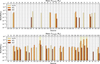 |
Fig. 7 The same as Fig. 6 but for S-bearing species, H2CS, SO2, and SiO. |
| In the text | |
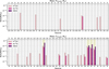 |
Fig. 8 Same as Fig. 6 but for N-bearing species, H13CN, HC15N, and HNCO. |
| In the text | |
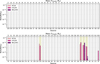 |
Fig. 9 Same as Fig. 6 but for N-bearing species, HC3N, CH3CN, and NH2CHO. |
| In the text | |
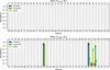 |
Fig. 10 Same as Fig. 6 but for O-bearing species, CH3OCH3, CH3OCHO, and HDCO. |
| In the text | |
|
Fig. 11 Peak-intensity images of the molecular species detected toward hot core 14A. The maps are ordered based on the frequency of the transition from left to right, top to bottom. The 1.2 mm continuum contours with contour levels of three, six, and nine times the σrms and the 50% 1.2 mm continuum contour are overlaid in each image for reference. Top is north and right is west. |
| In the text | |
|
Fig. 12 Comparisons of the derived temperatures (left) and abundances (right) from the current study and the literature. The top panels show a comparison of 4A and ST16 (Shimonishi et al. 2020), the middle panels show 6A and N105-2B, and the bottom panels show 6B and N105-2A (Sewiło et al. 2022). An error range of 40% is depicted for the temperatures and column densities from the current paper. |
| In the text | |
|
Fig. 13 Abundances of different molecular species for all the known hot cores in the LMC after scaling to the gas-to-dust mass ratio. The LMC hot cores are ST11 (Shimonishi et al. 2016a), 4A, 6A, 6B and 14A (this work), and N113 Al and N113 B (Sewiło et al. 2022). Black arrows show an upper limit estimation. An error range of 40% is shown on the abundances from the current paper. |
| In the text | |
|
Fig. 14 Comparisons of abundances for SO2, CH3OH, and CH3CN from observations of the seven hot cores detected in this galaxy and the LMC hot core models for the final hot core temperature of 100 K (top) and 200 K (bottom). The black curves show abundances over time for an initial dust temperature of 10 (dotted curve), 15 (dashed curve), 20 (larger dashed curve), and 25 K (the solid curve). The horizontal colored line shows the single abundance value for each hot core and follows the same color code as Fig. 13 (see the text for more details). |
| In the text | |
|
Fig. 15 Abundances of CH3OH, CH3CN, SO2, and SiO for all known hot cores in the SMC and LMC and for a selection of Galactic hot cores. The SMC hot cores are included, SO7 and SO9 (Shimonishi et al. 2023). The LMC hot cores are ST11 (Shimonishi et al. 2016a), 4A, 6A, 6B and 14A (this work), and N113 Al and N113 B (Sewiło et al. 2022). We selected four Galactic hot cores: an outer Galaxy hot core (Shimonishi et al. 2020), Orion Hot Core (HC) (Sutton et al. 1995), Sgr B2(N) (Nummelin et al. 2000), and W3(H2O) (Helmich & van Dishoeck 1997). The extent of each bar with a dotted pattern represents the abundances scaled to the Galactic metallicity. |
| In the text | |
|
Fig. 16 Comparisons of the abundances of CH3OH and CH3CN and SO2 and SO for the hot cores in the SMC (open green circles), LMC (red rectangles), and MW (black triangles for inner Galactic hot cores and gray triangle for outer Galactic hot core). Dashed lines show abundance relations of 1:1 for the top-right panel and 1:100 for the other panels. The dotted lines show a variation of a factor of ten above and below the relations described by the dashed lines. |
| In the text | |
|
Fig. 17 Three color composite image of the LMC combining 3.6 (blue), 4.5 (green), and 5.8 µm (red Meixner et al. 2006) images to highlight the position of the stellar bar. The dashed ellipse marks the bar region. The 20 ALMA fields from the current study are overlaid with white circles 15 times larger than the field of view of our ALMA observations. The fields accommodating hot cores are highlighted in yellow, including the YSO ST16 and N105 star-forming region. The field marked with a star shows the position of the new hot core detected in our survey. The location of the hot cores in N105 (Sewiło et al. 2022) and N113 (Sewiło et al. 2018) are marked with yellow rectangles. The hot cores ST11 (Shimonishi et al. 2016b) and ST16 (Shimonishi et al. 2020) are shown with yellow plus signs. The hot core ST11 with no COMs is the only hot core detected out of the LMC bar. |
| In the text | |
|
Fig. A.1 ALMA Band 6 observed spectra toward source 1A overlaid with the best-fit XCLASS model. Molecular transitions with definite detections (S/N > 5) are represented by solid black lines, while those with tentative detections (3 < S/N < 5) are denoted by dotted gray lines. Dotted red lines indicate transitions of molecules for which abundance upper limits are provided. (See Section 3.1 for more details.) |
| In the text | |
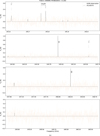 |
Fig. A.2 Same as Fig. A.1 but for source 2A. |
| In the text | |
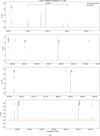 |
Fig. A.2 Same as Fig. A.1 but for source 2B. |
| In the text | |
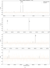 |
Fig. A.2 Same as Fig. A.1 but for source 2C. |
| In the text | |
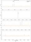 |
Fig. A.2 Same as Fig. A.1 but for source 2D. |
| In the text | |
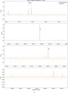 |
Fig. A.2 Same as Fig. A.1 but for source 2E. |
| In the text | |
 |
Fig. A.2 Same as Fig. A.1 but for source 2F. |
| In the text | |
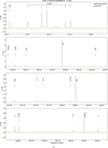 |
Fig. A.3 Same as Fig. A.1 but for source 3A. |
| In the text | |
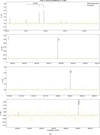 |
Fig. A.3 Same as Fig. A.1 but for source 3B. |
| In the text | |
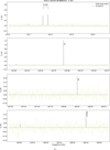 |
Fig. A.3 Same as Fig. A.1 but for source 3C. |
| In the text | |
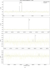 |
Fig. A.3 Same as Fig. A.1 but for source 3D. |
| In the text | |
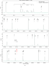 |
Fig. A.4 Same as Fig. A.1 but for source 4A. |
| In the text | |
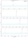 |
Fig. A.5 Same as Fig. A.1 but for source 5A. |
| In the text | |
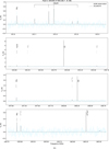 |
Fig. A.5 Same as Fig. A.1 but for source 5B. |
| In the text | |
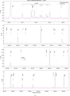 |
Fig. A.6 Same as Fig. A.1 but for source 6A. |
| In the text | |
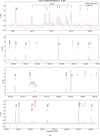 |
Fig. A.6 Same as Fig. A.1 but for source 6B. |
| In the text | |
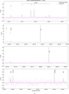 |
Fig. A.6 Same as Fig. A.1 but for source 6C. |
| In the text | |
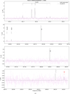 |
Fig. A.6 Same as Fig. A.1 but for source 6D. |
| In the text | |
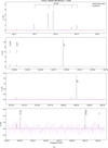 |
Fig. A.6 Same as Fig. A.1 but for source 6E. |
| In the text | |
 |
Fig. A.6 Same as Fig. A.1 but for source 6F. |
| In the text | |
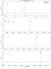 |
Fig. A.7 Same as Fig. A.1 but for source 7A. |
| In the text | |
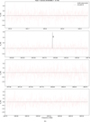 |
Fig. A.7 Same as Fig. A.1 but for source 7B. |
| In the text | |
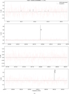 |
Fig. A.7 Same as Fig. A.1 but for source 7C. |
| In the text | |
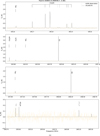 |
Fig. A.8 Same as Fig. A.1 but for source 8A. |
| In the text | |
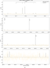 |
Fig. A.8 Same as Fig. A.1 but for source 8C. |
| In the text | |
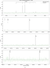 |
Fig. A.9 Same as Fig. A.1 but for source 9A. |
| In the text | |
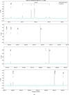 |
Fig. A.10 Same as Fig. A.1 but for source 10A. |
| In the text | |
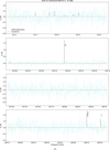 |
Fig. A.10 Same as Fig. A.1 but for source 10B. |
| In the text | |
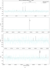 |
Fig. A.10 Same as Fig. A.1 but for source 10C. |
| In the text | |
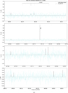 |
Fig. A.10 Same as Fig. A.1 but for source 10D. |
| In the text | |
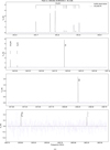 |
Fig. A.11 Same as Fig. A.1 but for source 11B. |
| In the text | |
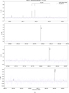 |
Fig. A.11 Same as Fig. A.1 but for source 11C. |
| In the text | |
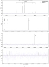 |
Fig. A.11 Same as Fig. A.1 but for source 11D. |
| In the text | |
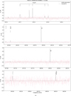 |
Fig. A.12 Same as Fig. A.1 but for source 12A. |
| In the text | |
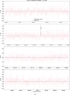 |
Fig. A.12 Same as Fig. A.1 but for source 12B. |
| In the text | |
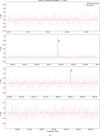 |
Fig. A.12 Same as Fig. A.1 but for source 12C. |
| In the text | |
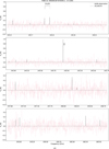 |
Fig. A.12 Same as Fig. A.1 but for source 12D. |
| In the text | |
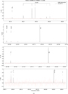 |
Fig. A.13 Same as Fig. A.1 but for source 13A. |
| In the text | |
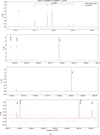 |
Fig. A.13 Same as Fig. A.1 but for source 13C. |
| In the text | |
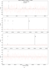 |
Fig. A.13 Same as Fig. A.1 but for source 13D. |
| In the text | |
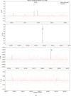 |
Fig. A.13 Same as Fig. A.1 but for source 13E. |
| In the text | |
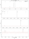 |
Fig. A.13 Same as Fig. A.1 but for source 13F. |
| In the text | |
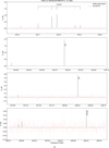 |
Fig. A.13 Same as Fig. A.1 but for source 13G. |
| In the text | |
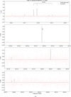 |
Fig. A.13 Same as Fig. A.1 but for source 13H. |
| In the text | |
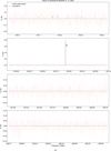 |
Fig. A.13 Same as Fig. A.1 but for source 13K. |
| In the text | |
|
Fig. A.14 ALMA Band 6 observed spectra toward source 14B with no emission line detections. (See Section 3.1 for more details.) |
| In the text | |
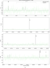 |
Fig. A.15 Same as Fig. A.1 but for source 15A. |
| In the text | |
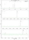 |
Fig. A.15 Same as Fig. A.1 but for source 15B. |
| In the text | |
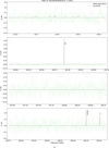 |
Fig. A.15 Same as Fig. A.1 but for source 15C. |
| In the text | |
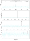 |
Fig. A.16 Same as Fig. A.1 but for source 16B. |
| In the text | |
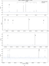 |
Fig. A.17 Same as Fig. A.1 but for source 17A. |
| In the text | |
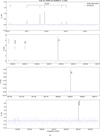 |
Fig. A.18 Same as Fig. A.1 but for source 18A. |
| In the text | |
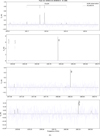 |
Fig. A.18 Same as Fig. A.1 but for source 18B. |
| In the text | |
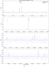 |
Fig. A.18 Same as Fig. A.1 but for source 18C. |
| In the text | |
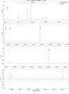 |
Fig. A.19 Same as Fig. A.1 but for source 19A. |
| In the text | |
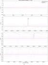 |
Fig. A.19 Same as Fig. A.1 but for source 19C. |
| In the text | |
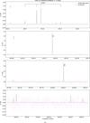 |
Fig. A.19 Same as Fig. A.1 but for source 19D. |
| In the text | |
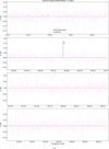 |
Fig. A.20 Same as Fig. A.1 but for source 20A. |
| In the text | |
|
Fig. B.1 Comparisons of the LTE and non-LTE fit for two CH3OH lines at 241.767 and 241.791 GHz. |
| In the text | |
|
Fig. C.1 Comparisons of abundances for CS, SO, SiO, H2CS, HNCO, and NH2CHO from observations of the seven hot cores detected in the LMC and the LMC hot core models for the final hot core temperature of 100 K. The black curves show abundances over time for initial dust temperatures of 10 (dotted line), 15 (dashed curve), 20 (larger dashed curve), and 25 K (solid curve; this curve does not necessarily appear in the range of abundances in the plot). The horizontal colored line shows the single abundance value for each hot core and follows the same color code as Fig. 13 (see the text for more details). |
| In the text | |
|
Fig. C.2 Same as Fig. C.1 but for the LMC hot core models for the final hot core temperature of 200 K. |
| In the text | |
Current usage metrics show cumulative count of Article Views (full-text article views including HTML views, PDF and ePub downloads, according to the available data) and Abstracts Views on Vision4Press platform.
Data correspond to usage on the plateform after 2015. The current usage metrics is available 48-96 hours after online publication and is updated daily on week days.
Initial download of the metrics may take a while.