| Issue |
A&A
Volume 664, August 2022
|
|
|---|---|---|
| Article Number | A154 | |
| Number of page(s) | 22 | |
| Section | Interstellar and circumstellar matter | |
| DOI | https://doi.org/10.1051/0004-6361/202243532 | |
| Published online | 24 August 2022 | |
CHEMOUT: CHEMical complexity in star-forming regions of the OUTer Galaxy
II. Methanol formation at low metallicity
1
INAF – Osservatorio Astrofísico di Arcetri,
Largo E. Fermi 5,
50125
Florence, Italy
e-mail: This email address is being protected from spambots. You need JavaScript enabled to view it.
2
Centre for Astrochemical Studies, Max-Planck-Institute for Extraterrestrial Physics,
Giessenbachstrasse 1,
85748
Garching, Germany
3
I. Physikalisches Institut, Universitat zu Köln,
Zülpicher Str. 77,
50937
Köln, Germany
4
Centro de Astrobiología (CSIC-INTA),
Ctra. de Ajalvir Km. 4, Torrejón de Ardoz,
28850
Madrid, Spain
5
INAF – IAPS,
via Fosso del Cavaliere, 100,
00133
Roma, Italy
6
Dipartimento di Chimica “Giacomo Ciamician”, Università di Bologna,
Bologna, Italy
7
INAF – Osservatorio di Astrofísica e Scienza dello Spazio,
Via Gobetti 93/3,
40129
Bologna, Italy
Received:
12
March
2022
Accepted:
17
May
2022
Abstract
Context. The outer Galaxy is an environment with a lower metallicity than the regions surrounding the Sun and for this reason the formation and survival of molecules in star-forming regions located in the inner and outer Galaxy are expected to be different.
Aims. To gain understanding of how chemistry changes throughout the Milky Way, it is crucial to observe the outer star-forming regions of the Galaxy in order to constrain models adapted for lower metallicity environments.
Methods. The project ‘chemical complexity in star-forming regions of the outer Galaxy’ (CHEMOUT) is designed to address this problem by observing a sample of 35 star-forming cores at Galactocentric distances of up to ~23 kpc with the Institut de RadioAstronomie Millimétrique (IRAM) 30 m telescope in various 3 mm and 2 mm bands. In this work, we analyse observations of methanol (CH3OH), one of the simplest complex organic molecules and crucial for organic chemistry in star-forming regions, and of two chemically related species, HCO and formaldehyde (H2CO), towards 15 out of the 35 targets of the CHEMOUT sample. More specifically, we consider only the targets for which both HCO and H2CO were previously detected, which are precursors of CH3OH.
Results. We detected CH3OH in all 15 targets. The emission is associated with an extended envelope, as the average angular size is ~47″ (i.e. ~2.3 pc at a representative heliocentric distance of 10 kpc). Using a local thermodynamic equilibrium approach, we derive CH3OH excitation temperatures in the range ~7–16 K and line widths ≤4 km s−1, which are consistent with emission from a cold and quiescent envelope. The CH3OH fractional abundances with respect to H2 range between ~0.6 × 10⁻⁹ and ~7.4 × 10⁻⁹. These values are comparable to those found in star-forming regions in the inner and local Galaxy. H2CO and CH3OH show well-correlated line velocities, line widths, and fractional abundances with respect to H2, indicating that their emission originates from similar gas. These correlations are not seen with HCO, suggesting that CH3OH is likely more chemically related to H2CO than to HCO.
Conclusions. Our results have important implications for the organic and possibly pre-biotic chemistry occurring in the outermost star-forming regions of the Galaxy, and can help to set the boundaries of the Galactic habitable zone.
Key words: stars: formation / ISM: clouds / ISM: molecules
© F. Fontani et al. 2022
 Open Access article, published by EDP Sciences, under the terms of the Creative Commons Attribution License (https://creativecommons.org/licenses/by/4.0), which permits unrestricted use, distribution, and reproduction in any medium, provided the original work is properly cited.
This article is published in open access under the Subscribe-to-Open model. This email address is being protected from spambots. You need JavaScript enabled to view it. to support open access publication.
1 Introduction
The outer Galaxy (OG) is the portion of the Milky Way located beyond the Sun, that is at a distance from the Galactic centre, RGC, between approximately the Solar circle (at ~8.34 kpc; Reid et al. 2014) and ~28 kpc (Digel et al. 1994). The inner and outer Galaxy show significantly different chemical properties. First, in the outer Galaxy, the overall content of elements heavier than helium, which defines the metallicity, is lower than solar metallicity (e.g. Wenger et al. 2019). The elemental abundances of oxygen, carbon, and nitrogen, namely the three most abundant elements in the Universe after hydrogen and helium, decrease linearly (in logarithmic scale) as a function of RGC (e.g. Esteban et al. 2017; Arellano-Córdova et al. 2020; Méndez-Delgado et al. 2022). Because of the lower abundances of heavy elements therein with respect to the solar ones and those of the inner Galaxy, it has been suggested that the outer Galaxy is not suitable for forming planetary systems in which Earth-like planets could be born and might be capable of sustaining life (Prantzos 2008; Ramírez et al. 2010). The so-called Galactic habitable zone (GHZ) in the Milky Way is currently defined as an annular region of about 2 kpc in width centred at RGC 8 kpc, where the metallicity is appropriate to form Earth-like planets and where the occurrence of disruptive events such as supernovae is limited (Spitoni et al. 2014, Spitoni et al. 2017). Because of this, and also because of the fact that star-forming regions in the outer Galaxy are on average further away from us, the study of the formation of stars and planets, as well as the
search for the basic bricks of life that could have favoured the emergence thereof, has so far been focussed almost exclusively on the inner Galaxy, where the metallicity is solar or supersolar.
This scenario has been challenged by recent observational results. First, the occurrence of Earth-like planets does not seem to depend on the Galactocentric distance (e.g. Buchhave et al. 2012; Maliuk & Budaj 2020). This indicates that planets capable of hosting life can be found even at metallicities lower than solar, depending also on the dynamical history of the host stars (Dai et al. 2021), which is likely to be different in the inner and outer Galaxy. Second, observations performed with the Atacama Large Millimeter Array (ALMA) towards the Large and Small Magellanic Clouds (LMC and SMC; Shimonishi et al. 2018; Sewilo et al. 2018, Sewilo et al. 2022), two external galaxies with metallicities of approximately three and five times lower than solar, respectively, led to the detection of emission of complex organic molecules (COMs), which are organic species with more than five atoms. This finding, and the recent discovery of a hot molecular core at RGC ~19 kpc that is rich in COMs (Shimonishi et al. 2021), clearly suggest that the astrochemical processes that can lead to species of pre-biotic interest can be also found in metal-poor environments. In particular, methanol (CH3OH), a simple but crucial COM, was detected in star-forming regions associated with both the LMC and the SMC, as well as with star-forming regions in the Milky Way up to RGC ~ 20 kpc (Bernal et al. 2021). Methanol is thought to be a crucial species for prebiotic chemistry as it is considered a possible parent species for larger organic molecules in both gas and ice (e.g. Charnley et al. 1992; Öberg et al. 2009; Chen et al. 2013; Chuang et al. 2016). Its presence therefore paves the way for the synthesis of more complex organic species.
In the present paper, we study the emission of methanol, the formyl radical (HCO), and formaldehyde (H2CO) from 15 candidate high-mass star-forming regions in the OG with RGC in between 13.1 and 19 kpc. Although the OG is more extended than 19 kpc (see above), the RGC range studied in this work is where the metallicity gradients are better constrained by observations (e.g. Esteban et al. 2017; Kovtyukh et al. 2022); beyond 20 kpc, the metallicity gradients are much less well constrained (Spina et al. 2022). HCO and H2CO are precursors of methanol (Watanabe & Kouchi 2002) and of other COMs relevant for prebiotic chemistry such as formamide (e.g. Fedoseev et al. 2016), glycolaldehyde, and ethylene glycol (Bennet & Kaiser 2007; Woods et al. 2012, 2013; Chuang et al. 2016; Rivilla et al. 2017, 2019). These observations can therefore indicate whether or not the formation pathways of CH3OH, known to be efficient starting from Solar-like metallicities, are also efficient in the lower metallicity environment of the OG.
Our targets are part of the project ‘chemical complexity in the outer Galaxy’ (CHEMOUT) – an observational project described by (Fontani et al. 2022, hereafter paper I) and performed with the Institut de RadioAstronomie Millimétrique (IRAM) 30m telescope1 – the aim of which is to study the chemical complexity in the low-metallicity environment of the OG. Our sample and observations are described in Sect. 2. The data analysis is described in Sect. 3. The results are presented in Sect. 4 and discussed in Sect. 5.
Source list and parameters taken from paper I.
2 Sample and observations
We targeted 15 sources extracted from the sample described in paper I. This sample is made of 35 targets selected from Blair et al. (2008), who searched for formaldehyde emission with the Arizona Radio Telescope (ARO) 12m telescope in dense molecular cloud cores in the OG. All cores are associated with IRAS colours typical of star-forming regions. The targets of this work, which are listed in Table 1, were selected because both HCO (paper I) and H2CO (Blair et al. 2008) were detected in their emission spectra, and their RGC cover a wide range among the sources for which HCO was detected (see paper I). In the same
table, we give coordinates and other source parameters useful for the analysis, such as H2 column densities estimated from previous works, and both Galactocentric and heliocentric (d) distances estimated in paper I.
The observed lines are listed in Table 2. All parameters of the CH3OH and H2CO lines are taken from the Cologne Database for Molecular Spectroscopy (CDMS2, Endres et al. 2016), while those of the HCO lines are taken from the Jet Propulsion Laboratory (JPL3, Pickett et al. 1998).
Observations of the CH3OH and H2CO lines listed in Table 2 were performed with the IRAM-30m telescope in two observing runs (July and September, 2021; project 042-21). We used the 3 and 2 mm receivers simultaneously. We note that 11 of our 15 targets were recently observed by Bernal et al. (2021) with the ARO telescope, who were searching for the same CH3OH lines at 3 mm, and found them for 10 of the sources. In this work, we re-observe these lines with higher sensitivity (rms of ~5–10 mK versus ~ 17–20 mK, in main beam temperature units) and higher angular resolution (25″ versus 63″). Moreover, we add to the analysis the 2 mm lines, which have upper level energies of up to ~50 K, and therefore allow us to constrain the CH3OH parameters – in particular Tex – more accurately than with the 3 mm lines only, for which the range of upper level energy is ~7–28 K (Table 2). Sources WB89-006, WB89-789, WB89-035, and WB89-080 were observed in both bands for the first time.
The Local Standard of Rest (LSR) velocities used to centre the spectra are listed in Table 1 of paper I. The observations were made in wobbler-switching mode with a wobbler throw of 220″. Pointing was checked (almost) every hour on nearby quasars or bright HII regions. Focus was checked on the planet Saturn at the start of observations and after sunset. The data were calibrated with the chopper wheel technique (see Kutner & Ulich 1981), with a calibration uncertainty of about 10%. The telescope half power beam width (HPBW) is ~25″ and ~17″ in the 3 and 2 mm bands, respectively. The spectra were obtained in main beam temperature units with the fast Fourier transform spectrometer with a channel width of 200 kHz (FTS200), providing a spectral resolution of ~0.6 km s−1 and -0.4 km s−1 at 3 and 2 mm, respectively. The total bandwidth observed is 90400–98 180 MHz and 140 720–148 500 MHz at 3 and 2 mm, respectively. The 1σ rms noise level for each spectrum around the CH3OH lines is given in Table 1.
The observations of the HCO lines listed in Table 2 were performed with the IRAM-30m telescope in the observing runs described in paper I. We refer to that paper for any observational and technical details related to these data.
3 Data reduction and analysis
The first steps of the data reduction (e.g. average of the scans, baseline removal, flag of bad scans and channels) were made with the Continuum and Line Analysis Single-dish Software (class) package of the Grenoble Image and Line Data Analysis Software (GILDAS4) using standard procedures. The baseline-subtracted spectra in main beam temperature (TMB) units were fitted with the MAdrid Data CUBe Analysis (MADCUBA5, Martín et al. 2019) software.
The transitions of HCO, H2CO, and CH3OH in the bands described in Sect. 2 were identified via the SLIM (Spectral Line Identification and LTE Modelling) tool of MADCUBA. The lines were fitted with the AUTOFIT function of SLIM. This function produces the synthetic spectrum that best matches the data assuming a constant excitation temperature (Tex) for all transitions. The other input parameters are: total molecular column density (Ntot), radial systemic velocity of the source (V), line full-width at half-maximum (FWHM), and angular size of the emission (θS). AUTOFIT assumes that V, FWHM, and θS are the same for all transitions. These input parameters have all been left free except θS. More specifically, θS can be computed for the CH3OH and H2CO lines observed also with the ARO-12m telescope by comparing the line intensities obtained with the two telescopes.
As mentioned in Sect. 2, Bernal et al. (2021) detected the same 3 mm CH3OH transitions in 10 of our 15 targets. Assuming that the brightness temperature distribution is Gaussian, and the same for the beam of the two telescopes, and that there is no contamination from other sources when moving from the smaller to the larger beam, one finds that the angular size of the emission is given by (see also Eqs. (2) and (3) in Fontani et al. 2002):
 (1)
(1)
where θAro and θirAm are the half power beam widths of the two telescopes at the frequency of the observed lines, and 
and  are the main beam brightness temperature at line peak obtained with the ARO-12m and IRAM-30m telescope, respectively. We compare the intensity of the strongest transition, namely the 2(0,2)–1(0,1) A+ transition at ~ 96741 MHz (Table 2). ΘARO and ΘIRAM are 63″ and 25″, respectively, at -97 GHz. For each source,
  was obtained by fitting the line with a single Gaussian in class, and
  was obtained by converting the line intensity given in Table 3 of Bernal et al. (2021) to TMB units by dividing it by a factor of 0.61. This conversion factor was taken from Appendix C.3 of the ARO-12m user manual.
  , and the associated θS are reported in Table 3. For the sources for which the second strongest CH3OH line is detected in both works, that is the 2(1,2)–1(1,1) E2 transition at ~96739 MHz, we find angular sizes that are consistent within the uncertainties.
We performed the same analysis for the  transition of H2CO at ~140 840 MHz, observed both in this work and in Blair et al. (2008). To convert the line intensities given in Table 1 of Blair et al. (2008) to TMB units, we divided their values by 0.86. ΘARO and ΘIRAM are 44″ and 17″, respectively, at ~140 GHz. The obtained θS, and the intensities of the lines used to derive them, are listed in Table 4.
For both molecules in all sources, θS is larger (in some cases much larger) than the IRAM-30m beam. This indicates that the observed transitions trace an extended envelope of the cores. More specifically, from the heliocentric distances given in Table 1, we derive that the linear size of the emitting region is ~1.5–5 pc for CH3OH and ~0.9–6 pc for H2CO. In Fig. 1, we plot the linear diameter, D, of H2CO against that of CH3OH, from which we see that D[CH3OH] and D[H2CO] are positively correlated. There are no systematic similarities or differences because D[CH3OH] is equal to D[H2CO] within the errors in three sources, is larger in five sources, and is smaller in two sources. Hence, this comparison indicates that the two tracers are associated with extended envelopes of comparable dimensions within a factor of 2.
In the analysis performed with madcuba, for the five sources for which θS of CH3OH could not be derived from the data, we assume the average angular size of the other sources (i.e. 47″). We adopted this simplified approach because the five targets have similar heliocentric distances (in the range 8.9–12.2 kpc). However, we checked how the results would change if adopting for each source the angular size obtained from the average linear diameter computed from the sources with measured angular sizes, that is ~2.8 pc. Repeating the fits fixing θS to these angular sizes, we obtain best-fit results that are consistent within the uncertainties with the results obtained from the average angular size for both Tex and Ntot. For HCO, because the size of the emission is unknown in the studied lines, we assume that the emission fills the telescope beam. This assumption is justified by the fact that the upper level energies of the observed transitions are very low (~4 K, Table 2), and that HCO is found to trace the extended envelope of star-forming cores (e.g. Rivilla et al. 2019).
The best-fit parameters obtained for CH3OH are listed in Table 3, and those obtained for H2CO and HCO are given in Tables 4 and 5, respectively. For HCO, because the four observed lines have the same upper level energies, we were not able to derive Tex from the data. We therefore had to fix Tex. We discuss the assumed Tex for HCO in Sect. 4.3.
CH3OH line parameters.
4 Results
4.1 Methanol
We detected CH3OH emission in both observing bands towards all targets. The observed spectra and their best fits (superimposed on them) are shown in Figs. A.1 and A.2. The residuals,
shown in Fig. A.3, are generally lower than or comparable to the 3σ rms noise (Table 1) towards all the methanol lines except for five targets, namely WB89-391, WB89-437, WB89-621, WB89-006, and WB89-076, in which at least one CH3OH line is significantly underestimated by the best fit. This cannot be due to (large) optical depth effects because the best-fit opacities provided by madcuba are always below 0.1. However, considering that we assume a constant Tex for all transitions, this can be due to marginal deviations from this simplified approach. As stated in Sect. 2, 11 out of our 15 targets were already observed in CH3OH at 3 mm by Bernal et al. (2021) with the ARO telescope, and 10 of them were detected at 3 mm. In this work, we confirm all the detections of these latter authors and, thanks to our higher sensitivity, we confirm their tentative detection of CH3OH claimed towards WB89-283. Moreover, we also detect the fainter 3 mm transitions at rest frequencies 96744.545 and 96 755.501 MHz (Table 2), which were observed but undetected towards some targets in Bernal et al. (2021).
We find Tex in the range 7-16.4 K, and FWHM of the lines in the range ~1–4 kms−1 (Table 1). These values confirm what was already suggested by Bernal et al. (2021), and by the estimated angular sizes, namely that the emission is dominated by the cold and (relatively) quiescent gaseous envelope of the cores. This result is also in agreement with the low excitation energy of the transition from which θS is estimated (Eu = 7 K, see Table 2). Bernal et al. (2021) also measured the kinetic temperatures from a non-LTE analysis, and derived values in the range 10–25 K. This would indicate that the methanol emission could be subthermally excited in several sources. It is not trivial to deduce whether or not the methanol lines are subthermally excited, and if so by how much, because the calculation of the critical densities of the CH3OH lines is not straightforward. As discussed by Shirley (2015), the ‘typical’ expression that includes only the Einstein coefficient for spontaneous emission and the collisional coefficient is valid only in a two-level approximation, which is not appropriate for molecules with a spectrum as complex as that of methanol.
We used RADEX online7 to test possible differences with respect to a non-LTE approach, especially for the sources for which our fitting procedure gives the highest residuals. For example, the intensity of the 3 mm lines in WB89-621 belonging to the −A and −E species can be reproduced assuming a kinetic temperature, Tk, of 15 K, a line width equal to the observed one (1.74 kms−1, Table 3), and a H2 volume density, n(H2), of 3 × 106 cm−3. Tk and n(H2) are similar to the values obtained by Bernal et al. (2021) with their non-LTE approach. The resulting Tex and total column density, Ntot, (derived as the sum of the column density of the −A and −E species) are 14 K and 6 × 1013 cm−2, respectively, consistent with the estimates obtained with our approach (Tex~12 K and Ntot ~ 8.5 × 1013 cm−2). The excitation temperatures and column densities are both comparable for the −A and −E species.
We note that a n(H2) of ~106 cm−3 may not be appropriate for the angular scales we are probing. From the H2 column densities and diameters provided in Table 1, for WB89-621 we derive a n(H2) of ~3 × 103 cm−3 when smoothed on the methanol source size of 42″. In RADEX, we therefore fixed n(H2) to ~3 × 103 cm−3, the FWHM to that observed, and Tk ~ 15 K. The line intensities can be reproduced with Ntot ~ 1.3 × 1014 cm−2 (7.2 × 1013 cm−2 for the -A species, 6 × 1013 cm−2 for the −E species), which is higher but still roughly consistent (within a factor 1.5) with the estimate found in the LTE approach also in this case. The excitation temperature is now ~4 K, indicating subthermal excitation. However, even with different combinations of Tk, n(H2), and Tex, Ntot must always be close to the value obtained in the LTE approach to reproduce the observed line intensities. Similar results can be obtained towards WB89-391, WB89-437, WB89-006, and WB89-076, for which a non-LTE approach considering n(H2) in the range 103–104 cm−3 always needs values of Ntot consistent with the results obtained in LTE to reproduce the line intensities. In general, the non-LTE approach does not significantly improve the intensity ratios between −A and −E lines with respect to the LTE approach, except when using the unrealistic option of a different H2 volume density for − A and − E species. Furthermore, the excitation temperatures for − A and − E species appear to be consistent with each other, and even assuming − A and −E ratios smaller than one does not significantly improve the fit results either.
This, and the general good agreement between the fits and the observed spectra (Figs. A.1-A.3), shows that our LTE analysis provides accurate total column densities, even if some transitions are likely subthermally excited.
Shimonishi et al. (2021) found that one of our targets, namely WB89-789, harbours a hot core in which the kinetic temperature measured with ALMA is higher than 100 K at scales ≤0.03 pc, obtained from CH3OH lines. However, Shimonishi et al. (2021) estimated Tex mostly from transitions with Eu ≥ 100 K, which is certainly arising from the inner hot core. We produced a synthetic spectrum with MADCUBA, fixing Tex to 100 K, θS to 0.6″ (corresponding to 0.03 pc at the source heliocentric distance of 11 kpc), and the column density to the value found by Shimonishi et al. (2021), that is ~1.9 × 1016 cm−2. As expected, the resulting spectrum is within the noise level of our data, and therefore does not give a significant detectable contribution to the emission observed with the IRAM-30m telescope. This confirms that our observations trace only the external envelope of the hot core, and that in this target, and potentially also in the others, higher angular resolution observations are needed to study the warmer, more compact gaseous components.
The CH3OH total column densities obtained towards our targets are in the range ~0.25 × 10¹³ and ~8.5 × 1013 cm−2 (Table 3). These values are consistent within a factor of ~2 with those estimated by Bernal et al. (2021) in the common targets, once a beam dilution factor is applied to our values to match their beam of 63″.
H2CO line parameters.
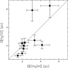 |
Fig. 1 Comparison between linear diameters obtained for CH3OH (x-axis) and H2CO (y-axis). Both diameters are calculated from the angular diameters given in Tables 3 and 4, respectively, and the source heliocentric distances in Table 1. The dashed line is the locus where D[CH3OH] = D[H2CO]. |
4.2 Formaldehyde
The two formaldehyde lines listed in Table 2, fitted and analysed as described in Sect. 3, are all clearly detected, as seen in the spectra of Figs. A.4 and A.5. The line at ~140.8 GHz was detected in all sources by Blair et al. (2008) with an angular resolution of 44″. We confirm all their detections and add in the analysis the line at ~145.6 GHz. Some targets present hints of non-Gaussian high-velocity wings in the spectra of both transitions: WB89-437, WB89-621, 19423+2541, and WB89-080. All these sources were known to have high-velocity wings in the HCO+ J = 1–0 line (paper I). A second velocity feature towards 19383+2711, already found in HCO+, is clearly detected also in H2CO. Two targets, WB89-380 and WB89-006, show hints of two peaks in the ~140.8 GHz line. In WB89-380, such a profile is not seen in the other line at ~145.6 GHz, suggesting that it could be due to self-absorption. Instead, a similar profile is seen towards the other transition in WB89-006, suggesting that in this case a second velocity feature could also be responsible for the second velocity peak. However, in all cases the residuals of the Gaussian fits are low.
The best-fit parameters are given in Table 4. The total column densities are in the range 0.6–9.3 × 1013 cm−2 which is similar to the CH3OH ones. The excitation temperatures are in the range 25–45 K, which is significantly larger than those measured in CH3OH (Table 3). We discuss this result further in Sect. 5.1.
4.3 Formyl radical
The four HCO transitions listed in Table 2 were fitted and analysed as described in Sect. 3. The observed spectra and the best fit superimposed on them are shown in Figs. A.6 and A.7. In most sources, three out of the four transitions are clearly detected at a significance level of ~3σ rms or higher, while that at 86.80578 GHz, having the lowest line strength, is clearly detected only towards WB89-380 and WB89-391.
The best LTE fit parameters are given in Table 5. As mentioned in Sect. 3, Tex could not be derived from the observations because the energies of the transitions were the same. Thus, as a first-order approach, we fixed Tex to the values obtained from CH3OH. We obtained FWHM in between 1.15 and 6.5 kms−1, although the latter value, obtained towards 19383+2711, is very likely affected by the presence of a second unresolved velocity feature (clearly detected in HCO+ and c-C3H2; see paper I). Excluding this case, the measured FWHMs are in between 1.15 and 3.3 km s−1. The HCO total column densities are in the range 0.6-9.3 × 1012 cm−2, and are therefore an order of magnitude lower than those of CH3OH and H2CO.
An alternative choice for Tex would be that computed from H2CO, which is likely closer to LTE conditions, as demonstrated by the good agreement between the LTE fits and the spectra (see Figs. A.4 and A.5). However, as we discuss in Sect. 5.1, in light of the significantly narrower line widths at half maximum, HCO is very likely associated with an envelope that is more extended and less turbulent than that traced by both H2CO and CH3OH. The excitation temperature of H2CO therefore likely represents the gas kinetic temperature of a region more turbulent (and likely more compact) than that traced by HCO. Therefore, the smaller Tex derived from the (likely) subthermally excited CH3OH lines could be closer to the real excitation conditions of HCO. In summary, it is not clear ‘a priori’ which of the two Tex is most appropriate, and therefore we decided to fit the HCO lines also fixing Tex to that of H2CO. The results are given in Table B.1, and the alternative fits are shown in Figs. A.8 and A.9.
With respect to the results performed using the Tex of CH3OH (Table 5), the line widths at half maximum and peak velocities are almost identical, while Ntot are systematically higher by a moderate factor (≤3) for all sources except for WB89-789 and 19423+2541, for which they are higher by factors of ~5.6 and –3.8, respectively. Because the alternative fits do not seem to reproduce the observed spectra better than the first-order ones (compare Figs. A.6-A.7 with Figs. A.8-A.9), it is not clear which approach is more accurate. In the following sections, we consider the results derived from Tex of CH3OH, which we believe to better represent an envelope that is more extended than that traced by H2CO, bearing in mind that they have to be considered as lower limits if the actual Tex of HCO are higher.
HCO line parameters.
5 Discussion
5.1 Excitation temperatures, FWHM, and V of the lines
Inspection of Tables 3-5 suggests that some molecular parameters obtained from CH3OH, HCO, and H2CO are similar, while others are significantly different. We first examine the best-fit Tex, FWHM, and V.
The excitation temperatures measured from H2CO are larger than those estimated from CH3OH, and no correlation is found between the two Tex estimates, as can be seen from Fig. 2. We also investigated whether the sources with higher Tex – and those that are therefore potentially warmer if Tex is representative of Tk – are associated with gas emitting lines with larger FWHM that is therefore more turbulent. As can be noted from the middle and bottom panels in Fig. 2, we do not find any statistically significant correlation between Tex and FWHM estimated from both H2CO and CH3OH. The different Tex may be explained if CH3OH traces gas that is colder than that traced by H2CO. On the other hand, the best-fit V for H2CO and CH3OH are very similar, as they differ by less than ~0.2 km s−1 in all targets (Fig. 3, top panel), and also the best-fit FWHMs are very well correlated (Fig. 3, bottom panel). This suggests that the gas emitting H2CO and CH3OH could be made up of layers, or portions,
characterised by different (excitation) temperatures but belonging to a region kinematically and spatially coherent.
The best-fit V derived for HCO and CH3OH are different by up to ~0.9 km s−1, which is more than three times the difference in velocity between CH3OH and H2CO (Fig. 3, top panel). Even not including WB89-006, for which the difference is the largest (~0.9 km s−1), the range is still ~0.4 km s−1, which is twice that found for H2CO and CH3OH. Also, the lines FWHM derived for HCO do not appear correlated to those of CH3OH, (Fig. 3, middle panel), indicating that the observed HCO emission could arise from material that is kinematically and therefore spatially different from that responsible for the CH3OH and H2CO emission. As discussed in Rivilla et al. (2019), HCO can be formed on dust grains through hydrogenation of iced CO (Tielens & Hagen 1982; Dartois et al. 1999; Watanabe & Kouchi 2002; Bacmann & Faure 2016), and in this case be the progenitor of H2CO and CH3OH, but also in the gas phase from atomic C and H2O (Bacmann & Faure 2016; Hickson et al. 2016; Rivilla et al. 2019). In this case, the HCO emission should arise predominantly from an envelope in which C is still significantly in atomic form, which is likely more extended and diffuse than the region from where the emission of both H2CO and CH3OH arises, which requires most of the C to be locked in CO, where it would therefore be more dense.
Furthermore, as discussed by Pauly & Garrod (2018), even in iced HCO, hydrogenation of HCO will form either H2CO or H2 + CO with equal probability, while, once formed, H2CO is fairly robust and can quickly form CH3O or CH2OH, from which H addition to finally form CH3OH is fast. For these reasons, H2CO and CH3OH in cold environments are likely more related than HCO and CH3OH, and our observational results are in agreement with this scenario. H2CO can also form in the gas phase (unlike CH3OH) in regions where a significant fraction of C is not yet locked into CO. Our findings suggest that, in these regions, most of the C is indeed in the form of CO, possibly because the present-day O/C ratio is larger than in the solar neighbourhood. We discuss this point further in Sect. 5.4.
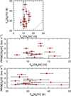 |
Fig. 2 Tex and FWHM comparison for CH3OH, H2CO, and HCO. Top panel: comparison between the best-fit Tex estimated from H2CO and CH3OH. The dotted line indicates Tex[H2CO] = Tex[CH3OH]. Middle and bottom panels: Tex against FWHM measured from H2CO (middle) and from CH3OH (bottom). The CH3OH and H2CO parameters are given in Tables 3 and 4, respectively. |
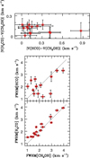 |
Fig. 3 Velocity and FWHM comparison for CH3OH, H2CO, and HCO. Top panel: velocity difference between H2CO and CH3OH versus the difference between HCO and CH3OH. Middle and bottom panels: comparison between the FWHM measured for HCO and CH3OH (middle) and that measured from CH3OH and H2CO (bottom). The dotted line indicates FWHM[HCO] = FWHM[CH3OH] or FWHM[H2CO] = FWHM[CH3OH]. The HCO data for 19383+2711 is missing from all panels, for which the resulting fit parameters are affected by the unresolved second velocity feature (see Sect. 4.3). |
5.2 Fractional abundances of CH3OH
From the NCO(H2) listed in Table 1, we estimate the methanol fractional abundances with respect to H2, X[CH3OH]. These are listed in Table 6 and are in the range 1.1–5.8 × 10⁻⁹. These values are obtained by smoothing the column densities to the largest of the two angular sizes over which they are computed, which are θS for CH3OH (Table 3) and 44″ (i.e. the beam size) for NCO(H2).
We derived CH3OH abundances also using N(H2) computed from Herschel Hi-GAL data, NHer(H2), when available (Elia et al. 2021). The NHer(H2) given in Hi-GAL, and computed from the spectral energy distribution of the sources, are averaged within the continuum angular sizes, θc, computed from the Herschel 250 µm emission as explained in Elia et al. (2021). Both NHer(H2) and θc are listed in Table 1, and the resulting X[CH3OH] is shown in Table 6. The two estimates of X[CH3OH] agree with each other within a factor of four, even though the computed range in this case is larger (0.6–7.4 × 10⁻⁹).
We compared our results with star-forming regions at different metallicities: inner and local Galactic targets (representative of solar and supersolar metallicities), and OG cores and extra-galactic sources (representative of subsolar metallicities). The list of these sources, with their abundances and reference works, is given in Table 6. Because we cannot yet robustly constrain the nature and evolutionary stage of our targets, we considered a large variety of star-forming regions, from early cold cores embedded in infrared-dark clouds (IRDCs), to protostellar objects and hot molecular cores in warmer and more evolved high-mass star-forming regions (HMSFs). Comparing our sources with targets located in the local and inner Galaxy (Table 6), we do not find significant or systematic differences. The clearest difference is seen towards the IRDC cores studied by Vasyunina et al. (2014): for these objects the CH3OH abundances are on average higher than in our targets. However, our values overlap with the lower edge of their measured range. Moreover, the HMSF cores observed with similar angular resolutions to ours (e.g. Minier & Booth 2002; van der Tak et al. 2000; Gerner et al. 2014) show values that overlap with ours.
Comparing our results to those obtained in other low-metallicity environments, we find very good agreement with the OG star-forming cores observed by Bernal et al. (2021), as expected because the two samples have several sources in common. Interestingly, the CH3OH abundances measured in our study are lower than those measured towards the hot core embedded in WB89-789 (1.7 × 10⁻⁷), as well as in the Small and Large Magellanic Clouds (~10−8). However, this difference is likely due to the higher excitation of the lines used to derive the abundances of the mentioned regions, which have upper energies that are typically much larger than 100 K. These lines are associated with warmer (and likely more compact) gas – enriched in CH3OH upon evaporation of dust grain mantles – than that traced by the lines observed in this work, which is more likely associated with a colder envelope where a lot of CH3OH is still
frozen. Interestingly, Shimonishi et al. (2018) and Sewilo et al. (2018) claim that the CH3OH emission arises from hot molecular cores embedded inside both the LMC and the SMC.
Of course, care needs to be taken in these comparisons, given the large number of important assumptions, such as the assumed gas-to-dust ratio to derive the N(H2) column density from the continuum, or the CO-H2 conversion factor used to derive N(H2) from CO, which can significantly influence the abundance estimates (see e.g. Nakanishi & Sofue 2006; Pineda et al. 2013). The probed linear scales are also very different in several cases.
Abundances of CH3OH calculated in this work, and towards other star-forming regions both in the Galaxy and in external galaxies.
5.3 Fractional abundances of HCO and H2CO and their relation with CH3OH
As for CH3OH, we derived fractional abundances with respect to H2 for H2CO and HCO using both H2 column density
estimates given in Table 1. The results are listed in Tables 4 and 5, respectively. In Fig. 4, we compare the fractional abundances of methanol with those of HCO and H2CO. For X[HCO], we use the values derived assuming Tex from CH3OH, which are possibly more representative of an extended diffuse envelope (see Sect. 4.3), bearing in mind that the estimates using Tex from H2CO are higher by a factor of -1.5-3. The plot indicates that X[HCO] and X[CH3OH] are not correlated. We find a tentative positive correlation between X[H2CO] and X[CH3OH] (Pearson’s ρ correlation coefficient ~0.3). This would support our previous claim (Sect. 5.1) that the CH3OH emission is more likely related to H2CO emission than to HCO emission based on the V and FWHM of the lines. However, care needs to be taken in the interpretation of these plots because the correlation is tentative; it is strongly influenced by one single source, namely WB89-399, and H2CO is also known to form in the gas phase (unlike CH3OH) from regions rich in hydrocarbons, which is where C is not yet completely locked in CO (see e.g. Chacón-Tanarro et al. 2019).
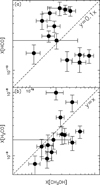 |
Fig. 4 Fractional abundance comparison. Panel a: comparison between the HCO and CH3OH fractional abundances derived from NCO(H2). The dashed line indicates the locus where y = 0.1x; Panel b: same as panel a but for H2CO and CH3OH. The dashed line indicates the locus where y = x. |
5.4 Abundance variations with Galactocentric distance
Figure 5 shows the CH3OH, HCO, and H2CO abundances against the source Galactocentric distances, RGC. Again, for HCO we show the results obtained using the excitation temperatures of CH3OH as Tex, which is more likely representative of a more extended envelope than that traced by H2CO. A simple linear regression fit to the data (solid line) shows an almost flat line, indicating that all abundances seem independent
of RGC. This suggests that the decreasing metallicity towards the external part of the Galaxy should not have an effect on the abundance of CH3OH. Bernal et al. (2021) came to the same conclusion. The main novel finding of the present study is that the abundances of HCO and H2CO, two progenitors of CH3OH, also do not decrease at metallicities lower than solar.
However, both abundance estimates are based on crucial assumptions: in the method of Blair et al. (2008), a CO-H2 conversion factor is assumed that is independent of RGC, while departures from a constant value are both observed and expected in both the Milky Way and external galaxies (Bolatto et al. 2013; Pineda et al. 2013; Casasola et al. 2017, 2020); in the method of Elia et al. (2021), a constant gas-to-dust ratio of 100 is assumed, which is also expected to change radially (e.g. Magrini et al. 2011). For the former, a Galactocentric trend has been proposed by Nakanishi & Sofue (2006, see their Eq. (2)), from which the CO-H2 conversion factor would vary by a factor of ~2 from 13 to 19 kpc, which is still consistent with an almost flat trend of the molecular abundances with RGC. For the latter, we investigated how the abundances change considering the Galactocentric increasing trend found by Giannetti et al. (2017) for the gas-to-dust ratio. In Fig. 5, we plot the abundances of CH3OH, HCO, and H2CO derived from NHer(H2) corrected according to Eq. (2) in Giannetti et al. (2017):
 (2)
(2)
where γ is the gas-to-dust ratio. We do not include the systematic uncertainties for simplicity. Please note that Eq. (2) assumes the same solar Galactocentric radius as we do.
As expected, now all molecules show abundances that decrease with RGC. However, this overall decrease does not seem to imply a reduced efficiency in the formation of these organic molecules, as we discuss in the following subsections.
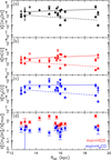 |
Fig. 5 Fractional abundances as a function of RGC. Panels a, b, and c: fractional abundances of, from top to bottom, CH3OH, HCO, and H2CO, as a function of RGC. The fractional abundances are derived from NCO(H2) given in Blair et al. (2008) (filled circles, Table 1) and from NHer(H2) given in Elia et al. (2021) (empty circles, Table 6). The stars correspond to the values computed from NHer(H2) corrected for the Galactocentric trend for the gas-to-dust ratio given in Giannetti et al. (2017). In all panels, the solid and dashed lines connect the values obtained at 13 and 19 kpc from a linear regression fit applied to the points computed from NHer(H2) without and with corrections, respectively, for the Galactocentric trend of the gas-to-dust ratio. Panel d: Abundance ratios X[CH3OH]/X[HCO] (red triangles) and X[CH3OH]/X[H2CO] (blue triangles) as a function of RGC. |
5.4.1 CH3OH
Let us begin by examining the case of CH3OH. A linear regression fit applied to the points plotted in panel a of Fig. 5 gives
![Mathematical equation: $X\left[ {{\rm{C}}{{\rm{H}}_{\rm{3}}}{\rm{OH}}} \right] = \left( { - 1.14 \times {{10}^{ - 10}}} \right) \times {R_{{\rm{GC}}}}\,{\rm{ + }}\,{\rm{2}}{\rm{.45}} \times {\rm{1}}{{\rm{0}}^{ - 9}}{\rm{,}}$](/articles/aa/full_html/2022/08/aa43532-22/aa43532-22-eq31.png) (3)
(3)
which implies that X[CH3OH] decreases by a factor of ~5 from 8.34 kpc (the Sun’s Galactocentric distance) to 19 kpc, extrapolating the trend found in the OG to the local Galaxy. According to the gradients given in Arellano-Córdova et al. (2020), the [O/H] and [C/H] ratios at 19 kpc are ~1.2 × 10⁻⁴ and ~4.7 × 10⁻⁵, that is approximately three and six times lower, respectively, than the values at the solar circle ([O/H] ~ 3 × 10⁻⁴ and [C/H] ~ 2.8 × 10⁻⁴). The more recent gradients given in Méndez-Delgado et al. (2022) provide [O/H] ~ 1.1 × 10⁻⁴ and [C/H] ~ 3.9 × 10⁻⁵, respectively, at 19 kpc, that is approximately three and seven times lower than solar ([O/H] ~ 3.1 × 10⁻⁴ and [C/H] ~ 2.6 × 10⁻⁴).
Therefore, the observed scaling factor of X[CH3OH] when applying the gas-to-dust ratio correction is consistent with that of the [C/H] ratio, or even marginally smaller than it. This suggests that the ‘efficiency’ in the formation of CH3OH, scaling with the availability of the parent element C, is at least as high as in the local Galaxy.
5.4.2 HCO and H2CO
Similarly, for X[HCO] and X[H2CO] we find a negligible decrease with RGC without considering the Galactocentric variation of the gas-to-dust ratio, and a decrease similar to that of CH3OH when applying it. More precisely, the linear regression fits to the points plotted in Fig. 5 provide
![Mathematical equation: $X\left[ {{\rm{HCO}}} \right] = \left( { - 1.38 \times {{10}^{ - 11}}} \right) \times {R_{{\rm{GC}}}}\,{\rm{ + }}\,{\rm{2}}{\rm{.95}} \times {\rm{1}}{{\rm{0}}^{ - 10}}{\rm{;}}$](/articles/aa/full_html/2022/08/aa43532-22/aa43532-22-eq32.png) (4)
(4)
![Mathematical equation: $X\left[ {{{\rm{H}}_2}{\rm{CO}}} \right] = \left( { - 1.18 \times {{10}^{ - 10}}} \right) \times {R_{{\rm{GC}}}}\,{\rm{ + }}\,{\rm{2}}{\rm{.51}} \times {\rm{1}}{{\rm{0}}^{ - 9}}{\rm{.}}$](/articles/aa/full_html/2022/08/aa43532-22/aa43532-22-eq33.png) (5)
(5)
These relations imply that both X[HCO] and X[H2CO] decrease by a factor ~5.5 from 8.34 kpc to 19 kpc. However, several caveats must be taken into consideration. First, the Galactocentric trend for the gas-to-dust ratio is associated with large systematic and statistical uncertainties (Giannetti et al. 2017), and local values may deviate significantly from the proposed trend. Second, our linear regression fit is obtained in the range RGC ~ 13–19 kpc and may not be appropriate down to RGC ~ 8.34 kpc. Third, the comparison with Galactocentric gradients needs to be taken with caution because the elemental abundances are still under debate. For example, the above-mentioned [C/H] decrease by a factor of six from the solar circle to 19 kpc found by Arellano-Córdova et al. (2020) is consistent with the 5.5 scaling factor predicted by Eqs. (4) and (5). However, the more recent gradients derived by Méndez-Delgado et al. (2022) indicate a scaling factor of ~7 for [C/H], which is marginally higher than our estimates.
Therefore, regardless of the above-mentioned uncertainties, we can conclude that the formation of these molecules is not inhibited in low-metallicity regimes, because all of them show abundances that are in line with the initial local abundances of the parent elements, and are very likely not lower than them. As discussed in Blair et al. (2008), Bernal et al. (2021), and in paper I, this finding, and the additional evidence that Earth-like planets are ubiquitously found in the Galaxy (Sect. 1), suggest that an appropriate ‘ground’ for the formation of habitable planets is also present in the OG, which means that a redefinition of the GHZ is needed that takes into account requirements other than metallicity.
5.4.3 Abundance ratios
Finally, the column density ratios N[CH3OH]/N[HCO] as a function of RGC are shown in the bottom panel of Fig. 5, and range from ~3 (19383+2711) to ~38 (WB89-621), with an average value of ~12 (median ~6.4). The ratios N[CH3OH]/N[H2CO] shown in the same plot are in between ~0.2 (WB89-399) and ~2.7 (WB89-437), with an average value of ~1.5 (median 1.4). The latter values are consistent with those measured by Bernal et al. (2021). Both ratios do not change with RGC, indicating once more that the chemistry that connects these species does not seem to vary (at least in an obvious way) with distance from the Galactic centre.
5.5 Methanol formation at low metallicity
The formation of CH3OH in dense star-forming cores is usually attributed in the most part to hydrogenation of CO, which on the surfaces of dust grains forms sequentially HCO, H2CO, CH2OH, and finally CH3OH. This is largely believed to be the most important formation route, given the inefficiency of gas phase routes at low temperatures (e.g. Garrod et al. 2006). If the main formation route is the same in the low-metallicity environment of the OG, the large abundances measured in this study would suggest an active surface chemistry followed by desorption mechanisms. In this respect, mantle evaporation either from internal protostellar activity or from external processes is typically invoked. Reactive desorption can also be important. As described by Vasyunin et al. (2017), reactive desorption becomes very efficient in regions where icy mantles become CO rich (i.e. in dense gas where the catastrophic CO freeze-out takes place and CO ice becomes the dominant component of the icy mantles). In paper I, we reported the detection of SiO J = 2–1 in 46% of the 35 targets. Among the 15 sources studied in this paper, 10 are clearly or tentatively associated with SiO emission, while five (WB89-789, WB89-006, WB89-076, WB89-080, and WB89-283) are not. On the other hand, all sources but 19383+2711 are associated with high-velocity wings in the HCO+ J = 1–0 line (paper I). This suggests that, even in the OG, the origin of CH3OH emission could be connected to evaporation of grain mantles caused by protostellar outflows. The non-detection of SiO in the five targets mentioned above may be due to insufficient sensitivity, given that these objects are among the least intense of the sample in the molecular lines analysed both in this paper (see Figs. A.1-A.5) and in paper I. However, first, the methanol line widths for all sources are narrow with respect to what is expected from material freshly released from outflows. Second, the full analysis of both SiO and HCO+ lines goes beyond the scope of this work and will be performed in a forthcoming paper (Fontani et al., in prep.). Moreover, this result could also be influenced by the source selection we performed in this study, and should be corroborated with a repeat analysis of greater statistical significance.
Chemical models with modified (lower) metallicities were developed in the past to interpret the formation of methanol and other COMs in the Magellanic Clouds as representatives of low-metallicity environments. Acharyya & Herbst (2015) modelled dense and cold clouds of the LMC and found that some observed results, especially for methanol, are better matched if these regions currently have lower temperatures. This is in agreement with the low temperature associated with our observed methanol emission. Moreover, Acharyya & Herbst (2016) modelled dense clouds of the SMC, in which the metallicity is lower than solar by a factor of 5, and found that for species that are fully (e.g. CH3OH) or partially produced on the grain surfaces (e.g. H2CO), the predicted abundances are not simply metallicity-scaled values but change in a more complex way. Our observations also indicate that care needs to be taken in the comparison with scaled-metallicity values, because different assumptions in the derivation of the abundances can lead to different conclusions (see Sect. 5.4).
Pauly & Garrod (2018) used the gas-grain chemical model MAGICKAL to model the chemistry in sources of the Magellanic Clouds where massive young stellar objects are forming. These authors discuss the formation and evolution of several species chemically connected to CH3OH, and of CH3OH itself, and conclude that the methanol abundance is even found to be enhanced in low-metallicity environments. In fact, their models predict that the amount of CH3OH with respect to CO increases as the elemental C decreases, which indicates a more efficient abundance at lower metallicities. This effect could be due to the smaller C/O ratio (see Sect. 5.4), meaning that the bulk of C is in the form of CO, which is required to form CH3OH. If confirmed, this would imply a lower abundance of carbon chains, or other carbon-rich molecules. The exploitation of the detected carbon-rich species listed in paper I, among which c-C3H2, C4H, and CCS are found, will be performed in forthcoming papers (Fontani et al., in prep.).
However, when modelling the chemistry, several ingredients need to be considered and many crucial ones could vary significantly with Galactocentric radius. For example, as also discussed by Viti et al. (2020) for example, the abundances of molecules containing carbon in external galaxies known to be associated with different visual extinctions, cosmic-ray ionisation rates, and/or ultraviolet (UV) radiation fields are predicted to change by orders of magnitude. Because these parameters are expected to vary within the Milky Way as well (e.g. both the interstellar UV field and the cosmic-ray ionisation rate are expected to be lower in the OG due to lower numbers of massive stars and supernovae explosions), a thorough analysis of the variations with RGC of all these key parameters is absolutely needed in order to appropriately model the chemistry. This discussion is particularly urgent because important complex species in external galaxies are now detected easily thanks to the powerful (sub)millimetre telescopes now available (see e.g. the first results of the ALCHEMI ALMA large program; Martín et al. 2021), showing that a rich chemistry can develop even in external galaxies. This goes beyond the scope of this paper, but strongly calls for both observational works to measure and constrain these parameters as a function of the Galactocentric radius, and theoretical works aimed at identifying the physical conditions that mostly affect the chemistry in such modified environments. In particular, chemical evolution models (e.g. Romano et al. 2020) could be used in the future to estimate the amount and density of massive stars – which are important sources of both UV photons and cosmic rays – as a function of Galactocentric radius.
6 Conclusions
We detected CH3OH, HCO, and H2CO emission associated with 15 star-forming regions of the outer Galaxy. Derived angular diameters, excitation temperatures, and line widths of CH3OH indicate that the emission is dominated by a cold and quiescent gaseous envelope. The CH3OH fractional abundances are in the range ~0.6–7.4 × 10⁻⁹. These values are consistent with those found for similar star-forming regions in the local and inner Galaxy. We find that some CH3OH line parameters, such as centroid velocity, FWHM, and (less obviously) fractional abundance with respect to H2, are correlated with those of H2CO, while they do not appear correlated with those of HCO. This may indicate that hydrogenation of CH3OH from iced H2CO, followed by evaporation or other desorption mechanisms from grain mantles, could also be a relevant source of CH3OH in the OG. On the other hand, the HCO emission we observe can also be significantly produced in the gas phase from routes not involving H2CO or Ch3OH. However, in these observations, the CH3OH emission is clearly associated with an extended and relatively quiescent envelope rather than with shocked or sputtered material, and therefore this conclusion needs to be corroborated by higher angular resolution observations. The total column densities and fractional abundances with respect to H2 indicate that the production of CH3OH is not inhibited even at Galactocentric distances of ~19 kpc, where the carbon abundance is estimated to be lower than solar by a factor of ~6–7. Moreover, even considering corrections to the estimated abundances taking the variations of the gas-to-dust ratio with RGC into account, our abundances are in line with metallicity-scaled values. The high abundance of CH3OH at large RGC could be due to the smaller C/O ratio at these large Galactocentric distances, which implies that the bulk of C is in the form of CO, which is required to form CH3OH. Our results confirm that organic chemistry is active and efficient even in the outermost star-forming regions of the Milky Way, and support the idea that the outer boundaries of the Galactic habitable zone need to be re-discussed in light of the capacity of the interstellar medium to form organic molecules even at such low metallicities.
Acknowledgements
We thank the anonymous referee for their valuable and constructive comments. F.F. is grateful to the IRAM 30 m staff for their precious help during the observations. L.C. has received partial support from the Spanish State Research Agency (AEI; project number PID2019-105552RB-C41). V.M.R. acknowledges support from the Comunidad de Madrid through the Atracción de Talento Investigador Modalidad 1 (Doctores con experiencia) Grant (COOL: Cosmic Origins of Life; 2019-T1/TIC-15379). The research leading to these results has received funding from the European Union’s Horizon 2020 research and innovation programme under grant agreement nos. 730562 and 101004719 (ORP/https://www.orp-h2020.eu).
Appendix A Spectra
This Appendix shows the spectra of CH3OH, HCO, and H2CO analysed in this work (see Sect. 2).
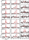 |
Fig. A.1 Spectra of CH3OH lines. The lines are identified in the 3 and 2 mm bands (Table 2) of the IRAM-30m telescope towards the first eight sources listed in Table 1. The red curve in each frame represents the best fit to the lines performed with madcuba (see Sect. 3). |
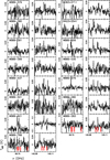 |
Fig. A.3 Residuals obtained from the best fits shown in Figs. A.1 and A.2. At 2 mm, we only show the residuals of the lines shown in the second panel of Figs A.1 and A.2. The frequency of the fitted lines are indicated by vertical red lines. |
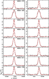 |
Fig. A.4 Spectra of H2CO lines. The lines, listed in Table 2, are observed at 2 mm with the IRAM-30m telescope towards the first eight sources listed in Table 1. The red curve in each frame represents the best fit to the lines performed with madcuba (see Sect. 3). |
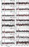 |
Fig. A.6 Spectra of HCO lines. The lines, listed in Table 2, are observed at 3 mm with the IRAM-30m telescope towards the first eight sources listed in Table 1. The red curve in each frame represents the best fit to the lines performed with madcuba by fixing Tex at the excitation temperature of CH3OH (see Sects. 3 and 4.3). |
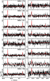 |
Fig. A.8 Same as Fig. A.6, with the best fit obtained with madcuba fixing Tex at the excitation temperature of H2CO (see Sects. 3 and 4.3). |
Appendix B Results of HCO line fitting assuming Tex from H2CO
Fit results to the HCO lines obtained with madcuba fixing Tex at the excitation temperature of H2CO (see Sects. 3 and 4.3).
HCO line parameters.
References
- Acharyya, K., & Herbst, E. 2015, ApJ, 812, 142A [NASA ADS] [CrossRef] [Google Scholar]
- Acharyya, K., & Herbst, E. 2016, ApJ, 822, 105A [NASA ADS] [CrossRef] [Google Scholar]
- Arellano-Córdova, K. Z., Esteban, C., García-Rojas, J., & Méndez-Delgado, J. E. 2020, MNRAS, 496, 1051 [Google Scholar]
- Bacmann, A., & Faure, A. 2016, A&A, 587, A130 [NASA ADS] [CrossRef] [EDP Sciences] [Google Scholar]
- Bennett, C. J., & Kaiser, R. I., 2007, ApJ, 661, 899 [Google Scholar]
- Bernal, J. J., Sephus, C. D., & Ziurys, L. M. 2021, ApJ, 922, 106 [NASA ADS] [CrossRef] [Google Scholar]
- Blair, S. K., Magnani, L., Brand, J., & Wouterloot, J. G. A. 2008, AsBio, 8, 59 [NASA ADS] [Google Scholar]
- Bolatto, A. D., Wolfire, M., Leroy, A. K. 2013, ARA&A, 51, 207 [CrossRef] [Google Scholar]
- Buchhave, L. A., Latham, D. W., Johansen, A., et al. 2012, Nature, 486, 375 [NASA ADS] [Google Scholar]
- Casasola, V., Cassarà, L. P., Bianchi, S., et al. 2017, A&A, 605, A18 [NASA ADS] [CrossRef] [EDP Sciences] [Google Scholar]
- Casasola, V., Bianchi, S., De Vis, P., et al. 2020, A&A, 633, A100 [NASA ADS] [CrossRef] [EDP Sciences] [Google Scholar]
- Chacón-Tanarro, A., Caselli, P., Bizzocchi, L., et al. 2019, A&A, 622, A141 [Google Scholar]
- Charnley, S. B., Tielens, A. G. G. M., & Millar, T. J. 1992, ApJL, 399, L71 [NASA ADS] [CrossRef] [Google Scholar]
- Chen, Y.-J., Ciaravella, A., Muñoz Caro, G. M., et al. 2013, ApJ, 778, 162 [NASA ADS] [CrossRef] [Google Scholar]
- Chuang, K.-J., Fedoseev, G., Qasim, D., et al. 2016, MNRAS, 467, 2552 [NASA ADS] [Google Scholar]
- Dai, Y.-Z., Liu, H.-G., An, D.-S., & Zhou, J.-L. 2021, AJ, 162, 46 [NASA ADS] [CrossRef] [Google Scholar]
- Dartois, E., Demyk, K., d’Hendecourt, L., & Ehrenfreund, P., 1999, A&A, 351, 1066 [NASA ADS] [Google Scholar]
- Digel, S., de Geus, E., Thaddeus, P. 1994, ApJ, 422, 92 [NASA ADS] [CrossRef] [Google Scholar]
- Elia, D., Merello, M., Molinari, S., et al. 2021, MNRAS, 504, 2742 [NASA ADS] [CrossRef] [Google Scholar]
- Endres, P., Schlemmer, S., Schilke, P., Stutzki, J., & Müller, H. S. P. 2016, J. Mol. Spectro., 327, 95 [NASA ADS] [CrossRef] [Google Scholar]
- Esteban, C., Fang, X., & García-Rojas, J., Toribio San Cipriano, L. 2017, MNRAS, 471, 987 [NASA ADS] [CrossRef] [Google Scholar]
- Fedoseev, G., Chuang, K.-J., van Dishoeck, E. F., Ioppolo, S., & Linnartz, H. 2016, MNRAS, 460, 4297 [NASA ADS] [CrossRef] [Google Scholar]
- Fontani, F., Cesaroni, R., Caselli, P., & Olmi, L. 2002, A&A, 389, 603 [NASA ADS] [CrossRef] [EDP Sciences] [Google Scholar]
- Fontani, F., Colzi, L., Bizzocchi, L., et al. 2022 A&A, 660, A76 [NASA ADS] [CrossRef] [EDP Sciences] [Google Scholar]
- Garrod, R., Park, I. H., Caselli, P., & Herbst, E. 2006, FaDi, 133 51 [NASA ADS] [Google Scholar]
- Gerner, T., Beuther, H., Semenov, D., et al. 2014, A&A, 563, A97 [NASA ADS] [CrossRef] [EDP Sciences] [Google Scholar]
- Giannetti, A., Leurini, S., König, S., et al. 2017, A&A, 606, L12 [NASA ADS] [CrossRef] [EDP Sciences] [Google Scholar]
- Hickson, K. M., Loison, J.-C., Nunez-Reyes, D., Mereau, R., 2016, ArXiv eprints, [arXiv:1608.08877] [Google Scholar]
- Kovtyukh, V., Lemasle, B., Bono, G., et al. 2022, MNRAS, 510, 1894 [Google Scholar]
- Kutner, M. L., & Ulich, B. L. 1981, ApJ, 250, 341 [NASA ADS] [CrossRef] [Google Scholar]
- Magrini, L., Bianchi, S., Corbelli, E., et al. 2011, A&A, 535, A13 [NASA ADS] [CrossRef] [EDP Sciences] [Google Scholar]
- Maliuk, A., & Budaj, J. 2020, A&A, 635, A191 [NASA ADS] [CrossRef] [EDP Sciences] [Google Scholar]
- Martín, S., Martín-Pintado, J., Blanco-Sánchez, C., et al. 2019, A&A, 631, A159 [Google Scholar]
- Martín, S., Mangum, J. G., Harada, N., et al. 2021, A&A, 656, A46 [NASA ADS] [CrossRef] [EDP Sciences] [Google Scholar]
- Méndez-Delgado, J. E., Amayo, A., Arellano-Córdova, K. Z., et al. 2022, MNRAS, 510, 4436 [CrossRef] [Google Scholar]
- Minier, V., & Booth, R. S. 2002, A&A, 387, 179 [NASA ADS] [CrossRef] [EDP Sciences] [Google Scholar]
- Nakanishi, H., & Sofue, Y. 2006, PASJ, 58, 847 [NASA ADS] [Google Scholar]
- Öberg, K. I., Garrod, R. T., van Dishoeck, E. F., & Linnartz, H. 2009, A&A, 504, 891 [NASA ADS] [CrossRef] [EDP Sciences] [Google Scholar]
- Pauly, T., & Garrod, R. T. 2018, ApJ, 854, 13 [NASA ADS] [CrossRef] [Google Scholar]
- Pickett, H. M., Poynter, R. L., Cohen, E. A., et al. 1998, J. Quant. Spectr. Rad. Transf., 60, 883 [Google Scholar]
- Pineda, J. L., Langer, W. D., Velusamy, T., & Goldsmith, P. F. 2013, A&A, 554, A103 [CrossRef] [EDP Sciences] [Google Scholar]
- Prantzos, N. 2008, Space Sci. Rev., 135, 313 [NASA ADS] [CrossRef] [Google Scholar]
- Ramírez, I., Asplund, M., Baumann, P., Meléndez, J., & Bensby, T. 2010, A&A, 521, A33 [Google Scholar]
- Reid, M. J., Menten, K. M., Brunthaler, A., et al. 2014, ApJ, 783, 130 [Google Scholar]
- Rivilla, V. M., Beltrán, M. T., Cesaroni, R., et al. 2017, A&A, 598, A59 [NASA ADS] [CrossRef] [EDP Sciences] [Google Scholar]
- Rivilla, V. M., Beltrán, M. T., Vasyunin, A., et al. 2019, MNRAS, 483, 806 [NASA ADS] [CrossRef] [Google Scholar]
- Romano, D., Franchini, M., Grisoni, V., et al. 2020, A&A, 639, A37 [NASA ADS] [CrossRef] [EDP Sciences] [Google Scholar]
- Sewiło, M., Indebetouw, R., Charnley, S. B., et al. 2018, ApJL, 853, L19 [CrossRef] [Google Scholar]
- Sewiło, M., Cordiner, M., Charnley, S. B., et al. 2022, ApJ, 931, 102 [CrossRef] [Google Scholar]
- Shimonishi, T., Watanabe, Y., Nishimura, Y., et al. 2018, ApJ, 891, 164 [Google Scholar]
- Shimonishi, T., Izumi, N. Furuya, K., & Yasui, C. 2021, ApJ, 922, 206 [NASA ADS] [CrossRef] [Google Scholar]
- Shirley, Y. L. 2015, PASP, 127, 299 [Google Scholar]
- Spina, L., Magrini, L., & Cunha, K. 2022, Universe, 8, 87S [NASA ADS] [CrossRef] [Google Scholar]
- Spitoni, E., Matteucci, F., & Sozzetti, A. 2014, MNRAS, 440, 2588 [NASA ADS] [CrossRef] [Google Scholar]
- Spitoni, E., Gioannini, L., & Matteucci, F. 2017, A&A, 605, A38 [NASA ADS] [CrossRef] [EDP Sciences] [Google Scholar]
- Tielens, A. G. G. M., & Hagen, W., 1982, A&A, 114, 245 [Google Scholar]
- van der Tak, F. F. S., van Dishoeck, E. F., & Caselli, P. 2000, A&A, 361, 327 [NASA ADS] [Google Scholar]
- Vasyunina, T., Vasyunin, A. I., Herbst, E., et al. 2014, ApJ, 780, 85 [Google Scholar]
- Vasyunin, A. I., Caselli, P., Dulieu, F., & Jiménez-Serra, I. 2017, ApJ, 842, 33 [Google Scholar]
- Viti, S., Fontani, F., & Jiménez-Serra, I. 2020, MNRAS, 497, 4333 [NASA ADS] [CrossRef] [Google Scholar]
- Watanabe, N., & Kouchi, A. 2002, ApJ, 571, L173 [Google Scholar]
- Wenger, T. V., Balser, D. S., Anderson, L. D., & Bania, T. M. 2019, ApJ, 887, 114 [NASA ADS] [CrossRef] [Google Scholar]
- Woods, P. M., Kelly, G., Viti, S., et al. 2012, ApJ, 750, 19 [NASA ADS] [CrossRef] [Google Scholar]
- Woods, P. M., Slater, B., Raza, Z., et al. 2013, ApJ, 777, 90 [Google Scholar]
madcuba is a software developed in the Madrid Center of Astrobiology (INTA-CSIC) which enables to visualise and analyse single spectra and data cubes: https://cab.inta-csic.es/madcuba/
All Tables
Abundances of CH3OH calculated in this work, and towards other star-forming regions both in the Galaxy and in external galaxies.
All Figures
|
Fig. 1 Comparison between linear diameters obtained for CH3OH (x-axis) and H2CO (y-axis). Both diameters are calculated from the angular diameters given in Tables 3 and 4, respectively, and the source heliocentric distances in Table 1. The dashed line is the locus where D[CH3OH] = D[H2CO]. |
| In the text | |
|
Fig. 2 Tex and FWHM comparison for CH3OH, H2CO, and HCO. Top panel: comparison between the best-fit Tex estimated from H2CO and CH3OH. The dotted line indicates Tex[H2CO] = Tex[CH3OH]. Middle and bottom panels: Tex against FWHM measured from H2CO (middle) and from CH3OH (bottom). The CH3OH and H2CO parameters are given in Tables 3 and 4, respectively. |
| In the text | |
|
Fig. 3 Velocity and FWHM comparison for CH3OH, H2CO, and HCO. Top panel: velocity difference between H2CO and CH3OH versus the difference between HCO and CH3OH. Middle and bottom panels: comparison between the FWHM measured for HCO and CH3OH (middle) and that measured from CH3OH and H2CO (bottom). The dotted line indicates FWHM[HCO] = FWHM[CH3OH] or FWHM[H2CO] = FWHM[CH3OH]. The HCO data for 19383+2711 is missing from all panels, for which the resulting fit parameters are affected by the unresolved second velocity feature (see Sect. 4.3). |
| In the text | |
|
Fig. 4 Fractional abundance comparison. Panel a: comparison between the HCO and CH3OH fractional abundances derived from NCO(H2). The dashed line indicates the locus where y = 0.1x; Panel b: same as panel a but for H2CO and CH3OH. The dashed line indicates the locus where y = x. |
| In the text | |
|
Fig. 5 Fractional abundances as a function of RGC. Panels a, b, and c: fractional abundances of, from top to bottom, CH3OH, HCO, and H2CO, as a function of RGC. The fractional abundances are derived from NCO(H2) given in Blair et al. (2008) (filled circles, Table 1) and from NHer(H2) given in Elia et al. (2021) (empty circles, Table 6). The stars correspond to the values computed from NHer(H2) corrected for the Galactocentric trend for the gas-to-dust ratio given in Giannetti et al. (2017). In all panels, the solid and dashed lines connect the values obtained at 13 and 19 kpc from a linear regression fit applied to the points computed from NHer(H2) without and with corrections, respectively, for the Galactocentric trend of the gas-to-dust ratio. Panel d: Abundance ratios X[CH3OH]/X[HCO] (red triangles) and X[CH3OH]/X[H2CO] (blue triangles) as a function of RGC. |
| In the text | |
|
Fig. A.1 Spectra of CH3OH lines. The lines are identified in the 3 and 2 mm bands (Table 2) of the IRAM-30m telescope towards the first eight sources listed in Table 1. The red curve in each frame represents the best fit to the lines performed with madcuba (see Sect. 3). |
| In the text | |
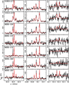 |
Fig. A.2 Same as Fig A.1 for the remaining seven sources. |
| In the text | |
|
Fig. A.3 Residuals obtained from the best fits shown in Figs. A.1 and A.2. At 2 mm, we only show the residuals of the lines shown in the second panel of Figs A.1 and A.2. The frequency of the fitted lines are indicated by vertical red lines. |
| In the text | |
|
Fig. A.4 Spectra of H2CO lines. The lines, listed in Table 2, are observed at 2 mm with the IRAM-30m telescope towards the first eight sources listed in Table 1. The red curve in each frame represents the best fit to the lines performed with madcuba (see Sect. 3). |
| In the text | |
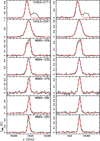 |
Fig. A.5 Same as Fig A.4 for the remaining seven sources. |
| In the text | |
|
Fig. A.6 Spectra of HCO lines. The lines, listed in Table 2, are observed at 3 mm with the IRAM-30m telescope towards the first eight sources listed in Table 1. The red curve in each frame represents the best fit to the lines performed with madcuba by fixing Tex at the excitation temperature of CH3OH (see Sects. 3 and 4.3). |
| In the text | |
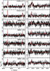 |
Fig. A.7 Same as Fig A.6 for the remaining seven sources. |
| In the text | |
|
Fig. A.8 Same as Fig. A.6, with the best fit obtained with madcuba fixing Tex at the excitation temperature of H2CO (see Sects. 3 and 4.3). |
| In the text | |
 |
Fig. A.9 Same as Fig A.8 for the remaining seven sources. |
| In the text | |
Current usage metrics show cumulative count of Article Views (full-text article views including HTML views, PDF and ePub downloads, according to the available data) and Abstracts Views on Vision4Press platform.
Data correspond to usage on the plateform after 2015. The current usage metrics is available 48-96 hours after online publication and is updated daily on week days.
Initial download of the metrics may take a while.