| Issue |
A&A
Volume 691, November 2024
|
|
|---|---|---|
| Article Number | A180 | |
| Number of page(s) | 15 | |
| Section | Interstellar and circumstellar matter | |
| DOI | https://doi.org/10.1051/0004-6361/202451500 | |
| Published online | 11 November 2024 | |
CHEMOUT: CHEMical complexity in star-forming regions of the OUTer Galaxy
IV. ALMA observations of organic species at a galactocentric radius of ~23 kpc
1
INAF – Osservatorio Astrofisico di Arcetri,
Largo E. Fermi 5,
50125
Florence,
Italy
2
Max-Planck-Institut für extraterrestrische Physik,
Giessenbachstraße 1,
85748
Garching bei München,
Germany
3
LERMA, Observatoire de Paris, PSL Research University, CNRS, Sorbonne Université,
92190
Meudon,
France
4
Leiden Observatory, Leiden University,
PO Box 9513,
2300 RA
Leiden,
The Netherlands
5
Dipartimento di Fisica e Astronomia, Università di Firenze,
Via G. Sansone 1,
50019
Sesto Fiorentino, Firenze,
Italy
6
Centro de Astrobiología (CSIC-INTA),
Ctra Ajalvir km 4,
28850, Torrejón de Ardoz,
Madrid,
Spain
7
Institut de Ciències de l’Espai (ICE, CSIC),
Campus UAB, Carrer de Can Magrans s/n,
08193
Bellaterra (Barcelona),
Spain
8
Institut d’Estudis Espacials de Catalunya (IEEC),
08860
Castelldefels (Barcelona),
Spain
★ Corresponding author; This email address is being protected from spambots. You need JavaScript enabled to view it.
Received:
14
July
2024
Accepted:
30
September
2024
Abstract
Context. Single-dish observations suggest that the abundances of organic species in star-forming regions of the outer Galaxy, which are characterised by sub-solar metallicities, are comparable to those found in the local Galaxy.
Aims. To understand this counter-intuitive result and avoid a misleading interpretation due to beam dilution effects at these large distances, spatially resolved molecular emission maps are needed to correctly link the measured abundances and local physical properties.
Methods. We observed several organic molecules with the Atacama Large Millimeter Array towards WB89-671, the source with the largest galactocentric distance (23.4 kpc) of the project CHEMical complexity in star-forming regions of the OUTer Galaxy (CHEMOUT) at a resolution of ~15 000 au. We compared the observed molecular abundances with chemical model predictions.
Results. We detected emission of c-C3H2, C4H, CH3OH, H2CO, HCO, H13CO+, HCS+, CS, HN13C, and SO. The emission morphology is complex, extended, and different in each tracer. In particular, the most intense emission in H13CO+, H2CO and c-C3H2 arises from two millimeter-continuum infrared-bright cores. The most intense CH3OH and SO emission predominantly arises from the part of the filament that lacks continuum sources. The narrow line widths across the filament indicate quiescent gas in spite of the two embedded protostars. The derived molecular column densities are comparable with those in local star-forming regions, and they suggest an anti-correlation between hydrocarbons, ions, HCO, and H2CO on the one hand, and CH3OH and SO on the other.
Conclusions. The static chemical models that match the observed column densities best favour low-energy conditions that are expected at large galactocentric radii, but they also favour carbon elemental abundances that exceed those derived by extrapolating the [C/H] galactocentric gradient at 23 kpc by three times. This would indicate a flatter [C/H] trend at large galactocentric radii, which is in line with a flat abundance of organics. However, to properly reproduce the chemical composition of each region, models should include dynamical evolution.
Key words: stars: formation / ISM: molecules
© The Authors 2024
 Open Access article, published by EDP Sciences, under the terms of the Creative Commons Attribution License (https://creativecommons.org/licenses/by/4.0), which permits unrestricted use, distribution, and reproduction in any medium, provided the original work is properly cited.
This article is published in open access under the Subscribe to Open model. This email address is being protected from spambots. You need JavaScript enabled to view it. to support open access publication.
1 Introduction
The outer Galaxy (OG), that is, the part of the Milky Way that extends beyond the solar circle to the outermost edge of the Galactic disc (~27 kpc; López-Corredoira et al. 2018), was thought to be an environment that is not optimal for the formation of molecules and planetesimals. The reason is its sub-solar metallicity, that is, the low abundance of elements heavier than helium. In particular, the elemental abundances of oxygen, carbon, and nitrogen, that is, the three most abundant elements in the Universe after hydrogen and helium, and the most important biogenic elements, decrease as a function of the galactocentric distance, RGC (Esteban et al. 2017; Arellano-Córdova et al. 2020; Méndez-Delgado et al. 2022). For example, the fractional abundance of oxygen relative to hydrogen, [O/H], gradually decreases from the inner Galaxy to the OG and reaches about one-fifth of the solar value at about 20 kpc (see e.g. Esteban et al. 2017; Méndez-Delgado et al. 2022). For carbon, the decrease in the [C/H] ratio is even more pronounced. It reaches about one-seventh to one-eigth of the solar value at ~20 kpc (Arellano-Córdova et al. 2020; Méndez-Delgado et al. 2022). These low abundances of heavy elements in the OG previously suggested that this zone was not suitable for forming planetary systems in which Earth-like planets could be born and might be capable of sustaining life (Ramírez et al. 2010). For this reason, the OG was excluded from the so-called Galactic habitable zone (GHZ), which is the portion of the Milky Way with the highest chance of forming and developing complex forms of life on (exo-)planets (Gonzalez et al. 2001). Because of this, its chemical complexity has been little explored so far.
However, it is being discovered that the presence of small, terrestrial planets is independent of the galactocentric distance (e.g. Buchhave et al. 2012; Maliuk & Budaj 2020), and that molecules, including complex organic molecules (COMs; organic species with six or more atoms), are found to be more abundant than expected in star-forming regions with a metal- licity lower than solar, both in the OG (e.g. Blair et al. 2008; Shimonishi et al. 2021; Bernal et al. 2021; Fontani et al. 2022a) and in external galaxies (e.g. Shimonishi et al. 2018; Sewiło et al. 2018). However, molecular formation processes could be different from those in the inner or local Galaxy due to the difference in the metallicity and other environmental conditions. For example, UV irradiation from high-mass stars should be lower in the OG on average due to the lower concentration of high-mass stars. Therefore, the abundances of species sensitive to this parameter might also be affected by this environmental change. It is thus crucial to observe molecules in star-forming regions of the OG to constrain models that are adapted to these sub-solar metallicity environments.
The few studies performed so far in the OG mentioned above only provided abundances of a limited number of abundant species, and hence they can answer only partial questions. Blair et al. (2008), Bernal et al. (2021), and Fontani et al. (2022b) detected formaldehyde (H2 CO) and methanol (CH3 OH) in starforming regions of the OG up to 24 kpc. H2CO is an important precursor of CH3OH, the simplest complex organics, because its formation in cold star-forming cores proceeds on the surface of dust grains via successive hydrogenation of CO (HCO → H2CO → CH3O/CH2OH → CH3OH, e.g. Pauly & Garrod 2018). However, H2CO can also form in the gas-phase, unlike CH3OH, in regions where a significant fraction of C is not yet locked into CO (Ramal-Olmedo et al. 2021). If this is so, H2CO should form together with species such as carbon chains, which also need a large amount of C that is not locked in CO. This implies that in regions where the C/O ratio is lower, most of the C should be in the form of CO, and carbon chains should have a lower abundance than CH3OH. The OG is an environment that should have this property, because the [C/H] decrease with RGC is steeper than that of [O/H] (Arellano-Córdova et al. 2020; Méndez-Delgado et al. 2022). The opposite is expected in the inner Galaxy. On the other hand, a dust extinction that is lower in the OG than in the local Galaxy would imply an easier dissociation of CO in the gas phase, favouring the formation of carbon chains. This example shows that the formation of even a relatively simple organic molecule such as H2CO, and its relation with CH3OH, can be different in the outer and inner Galaxy.
The project CHEMical complexity of star-forming regions in the OUTer Galaxy (CHEMOUT; Fontani et al. 2022a,b; Colzi et al. 2022) studies the formation of molecules in the outer Galaxy based on observations of 35 molecular cloud cores associated with star-forming regions in which RGC is in between 9 and 23 kpc. Using the Institut de Radioastronomie Millimétrique (IRAM) 30m telescope, we detected several simple and complex carbon-bearing molecules including organics (c-C3H2, HCO+, H13CO+, HCO, C4H, HCS+, HCN, CH3CCH). Inorganic tracers of star formation activity (SO, SiO, and N2D+) were detected as well. The detection of all these species is expected to constrain their formation or destruction pathways better and to highlight similarities and differences with those known to be efficient in the local and inner Galaxy, where the C/O ratio is different. However, the results of Blair et al. (2008), Bernal et al. (2021), and Fontani et al. (2022a,b) were based on observations of single-dish telescopes, and they thus only provide abundances averaged over the angular scales of their main beams (~27−63″). At the distance of the CHEMOUT targets, that is, 8–15 kpc from the Sun (Fontani et al. 2022a), an angular scale of 27″ corresponds to 1–2 pc, or 200 000–400 000 au, which is larger than the typical linear scale of a single star-forming core (0.05–0.1 pc) by at least a factor of 10.
In this work, we present high-angular resolution images obtained with the Atacama Large Millimeter Array (ALMA) to resolve the molecular emission towards the source WB89- 670 (IRAS 05343+3605 Wouterloot & Brand 1989), WB670 hereafter. The source is located at an RGC of ~23.4 kpc (heliocentric distance ~15.1 kpc, Fontani et al. 2022a), in the direction of the Galactic anticentre (Galactic coordinates Lon.=173.014°, Lat.=2.38°). This CHEMOUT target lies at the largest galac- tocentric distance and is thus associated with the lowest environmental [C/H] and [O/H] of the sample and also with the lowest C/O ratio (Esteban et al. 2017; Arellano-Córdova et al. 2020; Méndez-Delgado et al. 2022). When we extrapolate the elemental galactocentric gradients of carbon and oxygen measured by Méndez-Delgado et al. (2022) to 23.4 kpc, the fractional abundances [C/H] and [O/H] are 1.8× 10⁻⁵ and 6.7×10⁻⁵, respectively. Considering the solar values of [C/H] ~ 2.6 × 10⁻⁴ and [O/H] ~ 3.1 × 10⁻⁴, the [C/O] ratio should be ~3.1 times lower than solar in the natal cloud of WB670. The source harbours near- and mid-infrared sources detected in the images of the Two Micron All-Sky Survey (2MASS, Cutri et al. 2003) and the Wide-field Infrared Survey Explorer (WISE, Wright et al. 2010, Fig. 1), which are associated with molecular gas where rotational transitions of c-C3H2, C4H, CCS, H13CO+, HCO+, and HCN (Fontani et al. 2022a), CH3OH (Bernal et al. 2021), and H2CO (Blair et al. 2008) were detected. No COMs except for CH3OH were identified in this source. The narrow width at half maximum (about 1 km s−1) in the line profile of HCO+J = 1–0 suggests that the bulk emission in this transition is from quiescent material, but the simultaneous detection of non-Gaussian wings at high velocities also indicates embedded protostellar activity (Fontani et al. 2022a).
The paper is organised as follows: The observations and the data reduction are described in Sect. 2. The observational results are shown in Sect. 3. The spectral analysis and derivation of the molecular column densities is illustrated in Sect. 4. A discussion of the results and a comparison with chemical modelling is provided in Sect. 5. Our conclusions and future perspectives are given in Sect. 6.
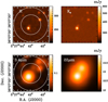 |
Fig. 1 Near- and mid-infrared images of WB89-670. The panels in the top row show the images at 1.25 µm (H) and 2.15 µm (Ks) from the 2MASS survey. The panels in the bottom row show the WISE images at the wavelengths indicated in the top left corner. The white circles are the ALMA primary beams at ~86 GHz and ~150 GHz, which are 66″ (i.e. ~7.5 pc) and 38″ (i.e. ~4.3 pc), respectively. |
Spectral setup and observational parameters.
2 Observations and data reduction
The observations were carried out with ALMA during Cycle 9 on three dates: December 27, 2022, using 45 antennas, and January 8 and 9, 2023 (project 2022.1.00911.S, P.I.: F. Fontani), using 41 antennas. The phase centre was set to the equatorial coordinates R.A.(J2000)=05h37m41.9s and Dec(J2000)=36°07′22″. The local standard of rest velocity is −17.4 km s−1 (Fontani et al. 2022a). We observed several spectral windows in bands 3 and 4. Information about their central frequencies, spectral resolution, and sensitivity is given in Table 1. For all the spectral windows, the sources we used as flux and bandpass calibrators were J0423–0120 in band 3 and J0854+2006 in band 4, and J0547+2721 and J0550+2326 were used as gain (amplitude and phase) calibrators. The uncertainties in the flux calibration are ~5%. The primary beam (i.e. the full width at half maximum, FWHM, of the main beam of a 12m antenna) ranges from ~67″ at 84.5 GHz to ~57″ at 99.3 GHz, and from ~41″ at 140 GHz to ~37″ at 153.5 GHz.
The calibrated data were produced by the calibration pipeline of the Common Astronomy Software Applications (CASA; McMullin et al. 2007). The pipeline version we used was casapipe-6.4.1. Imaging and deconvolution were then performed on the calibrated uv tables with the GILDAS1 software after conversion of the calibrated uv tables from measurement sets in uvfits format and then in GILDAS format. To be sensitive to the source extension, the clean maps were created using natural weighting. As significant emission is detected at the edge of the primary beam, we analysed the images corrected for the primary beam. We attempted to perform self-calibration, but the selfcalibrated images showed no significant improvement because the continuum emission is faint, and hence we analysed the nonself-calibrated images. In the channel maps, the root mean square (rms) varies between 1.8 and 3.9 mJy beam−1 in band 3 and between 8.8 and 18 mJy beam−1 in band 4. In the continuum images, the rms is ~0.025 mJy beam−1 in band 3 and ~0.1 mJy beam−1 in band 4. The angular resolution in both ALMA bands is ~1.4−1.5″, corresponding to ~0.1 pc, or ~20000 au. In all the images, the maximum recoverable scale is ~20″. The detected molecular lines and their spectroscopic parameters are listed in Table 2.
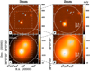 |
Fig. 2 Continuum emission detected towards WB89-670 with ALMA. The light blue contours in the left and right panels correspond to the 3 mm and 2 mm continuum emission, respectively. Contours start from the 3σ rms level (~8 × 10⁻⁵ Jy at 3 mm and ~3 × 10⁻⁴ Jy at 2 mm), and are in steps of ~5 × 10⁻⁵ Jy and ~2 × 10⁻⁴ Jy, respectively. The synthesised beam is depicted in the bottom left corner, and the white circle indicates the ALMA primary beam at the two wavelengths. The region shown in the 2 mm images corresponds to the dashed square illustrated in the top left panel. The heat-colour image in background is the Ks band of 2MASS (Fig. 1) in the top panels and the WISE 22µm band in the bottom panels. |
3 Analysis of the maps
3.1 Millimeter-continuum emission
The millimeter-continuum emission detected towards WB670 in both ALMA bands is shown in Fig. 2. Two compact sources are detected. The strongest source, which we call N, is detected in the 3 mm image with a signal-to-noise ratio of 14 (peak flux density ~3.5 × 10⁻⁴ Jy). Core N is undetected or barely detected in the near-infrared, and it is clearly detected in the mid-infrared. The other source, called S, coincides with the main infrared source detected in all 2MASS and WISE images, and it is detected in the 3 mm image with a signal-to-noise ratio of 7 (peak flux density ~1.8 × 10⁻⁴ Jy). The flux densities, Fv, integrated inside the 3σ rms contour levels are given in Table 3 for both sources, together with other observational properties.
Spectral parameters of the detected lines.
3.2 Spectra extracted from the millimeter-continuum sources
The integrated spectra extracted from the contour level at 3σ rms of the 3 mm continuum emission towards cores N and S (Fig. 2) are shown in Fig. 3. The figure shows the detected transitions and the 3σ rms level in the spectra. The chemical richness towards N and S is similar, but the line intensities are higher towards N overall. We discuss the chemical differences between the two cores in more detail in Sect. 4.1.
3.3 Emission morphology of the molecular lines
The molecular transitions listed in Table 2 were detected in some regions of the final images with a signal-to-noise ratio of ≥5 (the 1σ rms level is listed in Table 1). For each species, the velocity- integrated emission of the most intense transitions, namely c- C3H2 J(Ka, Kb) = 2(1,2) − 1(0,1), H13CO+ J = 1−0, CH3OH J(Ka, Kb) = 2(0,2) − 1(0,1)A+, CS J = 2−1, SO J(K) = 3(2) − 2(1), and H2CO J(Ka, Kb) = 2(1,2) − 1(1,1), is shown in Fig. 4. The integration interval in velocity is defined by the channels with a signal-to-noise ratio of ≥ 3 (see the caption of Fig. 4). The other detected species, namely HCS+, C4H, HCO, HN13C, and 34SO, are too faint in the whole mapped region to derive a good integrated map showing their morphology.
Overall, the emission peak of c-C3H2, H13CO+, and H2CO coincides with that of the dust-continuum millimeter cores N and S, while the emission peak of SO and CH3OH is located towards a north-west elongated feature that extends for ~20″ from core N to the north-west border of the primary beam. The emission is extended in all tracers and shows a filamentary structure that is oriented SE-NW, whose extension and width depends on the tracer. The filament is narrow in c-C3H2, H13CO+, and CH3OH, and extends roughly from the millimeter core S to the north-west edge of the primary beam. The emission of CS is much broader and also arises from a clump located at the south-east edge of the primary beam. This southern clump, extended about ~15″ in the NW-SE direction, is also detected in SO and H2CO, but is not detected in c-C3H2, H13CO+, and CH3OH. The emission of SO resembles that of CH3OH in the northern part of the source and around core N, but it is different towards the southern part of the source and around core S. The emission of H2CO is compact and mostly arises from the two millimeter cores, maybe because the Eu of their transitions are higher (~22–23 K) than those of the other lines (~4–12 K). The presence of H2CO in the northern filament cannot be determined because the primary beam is limited, but the integrated emission seems to follow the filament at least inside the primary beam.
To allow for a better inspection of the emission structure of each tracer, the six maps in Fig. 4 are also shown enlarged in Figs. A-1 to A-6 (available on Zenodo).
3.4 Spectra extracted from molecular emission regions
The complexity of the source structure described in Sect. 3.3 and the fact that different species preferentially emit in different volumes indicates a chemical differentiation at small spatial scales. Because of this differentiation, we analysed the molecular emission by dividing the source into seven regions, based on the emission maps of the species with highest differentiation. The regions are shown in Fig. 4, and they are roughly defined on the integrated emission maps of c-C3H2, CH3OH, SO, and H2CO: Three regions are based on the dominant clumps detected in c-C3H2 (labelled 1, 2, and 3 in Fig. 4), one region is based on the CH3OH emission in the north-west filament (4), and one region is based on the southern clump seen in SO (5). To complement the analysis, we also extracted spectra from the two dominant clumps detected in H2CO (6 and 7), which partially overlap regions 1 and 2, however.
The spectra extracted from these seven regions are shown in Appendix B (available on Zenodo). In Table 4, we give the equivalent angular and linear size of the seven regions, derived as the diameter of a circle with the same area. The regions have sizes in between 0.45 and 1.06 pc.
Parameters of the millimeter-continuum sources.
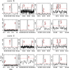 |
Fig. 3 Spectra extracted from the 3σ rms level contour of the 3 mm continuum for cores N (top) and S (bottom) (Fig. 2). The clearly detected transitions are labelled in the eight spectral windows, and the 3σ rms level is represented by the dashed red line. The undetected species, namely HCS+, HCO and HN13C, are not shown. |
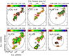 |
Fig. 4 Velocity-integrated molecular emission maps. We show the six molecular species for which the signal-to-noise ratio is good. For C4H, HCS+, HCO, HN13C, and 34SO, the maps are too noisy and we do not show them. The species and the Eup of the line used in temperature units are indicated in the top left corner of each frame. The two stars indicate the peak position of the millimeter-continuum cores N and S. The black circles highlight the primary beam at the rest frequency of each line (Table 2). The integrated emission was computed in the channels in which the intensity was higher than the 3σ rms level. The velocity intervals used are [−18.4;−16.5] km s−1 for c-C3H2; [−19;−16] km s−1 for H13CO+; [−18.75;−16;25] km s−1 for CH3OH (from the line centred at ~96.7414 GHz) at [−20;−14] km s−1 for CS; [−19.5;−15.5] km s−1 for SO; [−18.8;−16.2] km s−1 for H2CO (from the line centred at ~140.8395 GHz). The seven regions highlighted in black are those analysed in detail in Sect. 3.4, and they generally correspond to the 5σ rms emission contour of the corresponding integrated-intensity map (within the ALMA primary beam). |
3.5 Comparison between ALMA and IRAM spectra
The c-C3 H2, H13 CO+, and C4H lines in Table 2 were also observed with the IRAM-30m telescope by Fontani et al. (2022a). To evaluate whether extended emission was resolved out by the interferometer, we extracted the integrated ALMA spectra in flux density units of the mentioned lines from a circular region with a size equal to that of the IRAM 30m telescope main beam (~27″). Then, we converted the IRAM 30m spectra from main-beam temperature units into flux density units through the equation (see e.g. Fontani et al. 2021)
![Mathematical equation: ${F_\nu }[{\rm{mJy}}] = {{{T_{{\rm{MB}}}}[{\rm{K}}]} \over {1222}}v{[{\rm{GHz}}]^2}\Theta {[\prime \prime ]^2},$](/articles/aa/full_html/2024/11/aa51500-24/aa51500-24-eq2.png) (1)
(1)
where Fv is the flux density at the observed rest frequency v, TMB is the main-beam temperature, and Θ is the main-beam angular size of the IRAM 30m telescope at a frequency v.
The comparison is shown in Fig. 5. The flux densities measured with ALMA are consistent with those measured with the IRAM-30m telescope in c-C3H2 and H13CO+ within a factor ≤10%, which is fully consistent with the calibration errors. For C4H, we show in Fig. 5 the J = 19/2−17/2 hyperfine component, for which the difference between the IRAM and ALMA spectra is largest (a factor ~1.3−1.4). Considering the calibration errors and the rms noise in the spectra (in particular in the C4H IRAM 30m spectrum), we conclude that the amount of extended flux that is resolved out by ALMA is negligible and does not affect our analysis significantly.
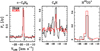 |
Fig. 5 Flux density comparison between ALMA and IRAM 30m spectra. The IRAM 30 m and ALMA spectra are shown as black and red histograms, respectively. The ALMA spectra were extracted from an angular region equivalent to the IRAM 30m beam at the frequency of the lines (~27″). |
4 Spectral analysis and derivation of the column densities
4.1 Spectral analysis
The flux densities were converted into brightness temperatures (TB) according to Eq. (1). This relation needs the observed angular equivalent diameter (i.e. the diameter of the equivalent circle) of each core. Therefore, TB is an average brightness temperature over the solid angle of each core. We analysed the spectra in TB units with the software MAdrid Data CUBe Analysis (MADCUBA3, Martín et al. 2019). The transitions reported in Table 2 were modelled via the toll called Spectral Line Identification and LTE Modelling (SLIM) of MADCUBA. The lines were fitted with the AUTOFIT function of SLIM. This function produces the synthetic spectrum that matches the data best, assuming a constant excitation temperature (Tex) for all transitions of the same species. The other input parameters are the total molecular column density (Ntot), the radial systemic velocity of the source (V), the line FWHM, and angular size of the emission (θs). AUTOFIT assumes that V, FWHM, and θs are the same for all transitions. For θs, we assumed that the emission is more extended than the extraction region in all tracers, and hence, we applied no filling factor to derive the best-fit parameters. Assuming as θs the equivalent radii given in Table 4 would change the resulting column densities by a factor 1.2 at most. We left all other parameters free except for Tex, which we had to fix for all species except for CH3 OH. For this molecule alone, two transitions with significantly different Eu were detected (Table 2). We decided to adopt the Tex measured from CH3OH for all species.
The analysis described above with MADCUBA was adopted for the lines of these species: c-C3H2, CH3OH, H2CO, C4H, and HCS+. For the remaining species, namely HCO, H13CO+, HN13C, CS, SO, and 34SO, MADCUBA was unable to fit the lines in all regions because the observed FWHMs are comparable to the spectral resolution of their spectra (spw 33, 39, and 41 in Band 3). Towards region 5, CH3OH was also not fit for the same reason. Therefore, we obtained the integrated intensities for these species of the lines with the CLASS4 package of the GILDAS software. Ntot were then calculated with the same equations as were used by MADCUBA, namely assuming the LTE at Tex to be equal to that derived from CH3 OH in this case as well. We also assumed optically thin conditions. The assumption is justified both because of the Gaussian line profiles and because the optical depths provided by AUTOFIT for the lines analysed with MADCUBA are consistent with optically thin conditions.
The results we obtained are listed in Table 5. One remarkable immediate result is the low values of the FWHMs of all lines, which are narrower than ~2 km s−1 in both N and S. Even though the cores harbour infrared-bright sources, the FWHMs are narrow and comparable to those measured in starless cores in infrared dark clouds (e.g. Kong et al. 2017; Barnes et al. 2023) rather than to those measured in infrared-bright proto- stellar envelopes (e.g. Fontani et al. 2002, 2023). The excitation temperatures derived from CH3OH are ~9 K and ~15 K in core N and S, respectively. These low temperatures could indicate sub-thermal excitation conditions, at least for CH3OH. Assuming the same Tex for the other molecules, as explained above, we derived Ntot of ~1012 cm−2 for H13CO+and of ~1013 cm−2 for CH3OH, C4H, H2CO, CS, and SO.
As stated above, to derive Ntot we fixed Tex to that of CH3OH for all molecules. This assumption is justified because in all transitions we analysed, the energies of the upper level lie in between ~4 and ~20 K, which is similar to the energy range of the methanol lines (7–20 K). However, the computed low Tex could indicate sub-thermal conditions for CH3OH. We estimated the uncertainty introduced by this simplified approach by varying Tex in between the CH3OH values and a representative kinetic temperature of the gaseous envelope of high-mass protostellar objects of ~30 K (e.g. Sánchez-Monge et al. 2013; Fontani et al. 2015) in the case when the CH3OH emission is sub-thermally excited. The Ntot variation depends on the species and is larger on average for core N, for which the difference between Tex from CH3OH (9 K) and the representative temperature of 30 K is highest. For example, in core N, Ntot of CS increases from 1.7×10¹³ to 2.6×1013 cm−2; Ntot of H13CO+ increases from l.5×1012 to 2.8× 1012 cm−2; c-C3H2 cannot be reasonably fit with a Tex above 15 K when both the detected transition and the upper limit on the transition J(Ka, K, b) = 4(3,2) – 4(2, 3) at ~85.656 GHz are considered, but undetected; Ntot of C4H decreases from 9.1 ×10¹² to 5.5×1012 cm−2; and Ntot of H2CO remains the same within the errors.
Best-fit parameters of the spectra of the millimeter-continuum sources N and S.
4.2 Fractional abundances in the continuum cores
To estimate the molecular fractional abundances with respect to H2, we computed the column density of H2, N(H2), from the integrated continuum flux density through the equation (e.g. Battersby et al. 2014)
 (2)
(2)
where γ is the gas-to-dust mass ratio, Fv is the flux density at frequency v, Ω is the solid angle of the source at the observed frequency, ĸv is the dust opacity, which is usually parametrised as  (Ossenkopf & Henning 1994), Bv(Td) is the Planck function at the dust temperature Td, µ(H2) is the mean molecular weight, for which we adopted 2.8 (Kauffmann et al. 2008), and mH is the mass of the hydrogen atom. Using the empirical relation between γ and RGC derived from Giannetti et al. (2017), we find γ ~ 3000 at RGC = 23.4 kpc. Considering the uncertainties in the Giannetti et al. (2017) empirical relation, γ is
  , hence more than eight times higher than the conventional value of 100. For Td, we adopted the excitation temperature derived from CH3 OH (Table 5) for each core, assuming that gas and dust are coupled. We also assumed a dust opacity index β = 1.7, which is a typical value used for ice-coated dust grains in dense cores, and
  at v0 = 230 GHz (Ossenkopf & Henning 1994). The resulting N(H2) are ~5.7 × 10²¹ and ~2.1 × 1021 cm−2, respectively. Assuming spherical sources, we also computed the core H2 gas masses, Md, and volume densities, n(H2). Md and n(H2) are ~1 M⊙ and ~104 cm−3 , respectively, for both cores. Core N is denser and more massive. All parameters are listed in Table 3. We show the molecular fractional abundances derived from the Ntot-to-N(H2) ratio in Table 5.
These estimates are affected by several uncertainties. First, as discussed in Sect. 4.1, Ntot can vary up to a factor of 2 depending on the species. Second, computing β from the integrated continuum flux densities in the 3 mm and 2 mm bands (Table 3) through Eq. (2) in Chacón-Tanarro et al. (2019b), we find β ~ 0.34 and β ~ 0.21 for core N and S, respectively. With these β, we find N(H2) ~ 1.6 × 1021 cm−2 for N and N(H2) ~ 1.6 × 1021 cm−2 for S, respectively, that is, a factor of ~3 smaller than those given in Table 3. The molecular abundances in Table 5 would therefore systematically increase by the same factor. Another large uncertainty is introduced by the value of  calculated from Giannetti et al. (2017), which causes the abundances to vary up to an additional factor of ~4. The uncertainties on β depend on the measured continuum flux densities and dust temperatures. While the relative error on the continuum flux densities is ~10%, the error on the dust temperature is difficult to quantify. However, we stress that all these uncertainties affect the individual abundances, but not their ratios.
In the diffuse ISM, β is ~2 (e.g. Draine & Lee 1984), while lower values are measured in dense cores (e.g. Forbrich et al. 2015; Galametz et al. 2019) and circumstellar discs (e.g. Testi et al. 2014; Friesen et al. 2018). β can strongly depend on the grain size, composition, and porosity, but values lower than 0.5 are hard to explain without considering large grains with sizes of ~100 µm − 1 mm (e.g. Testi et al. 2014; Ysard et al. 2019). In protoplanetary discs, large grains like this are expected as a result of coagulation and growth. However, cores N and S have a linear diameter ≥30 000 au, and the observed emission is therefore probably not dominated by a circumstellar disc. Values of β lower than one were also measured up to ~2000 au scales around young protostars (e.g. Galametz et al. 2019). This is indicative of early grain growth, although theory is struggling to determine possible reasons for this growth at the relatively low density of the 1000–10 000 au scale of protostellar envelopes. It has been proposed that large grains are not formed on these extended envelope scales, but are transported there from the site of growth via jets and winds (e.g. Cacciapuoti et al. 2024). This scenario might be possible for WB670, but the narrow FWHMs of the observed lines in N and S (Table 5) suggest a very quiescent environment and should therefore be disregarded. Silsbee et al. (2022) proposed that the presence of very small grains could also cause a low β. This scenario may be possible if the distribution of the grain size at the galactocentric distance of WB670 is different from that in the local medium. Other options are also possible, such as high dust opacities and contamination from free-free emission at 3 mm. We did not find any free- free emission study towards WB670 (e.g. from radio-continuum emission), and hence, this option cannot be checked.
4.3 Column densities in the molecule-emitting regions
In Appendix C (available on Zenodo), we list the parameters we obtained by fitting the lines with MADCUBA and CLASS towards the lines detected in the seven regions indicated in Fig. 4. For the continuum cores, the FWHMs are always narrower than 1.5– 2 km s−1, indicating quiescent gas. The Tex derived from the two detected CH3OH lines are in between 6.4 K and 15 K, similar to that measured towards cores N and S. This suggests that the emission arises from cold gas in these regions as well. This is again consistent with the relatively low FWHMs of the lines, which are lower than ~1–2 km s−1 , which furthermore indicates that the emission arises from quiescent material. Regarding Ntot, for CH3OH we derive values of about 1012 – 1013cm−2, with the maximum value (~1.6 × 1013cm−2) in the north-west filament in between core N and the edge of the primary beam. The hydrocarbons C4H and c-C3H2 have similar column densities. Both are ~1012cm−2. For these regions, we cannot derive abundances because we cannot estimate the H2 column densities. We therefore discuss the comparison between the Ntot of the various species in Sect. 5.1.
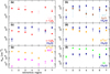 |
Fig. 6 Column density comparison in the seven molecular extraction regions. The colours in the different panels indicate the different molecular species according to the labels in the bottom right corner (top right corner in panel (e)). Empty symbols with a downward-pointing arrow are upper limits. |
5 Discussion
5.1 Comparisons of the column density
In Fig. 6, we compare the molecular column densities between different species in the seven regions of WB670. The relative Ntot of the hydrocarbons C4H and c-C3H2 are similar and do not change significantly in the sub-regions of WB670, as shown in panel (a) of Fig. 6. To form, both species require atomic С that is not locked in CO. Their good agreement in the different regions is therefore consistent with expectations. In panel (b) of Fig. 6, we compare Ntot of H2CO, HCO, and CH3OH, which are thought to be chemically related because all can be formed from hydrogenation of CO on dust grains. Ntot of CH3OH is largely variable in the seven sub-regions, and the trend does not follow that of HCO and H2CO, since the higher Ntot of CH3OH are found where those of HCO and H2CO are lower, and vice versa.
The same dichotomy is also apparent between CH3OH and c-C3H2 (panel c). This is especially evident in region 1, where Ntot of CH3OH is lowest and that of c-C3H2 is highest, and in region 4, where the opposite occurs. A similar dichotomy is observed in the prestellar core L1544 (Spezzano et al. 2016; Jensen et al. 2023), where the emission of the two molecules seems to be anti-correlated. In particular, CH3OH emission arises from colder and more shielded regions of the L1544 core envelope, while c-C3H2 emission overlaps the dust-continuum emission. This observational difference is consistent with the different physical conditions needed to form the two molecules. While it is well known that CH3OH is formed from sequential hydrogenation of CO on grain surfaces (e.g. Fuchs et al. 2009), the formation of c-C3H2 occurs in the gas phase through an ion-molecule reaction that is followed by dissociative recombination (e.g. Sipilä et al. 2016). These reactions do not need a low-temperature and high-density environment as is required for CH3OH formation. Therefore, the dichotomy between these two species likely arises from these different formation routes. Interestingly, the variation of Ntot in the seven regions found for H2CO and HCO (panel b in Fig. 6) resembles that of c-C3H2 more than that of CH3OH. This points to formation routes of H2CO and HCO in the gas phase rather than through surface chemistry processes. In particular, while CH3OH can only be formed on the surfaces of dust grains given the inefficiency of gas-phase routes at low temperatures (e.g. Garrod et al. 2006), H2CO is also known to form in the gas phase from regions that are rich in hydrocarbons, where С is not yet completely locked in CO (see e.g. Chacón-Tanarro et al. 2019a). HCO can also form via gas-phase reactions (Rivilla et al. 2019). Our observations seem to indicate that the gas-phase formation of H2CO and HCO from atomic С is likely more efficient than its formation on dust grains, even though the abundance of С at these large galactocentric distances is higher.
The trends of the molecular ions H13CO+ and HCS+ are also more in line with hydrocarbons and H2CO than with H3OH (panels d and e). This can again be attributed to the exclusive formation of these ions in the gas phase. The species for which the trend in Ntot is most similar to that CH3OH is SO, as indicated in panel f of Fig. 6. This similarity could be explained by their common origin from surface chemistry. In fact, SO is thought to be formed in the gas phase from atomic S (e.g. Vidal et al. 2017), which is more abundant upon grain sputtering than in the diffuse gas.
5.2 Comparison with local and inner Galaxy star-forming regions
When we extrapolate the elemental abundance trends measured by Méndez-Delgado et al. (2022) at the galactocentric distance of WB67O, the oxygen, carbon, and nitrogen fractional abundances should be [O/H]~6.7 ± 2.3 × 10⁻⁵, [C/H]~1.8 ± 0.5 × 10⁻⁵, and [N/H]~5.3 ± 1.3 × 10⁻⁶. The reference values at the solar circle are [O/H]~3.1 ± 1.0 × 10⁻⁴, [C/H]~2.6 ± 0.8 × 10⁻⁴, and [N/H]~4.7 ± 1.4 × 10⁻⁵ (Méndez-Delgado et al. 2022). Therefore, the relative elemental ratios [O/C] and [O/N] should increase from [O/C] ~ 1.2 ± 0.7 and [O/N]~6.6 ± 4.0 to [O/C]~3.7 ± 2.0 and [O/N]~12.6 ± 7.6. The molecular ratio that might be particularly sensitive to changes in the [O/C] ratio in principle is CH3OH/c-C3H2 as was found in the prestellar core L1544 (e.g. Spezzano et al. 2016), because for CH3OH to form, carbon needs to be locked in CO, and for c-C3H2 to form, free atomic carbon is required. Figure 7 shows the column density ratios CH3OH/c-C3H2 in the seven molecular regions of WB67O. We compare them to the ratios measured in local (low- and high-mass) star-forming regions (Higuchi et al. 2018) and in the outer Galaxy hot core WB89-789 (hereafter WB789, Shimonishi et al. 2021). As representatives of local low-mass star-forming regions, we took the cores in the Perseus molecular clouds observed by Higuchi et al. (2018). As representatives of high-mass star-forming regions, we took IRAS 20126 and AFGL 2591 (Freeman et al. 2023). The resolved linear scale is ~5000–10 000 au in Higuchi et al. (2018), while it is ~200 000 au in (Freeman et al. 2023). The CH3OH/c-C3H2 ratios derived in WB670 agree on average with the lower values measured in local star-forming regions, while the ratio found in WB789 is twice the highest local values (Fig. 7). Because WB789 is located in between the local Galaxy and WB67O, no monothonic trend of the CH3OH/c-C3H2 ratio with galactocentric distance is apparent. We discuss the comparison between WB670 and WB789 in Sect. 5.3 in more detail.
We also verified whether the column density ratios we derived in WB670 between species that differ by just one element, such as HN13C and H13CO+ and CS and SO, might be attributed to the change in elemental ratios with RGC. Figure 8 shows the column density ratios SO/CS (panel (a)). Despite a dispersion of one order of magnitude, the average value is SO/CS~1.2. Fontani et al. (2023) found average SO/13CS ratios ~ 11–12 in a sample of high-mass star-forming cores in different evolutionary stages, and in the local and inner Galaxy. This ratio translates into ~0.2 when we consider a conversion factor 12C/13C~68 for the local ISM (Milam et al. 2005) (dashed line in panel (a) of Fig. 8). When we scale this value for the increase in the [O/C] elemental ratio (~3.1) from the solar circle to RGC ~ 23.4 kpc (Méndez-Delgado et al. 2022), the expected [SO/CS] column density ratio in WB670 should be ~0.62, that is, a factor of 2 lower than the average measured ratio. The dispersion is such, however, that the measured ratios are consistent overall with those measured in the solar neighbourhoods scaled for metallicity. Panel (b) of Fig. 8 shows the H13CO+/HN13C column density ratios measured in WB67O. The average value is ~2.6. In this case, the dispersion is only a factor of ~2. In local and inner Galaxy star-forming regions, this molecular ratio is very variable. Vasyunina et al. (2011) measured an average HCOVHNC ratio of ~10 in infrared-dark clouds. Zinchenko et al. (2009) found H13CO+/HN13C~1 in a sample of high-mass star-forming regions, indicating that this ratio can be very sensitive to changes in the physical conditions. Because WB670 contains infrared-bright objects, its physical conditions are likely similar to those of the active star-forming regions observed by Zinchenko et al. (2009). This means that the observed H13CO+/HN13C column density ratio increases by a factor of 2.6 on average from local star-forming regions to RGC ~ 23.4 kpc, while the expected increase in the [O/N] elemental ratio should be ~1.8. Therefore, the increased elemental abundance ratio again fails to fully explain the observed molecular ratios. However, considering the dispersion of the values in the literature and the error introduced by the assumed Tex in our analysis, the ratios are consistent overall with a metallicity-scaled trend. On the other hand, the elemental ratios beyond RGC ~ 15 kpc are poorly constrained by observations (e.g. Romano et al. 2020) and have uncertainties up to ~30% on the individual elemental abundances (Méndez-Delgado et al. 2022). Extrapolating them to this large an RGC might therefore be inaccurate.
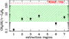 |
Fig. 7 Column density ratio CH3OH/c-C3H2 in WB670 and other star-forming regions. The black points indicate the ratios measured in the seven regions of WB670 (with the exception of region 5, for which both column density estimates are upper limits). The green area corresponds to the range of values measured in local star-forming regions (Higuchi et al. 2018), and the dashed red line is the ratio measured in the outer Galaxy hot core WB789 (Shimonishi et al. 2021). |
5.3 Comparison with sub-solar metallicity hot cores
Some species detected in WB67O were also detected in the hot core WB789 (Shimonishi et al. 2021), located at RGC ~ 19 kpc. The species in common are c-C3H2, CH3OH, H2CO, H13CO+ SO, and CS. Shimonishi et al. (2021) derived two abundance values that were computed on linear diameters of 0.026 and 0.1 pc, respectively. For the comparison with N and S, we used the 0.1 pc values because this size is more similar to that of N and S (Table 3). Figure 9 shows the comparison: Except for SO, all other species show abundances that differ significantly from each other, indicating a clear different chemical composition. In particular, the CH3OH abundance in WB789 is higher by two orders of magnitude than in N and S, while the abundances of all other carbon-bearing species are lower. The CH3OH abundance in WB789 is 2 × 10⁻⁷, while in N and S, it is 0.4 × 10⁻⁹ and 11 × 10−9, respectively. Even considering the abundances obtained assuming β in Table 3, which are higher by a factor of ~3 than those listed in Table 5, the CH3OH abundances in N, S, and WB789 are not consistent. Shimonishi et al. (2021) proposed a chemical stratification of the environment of the WB789 hot core, with CH3OH and all COMs arising from the inner (≤ 0.015 pc) warm (≥ 100 K) region, and SO, CS, H2CO, c-C3H2, H13CO+ and HN13C all associated with an external (≥ 0.05 pc) cold (≤ 40 K) envelope. Our findings also indicate that the species we detect are associated with relatively cold and quiescent envelope material, including CH3OH. However, the line widths in WB789 always exceed ~2 km s−1 even in the envelope tracers, indicating that WB670 and WB789 are different types of star-forming regions. Simulations show that the abundance of CH3OH in a dense star-forming core is extremely sensitive to dust-temperature variations (Acharyya & Herbst 2015; Pauly & Garrod 2018). In particular, the CH3OH production on grain surfaces depends on the duration of the early cold phase in which CO is hydrogenated on grain mantles because atomic hydrogen is highly volatile (see also Shimonishi et al. 2020).
The CH3OH abundances in N and S are comparable to the so-called organic-poor hot cores detected in the Large Magellanic Cloud (LMC, Shimonishi et al. 2020; Hamedani Golshan et al. 2024), which are characterised by values that cannot simply be explained scaling the abundances measured in the local Galaxy for the decreased metallicity (about a factor 2–3, e.g. Andrievsky et al. 2001; Rolleston et al. 2002) of the LMC. Shimonishi et al. (2020) proposed that these organic-poor hot cores in the LMC might be caused by dust temperatures that are higher than those in organic-rich hot cores. Therefore, the lower CH3OH abundance in WB670 could be caused by an inefficient (or insufficient) hydrogenation of CO in the stage of ice formation, by either a (too) warm dust temperature, by to a (too) short cold-ice formation stage, or by a (too) low gas density. All scenarios would also predict a lower production efficiency of H2CO on ice mantles, and this would agree with our finding that H2CO is probably formed in the gas phase in WB670. Alternatively, WB670 can be in a late(r) evolutionary stage than WB789, at which the molecules in the inner protostel-lar cocoon(s), including those that evaporated from dust grain mantles, have been mostly dissociated by the strong protostel-lar radiation field. Pauly & Garrod (2018) proposed that CH3OH abundance might even be enhanced in low-metallicity environments, owing to the lower C/O ratio, which would imply that most of С is locked in CO, which is needed to form CH3OH. However, this scenario would predict that the CH3OH abundance in WB670 is higher than in WB789 because the C/O ratio in WB670 is lower than in WB789 (according to the elemental trends with RGC; see Sect. 1). This is clearly at odds with our observational results. We discuss the influence of the metallicity on the observed molecular abundances in Sect. 5.4 in more detail.
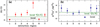 |
Fig. 8 Column density ratios in the seven molecular extraction regions of WB67O. Panel (a) shows the measured SO/CS ratios (points) and compares them to the average SO/CS ratio measured in a sample of inner and local Galaxy high-mass star-forming regions (Fontani et al. 2023, dashed line) and to the expected SO/CS ratio obtained by multiplying the local measured value (0.2, dashed line) by the increase in the elemental ratio [O/C]~3.1 (horizontal green line) from the solar circle to RGC = 23.4 kpc (Méndez-Delgado et al. 2022). Panel (b) shows the same comparison between the measured H13CO+/HN13C ratio and the expected ratio obtained by multiplying the local measured value for the increase in the [O/N] elemental ratio. |
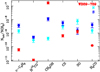 |
Fig. 9 Fractional abundances with respect to H2 derived for N, S, and WB789. The WB789 abundances were derived on a hot-core linear size of 0.1 pc (Shimonishi et al. 2021). |
5.4 Chemical modelling
To better investigate whether the measured column density ratios can constrain the initial elemental abundances as well as other physical parameters that cannot be derived from the data, we compared our observational results to the prediction of chemical models. We investigated these clouds with the open-source gas-grain chemistry code UCLCHEM (Holdship et al. 2017). This time-dependent astrochemical code allowed us to model the evolution of each molecule. We considered a static model, namely an isothermal cloud at constant density with a radius of R = 0.5 pc (the maximum radius of the modelled regions), and we explored a range of physical and chemical conditions. The parameters included the H2 number density (cm−3), the gas temperature, the cosmic-ray ionisation rate ζ, the radiation field FUV, and both the initial oxygen and carbon abundances as listed in Table 6. Each of the models was ran with an edge visual extinction of Av = 1.0 mag, and the molecular ratios were computed at 106 years. The grid is discussed in more detail in Vermariën et al. (in prep.). We converted between 12C and 13C using a conversion factor of 1018 (~68) since the chemical network did not include isotopologues. For the modelling, we used a conventional gas-to-dust mass ratio of 100. We discuss the details of using the observed value obtained from Giannetti et al. (2017) at the end of this section.
We excluded models for which the predicted fractional abundances of our molecules was below 10−13. This resulted in a total of 710 models out of the original 65536. These models were then compared to the observations, and we show the distributions of the fit of the theoretical ratios with the observed ones in Fig. 10, sorted in descending averaged mean squared error between the models and observations. Some ratios, namely CS/HCO+, CS/SO, HCO+/H2CO, HCO+/HCS+, SO/H2CO, SO/HCS+, CS/HCO, HCO/H2CO and CS/HNC, do no overlap between the models and the observations. Some observed ratios also lie in the tails of the model distribution. It is very unlikely overall to find a model that fits all ratios well.
In order to further constrain the physical parameter space, the 50 models with the lowest mean square error (MSE) were chosen. Figure 11 again shows the comparison between the models and the observations. The distribution of the models is now closer to the observations, so that the horizontal axis is more compact than in Fig. 10. Many of the ratio distances between the models and observations decrease considerably when we take only the best models, but the CS-, HCS+-, and H2CO-based ratios do not improve.
In addition to the ratios that could not be explained by just the observable ratios, some ratios also have no matching distribution with the subset of the best models. It does show, however, that we can fit many of the ratios well with the subset of the best models. By plotting the error for each of the ratios in a pairwise grid, as shown in Fig. 12, we can better understand which molecules have the lowest error. This shows the molecules that fit best in the following order: c-C3H2, HNC, HCO, C4H, CH3OH, HCO+, SO, H2CO, HCS+, and finally, CS. We then plot the distribution of the physical and chemical parameters we investigated in the grid (Fig. 13). The models indicate densities ranging from 103 to 103 6 cm−3, temperatures from 20 to 45 K, radiation fields lower than 5 Habing, and a cosmic-ray ionisation rate ζ in a wide range from the interstellar value of ~ 10−17 s−1 up to ~10−14 s−1. Initial abundances of oxygen and carbon higher than one-fifth of the solar value are favoured by the models. Additionally, the [O/C] ratio favours values in between ~2 and 5, with a small distribution of even higher oxygen enhancements. The densities measured in N and S are higher (~104 cm−3) than the values predicted by the models, which refer to the molecular regions, however, and are all more extended than N and S. Moreover, assuming β as in Table 3 to compute N(H2), we derive densities of ~103 cm−3, which is consistent with the model predictions.
Lastly, we investigated the time dependence of these ratios (Fig. 14, available on Zenodo) in order to gauge whether the observed star-forming regions exhibit a younger or older chemical history. Figure 14 shows that for most molecules, the fits would not improve at another time, except for the H2O/CH3OH, CS/HNC, and CS/SO ratios, which might benefit from sampling at a later time. However, this would worsen the fits for other ratios. For some molecules, there seems to be no time at which the ratios are fit correctly. The worst-performing molecule, CS, clearly shows an over-prediction in the model as compared to the observations. However, this inconsistency might be caused by a neglected high optical depth in the derivation of the observed column densities.
Overall, our results indicate that static models such as those investigated here can give a range of physical parameters that match the observations best, but are not optimal for reproducing the set of observed abundances. A more proper fit for each region would need a dynamical modelling that accounts for collapse during the time-dependent evolution. The range of values predicted from the static models suggests that low-energy conditions, in particular, low temperatures (20–45 K) and FUV lower than 5 Habing, are favoured. This is consistent with the location of the source in the Galactic anti-centre (certainly more quiescent than the local and inner Galaxy). The models also predict that the oxygen elemental abundance should not be lower than one-fifth of the solar value, which is consistent with an extrapolation of the Méndez-Delgado et al. (2022) trend, which predicts a decrease of a factor 4.6. The carbon elemental abundance should also not be lower than ~ one-fifth of the solar value, but this is well above the value extrapolated from the Méndez-Delgado et al. (2022) trend at 23.4 kpc, which is ~1/14th of the solar value. If confirmed by models that include dynamical collapse, this difference would indicate a [C/H] gradient that flattens in the far outer Galaxy with respect to the trend derived at inner RGC. Elemental galactocentric gradients derived from observations of HII regions in spiral galaxies characterised by extended H I envelopes indeed indicate a flattening of the radial distribution of metals at large galactocentric distances (Bresolin 2017). An elemental gradient of carbon flatter than expected in the OG would also explain why the abundance trends with RGC of organ-ics tend to be fainter than the extrapolated gradients (Bernal et al. 2021; Fontani et al. 2022b).
Another caveat arises from the assumed gas-to-dust mass ratio, which could be higher than we assumed (100) according to the trend proposed by Giannetti et al. (2017)  . We thus performed two tests, one for a model at low density (~103 cm−3), and one at high density (~106 cm−3). In the low-density case, the results show no significant differences. In the high-density case, some differences are found, but this case does not represent WB670. Moreover, no firm measurements of this ratio were obtained so far at an RGC this large, to our knowledge. Aassuming a gas-to-dust ratio that is significantly different from the standard one therefore introduces further uncertainty in the models.
Ranges of physical and chemical parameters of the grid of models.
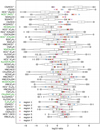 |
Fig. 10 Comparison of the distribution of log-ratios of the observed species. The ratios shown in Fig. 6 are highlighted in green. The seven observed region ratios (coloured markers) are plotted against the distribution of the modelled ratios (grey box plots). The molecules are sorted from top to bottom in order of decreasing error. |
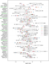 |
Fig. 11 Fifty best models (grey box plots) compared to the seven observed regions (coloured markers). |
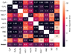 |
Fig. 12 Mean squared error computed between all of the regions and the 50 best models. The averaged MSE for each molecule is included in the bottom row. |
6 Conclusions
We used ALMA to observe WB670, the source at the largest galactocentric distance (23.4 kpc) in CHEMOUT, at a resolution of ~15000 au. We detected emission of c-C3H2, C4H, CH2OH, H2CO, HCO, H13CO+, HCS+, CS, HN13C, and SO, derived their column densities, and compared the observational results with chemical model predictions. The main results of our study are listed below.
The molecular emission arises from a filamentary structure oriented SE-NW, where multiple cores are detected. The filament seems more extended than the ALMA primary beam. The morphology is different in each tracer. The most intense emission of molecular ions, carbon-chain molecules, and H2CO is associated with the millimeter-continuum infrared-bright cores. In contrast, the most intense CH3OH and SO emission predominantly arises from the part of the filament that lacks continuum sources. The narrow line widths (~1– 2 km s−1) across the filament indicate quiescent gas, despite the presence of the infrared-bright sources.
From an LTE analysis of the CH3OH lines, their excitation temperatures are quite low (7–15 K) and could be under-thermally excited. The derived molecular column densities are comparable with those in local star-forming regions. There seems to be a spatial anti-correlation between the column density of hydrocarbons, molecular ions, HCO, and H2CO on one hand, and CH3OH and SO on the other. This might suggest different formation processes for the two groups of molecules (gas-phase processes versus surface processes).
CH3OH fractional abundances calculated towards the millimeter-continuum cores (0.4−11 × 10−9) are consistent with those of the so-called organic-poor cores found in the LMC, where these low CH3OH abundances might be due to an inefficient hydrogenation of CO on grain mantles.
Static models that match the observed column densities best favour diffuse gas and low-irradiation conditions (expected at large galactocentric radii), but carbon element abundances that are three times higher than the abundance derived by extrapolating the [C/H] elemental galactocentric gradient at 23 kpc. This would indicate a flatter [C/H] trend at large galactocentric radii, which is in line with a flat abundance of the organics. Models including dynamical evolution should be able to reproduce the chemical composition of WB670 better.
The results of this work indicate that a proper comparison between observations and models starting from a huge grid of parameters is essential to model the chemistry properly. Our study would greatly benefit from new observations of more molecular species and more lines at the same (at least) spatial resolution as we obtained here. In particular, tracers of the cosmic-ray ionisation rate, which is basically unconstrained by our study, are relevant.
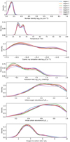 |
Fig. 13 Kernel density probability estimate of the physical parameters for the 50 best models, fit separately for each of the regions, indicated by the coloured curves as labelled in the top right corner. |
Data availability
Figure 14 and Appendices A–C can be found at https://zenodo.org/records/13884598?preview=1&token=eyJhbGciOiJIUzUxMiJ9.eyJpZCI6IjhjNWU4MTY5LWFlMjctNDZiOS1hNjc1LTJmMjYxNjQ4MzdjZiIsImRhdGEiOnt9LCJyYW5kb20iOiIxZDUwODczOTVhMjg0YTdhMWUxZjc1ODI1MWFkOTE2YyJ9.2IrOMtrRtswzvxGsoIRZhcWXW2Vi00Ij5II0YklKTp6SmwfTAxJML5T2gmNtfZZ8dJtJREJEPYzGJvhxmSmsg
Acknowledgements
This paper makes use of the following ALMA data: ADS/JAO.ALMA#2022.1.00911.S. ALMA is a partnership of ESO (representing its member states), NSF (USA) and NINS (Japan), together with NRC (Canada), MOST and ASIAA (Taiwan), and KASI (Republic of Korea), in cooperation with the Republic of Chile. The Joint ALMA Observatory is operated by ESO, AUI/NRAO and NAOJ. F.F., S.V., G.V., and D.G. acknowledge support from the European Research Council (ERC) Advanced grant MOPPEX 833460. L.C. and V.M.R. acknowledges support from the grant PID2022-136814NB-100 by the Spanish Ministry of Science, Innovation and Universities/State Agency of Research MICIU/AEI/10.13039/501100011033 and by ERDF, UE; V.M.R. also acknowledge support from the grant RYC2020-029387-I funded by MICIU/AEI/10.13039/501100011033 and by “ESF, Investing in your future”, and from the Consejo Superior de Investigaciones Científicas (CSIC) and the Centro de Astrobiología (CAB) through the project 20225AT015 (Proyectos intramurales especiales del CSIC); and from the grant CNS2023-144464 funded by MICIU/AEI/10.13039/501100011033 and by “European Union NextGener-ationEU/PRTR”. A.S.-M. acknowledges support from the RyC2021-032892-I grant funded by MCIN/AEI/10.13039/501100011033 and by the European Union ‘Next GenerationEU’/PRTR, as well as the program Unidad de Excelencia María de Maeztu CEX2020-001058-M, and support from the PID2020-117710GB-I00 (MCI-AEI-FEDER, UE).
References
- Acharyya, K., & Herbst, E. 2015, ApJ, 812, 142 [NASA ADS] [CrossRef] [Google Scholar]
- Andrievsky, S. M., Kovtyukh, V. V., Korotin, S. A., et al. 2001, A&A, 367, 605 [NASA ADS] [CrossRef] [EDP Sciences] [Google Scholar]
- Arellano-Córdova, K. Z., Esteban, C., García-Rojas, J., Méndez-Delgado, J. E. 2020, MNRAS, 496, 1051 [CrossRef] [Google Scholar]
- Barnes, A. T., Lui, J., Zhang, Q., et al. 2023, A&A, 675, A53 [NASA ADS] [CrossRef] [EDP Sciences] [Google Scholar]
- Battersby, C., Ginsburg, A., Bally, J., et al. 2014, ApJ, 787, 113 [NASA ADS] [CrossRef] [Google Scholar]
- Bernal, J. J., Sephus, C. D., & Ziurys, L. M. 2021, ApJ, 922, 106 [NASA ADS] [CrossRef] [Google Scholar]
- Blair, S. K., Magnani, L., Brand, J., & Wouterloot, J. G. A. 2008, AsBio, 8, 59 [NASA ADS] [Google Scholar]
- Bresolin, F. 2017, ASSL, 434, 145 [Google Scholar]
- Buchhave, L. A., Latham, D. W., Johansen, A., et al. 2012, Nature, 486, 375 [NASA ADS] [Google Scholar]
- Cacciapuoti, L., Testi, L., Podio, L., et al. 2024, ApJ, 961, 90 [NASA ADS] [CrossRef] [Google Scholar]
- Chacón-Tanarro, A., Caselli, P., Bizzocchi, L., et al. 2019a, A&A, 622, 141 [Google Scholar]
- Chacón-Tanarro, A., Pineda, J. E., Caselli, P., et al. 2019b, A&A, 623, A118 [NASA ADS] [CrossRef] [EDP Sciences] [Google Scholar]
- Colzi, L., Romano, D., Fontani, F., et al. 2022, A&A, 667, A151 [NASA ADS] [CrossRef] [EDP Sciences] [Google Scholar]
- Cutri, R. M., et al. 2003, The IRSA 2MASS All-Sky Point Source Catalogue, NASA/IPAC Infrared Science Archive. Available at: http://irsa.ipac.caltech.edu/applications/Gator/ [Google Scholar]
- Draine, B. T., & Lee, H. M. 1984, ApJ, 285, 89 [NASA ADS] [CrossRef] [Google Scholar]
- Endres, P., Schlemmer, S., Schilke, P., Stutzki, J., & Müller, H.S.P. 2016, J. Mol. Spectrosc., 327, 95 [NASA ADS] [CrossRef] [Google Scholar]
- Esteban, C., Fang, X., García-Rojas, J., & Toribio San Cipriano, L. 2017, MNRAS, 471, 987 [NASA ADS] [CrossRef] [Google Scholar]
- Fontani, F., Cesaroni, R., Caselli, P., & Olmi, L. 2002, A&A, 389, 603 [NASA ADS] [CrossRef] [EDP Sciences] [Google Scholar]
- Fontani, F., Busquet, G., Palau, Aina, et al. 2015, A&A, 575, A87 [NASA ADS] [CrossRef] [EDP Sciences] [Google Scholar]
- Fontani, F., Barnes, A.T., Caselli, P., et al. 2021, MNRAS, 503, 4320 [NASA ADS] [CrossRef] [Google Scholar]
- Fontani, F., Colzi, L., Bizzocchi, L., et al. 2022a, A&A, 660, A76 [NASA ADS] [CrossRef] [EDP Sciences] [Google Scholar]
- Fontani, F., Schmiedeke, A., Sánchez-Monge, Á., et al. 2022b, A&A, 664, A154 [NASA ADS] [CrossRef] [EDP Sciences] [Google Scholar]
- Fontani, F., Roueff, E., Colzi, L., & Caselli, P. 2023, A&A, 680, A58 [NASA ADS] [CrossRef] [EDP Sciences] [Google Scholar]
- Forbrich, J., Lada, C.J., Lombardi, M., et al. 2015, A&A, 580, A114 [NASA ADS] [CrossRef] [EDP Sciences] [Google Scholar]
- Freeman, P., Bottinelli, S., Plume, R., et al. 2023, A&A, 678, A18 [NASA ADS] [CrossRef] [EDP Sciences] [Google Scholar]
- Friesen, R. K., Pon, A., Bourke, T. L., et al. 2018, ApJ, 869, 158 [NASA ADS] [CrossRef] [Google Scholar]
- Fuchs, G. W., Cuppen, H. M., Ioppolo, S., et al. 2009, A&A, 505, 629 [NASA ADS] [CrossRef] [EDP Sciences] [Google Scholar]
- Galametz, M., Maury, A. J., Valdivia, V., et al. 2019, A&A, 632, A5 [NASA ADS] [CrossRef] [EDP Sciences] [Google Scholar]
- Garrod, R., Park, I. H., Caselli, P., & Herbst, E. 2006, FaDi, 133, 51 [NASA ADS] [Google Scholar]
- Giannetti, A., Leurini, S., König, S., et al. 2017, A&A, 606, L12 [NASA ADS] [CrossRef] [EDP Sciences] [Google Scholar]
- Gonzalez, G., Brownlee, D., & Ward, P. 2001, Icarus, 152, 185 [Google Scholar]
- Hamedani Golshan, R., Sánchez-Monge, Á., Schilke, P., et al. 2024, A&A, 688, A3 [NASA ADS] [CrossRef] [EDP Sciences] [Google Scholar]
- Higuchi, A. E., Sakai, N., Watanabe, Y., et al. 2018, ApJS, 236, 52 [Google Scholar]
- Holdship, J., Viti, S., Jiménez-Serra, I., et al. 2017, AJ, 154, 38 [NASA ADS] [CrossRef] [Google Scholar]
- Jensen, S. S., Spezzano, S., Caselli, P., Grassi, T., & Haugbølle, T. 2023, A&A, 675, A34 [NASA ADS] [CrossRef] [EDP Sciences] [Google Scholar]
- Kauffmann, J., Bertoldi, F., Bourke, T. L., et al. 2008, A&A, 487, 993 [NASA ADS] [CrossRef] [EDP Sciences] [Google Scholar]
- Kong, S., Tan, J. C., Caselli, P., et al. 2017, ApJ, 834, 193 [NASA ADS] [CrossRef] [Google Scholar]
- López-Corredoira, M., Allende Prieto, C., Garzón, F., et al. 2018, A&A, 612 L8 [EDP Sciences] [Google Scholar]
- Maliuk, A., & Budaj, J. 2020, A&A, 635, A191 [NASA ADS] [CrossRef] [EDP Sciences] [Google Scholar]
- Martín, S., Martín-Pintado, J., Blanco-Sánchez, C., et al. 2019, A&A, 631, A159 [Google Scholar]
- Méndez-Delgado, J. E., Amayo, A., Arellano-Córdova, K. Z., et al. 2022, MNRAS, 510, 4436 [CrossRef] [Google Scholar]
- Milam, S. N., Savage, C., Brewster, M. A., & Ziurys, L. M. 2005, ApJ, 634, 1126 [NASA ADS] [CrossRef] [Google Scholar]
- Ossenkopf, V., & Henning, Th. 1994, A&A, 291, 943 [NASA ADS] [Google Scholar]
- Pauly, T., & Garrod, R.T. 2018, ApJ, 854, 13 [NASA ADS] [CrossRef] [Google Scholar]
- Pickett, H. M., Poynter, R. L., Cohen, E. A., et al. 1998, JQSRT, 60, 883 [NASA ADS] [CrossRef] [Google Scholar]
- Ramírez, I., Asplund, M., Baumann, P., Meléndez, J., & Bensby, T. 2010, A&A, 521, A33 [Google Scholar]
- Ramal-Olmedo, J. C., Menor-Salván, C. A., & Fortenberry, R. C. 2021, A&A, 656, A148 [NASA ADS] [CrossRef] [EDP Sciences] [Google Scholar]
- Rivilla, V. M., Beltrán, M. T., Vasyunin, A., et al. 2019, MNRAS, 483, 806 [NASA ADS] [CrossRef] [Google Scholar]
- Rolleston, W. R. J., Trundle, C., & Dufton, P. L. 2002, A&A, 396, 53 [NASA ADS] [CrossRef] [EDP Sciences] [Google Scholar]
- Romano, D., Franchini, M., Grisoni, V., et al. 2020, A&A, 639, A37 [NASA ADS] [CrossRef] [EDP Sciences] [Google Scholar]
- Sánchez-Monge, Á., Palau, A., Fontani, F., et al. 2013, MNRAS, 432, 3288 [CrossRef] [Google Scholar]
- Sewilo, M., Indebetouw, R., Charnley, S. B., et al. 2018, ApJ, 853, L19 [CrossRef] [Google Scholar]
- Shimonishi, T., Watanabe, Y., Nishimura, Y., et al. 2018, ApJ, 891, 164 [Google Scholar]
- Shimonishi, T., Das, A., Sakai, N., et al. 2020, ApJ, 891, 164 [NASA ADS] [CrossRef] [Google Scholar]
- Shimonishi, T., Izumi, N., Furuya, K., & Yasui, C. 2021, ApJ, 922, 206 [NASA ADS] [CrossRef] [Google Scholar]
- Silsbee, K., Akimkin, V., Ivlev, A. V., et al. 2022, ApJ, 940, 188 [NASA ADS] [CrossRef] [Google Scholar]
- Sipilä, O., Spezzano, S., & Caselli, P. 2016, A&A, 591, L1 [NASA ADS] [CrossRef] [EDP Sciences] [Google Scholar]
- Spezzano, S., Bizzocchi, L., Caselli, et al. 2016, A&A, 592, L11 [NASA ADS] [CrossRef] [EDP Sciences] [Google Scholar]
- Testi, L., Birnstiel, T., Ricci, L., et al. 2014, Protostars and Planets VI, eds. H. Beuther, R. S. Klessen, C. P. Dullemond, & T. Henning (Tucson: University of Arizona Press), 339 [Google Scholar]
- Vasyunina, T., Linz, H., Henning, Th., et al. 2011, A&A, 527, A88 [NASA ADS] [CrossRef] [EDP Sciences] [Google Scholar]
- Vidal, T. H. G., Loison, J.-C., Jaziri, A. Y., et al. 2017, MNRAS, 469, 435 [Google Scholar]
- Wright, E. L., et al. 2010, AJ, 140, 1868 [NASA ADS] [CrossRef] [Google Scholar]
- Ysard, N., Koehler, M., Jiménez-Serra, I., et al. 2019, A&A, 631, A88 [NASA ADS] [CrossRef] [EDP Sciences] [Google Scholar]
- Wouterloot, J. G. A., & Brand, J. 1989, A&AS, 80, 149 [NASA ADS] [Google Scholar]
- Zinchenko, I., Caselli, P., & Pirogov, L. 2009, MNRAS, 395, 2234 [NASA ADS] [CrossRef] [Google Scholar]
MADCUBA is developed in the Madrid Center of Astrobiology (INTA-CSIC) and enables us to visualise and analyse single spectra and data cubes. https://cab.inta-csic.es/madcuba/
All Tables
All Figures
|
Fig. 1 Near- and mid-infrared images of WB89-670. The panels in the top row show the images at 1.25 µm (H) and 2.15 µm (Ks) from the 2MASS survey. The panels in the bottom row show the WISE images at the wavelengths indicated in the top left corner. The white circles are the ALMA primary beams at ~86 GHz and ~150 GHz, which are 66″ (i.e. ~7.5 pc) and 38″ (i.e. ~4.3 pc), respectively. |
| In the text | |
|
Fig. 2 Continuum emission detected towards WB89-670 with ALMA. The light blue contours in the left and right panels correspond to the 3 mm and 2 mm continuum emission, respectively. Contours start from the 3σ rms level (~8 × 10⁻⁵ Jy at 3 mm and ~3 × 10⁻⁴ Jy at 2 mm), and are in steps of ~5 × 10⁻⁵ Jy and ~2 × 10⁻⁴ Jy, respectively. The synthesised beam is depicted in the bottom left corner, and the white circle indicates the ALMA primary beam at the two wavelengths. The region shown in the 2 mm images corresponds to the dashed square illustrated in the top left panel. The heat-colour image in background is the Ks band of 2MASS (Fig. 1) in the top panels and the WISE 22µm band in the bottom panels. |
| In the text | |
|
Fig. 3 Spectra extracted from the 3σ rms level contour of the 3 mm continuum for cores N (top) and S (bottom) (Fig. 2). The clearly detected transitions are labelled in the eight spectral windows, and the 3σ rms level is represented by the dashed red line. The undetected species, namely HCS+, HCO and HN13C, are not shown. |
| In the text | |
|
Fig. 4 Velocity-integrated molecular emission maps. We show the six molecular species for which the signal-to-noise ratio is good. For C4H, HCS+, HCO, HN13C, and 34SO, the maps are too noisy and we do not show them. The species and the Eup of the line used in temperature units are indicated in the top left corner of each frame. The two stars indicate the peak position of the millimeter-continuum cores N and S. The black circles highlight the primary beam at the rest frequency of each line (Table 2). The integrated emission was computed in the channels in which the intensity was higher than the 3σ rms level. The velocity intervals used are [−18.4;−16.5] km s−1 for c-C3H2; [−19;−16] km s−1 for H13CO+; [−18.75;−16;25] km s−1 for CH3OH (from the line centred at ~96.7414 GHz) at [−20;−14] km s−1 for CS; [−19.5;−15.5] km s−1 for SO; [−18.8;−16.2] km s−1 for H2CO (from the line centred at ~140.8395 GHz). The seven regions highlighted in black are those analysed in detail in Sect. 3.4, and they generally correspond to the 5σ rms emission contour of the corresponding integrated-intensity map (within the ALMA primary beam). |
| In the text | |
|
Fig. 5 Flux density comparison between ALMA and IRAM 30m spectra. The IRAM 30 m and ALMA spectra are shown as black and red histograms, respectively. The ALMA spectra were extracted from an angular region equivalent to the IRAM 30m beam at the frequency of the lines (~27″). |
| In the text | |
|
Fig. 6 Column density comparison in the seven molecular extraction regions. The colours in the different panels indicate the different molecular species according to the labels in the bottom right corner (top right corner in panel (e)). Empty symbols with a downward-pointing arrow are upper limits. |
| In the text | |
|
Fig. 7 Column density ratio CH3OH/c-C3H2 in WB670 and other star-forming regions. The black points indicate the ratios measured in the seven regions of WB670 (with the exception of region 5, for which both column density estimates are upper limits). The green area corresponds to the range of values measured in local star-forming regions (Higuchi et al. 2018), and the dashed red line is the ratio measured in the outer Galaxy hot core WB789 (Shimonishi et al. 2021). |
| In the text | |
|
Fig. 8 Column density ratios in the seven molecular extraction regions of WB67O. Panel (a) shows the measured SO/CS ratios (points) and compares them to the average SO/CS ratio measured in a sample of inner and local Galaxy high-mass star-forming regions (Fontani et al. 2023, dashed line) and to the expected SO/CS ratio obtained by multiplying the local measured value (0.2, dashed line) by the increase in the elemental ratio [O/C]~3.1 (horizontal green line) from the solar circle to RGC = 23.4 kpc (Méndez-Delgado et al. 2022). Panel (b) shows the same comparison between the measured H13CO+/HN13C ratio and the expected ratio obtained by multiplying the local measured value for the increase in the [O/N] elemental ratio. |
| In the text | |
|
Fig. 9 Fractional abundances with respect to H2 derived for N, S, and WB789. The WB789 abundances were derived on a hot-core linear size of 0.1 pc (Shimonishi et al. 2021). |
| In the text | |
|
Fig. 10 Comparison of the distribution of log-ratios of the observed species. The ratios shown in Fig. 6 are highlighted in green. The seven observed region ratios (coloured markers) are plotted against the distribution of the modelled ratios (grey box plots). The molecules are sorted from top to bottom in order of decreasing error. |
| In the text | |
|
Fig. 11 Fifty best models (grey box plots) compared to the seven observed regions (coloured markers). |
| In the text | |
|
Fig. 12 Mean squared error computed between all of the regions and the 50 best models. The averaged MSE for each molecule is included in the bottom row. |
| In the text | |
|
Fig. 13 Kernel density probability estimate of the physical parameters for the 50 best models, fit separately for each of the regions, indicated by the coloured curves as labelled in the top right corner. |
| In the text | |
Current usage metrics show cumulative count of Article Views (full-text article views including HTML views, PDF and ePub downloads, according to the available data) and Abstracts Views on Vision4Press platform.
Data correspond to usage on the plateform after 2015. The current usage metrics is available 48-96 hours after online publication and is updated daily on week days.
Initial download of the metrics may take a while.