| Issue |
A&A
Volume 687, July 2024
|
|
|---|---|---|
| Article Number | A292 | |
| Number of page(s) | 20 | |
| Section | Numerical methods and codes | |
| DOI | https://doi.org/10.1051/0004-6361/202348251 | |
| Published online | 25 July 2024 | |
Radial velocities: Direct application of Pierre Connes’ shift-finding algorithm to cross-correlation functions
1
LATMOS, Sorbonne Université,
4 Place Jussieu,
75005
Paris,
France
e-mail: jean-loup.bertaux@latmos.ipsl.fr
2
LATMOS, Université Versailles-Saint-Quentin,
11 Bd D’Alembert,
78280
Guyancourt,
France
3
Space Research Institute (IKI), Russian Academy of Science,
Moscow
117997,
Russia
e-mail: anastasia.ivanova@cosmos.ru
4
GEPI, Observatoire de Paris, Université PSL, CNRS,
5 Place Jules Janssen,
92190
Meudon,
France
Received:
11
October
2023
Accepted:
14
May
2024
Context. Pipelines of state-of-the-art spectrographs dedicated to planet detection provide, for each exposure, series of cross-correlation functions (CCFs) built with a binary mask (BM), as well as the absolute radial velocity (RV) derived from the Gaussian fit of a weighted average CCFtot of the CCFs.
Aims. Our aim was to test the benefits of the application of the shift-finding algorithm developed by Pierre Connes directly to the total CCFtot, and to compare the resulting RV shifts (DRVs) with the results of the Gaussian fits. In a second step, we investigated how the individual DRV profiles along the velocity grid derived from the shift-finding algorithm can be used as an easy tool for detection of stellar line shape variations.
Methods. We developed the corresponding algorithm and tested it on 1151 archived spectra of the K2.5 V star HD 40307 obtained with ESO/ESPRESSO during a one-week campaign in 2018. Tests were performed based on the comparison of DRVs with RVs from Gaussian fits. DRV profiles along the velocity grid (DRV(i)) were scrutinized and compared with direct CCFtot ratios.
Results. The dispersion of residuals from a linear fit to RVs from 406 spectra recorded within a single night, a measure of mean error, was found to be σ = 1.03 and 0.83 m s−1 for the Gaussian fit and the new algorithm, respectively, which is a significant 20% improvement in accuracy. The two full one-week series obtained during the campaign were also fitted with a three-planet system Keplerian model. The residual divergence between data and best-fit model is significantly smaller for the new algorithm than for the Gaussian fit. Such a difference was found to be associated in a large part with an increase of ≃1.3 m s−1 in the difference between the two types of RV values between the third and fourth nights. Interestingly, the DRV(i) profiles reveal at the same time a significant variation of line shape.
Conclusions. The shift-finding algorithm is a fast and easy tool that provides additional diagnostics on the RV measurements in series of exposures. For observations made in the same instrumental configuration, and if line shapes are not varying significantly, it increases the accuracy of velocity variation determinations. On the other hand, departures from constancy of the DRV(i) profiles, as well as varying differences between RVs from this new method and RVs from a Gaussian fit can detect and report in a simple way line shape variations due to stellar activity.
Key words: instrumentation: spectrographs / methods: data analysis / planets and satellites: detection
© The Authors 2024
 Open Access article, published by EDP Sciences, under the terms of the Creative Commons Attribution License (https://creativecommons.org/licenses/by/4.0), which permits unrestricted use, distribution, and reproduction in any medium, provided the original work is properly cited.
This article is published in open access under the Subscribe to Open model. Subscribe to A&A to support open access publication.
1 Introduction
Since the discovery of 51 Pegasi b, the first exoplanet detected around a main-sequence star (Mayor & Queloz 1995), many other planets (1065, 22 September 2023) have been detected with the indirect method of monitoring the radial velocity (RV), which monitors the reflex motion of the star, and their projected masses determined (m sin i). Since the reflex RV is proportional to the planet mass m, there is a great interest to increase the precision of RV measurements, in order to approach the case of an Earth twin planet in the habitable zone, about 10 cm s−1. Modern spectrographs, such as ESPRESSO at the Very Large Telescope (Pepe et al. 2021) or HARPS North and South (Pepe et al. 2000; Cosentino et al. 2012), have reached unprecedented stability and precision in wavelength assignment of observed spectra, well below 1 m s−1. Another way to increase the precision is to add new wavelength domains to the optical domain. This is the case of new near-IR (NIR) spectrographs like SPIROU (Donati et al. 2020) and NIRPS (Bouchy et al. 2017). Instead of discarding spectral regions contaminated by telluric absorptions, their correction and use is now also increasing the RV accuracy, moderately in the visible (see, e.g., Ivanova et al. 2023 for ESPRESSO), and strongly in the NIR (see Cook et al. 2022 for SPIROU).
However, now that spectrometers have reached a precision well below 1 m s−1, it appears that the time variations of the blueshifts associated with convective granulation and supergranulation of the star atmosphere are the limiting factors for the detection of low mass planets by means of RV methods (Meunier et al. 2015) because they affect the shifts of the stellar lines from which we attempt to derive a change in Doppler shift of spectral lines as a proxy of the dynamical dR/dt. The granulation is the irregular cellular pattern at the surface of stars that arises because stars have a convective envelope in their photospheres where the hotter bubbles of gas rise (blueshift) and the cooler bubbles sink (redshift). The imbalance between the contributions of hot granules and cool intergranular lanes leads to the blueshift of RV or convective granulation blueshift (GBS) (see Dravins et al. 1981). The blueshift depends on the particular line, may amount up to 400–600 m s−1, and is correlated with the equivalent width (EW) of the line: large EW lines have almost no blueshift, small EW lines have the largest blueshifts, as measured on the integrated sun (González Hernández et al. 2020).
Two main processes affecting the RV measurements connected to GBS may be identified, acting on different timescales. The first is related to stochastic fluctuations of granulation and supergranulation convective blueshift. The lifetime of one granule is on the order of a few minutes, and the number of granules on the visible disk of a star is on the order of 104–105 for a star like the Sun; the average RV will not be rigorously constant, but rather will display stochastic fluctuations. The magnitude of these fluctuations has been estimated from model simulations by Meunier & Lagrange (2020) for stars from F6 to K4 spectral classes: peak-to-peak fluctuations on the order of 2 to 0.5 m s−1. The second process is the attenuation of granulation blueshift. It has been shown from solar observations that the convective granulation blueshift is inhibited or attenuated by magnetic activity, which manifests itself on the Sun by solar spots, faculae, and plages (Meunier 2021). From the analysis of solar Dopplergrams and magnetograms obtained with the MDI instrument on board SOHO, Meunier et al. (2010) measured along a whole solar cycle (11 yr) that the average RV of the integrated solar disk is increasing with solar activity (due to the attenuation of the granulation blueshift) from 0 (quiet Sun as a reference) to 8 m s−1, almost 100 times larger than the reflex motion induced by Earth around a G star. Therefore, as said above, the granulation and supergranulation and their time variations are the limiting factors for the detection of Earth-size planets via RV methods (Meunier et al. 2015).
Coming back to the pioneering work of Dravins et al. (1981) studying high-resolution solar spectra, they argued that the bottoms of strong absorption lines should show smaller shifts since they form higher up in the atmosphere where the granulation is not distinctly visible, and that the lines in different wavelength regions with different granular–intergranular contrast or different atmospheric opacity should show differing amounts of line asymmetries and shifts. Therefore, they explained physically why the solar lines are distorted, as evidenced by their bisector showing a characteristic C shape. At that time, however, they did not discuss changes in these distortions, but quite soon exo-planet hunters used the bisector analysis to attempt to discriminate between dynamical RV changes due to the presence of exo-planets and spurious, activity connected, RV changes (e.g., Queloz et al. 2001).
One of the methods used to analyze a RV time series of observations of a particular star is based on the construction of a binary mask (BM) around selected stellar lines and the computation of the cross-correlation function (CCF) between mask windows and the observed stellar lines. Gaussian fitting of the weighted sum of the various CCFs (herafter CCFtot) provides the absolute radial velocity RVabs. At present, official pipelines of the most sophisticated spectrographs (e.g., the ESPRESSO pipeline1) make available the results of the Gaussian fit of the CCFtot, and also the CCFs for each order and their weighted sum CCFtot. Users can directly use the pipeline RVs for planetary orbit modeling. These pipeline values also provide on-the-fly quality checks of the measurements.
There are other techniques of precise RV (pRV) measurements than the BM/CCF method, some of them reaching a high degree of complexity and outperforming the use of CCFs. Template fitting is also largely developed and used in pipelines (Zechmeister et al. 2018; Astudillo-Defru et al. 2015). Data-driven techniques (Bedell et al. 2019) and line-by-line (LBL) analyses initiated by Dumusque (2018) and developed further by Artigau et al. (2022), as well as the YARARA approach of Cretignier et al. (2021), are other sophisticated post-processing methods reaching very high accuracy. We do not detail the different methods here, except for the line-by-line algorithm, because there is one common point with our work, namely the use of the shift-finding algorithm developed by Pierre Connes (Connes 1985). In the field of pRV measurements, Artigau et al. (2022) have developed a method that is very efficient at eliminating the outliers, whatever their cause. First they built a high signal-to-noise ratio (S/N) template spectrum of the star, by taking the median of all observed spectra. Each stellar spectrum is BERV-registered. Then, each current spectrum is compared line-by-line to the template, and one RV value (actually, a change in RV with respect to the line template) is derived for each line with the Connes shift-finding algorithm, revisited by Bouchy et al. (2001). A histogram of the DRV values for the current spectrum is built, and sigma-clipping is done, eliminating all DRV values defined as outliers. Outliers may come from telluric residuals, cosmic rays, detector defects, and other features. The stellar activity, responsible for spurious shifts, is mitigated by using a Gaussian process fitted to the time series of an activity indicator, linked to the variation of the average FWHM of all lines (in the velocity scale). The CCF method has some advantages. Compared to individual lines, merged CCFs have very high signal and S/N. Moreover, the RV extraction does not need auxiliary data or post-processing using such data. As such, it is appropriate for on-the-fly measurements or analysis of limited measurements of the same target, and for pipeline products. Finally, full CCFs can be used to investigate the line shape and its variability in addition to the simple Gaussian fits.
The idea that we explore in this paper is to apply the shift-finding algorithm to the CCFtot (and not to individual lines, at variance with Artigau et al. 2022). It can be seen as an algorithm of intermediate complexity between the Gaussian fit of pipeline-based CCFs and the LBL method. It combines the advantage of the CCF technique, in particular the high signal, and the optimal extraction of RV change from the comparison between two spectra. It should be rather simple for the users to explore the capabilities of this technique with the corresponding Python software available along with this article, using either archived data or their own observations. We do not pretend that it would give more precise RV values than the most sophisticated methods mentioned above. Our aim is to show that it can do better than the CCF Gaussian fit, and bring some on-the-fly warning information on spectral line shape variations. The overall objective of this paper is to describe the algorithm, and explore its capabilities on a particular example of a RV time series. In homage to the pioneering works of Pierre Connes in the field of exo-planets and other instrumentation for astronomy (e.g., Fourier transform spectroscopy), we named this algorithm the Exoplanets Pierre Connes’ Algorithm (EPiCA).
In Sect. 2, we recall the shift-finding approach and the two basic formulas of his work. The first formula is for retrieving the change in RV between two spectra, and the second formula gives an intrinsic maximum precision provided by a piece of spectrum and the number of photons collected. In Sect. 3, we recall the classical RV method, using the change in minima of the Gaussian fit to CCF. It is the one used in the official ESO pipeline. In Sect. 4, we describe our algorithm, and validate it by a simulation exercise. In Sect. 5, our method is applied to a time series of RV measurements on star HD 40307, which is known to host planets. The achieved accuracy on the RV variation is tested in two ways, by comparing the RV dispersion with that resulting from a Gaussian fit on the one hand, and by comparing the best fit to the three-planet Keplerian model based on RVs from the algorithm and that based on RVs from a Gaussian fit. In Sect. 6, we describe how the method allows an easy detection of line shape variability. A large part of the data analysis of this paper is derived from the Ivanova (2023) PhD manuscript2.
We provide a Python code implementing this new algorithm, freely accessible through the GitHub repository3.
2 The shift-finding method to measure star radial velocity changes
This method is fully described in a seminal paper (Connes 1985). At that time no exoplanet had been discovered, in spite of various attempts. In this paper the author said that the best way to discover an exoplanet would be an indirect method: monitoring for periodic variations of the radial velocity RV of a star. He was even more specific, saying that this could be achieved by measuring the spectrum of the star with a high-resolution spectrometer, with an echelle-grating spectrograph, cross-dispersed, and a CCD detector.
He also said that it may be illusory to measure the absolute RV of a star, dR/dt (R, distance of the star to the observer) with an accuracy of 1 m s−1 from the observation of a star spectrum, because it is only a proxy of the mechanical dR/dt. For instance, clearly the Einstein effect cannot be estimated accurately enough to predict its magnitude for a given star which surface gravity may be known by other means: its spectral type. This general relativity Einstein effect is mimicking exactly a Doppler shift, and cannot be disentangled from a Doppler effect. It is on the order of 600 m s−1 for the Sun (González Hernández et al. 2020).
However, the variation of RV with time may be accurately measured, making the difference of two determinations of RV at two epochs: the Einstein effect, a constant for a given star, disappears from the difference. This is why Pierre Connes called his method accelerometry. However, it is a somewhat improper denomination, since acceleration is a ΔRV/Δ t, implying a given Δt. We need to measure accurately a ΔRV=RV1–RV2 during two epochs E1 and E2, whatever the Δt between the two epochs. We may guess that the basic reason for keeping the word Accelerometry is for the beauty of the acronym AAA: absolute astronomical accelerometer. Having said that it was needed to acquire two high-resolution spectra of the star on a CCD, at epochs E1 and E2, Connes (1985) designed an algorithm (which we call the shift-finding algorithm) to retrieve the difference of RV of the two spectra. It is based on the variation of intensity in a pixel, (or a spectel at a given wavelength) associated to the slope of the spectrum.
This is schematized on Fig. 4 of Connes (1985), and in Fig. 1 here.
If a spectrum is displaced along the wavelength axis, the intensity on one pixel (or spectel) will decrease or increase, as a function of the displacement and of the derivative of the spectrum along the axis.
In the following, we have new notations:
the axis is the wavelength along the 2D array detector lines, with continuous coordinate sp (for spectel)
the spectel index is i
the intensity of the spectrum is A0 at epoch 0, and An at another epoch n. This intensity is to be measured in electrons created by light. Both spectra A0 and An must be identical, only shifted with respect to one another by a small displacement δsp
The intensity in one pixel i (or one spectel) is changing by dA(i) given by
 (1)
and so it is possible to extract for each pixel i (or spectel) the wavelength shift Δsp(i). We call it the first formula of Connes, replacing A0 by A:
(1)
and so it is possible to extract for each pixel i (or spectel) the wavelength shift Δsp(i). We call it the first formula of Connes, replacing A0 by A:
 (2)
Equation (2) can be transformed into a Doppler shift and the corresponding change δV(i) of the radial velocity of the star between two epochs:
(2)
Equation (2) can be transformed into a Doppler shift and the corresponding change δV(i) of the radial velocity of the star between two epochs:
 (3)
(3)
Then all the  have to be combined accounting for their individual errors σ(i). In the case of Gaussian errors, it is known that the optimal combination is to use weights = 1/σ2(i), while the error σ(RV) on the combined retrieved RV is such that
 (4)
(4)
The variance σ2(i) of  can be calculated by the relation Var(aX + bY)= a2 Var(X)+b2 Var(Y) where a and b are constants and X and Y are random variables, applied to Eq. (3):
 (5)
(5)
The variance of a number of photoelectrons A is equal to A. In most practical cases, the reference spectrum A(i) is built from many spectra and Var(A(i)) becomes much smaller than Var(An(i)). Hence, Eq. (5) will be
 (6)
(6)
Here it is assumed that A(i) is a perfect noise-free spectrum. This is always the case when a template median spectrum is build from several tens of observations, as practiced commonly by high-precision RV programs. In the case of the comparison of two spectra of similar intensities (for instance, taking the first of a time series as a reference), then a factor 2 should be added as a multiplier in Eq. (6).
Following the notations of Bouchy et al. (2001) who revisited the Connes approach, the next step is to introduce the weight function W(i):
 (7)
(7)
The velocity change then is
 (8)
(8)
Connes (1985) also showed that the uncertainty on a RV measurements can be calculated a priori on the basis of photon noise. Even if there is no velocity change in between epochs due to the motion, we can find a small velocity change caused by the noise perturbation of spectrum at epoch n. In the following, we consider only the photon noise, neglecting the readout noise from the detector. The approach is based on the quality factor Q which can be computed for any star, and is independent from the absolute flux (if we neglect the detector noise contribution).The quality factor Q depends on the wavelength structure of the spectrum and δ Vmin is the photon noise limit which can be achieved to determine the absolute wavelength position of a piece of an observed spectrum in radial velocity units
 (9)
where c is the speed of light, Ne is the total number of photoelectrons counted over the whole spectral range considered, and Q is the quality factor equal to
(9)
where c is the speed of light, Ne is the total number of photoelectrons counted over the whole spectral range considered, and Q is the quality factor equal to
 (10)
(10)
We call it the second formula of Connes. It should be noted that the observed spectra are given in ADU units. In order to convert into a number of electrons, one must multiply by the gain of the CCF read-out system, the number of electrons per ADU, which is included in the headers of ESPRESSO spectra (0.9 electrons per ADU in the present case):
 (11)
(11)
Connes (1985) demonstrated mathematically that this algorithm is optimal (the best possible), and makes use of all photons and information contained in the spectrum in an optimal way. This fact has been later recognized many times by scientists working on the subject, for instance those who used the Cross-Correlation Function of the spectrum with a spectral line which wavelength is well defined. It can either be a laboratory measured transition wavelength, or better the wavelength of an observed stellar spectral line, to account for gravitational redshift and mean convective granulation blueshift. An ensemble of such lines is called a binary mask (BM).
The algorithm has other features:
It does not need a very accurate wavelength spectral calibration of all pixels/spectels, although it requires a great stability of the spectrometer between the two epochs.
The pixels need not to be equally spaced and with a uniform size.
However, the algorithm does not work properly when RV1 and RV2 are quite different, which occurs because of the Earth’s 30 km s−1 orbital motion, inducing a shift on the detector of many pixels: the formula (1) may not be used anymore, because the same pixel samples at epoch E2 a quite different portion of the spectrum, with a different slope, than at epoch E1 (Fig. 1). The typical width of a spectral line is on the order of 3–10 km s−1; see Fig. 1, with simulation of +2 and +15 km s−1 shifts. However, this difficulty can be circumvented by using the formula (1), not applied to a pixel and trying to determine the shift in pixel units, but to a spectel, a wavelength element, and to use a wavelength scale in the frame of reference of the star target. An approximation of this requirement may just to correct the wavelength scale of the measured spectra from the BERV (Barycentric Earth Radial Velocity). This was done for instance for example in Dumusque (2018), who applied the Connes formula in a line-by-line template matching analysis. We note that none of the two formulas of Connes is giving an estimate of RV.
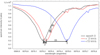 |
Fig. 1 Principle of shift-finding algorithm of Pierre Connes. Example of a spectral line at three epochs. Epoch 0 – reference (black), Epoch 1 – shifted by +2 km s−1 (red), Epoch 2 – shifted by +15 km s−1 (blue). The intensity change is measured within the dλ slice. This figure is similar to Fig. 4 in Connes (1985). |
3 The Cross-Correlation Function (CCF) algorithm to determine a radial velocity RV
Baranne et al. (1996) designed the spectrometer ELODIE, partially inspired by the work of Connes (1985), and stimulated by Michel Mayor. ELODIE is a cross-dispersed spectrometer and CCD. Installed at Observatoire de Haute Provence, it allowed the rapid discovery of 51 Pegasi b, the first exo-planet found around a Sun-like star, detected by the RV indirect method (Mayor & Queloz 1995). Earlier on, planets had been detected around a pulsar (Wolszczan & Frail 1992).
In Baranne et al. (1996), there is a description of the CCF algorithm applied to the series of stellar lines. The stellar spectrum intensity is digitized on pixels, each with an assigned wavelength. A box-car shaped “emission” line is 0 everywhere, and 1 in a small wavelength interval (for instance one pixel) centered on the absolute wavelength chosen for the transition responsible for the stellar line. The correlation function is computed on a fixed grid of potential absolute RV values (in km s−1). Each point of the CCF is the portion of the stellar spectrum which is included in the box-car. Usually the CCF is fitted by a Gaussian, and the wavelength of the Gaussian minimum reveals a “proxy” of the dynamical absolute radial velocity of the star. A series of emission lines constitutes a Binary Mask. Piling-up together all individual CCFs of one optical Echelle order of the spectrometer, to get one single CCF per order has the great advantage to average out some artifacts, for example pixel-to-pixel response nonuniformity (PRNU); optical fringes caused by the optics of the spectrometer, imprinted on the observed spectrum; and the blaze effect, which results in a bias when the CCF on one single line is fitted by a Gaussian.
In a word, the piled-up CCF algorithm is quite robust to several artifacts. Any pattern which is fixed in the wavelength frame of the spectrometer, while the star spectrum is moving by up to ±30 km s−1, will be detrimental (producing a bias on RV) for all methods which compare directly the motion of the spectrum, as the shift-finding algorithm or others, like template matching . This is the case of several artifacts (e.g., PRNU, dark current nonuniformity, DCNU), optical fringes, and micro-tellurics (large tellurics are just avoided by standard Binary Masks). For template matching, when the template is built from many observations with full yearly excursion of BERV, it will somewhat smooth out artifacts. Also, for CCF building some weights are usually assigned to each line of the Binary Mask (Pepe et al. 2002). For instance, Lafarga et al. (2020) use as a weight for each line the ratio between the contrast and the width of the line, where the contrast is the relative depth of the line and is given for each line of the official ESPRESSO BM. Then, all orders are combined together through the optimal combination of Gaussian errors, with a weight equal to 1/σord2. The uncertainty estimate for this order σord is given by the second formula of Connes applied to the CCF, as described in Boisse et al. 2010. Another way to combine the CCFs from all Echelle orders is just to add them together to get a single CCFtot per exposure, since each of the order CCF has been obtained from the addition of all CCFs of the BM lines inside this order, already weighted for each line. This is indeed the case of the official ESO/ESPRESSO pipeline at VLT. While a good pipeline is supposed to correct many artifacts quoted above (PRNU, DCNU, optical fringes, micro-tellurics, stray light, etc.), one should still worry about the residuals after the correction of these effects by the pipeline. Artigau et al. (2022) have improved the RV data by eliminating outliers (resulting from residuals after pipeline corrections) with a Line-by-Line analysis of Barnard’s star acquired with SPIRou spectrometer at CFHT.
4 Proposed algorithm: applying the first formula of Connes to piled-up CCFs
4.1 Description of the new EPiCA algorithm
We propose to combine the optimal retrieval, photon noise limited, algorithm of Connes Eq. (8) with the robustness of the piled-up CCF. We call it the “CF1 to CCF” algorithm (CF1, Connes formula 1) or the EPiCA method. Instead of applying the 1st formula of Connes to a measured spectrum at two epochs, we apply it to the two CCFtot computed for those two epochs, yielding CCF1 and CCF2. The trick is that the CCF is not computed on the wavelength scale provided by the laboratory calibrated spectrometer, but on the wavelength scale produced after correction from the barycentric Earth radial velocity (BERV). In the Solar System barycentric frame of reference, the radial velocity of a star is constant, except for the small variations induced by the potential presence of exo-planets. Today, conversions from geocentric to barycentric velocities have reached accuracy on the order of cm s−1 (Wright & Eastman 2014) and are not a limiting factor. Therefore, there is only a small displacement of the two curves CCF1 and CCF2, suitable to use the Pierre Connes algorithm (Eq. (1)) valid for small displacements. To the best of our knowledge, this method has never been used or described before.
In practice, in the CCF fits files taken from the ESO archive the CCF matrix has 171 columns, while there are only 170 Echelle optical orders. The last column of the CCF matrix is an order-merged CCFtot produced by the pipeline itself. We have verified that this CCFtot is computed by adding together all CCF per order for the exposure. We applied the EPiCA algorithm to this order-merged CCFtot of the pipeline (last column numbered 170 in the code, where numbering starts at zero). One particular exposure spectrum 1 is taken as a reference, providing CCF1tot. Each other exposure 2 provides a CCF2tot, and the 1st formula of Connes (Eq. (8)) is applied, yielding the change of RV, DRV, between exposure 1 and exposure 2. The CCF2tot must be normalized to CCF1tot before applying Eq. (8) (both CCF1tot and CCF2tot must have the same integral). However, we note that all computations required for Eq. (8) use CCF2tot before its normalization to compute the weighting function W(i) and the quality factor Q (the “on the fly” quality factor and Wi for each exposure).
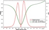 |
Fig. 2 Illustration of the simulation used to validate the Connes shift-finding algorithm and the error estimate. Black: CCF of original data (CCF1, right scale); green: CCF of simulated exposure shifted from original data (CCF2, left scale); red: weight function (left scale). |
4.2 Validation: simulation of shift-finding algorithm applied to an observed CCF
Here, we are testing the 1st and 2nd formulae of Connes (Eqs. (8) and (9)), applied to an observed CCF. For this simulation, we have used a series of 200 exposures on star HD 403074 taken during the night from 24 to 25 December, 2018 (called night 24 elsewhere in this paper). We have added all 200 spectra together, spectel to spectel, for order 104, and computed the CCFs on a given grid Vrad of radial velocities (Fig. 2, black curve). The S/N for one spectel is about 1000 for this reference spectrum S1. The wavelength scale WS1 was the spectrometer wavelength scale for exposure number 100. Order 104 (covering wavelength range 5523.8–5606.7Å) was selected because this order is not affected by tellurics, and the signal is rather high with one single exposure. The S/N for one point of the CCF is about 4000.
Then, a synthetic spectrum S2 was derived from the stacked spectrum S1 just by modifying the wavelength scale, as if the star had changed its velocity by +100 m s−1: same intensities but on a RV shifted scale WS2.
In order to mimic what would be the values of spectrum S2 sampled on the grid WS1, we interpolate the spectrum S2 vs. WS2 on all the points of the grid WS1. The CCF2 of the spectrum S2 sampled on WS1 is done on the same grid Vrad of radial velocities, yielding the green CCF curve of Fig. 2.
Also displayed in Fig. 2 (in red) is the weight attached to each point of the Vrad grid (Eq. 8), according to the photon noise limit of Pierre Connes first formula, here applied to the CCF1. The double-peak shape of the weight curve (in red) just shows the relative contribution (weight) of each point of the CCF to determine a shift: the weight is depending on the square of the derivative (with respect to the Vrad grid):
 (12)
(12)
When the first formula of Connes is applied to the CCF1 and CCF2, a radial velocity change DRV of 99.613 m s−1 is returned, while the second formula of Connes giving the uncertainty applied to CCF1 (or CCF2) is 0.366 m s−1. The retrieved DRV is near the + 100 m s−1 simulated RV shift, with a difference from 100 m s−1 near the nominal error bar. Therefore, this simulation exercise validates this new algorithm, and the uncertainty associated with it. It can be pointed out that, while applying a shift-finding algorithm to the comparison of spectra as a function of wavelength includes an approximation (finding a shift instead of a stretch), applying the same shift-finding algorithm to a CCF does not imply the same approximation, because the scale of the CCF is a radial velocity, and computing the CCF accounts exactly for the Doppler stretching.
4.3 Basic differences between the two RV retrieval algorithms
The ESO/ESPRESSO pipeline algorithm for RV retrieval is to fit the curve CCFtot (similar to green and black curves in Fig. 2) by a symmetric Gaussian and assign as absolute RV value the position of the center of the Gaussian. Therefore, only one single information is derived from the full CCFtot curve. Actually, as shown by González Hernández et al. (2020) for the Sun (integrated disk through observation of the Moon), the exact position of this symmetry axis of a Gaussian fit to a single solar line depends somewhat on the wavelength extent of the fitting domain, which shows that the spectral lines are not rigorously symmetric. Inasmuch as the curve CCFtot is an average image of all piled-up solar lines of the Binary Mask, it is likely that such a dependence also exists for the CCFtot. Then, RV changes of a star are just computed by subtracting a constant from all RV measurements.
On the other hand, the Connes algorithm does not claim to determine an absolute value of RV for each spectrum and corresponding CCFtot, but only the change DRV of RV between two spectra and their corresponding CCFtot. Actually, each point of the CCFtot gives an estimate of DRV, which can be combined together in an optimal way (mathematically) by applying the weight function of Eq. (12) (red curve of Fig. 2). This is what we have done in the following. However, there is potentially the possibility to study separately various parts of the spectral lines (or their image trough the CCFtot). In particular, the red side and the blue side could give different estimates of the RV change, if stellar activity deforms the spectral lines and CCFtot in a nonsymmetrical way. In summary, it is clear that the ESO pipeline for ESPRESSO must give, for each observed spectrum, one single number, an estimate of the absolute radial velocity of the star (in the barycentric system), revealed by its Doppler effect; and this is indeed what is provided by the present version of the ESO ESPRESSO pipeline when fitting CCFtot by a symmetric Gaussian.
When a change of RV between two spectra (taken at two epochs) must be evaluated, the simplest method consists of comparing RV1 and RV2 from the pipeline, and this is exactly what is done routinely during the search for exoplanets by most of scientific teams. However, the two spectra contain an enormous amount of information: they could be compared, in the extreme limit, spectel by spectel, with the Pierre Connes approach, each spectel giving an estimate of the DRV= RV2–RV1. This could be a way to detect some spectral regions which are affected by stellar processes changing the shape of the spectral lines (including variations of convective Granulation Blue Shift, GBS). Unfortunately, there are some artifacts spoiling this extreme approach: PRNU, DCNU not perfectly known and accounted for; optical fringes, which may change with the orientation of the telescope; uncorrected micro tellurics, to name a few. These outliers are well detected by the Artigau et al. (2022) technique which explains its success in increasing the accuracy of RV. On the other hand, using CCF order-by-order and even CCFtot, mitigates these artifacts by averaging them out: the CCF method is quite robust. With the proposed EPiCA method (applying the Connes approach to the CCFtot), there is a hope to combine the robustness of the CCF approach (which combines many lines together, and partially smoothes out some artifacts) and the sophistication of the Pierre Connes’ approach.
We note two other interesting studies that are using also CCFtot, with the aim (the same aim as us) to try to discriminate planetary reflex Doppler shifts from stellar variability. Simola et al. (2019) are adding one more parameter in the Gaussian fit to the CCF, the skewness (asymmetry). Collier Cameron et al. (2021) use the autocorrelation function (ACF) and departures from an average of all ACF, which requires a lot of observations. Here, we explore an alternate route, by studying in detail how the CCFtot behaves, with the help of the Pierre Connes shift-finding algorithm and the full details provided by the DRV curves.
5 Application to HD 40307 ESPRESSO data and three-planet model
5.1 Overview
Ideally, in order to compare two methods yielding changes of RV, one should use a planet-less star with a constant RV, and compute the standard deviation of a series of measurements of RV changes around the mean which should be 0. On the other hand, we wished to use ESPRESSO data which provide an absolute wavelength scale of excellent quality (Pepe et al. 2021), possibly the best in the world, and extensive series of measurements. Looking at the available ESPRESSO data, we noticed a quite exceptional series of 1151 exposures spread over 7 days of star HD 40307. HD 40307 is a K2.5V type star with visual magnitude 7.147 and distance 13 parsec. It was observed during 6 nights from 22 December to 28 December 2018 by ESPRESSO. The series of exposures were made in HR mode which resolution varies between 100 000 and 160 000 across the spectrum. It had originally be planned to search for an asteroseismology signal (finally, not found yet on this star), but has the advantage of providing a unique way to get an estimate of the true error made on RV changes, based directly from data on the dispersion of RV change residuals to a linear best fit during a short period of time. For this asteroseismological campaign5, the exposure time was set to 30 s for all 1151 exposures, and the sampling period was about 78 s.
The star HD 40307 harbors a multi-planetary system. It was reported by Mayor et al. (2009) that it hosts 3 super-Earth-type planets, with orbital periods Pb = 4.311 days, Pc = 9.6 days and Pd = 20.5 days. Later, Tuomi et al. (2013) independently analyzed HARPS publicly available data and concluded to the presence of 3 additional exoplanets with periods: Pe =34.62 days, Pf = 51.76 and Pg = 197.8. Díaz et al. (2016) confirmed the three planets found by Mayor et al. (2009) and planet f from Tuomi et al. (2013), but cast doubt on the presence of planets e and g. The most recent analysis made by Coffinet et al. (2019) confirm the findings of Díaz et al. (2016): they found 3 exoplanets from Mayor et al. (2009) and also the additional planet f from Tuomi et al. (2013), but as well as Díaz et al. (2016) cast doubt on the presence of planets e and g. After subtraction of a long-term signal, which probably represents a magnetic cycle of the star, the signal around the period of 200 days has a very low significance and the signal around 34.6 days is absent.
In our analysis, we considered only the three planets b, c, d, and excluded planet f, because its period of 51.76 days is considerably longer than the short duration (7 days) of the time series and would not make any significant difference in a model fit to data.
5.2 Comparison of the two RV time series obtained with the two methods
We now compare the two RV time series: the official ESPRESSO, containing the RV assigned to each exposure recording one spectrum of HD 40307 (the pipeline series), and the time series that we obtained from our new EPiCA method, CF1 applied to CCFtot. They are plotted in Fig. 3, not as a function of time, but as a function of exposure number; the data are concatenated. From the pipeline RV data was subtracted a constant radial velocity of 31.3668 km s−1, while the EPiCA series displays the RV change between each exposure and exposure no10 taken as an arbitrary reference. Therefore, the overall offset between the two time series is arbitrary and has no particular significance.
Both time series show a rather sharp decrease after exposure 615, which is the last one of the night 25 (in short for 25 December). This is due to the presence of planets, as we shall see later. The offset between the two series is partially due to the difference of reference exposure: n°0 for ESPRESSO pipeline, n° 10 (first of night 24) for Connes CF1 applied to CCFtot. But the offset is not constant, as can be seen when plotting the difference between the two time series (Fig. 3). There is a change of ≃1.3 m s−1 between nights 25 and 26.
Therefore, one of the two methods is giving some wrong results by about 1.3 m s−1 (or may be both of them), which do not correspond to a true change of the dynamical radial velocity dR/dt. We suspect that this is the effect of stellar processes, and more precisely of granulation blueshift (GBS) changes, on a timescale of a few hours, together with the fact that both methods are differently sensitive to stellar processes.
5.3 Comparison of RV dispersion over one night from a linear fit
One criterion for RV retrieval method comparison is the use of a time series of measurements when the star is not moving at all. The precision of the RV method is quantified by the mean error, equal to the standard deviation σ (the square root of the variance) of the series of measurements (this is the definition of the precision). In our case of the HD 40307 time series, the star is moving because of planets, and RV is changing. However, we may restrict the time series to a particular night and a limited duration in such a way that the RV variation is small and close to linear. In this configuration, we may accommodate with planet-induced star motion by subtracting a linear fit and computing the standard deviation of the residuals, as a quality indicator of the method. Actually, this linear fit may also include spurious RV variations due to stellar variability affecting the Doppler shift of the disk-integrated spectrum.
The first night contains only 10 measurements and is not suitable for this statistical exercise. The third night (25 December) displays a significant number of outliers, affecting the second half of the 200 measurements (Fig. 3). This behavior has been assigned to an instability of the cooling system of the ESPRESSO blue detector (Figueira et al. 2021). Therefore, the night of 24 December containing 406 measurements was selected for further comparison of the two methods.
As said above, we compare in Fig. 3 the EPiCA results with the results from (symmetric) Gaussian fits to CCFtot (the RVs from the pipeline). Although not easily visible by eye, there is a gain (i.e., a reduction) in RV dispersion σ in the case of the EPiCA method. The cloud of data points can be seen on Figs 4 and 5 at night 24 and day 2.2.
In order to compare quantitatively the two methods we made a linear fit to the 406 values of RVs of night December 24th for both measurement methods and removed a linear trend (due to planets and/or stellar processes) to keep only the residuals, and compute the dispersion around the average value. We made two histograms of the residual RV values with the same bins and compared them, as shown in Fig. 6. The figure clearly shows the gain in precision with the EPiCA method, quantified by the widths of Gaussian fits to the two histograms. For this series of exposures, the semi-width of the Gaussian (at 1/e) is reduced with the EPiCA method with respect to the pipeline, from 1.46 to 1.17 m s−1, corresponding to a reduction of the dispersion (the actual mean error on RV changes measurements) from σ = 1.03 to 0.83 m s−1, a significant 20% improvement of the precision.
The result is not very surprising, since P. Connes demonstrated that his first formula is the optimal way to measure Doppler shifts, by taking into account the totality of information contained in the two spectra (or here, the CCFtot). On the other hand, as we discuss below, the hypothesis underlying the Connes formulation is an absence of variability of the shape of the spectra (or here CCFtot), except for a single shift. Only pure Doppler shifts are allowed. We interpret this decrease in the RV dispersion during a short duration as evidence for the absence of strong variations of the stellar line shapes, at least of the absence of shape variations strong enough to cancel the benefit of the application of the CF1 formulation.
5.4 A three-planet best fit to the official pipeline ESPRESSO RV time series
We now examine a second quality indicator of an RV changes retrieval method, totally independent of the first one, namely the true error computed from dispersion, discussed in the previous section. Our goal is to investigate whether or not the EPiCA method may be less sensitive than the Gaussian fit to spurious changes of RV due to stellar activity. The idea is that the RV changes due to planets do obey strictly to Kepler’s laws, while RV changes due to stellar activity are more random (but still stochastic, Meunier 2021; Meunier et al. 2023). Therefore, we may produce a quality indicator indicating how well a series of measurements reproduce a pure Kepler’s law model of RV changes. To do so, we have used the entire HD 40307 time series. For each method, we have determined some best-fit parameters of the three-planet system, and computed the absolute difference between data and best-fit model as the second quality indicator. In Table 1 we summarize some parameters of the three planets detected around HD 40307.
 |
Fig. 3 Two RV time-series and their difference. Top: comparison between the RVs derived from the Gaussian fit and the EPiCA method. The data (RV changes in m s−1) are plotted as a function of exposure number. The pipeline RVs are plotted with their error bars, in a different color for each night. They were derived by subtracting from all pipeline RV data contained in each spectrum fits file the value of the first exposure: 31.3668 km s−1. Red points are obtained by the EPiCA method applied to the CCFs of the current exposure and the first exposure of night 24 (exposure n°10 when all nights are concatenated), taken as a reference. A constant 2 m s−1 was subtracted for clarity. Bottom: differences between the two time series of RV changes: Gaussian fit – EPiCA (CF1 applied to CCFtot). This difference shows an abrupt decrease (~1.3 ms−1) after exposure no. 615, corresponding to the transition from night 25 to night 26, which remains after that. |
5.4.1 Best-fit strategy and result of RV official pipeline ESPRESSO RV time series
Our first analysis is done only on ESPRESSO 2018 data, without archive HARPS data. ESPRESSO data set consists only of 6 days, so it is not possible to detect a signal from the 4th (HD 40307 f), since it would induce only a too small drift over 6 days. We have assumed that planets are on circular orbits as it is mentioned in Table 9 from Díaz et al. (2016).
Therefore, we kept fixed the amplitudes and periods of three planets at their most recently published values from Coffinet et al. (2019), where the authors corrected the HARPS wavelength calibration from the CCD stitching, a gap in blocks of pixels composing the full CCD. We know the time T0, the origin of the sinusoidal wave at epoch 2008 from the exoplanet.eu (see Table 1). With these time values of ascending zero crossing in March-April 2008, we can extrapolate in time all 3 sine waves with the defined periods up to the epoch of 2018 observations, getting the curve RVnominal (pale gray, thick solid line) in Fig. 4, compared to ESPRESSO data. We see a major discrepancy, easily explained: an error on any of the periods, propagated over 10 yr, will make RVnominal not representing well the data of 2018. Also represented with a dashed gray line is the extrapolation with a period of planet b shorter by 0.0004 day, twice the claimed error bar. We are still far away from a reasonable fit.
Therefore, we have to adjust the exact times of ascending zero crossing near the time of observations, for each of the sine functions in order to get a good fit of data. Actually, we take as unknown in the fitting process the exact phase of each of the sine function at a reference time (BJDref = 2 458 474.5), taken as the time 0 of the plot of Figs 4–11. It is adjusted by a classical Levenberg-Marquardt scheme within IGOR software. We also have to let free a constant offset parameter w0, added to the three sine functions, since we deal only with variations of RV.
In Fig. 5 is plotted the best-fit curve, in black, while the three sine waves for the three planets are represented by dashed lines around the zero line. It is clear that the drop in RV between night 25 (day 3.2) and the next night 26 is mainly due to planet b, with smaller contributions from planets c and d.
Characteristics of three planets in the HD 40307 system from the HARPS 2008 campaign (Coffinet et al. 2019).
 |
Fig. 4 Comparison of pipeline RV time series with three-planets modeling. The black dots represent the time series of changes of RV values contained in the official pipeline, obtained by subtracting the RV value of the first exposure of the first night. The thick pale gray solid line is the extrapolation of the sum of the three sine waves as determined from 2008 HARPS data. It does not closely fit the data because the extrapolation over 9 yr is sensitive to small errors in the periods. The dashed gray lines is the same as the solid gray line, but with planet b period shorter by 0.0004 day, corresponding to twice the claimed error bar for the period of planet b. The solid black line is the best fit to the pipeline RV data by adjusting the phases of the three planets. |
5.4.2 Refining the periods by comparing 2008 and 2018 data
For each of the sine curves, knowing the phase at BJDref then allows us to compute the time T2b (respectively T2c, T2d) of start of the period (sin = 0 and becoming positive) just before BJDref. The values are displayed in Table B.1 with their uncertainties.
We find in the literature that a similar sinus = 0 crossing happened for planet b at T0b = 2 454 562.77 ± 0.08 BJD, on April 5, 2008. Therefore, we may determine a precise value of the average orbital period of planet b between epochs April 2008 and December 2018, knowing that it must be an integer number of periods between T0b and T2b. The elapsed time difference T2b – T0b=3909.0964±0.088 days. Here we take as the uncertainty the quadratic sum of the two uncertainties, respectively 0.08 and 0.037 days for T0b and T2b. Dividing the elapsed time difference by the nominal period 4.3114 gives a number of orbits of planet b Kper=906.688 (Table 4), while it should be an integer number. We designate by K1 and K2 = K1+1 the two integer numbers encompassing Kper.
With 907 full orbits between T0b and T2b, the period is found to be Pb907 = 4.30992±1.0×10⁻⁴ days, while with 906 full orbits, the period is Pb906 = 4.31467±1.0×10⁻⁴ days (Table B.1). These two values encompass the original value of the period found at discovery announcement 4.3115±0.0006 and the more recent value Perb=4.3114±0.0002. Therefore, we favor the Pb907 which is about 2.2 times nearer this value Perb=4.3114 than Pb906. Still, this new accurate value Pb907 is different from the nominal 2008 period Perb = 4.3114±0.0002 by 0.0015 day, outside the claimed error bar errPerb = 0.0002 by a factor of 7. The planet b may have changed its average period from interactions with other planets between 2008 and 2018. Alternately, the uncertainty of 0.0002 day claimed for 2008 data was underestimated, but some arguments developed in Appendix B suggests that this is unlikely the case. Actually, similar results are found with both methods applied to 2018 observations, Gaussian fit (pipeline) or EPiCA (see next section). This is a potentially very interesting result, because it could reveal the influence of other planets on the orbit of planet b. However, since it is irrelevant to the comparison between the two RV methods, we defer this subject to Appendix B for further discussion.
The same procedure was done for planets c and d, and the results are in Tables B.2 and B.3 respectively. Clearly, Kper is nearer an integer number than for planet b, and the most likely values are Kper = 407 for planet c, and Kper = 193 for planet d.
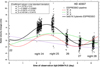 |
Fig. 5 Same as Fig. 4, but with individual contributions of the planets. The three-planet best-fit curve is in black (solid line), while the dashed lines are each of the three sine waves representing the three planets: b (red), c (green), d (violet). The best-fit curve is the sum of the three planets plus a constant w0 = 1.5576 ± 0.515 m s−1. |
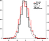 |
Fig. 6 Histograms of RVs from the two different time series. They are obtained for the 406 exposures of night Dec24, after removal of linear fits to each series. The histogram is in red for the Gaussian fit and in black for EPiCA. Gaussian widths of histograms are indicated for each method. The EPiCA histogram is narrower than the Gaussian fit histogram. |
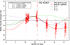 |
Fig. 7 Same as Fig. 5, but for the time series obtained with EPiCA (red dots). The first exposure was taken as the reference. The best-fit curve is in red (solid line), while the dashed lines are each of the three sine waves representing the three planets: b (black), c (green), d (violet). The best-fit curve is the sum of the three planets plus a constant w0= −2.2106 ± 0.726 m s−1. |
5.5 A three-planet best fit to the EPiCA derived time series
We want to find out if the use of EPiCA method (CF1 applied on CCFtot) is able to produce an improvement in the case of a planetary system. To do so, we applied exactly the same fitting methods as in Sect. 5.4.2, this time by replacing pipeline results by EPiCA results. Figure 7 illustrates the fit by a model with three planets to data computed by EPiCA method (CF1 on CCFtot).
In Fig. 8 are compared the best-fit curves for the three planets obtained with the two methods, pipeline and EPiCA. While there is not much difference for planet b, there is some substantial time shift for planets c and d.
The same exercise to compute the period from the elapsed time between two zero crossings (from negative to positive) of the sine wave was done for the best fit to RV data retrieved with EPiCA method. The results (also shown in Tables B.1, B.2, B.3) for the two methods are not very different. For planet b, and with the EPiCA method we find the same period offset as the nominal period found at 2008 epoch. We have summarized in Table 2 the new results of the periods of the three planets both for the best fit to pipeline data and EPiCA data. The results of both methods are similar. We have also indicated the difference of period between the nominal (old) value, and the new value found from the CF1 method. As mentioned above, this difference for planet b is 7.5 times larger than the previously claimed error bar. For planets c and d, the difference is 2.5 and 2 larger than the claimed error bar. In summary, joining the 2008 and 2018 data is providing more accurate periods than those which were determined with 2008 observations only, and this is valid for both methods.
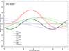 |
Fig. 8 Comparison of the best-fit models to the two time series. Solid lines are for the ESPRESSO pipeline. Dashed lines are for the EPiCA method. The red curve is for the total of three planets (+ the offset w0), while planets b, c, d have different colors. |
5.6 Comparison of the residuals to three-planet best fit between the two methods
In Fig. 9 are represented (black points) the residuals (δRV time series after subtraction of the best-fit model) for the RVs from the pipeline (Gaussian fit), and similarly (red points) in Fig. 10 the residuals for the EPiCA method. By eye, it seems that the EPiCA method is better aligned on the Zero line (solid black line) than for the δRV time series from the pipeline.
This visual impression is confirmed by the following statistical analysis, summarized in Table 3 and in Fig. 11. The first night (December 22) contained only 10 exposures, and is not in Table 3. The second night (24) is the longest one and contained 406 exposures. It shows the smallest standard deviation, quite similar for the two methods. The third night (200 exposures) had a specific problem. An instrumental noise due to a blue detector instability spoiled somewhat the second part of the night (visible on all figures with data, residuals, and standard deviation). This is why we computed the standard deviation and mean residual per night for both the first 100 exposures only and for the 200 exposures of the night, as two separate entries for night 25 in Table 3.
The mean nightly residual (which can be qualified as a bias varying from night to night) is significantly nearer zero for the EPiCA method than for the official pipeline. More precisely, the mean of the absolute value of the nightly averaged residuals of the five nights 24–28 (we exclude the first night 22 which has only 10 exposures) is 0.11 m s−1 for the EPiCA method instead of 0.32 m s−1 for the Gaussian fit. Similarly, the RMS of the five nightly averaged residuals is 0.13 m s−1 and 0.39 m s−1 respectively for the two methods. This is a measure of the quality of the fit to a three-planet Keplerian model: a factor of 3 in favor of the EPiCA method. In our mind it is a strong indication that this new method of applying CF1 to CCFtot is giving a result which is nearer the truth than the Gaussian fit. Admittedly, the factor 3 improvement of Kepler fit to a RV time series by using EPiCA method is tested on only one example, and is likely not representative of all RV time series collected so far. It should also be kept in mind that such low values, 0.11 m s−1, or even 0.32 m s−1, are anyway excellent, and reflects the high quality of ESPRESSO data, which is certainly even better after the upgrade of the blue detector cryostat in June 2022.
Characteristics of three planets in the HD 40307 system from the HARPS 2009 campaign.
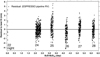 |
Fig. 9 Residuals after subtraction of the best-fit model from the δRV official Gaussian fit (black points). It seems by eye that the average of groups of points do not always lie on the zero line. There is a bias that depends on the day of observation (numbers represent the night of December 2018 when HD 40307 was observed.) |
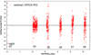 |
Fig. 10 Residuals after subtraction of the best-fit model from the CF1 to CCFtot time series (red points). It seems by eye better aligned on the Zero line (solid black line) than for the δRV time series of Fig. 9. |
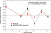 |
Fig. 11 Mean residual for each night as a function of time (BJD-BJDref). Black: Gaussian fit. Red: EPiCA method (CF1 on CCFtot). The error bars are computed as the standard deviation divided by sqrt(number of exposures). The two points for night 25 (around 3.2 days) are not independent. |
6 EPiCA method and detection of changes in the spectral shape of stellar lines
As detailed above, the EPiCA method provides, for each point i of the radial velocity grid used in the building of the CCFtot, an estimate of the change of radial velocity DRV(i), with an associated error bar, between two exposures at epochs E1 and E2. In previous sections we considered only the change of RV obtained by combining optimally the various values of DRV(i). However, it is also possible to examine the curve DRV(i) in detail, as a function of point i. If there is no change in the CCFtot shape between the two exposures, the DRV estimate should be constant across the RV grid. If it is not constant, then it means that the spectral lines shape have changed between the two epochs E1 and E2. Since CCFtot is an “image” combination of all spectral lines in the stellar spectrum, this change must reflect at least a physical effect that is dominating in the average “image” even if it is not present identically in all the spectral lines.
In order to increase the S/N (up to about 3000), we have stacked the CCFtot by 100 consecutive exposures whenever possible (taken over about 2 h), and a little less otherwise. Night 24 contains 406 exposures, and is divided in 4 periods. There are 200 exposures for night 25, thus divided in two periods; night 26 has 174 exposures, divided in two parts; same for night 27 with 176 exposures and night 28 with 185 exposures. Hereafter we name for night XX and first (resp. second) series of exposures by C-XX-1 (resp. C-XX-2). Before any computation of a ratio, the two curves were normalized to each other, to account for photometric changes and to get a value around 1 at the extremities of the curves, corresponding to the shoulders of CCFtot.
Changes in the spectral shapes can also be detected directly by dividing a CCF of one exposure by the one of a different exposure. This can be done also using CCFs averaged over several exposures. In this section, we have taken advantage of the unique series of short exposures to explore the application of EPiCA for this purpose and to compare with divisions. We explain why the diagnostic using EPiCA is easier to perform.
Doing this study, we found a small change of the spectral shape during the first 2 h of exposures (about 100 exposures, first quarter of night 24 and half of the total observation period for nights 25, 26, 27, 28), a change similar for all five nights, and diagnosed with both CCF ratios and with EPiCA. Because of this systematic, repetitive behavior and the similarity of shape variations for the five nights, we separated their study from the study of the other types of spectral shape variability. The former effect is described in the first part of this section, and, in order to avoid the inclusion of its type of variability, we restricted the analyses presented in the second section to comparisons between either the two first parts, or the two second parts of the nights.
Statistics per night on standard deviation and mean residual, both in m s−1.
6.1 Change of spectral shape between the first and subsequent periods of time within the same night
6.1.1 Using CCF ratios
If there is a simple shift between two curves CCF1 and CCF2, their ratio should present a characteristic shape displayed as smooth colored curves on Fig. 12 (top), the results of a simulation using the curve C-24-1 (first stack of night 24) and shifting it by –20, –10, –5, +5 m s−1. By comparison, the computed ratio C-24-2/C-24-1 (after normalization) is characterized by a centered bump, quite different from any of the model curves. The ratio curves C-24-3/C-24-1 and C-24-4/C-24-1 are very similar to the ratio curve C-24-2/C-24-1, showing that the shape of C-24-3 and C-24-4 are very similar to the shape of C-24-2 : the variation producing the bump occurred only between the first and second parts of the night 24, and the shape did not change afterwards during this night 24. This is confirmed by the ratios between part 2 and 3, and also part 3 and 4 of night 24, displayed in Fig. 12 (bottom panel), which are constant within the fluctuation level observed for all ratios. Actually, we found out a similar central bump (and thus systematic behavior) when making the ratios of second part to first part of the night C-XX-2/C-XX-1 for the other nights XX = 24 to 28, as shown in Fig. 12 (bottom), with the central bump increasing from day to day. Such a centered bump in the ratios of CCF is the signature that the so-called contrast (relative depth) is decreasing with time between the two CCF. A change of contrast is often used classically as a stellar activity indicator. This is quite possibly the case here for HD 40307. However, in the present case, because of the somewhat systematic behavior of contrast change along each night of observation on a timescale of ≃2 h, we cannot completely exclude that this effect is connected to an artifact of so far unidentified origin.
6.1.2 Using EPiCA
In this subsection, we examine how the change of contrast along a night revealed by the ratios of CCF of the previous section translates into the shape of DRV(i) curves derived from EPiCA. Figure 13 displays several profiles along the velocity grid DRV(i) obtained with EPiCA for pairs of the same types of time periods as used in the previous analysis based on CCF ratios. For this figure, the two members of each pair belong to the same night. Error bars are computed for each pair based on the second Connes formula (Eq. (9)) and reflect the weights associated with the slope of the CCF. A typical series of weights is superimposed. The two most central values suffer from the division by the very small derivative (Eq. (3)) and additional uncertainties due to BM coarse velocity sampling (500 m s−1) and the corresponding area is marked by a rectangle.
In the case of a pure Doppler shift (i.e., in the absence of a change in stellar line spectral shape), the DRV(i) curve should be flat. This is indeed the case (see top of Fig. 13) for the two DRV(i) profiles for night 24 which are inter-comparing the second and third, then third and fourth parts. They are flat, within the error bars: there is no change of contrast, as revealed by the ratios of curves in Fig. 12 (bottom); the instrument has stabilized. On the contrary, the other DRV(i) curves of Fig. 13 depart significantly from a flat, constant, value. For all pairs of periods containing the first and second parts of the night, the profiles exhibit departures from zero on both sides of the central velocity. Moreover, the amplitude of these features increases from night 24 to night 28, forming extended spikes. Also, there is a difference of average level between the two sides of the curve DRV(i): it is positive on the blue side (≤31.4 km s−1), and negative on the red side. This is consistent with what is expected from the Connes algorithm applied to this particular case of change in shape (i.e., when the CCFtot becomes shallower) between stack 1 and stack 2 (decrease in contrast); the increase in intensity of the blue side is interpreted by the algorithm as a redshift, while the increase in intensity of the red side is interpreted as a blueshift. This case is similar to one of the model exercises performed by Cretignier et al. (2020), comparing the Gaussian fit of a spectral line with the algorithm of Connes, as we do here (their Fig. B3). Namely, it is the third row of their Fig. B3, where they model a decrease in depth (or contrast) induced by temperature-sensitive lines. All in all, both approaches (ratio curves and DRV(i) curves) are consistent, pointing to a small decrease in the contrast of CCF along each night.
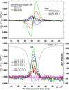 |
Fig. 12 Model-data comparison using CCF ratios. Top: expected ratio of two CCFs with unchanged shape and various Doppler shifts (colored lines), and ratios using the four periods of night 24 (black lines). The same curve is observed for ratios of parts 2, 3, and 4 to part 1. It does not resemble the expected variation for a simple shift and indicates a change in shape during the first and second parts of the night. Bottom: ratios of pairs formed by the first two consecutive stacked CCFtot obtained during the same night, for nights 24 to 28 (numbers indicated on the plot for 26 to 28). One CCFtot is drawn (gray line). There is a systematic bump centered on the CCFtot, indicative of an increase in signal near the center during the first and second parts of each daily pair. The increase is larger for the latest nights. The ratio for the two last parts of night 24 is shown for comparison (pink line). There is no increase in this case, a sign of absence of shape variation during this period. |
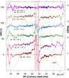 |
Fig. 13 EPiCA profiles DRV(i) along the velocity grid for pairs of time periods (lines with markers). Offsets of 30 m s−1 are applied between two consecutive profiles, except for the two top curves, which are plotted together. The actual zero value is indicated by a black thin line. The size of the markers is increasing with the individual weight for each series. A typical weight function is also plotted (thin dot-dashed line). The two most central values suffer from additional uncertainties due to the limited velocity sampling and are delimited by a rectangle. (Top curves) For pairs made of the second to fourth parts of night 24, the profiles are flat within the error bars, showing no significant change in shape; this is consistent with the constancy observed using ratios, pointing to a stabilization of the instrument. For each of the other pairs (lower curves) containing the first and second parts of a night, one can observe departures from a flat profile, and a similar shape with an amplitude increasing from night 24 to night 28. This typical shape of DRV(i) is induced by a decrease in contrast (see text), consistent with the same type of behavior as the bump measured using CCF ratios (Fig. 12). It could be due to a stellar process or to an artifact. |
6.2 Change of spectral shape between two consecutive nights
Whatever the cause of the observed change in contrast between the first part of the night (≃2 h or 100 exposures) and the rest of the same night, we have also studied the change of shape from one day to the next by comparing two stacked CCFtot taken similarly along each of the two nights (i.e., using pairs of type C-25-1/C-24-1, C-25-2/C-24-2, C-26-1/C-25-1, C-26-2/C-25-2, etcetera).
6.2.1 Using CCF ratios
The CCFtot ratios for two consecutive nights are displayed on Fig. 14. There are two curves for each couple of days, one for the pair of first CCFtot of the nights, one for the pair of second CCFtot of the nights. The two curves for pairs of the same two nights are very similar, even in their detailed structure, in spite of the fact that they are built from different, and fully independent data sets, bringing some confidence in their credibility. The curves are different from day to day. The ratios are close to constant, except for the pairs 25/26, which are characterized by positive and negative values far above the noise. This large change between the two nights (quantified by the standard deviation over 81 points of the ratio) happens at the time of the largest RV change (≃–4 m s−1) predicted by the planetary model (Fig. 4), but, of interest here, also at the time of the abrupt change (by ≃–1.3 m s−1, Fig. 3) of the difference between the two time series, Gaussian fit to CCFtot and EPiCA method. Importantly, the change of shape of the ratio observed from day 25 to day 26 is quite different from the model prediction for a simple shift (see a model for a shift of –5 m s−1 superimposed for comparison in Fig. 14). This observed departure from a pure Doppler shift clearly indicates a significant change of spectral shape between night 25 and night 26, quantified by sdev= 8.3×10⁻⁴. The other night ratios show smaller changes, quantified (in decreasing order) by sdev = 5.6×10⁻⁴ (27/26), 4.7 ×10⁻⁴ (25/24), 4.4×10⁻⁴ (28/27). The ratios for pairs of the same night 24, 24-4/24-3 and 24-3/24-2 have a sdev=1.9×10⁻⁴, representative of the noise level for such ratios. The two red and black curves of 27/26, and also the ones of 28/27 ratios are different from each other near the center, because of the contrast artifact which is more severe for nights 27 and 28 than for the previous nights, as shown in Fig. 12 (bottom).
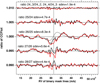 |
Fig. 14 Ratios of pairs of CCFtot taken one day apart along the HD 40307 campaign. They are plotted as a function of RV(i), the abscissae of the CCF. There are two pairs for each couple of consecutive nights. The ratios are vertically displaced by multiples of 0.005 for each pair for clarity. The first and second pair of the night are respectively in red and in black. The standard deviation of the curve is indicated. The upper curves are two ratios of night 24, whose wiggles are small and likely representative of the noise level for all curves. There is a marked departure from flatness for the ratio 26/25, as expected from the Kepler fit RV drop between nights 25 and 26. However, the observed ratio is very different from a model ratio in the case of a pure Doppler shift, as can be seen from the comparison with the superimposed model for a pure shift of –5 m s−1 (gray curve). Therefore, this set of curves indicates directly a change in shape between the two nights. |
6.2.2 Using EPiCA
Similar to the previous section using the CCF ratios, we searched for changes of spectral shape from one night to the other using EPiCA and the same parts of the night. Figure 15 shows the results separately for each pair of consecutive nights. The two series of profiles, using the first or the second time periods of the two consecutive nights, are very similar, despite being derived from independent data sets, in the same way CCF ratios were similar. The DRV curves for the pairs of nights 24–25, 26–27 and 27–28 show somewhat constant values near 0 for both the blue and red sides (still restricting to the data points with low error). This is consistent with a pure, very small Doppler shift. In the case of the two DRV curves between night 25 and 26, their shape is very different from the other DRV curves, and, clearly, these DRV curves of the pair 25–26 stand alone. One would expect a flat profile at about –4 m s−1 in both the blue and red side, according to the planetary model. However, the two sides of the curves are very different from each other. The blue side is negative, which is consistent with the planetary motion between day 25 and 26 (Fig. 4), but decreases strongly below –4 m s−1; we discarded from the discussion the two spikes near the center. The red side is also not constant, and decreases but is globally positive. Such behavior is showing that the shape of the CCFtot profile has changed substantially between night 25 and night 26. This is totally in line with the change of shape characterized by the ratios of CCFtot displayed in Fig. 14, where also the pairs of ratios between nights 25 and 26 stand alone among one day apart ratios, with a pronounced change of shape, not symmetrical with the center of the line.
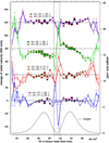 |
Fig. 15 Same as Fig. 13, for four pairs of stacks that are one day apart over the five nights from night 24 to 28. Each pair consists of using either the first or the second parts of night. Offsets of 40 m s−1 are applied between two pairs of these EPiCA profiles. The actual zero value is indicated by a black thin line. The DRV curve for the pair 25–26 shows a different pattern in comparison with the other pairs, with a strong difference between the blue side and the red side. |
6.3 Conclusion about the line shape variations and the two methods of detection
In summary, we found that the DRV(i), the Doppler velocity shift between two CCFtot is sometimes very far from being constant along the RV grid points i. This is the proof that the spectral lines are changing their shape, in addition to any Doppler shift, on a timescale of ≃2 h or a little shorter. With the help of the ratio curves, we detected a somewhat systematic effect: a central “bump” builds up between the first stack of the night, and the second stack, along each of the five nights, possibly of stellar origin or resulting from an artifact. Whatever its origin is, we mitigate this effect by comparing CCFtot taken at the same relative time during the nightly operation and one day apart. Doing so, we detected a significant variation of shape, between night 25 and night 26, exactly at the time of the abrupt change of the difference between the RV time series deduced from the Gaussian fit and the EPiCA method (decrease by ≃1.3 m s−1). This suggests that the change of shape modifies differently the results of the Gaussian fit and the shift-finding algorithm. We assign this change of shape to the stellar activity.
For both types of detection, it is interesting to compare with the lineshape simulations of Cretignier et al. (2020) displayed in their Fig. B3. First, the authors conclude that, adding a symmetric perturbation to a symmetric spectral line, both methods, Gaussian fit and Connes’s formalism (equivalent to EPiCA) are robust, and the retrieved RV does not change. On the contrary, if a symmetric perturbation to a nonsymmetric line (which happens at least whenever there is a blend of a smaller line on one side of the line), then both algorithms are retrieving a somewhat biased change of RV. The “bump” centered described in 6.1.1 resembles a case of a symmetric perturbation, such as a change of contrast. It is very likely that a fraction of lines from the binary mask has blends. But since secondary line blends are distributed at random, the CCFtot will be much more symmetric than a single blended line, and it is likely that both methods are robust to this artifact, yielding small biases if any. The case of the addition of a nonsymmetric perturbation is not shown in their exercise, but, from their exercises of addition of a symmetric perturbation, we certainly may expect that a biased DRV will be retrieved for both methods. Actually, the (largest) change of shape observed from night 25 to night 26 is strongly asymmetric (Fig. 15), and therefore we may expect that the DRV retrieved by the two methods will both be biased erroneously away from the true dynamical change of RV due to planets. Because this peculiar behavior between night 25 and 26 corresponds exactly to the abrupt change of the difference between the two time series (drop by ≃1.3 m s−1), the classical Gaussian fit and the EPiCA method, as displayed in Fig. 3, this difference in the time series of ≃ 1.3 m s−1 is certainly the difference of biases between the two methods.
Which method provides the smaller bias? Extensive simulations are beyond the scope of this paper. Whatever the answer, we may emphasize that EPiCA is a more direct and easier way to detect shape variations. Departures from flat DRV(i) curves are an easy diagnostic of shape variation, they cannot be confused with effects of a pure Doppler shift, and there is no need for a comparison with a model, as in the case of CCF ratios. We also argue that the EPiCA method is easier and has more flexibility in the analysis of departures from a single Doppler shift between two epochs than the comparison of CCF bisectors. By essence, the bisector is making a link between both sides of the spectral lines (or the CCF image), while the Connes algorithm is applied independently to each point of the line (or the CCF image). The bisector says nothing about the length of segment joining the two sides of the line: the center of the segment may not move, while the length of the segment may change without being noticed by the bisector analysis. One may oppose that in this case there is no bias in RV, but symmetric variations like those detected at the beginning of the observing periods would not be detected.
The variation of stellar line shape from night 25 to night 26 is likely a result of stochastic changes of the convective granulation blueshift (GBS) averaged over the stellar disk (Meunier & Lagrange 2020; Meunier 2021). Model results of these authors indicate an amplitude of RV Doppler shift fluctuations of ≃0.2 m s−1 for a star of K4 type (similar to HD 40307, type K2.5), when granulation only is considered on timescales of 15–50 min, and up to ≃1 m s−1 for super-granulation changes (on a ≃1 day timescale). Such a super-granulation change could explain the important departure from constancy of the DRV(i) curve, and the corresponding change by ≃1.3 m s−1 between the difference of RV retrieved either from the Gaussian fit or from EPiCA method, and remaining during the following nights 27 and 28.
7 Summary and discussion
In this paper, we described and tested a new way to estimate the change in radial velocity DRV between two epochs from the comparison of the two stellar spectra. This algorithm is based on the first formula of Pierre Connes; its aim is exactly this, and was shown to be the (mathematically) optimal way to retrieve DRV. Instead of applying the shift-finding algorithm to two spectra, as it was originally designed, or to individual spectral lines, as in some line-by-line techniques, it is applied here to the weighted sum of all CCFs obtained separately for each order, CCFtot, which represents an average image of all spectral stellar features. If the computation of CCFtot is done on a wavelength scale associated with the Solar System barycentric frame (i.e., using the corresponding barycentric velocity grid), the reflex motions induced by planets are small and one can stop at the first-order term of the Taylor expansion involved in the formalism of equation 2. This new EPiCA method is simple to implement and appropriate when pipeline data products of the spectrograph include CCFtot in the Solar System barycentric frame. It combines the advantage of the shift-finding algorithm and the robustness of CCF construction.
To test the algorithm, we used a series of spectra acquired during a one-week observing campaign on star HD 40307, which is known to host at least three planets, and we compared the two RV time series obtained from the CCFtot profiles by means of a Gaussian fit, on the one hand, and our new EPiCA algorithm, on the other hand. In order to compare quantitatively the two methods, two different quality indicators of the retrieved RV time series were computed.
First, a single-night series was examined. The RV series were fitted to a linear relationship representing the first-order Doppler variation under the influence of planets, but also any RV change that could be due to stellar activity. The first-order approach is justified by the short duration for the analysis. The dispersion of the residuals to the linear fit, which is a measure of the mean error, was found to be σ = 1.03 and 0.83 m s−1 respectively for the pipeline and the EPiCA algorithm, a significant 20% improvement of the precision on RV changes. We interpret this decrease in the RV dispersion as evidence for the absence of strong variations of the stellar line shapes during this time interval, at least for the absence of variations strong enough to cancel the benefit of the application of the Connes shift-finding algorithm which makes an optimal use of all the spectral information, but requires unchanged profiles.
In a second test, we made use of the whole series obtained over the campaign, and the computed RVs were fitted to a three-planet Keplerian model. The periods and reflex-amplitudes were fixed to the previously determined values, but the phases were adjusted. Based on the nightly averaged residuals to the respective best fits (Fig. 11), we computed a second quality indicator, defined as the mean over five nights of the absolute value of nightly mean residual. This average bias was found to decrease significantly with the new algorithm. We found 0.32 and 0.11 m s−1 respectively for the pipeline and the EPiCA algorithm (i.e., a factor of 3 of decrease). Inasmuch as a three-planet Keplerian best fit is the dynamical “truth” and is not affected by stellar activity, it appears that the EPiCA algorithm (at least in the HD 40307 study case) is nearer the truth than the Gaussian fit. As a side result, we found a somewhat intriguing new value of the orbital period of planet b, averaged over 10 yr from 2008 to 2018.
The main difference between the two RV series, at the origin of the differences in the model fitting, is associated with the significant increase in the difference between the two determinations between night 25 and night 26, of about 1.3 m s−1. We come back to this phenomenon below, associated with a quite significant line shape variation. While it is easy to explain the benefit of the EPiCA method in the case of negligible changes of the line shapes, as mentioned above for the first test, it is not totally obvious why the EPiCA method should provide a more accurate estimate of the changes of dynamical RV than the Gaussian fit method for long periods of time and strong line shapes variations, which seems to be the case based on the results of our second test. Admittedly, the comparative tests of the two methods shown in this paper are limited to only one example of one stellar system. However, our results are encouraging and show that such a method deserves to be explored further. It might be worth obtaining a few hours of high-cadence time series, at least once for each star monitored, for the search of exoplanets. It should allow us to estimate whether or not the EPiCA method provides better accuracy in the (likely) case of small line shape variations. A study similar to our second test, on the other hand, on longer duration for a star without planets, would be very useful too. It would give some insight into the relative sensitivity of the two methods to line shape variations specific of the observed object.
About the abrupt change of the offset between the two time series between night 25 and night 26 (Fig. 3), we assign this significant change of offset by the combination of two effects:
stellar processes (most likely supergranulation blueshift, because of the approximately one-day timescale) are present and modify substantially the shape of the spectral lines and the resulting CCFtot between the two nights;
-
the two algorithms are not sensitive in the same way to those changes in spectral shapes.
If the results of the second test are interpreted as a reduced sensitivity of the EPiCA algorithm to stellar changes, this lower sensitivity is very likely linked to the basic difference of the two algorithms. The standard Gaussian fit to the CCFtot assumes that the Gaussian is symmetric, while the EPiCA method reveals that the change in shape between two epochs may be strongly asymmetric (see Figs. 14 and 15). Therefore, always fitting with a symmetric Gaussian a curve that is not symmetric, and that varies in its asymmetry, will introduce a bias in RV, variable from epoch to epoch.
An amplitude of 1.3 m s−1 is significantly larger than theoretical estimates of the RV RMS of granulation blueshift (GBS), based on stellar atmosphere models: ≃ 0.1 m s−1 (Cegla et al. 2019); 0.26–0.30 m s−1 for a K1 star (Meunier et al. 2023). This is why we believe rather in supergranulation variability. On the other hand, this observed value of change by ≃ 1.3 m s−1 is comparable with faster RV variations observed on star HD 88595 (F7V), as reported in Sulis et al. (2023), which they assign to GBS. Even after binning over 2.5 h their RV time series (obtained with Gaussian fit to CCF), their resulting RV RMS is still ≃ 1.5 m s−1.
These results imply that the measurement of the offset between the Gaussian fit RV (the pipeline RV) and the shift-finding algorithm RV provide good indicators of significant stellar line shape variability, and it motivated us to go in this direction. Instead of only extracting RV for each exposure, we additionally tested an extension of the EPiCA method to the analysis of the EPiCA profiles along the velocity grid, with the goal of characterizing the stellar line shape variations. Applying the shift-finding algorithm between two CCFs allows us to determine a change in RV (a shift) DRV(i), for each grid point i of the radial velocity. If there is only a simple shift between the epochs of CCF1 and CCF2, the curve DRV(i) should be constant with i. This is what we implicitly assume when we average all DRV(i) values to extract RV. On the contrary, any departure from constancy is a sign of line shape change, and consequently of stellar activity.
The detailed study of the DRV(i) profiles provided several results. First, we detected a somewhat systematic variation in the profile every night, occurring during the first 2 h of measurement. The variation is weak and symmetric, and, regardless of its origin, it does not affect the RV determination. In order to avoid any interference with the study of the DRV(i) profiles on the longer term, we limited the study of the day-to-day variability to the inter-comparison of the same periods of the observing run, namely using the first (resp. second) 100 exposures of night N with the first (resp. second) 100 exposures of the following night. We found significant departures from profile constancy between the night 25–night 26 pair, and constancy for the other pairs. The nonconstant profile corresponds exactly to the same interval for which we have the abrupt variation of the difference between the RVs from the Gaussian fit and from EPiCA. It is a second indication that a stellar line shape change has occurred. Here, however, we have more information on the type of variability that happened. In this respect, it is useful to compare with the simulations of DRV(i) done for the LBL analysis by Cretignier et al. (2020). The shapes of the DRV(i) curves give an idea of the types of distortions the line shape suffered from.
In conclusion, the application of EPiCA to the merged CCFs may be quite useful in several ways. It can provide on-the-fly results as soon as two spectra are collected, along with the pipeline results. It may produce a smaller dispersion of the RV series compared to the Gaussian fit, and, independently, changes in the offset with the Gaussian fit RVs are a warning for line shape variations. Although it cannot compete on the long term with LBL analyses, the use of CCFtot yields a much higher S/N than when the shift-finding algorithm is applied on a line-by line basis, allowing the detection of global line shape change and stellar activity. It should be recognized however that our method would also benefit from a median template spectrum and better defined derivatives of CCFtot because the noise on DRV(i) would be substantially reduced. Finally, the EPiCA method is rather easy to implement, since CCFtot is already in the ESO data products for ESPRESSO, and the Python codes are provided to the user’s community (see explanations and information in Appendix A).
Acknowledgements
We thank our referee for his/her very constructive and detailed comments. We deeply thank Nadège Meunier for very detailed discussions about the role of convective granulation blueshift as an important perturbation to radial velocity measurements. We wish to thank Willy Benz suggesting the implications of a possible long term change of the period of HD 40307b. A.I. acknowledges the support of a Vernadski Scholarship for PhD students, sponsored by the French Government and the Ministry of Science and Higher Education of the Russian Federation under the grant 075-15-2020-780 (N13.1902.21.0039).
Appendix A Where to find ESPRESSO CCF and how to use the code
With the new service of the ESO archive it is possible to obtain not only the raw data, but the ancillary data as well. For ESPRESSO at VLT, one of the type of ancillary data is the ANCILLARY.CCF-2D array containing the cross correlation function of fibre A with a stellar template spectrum, computed per Echelle order. Each row represents one order, and the X direction is the sampling in velocity space.
The information about the velocity space (or grid) can be retrieved through the fits header, “HIERARCH ESO RV STEP” stands for the step in km s−1, and "HIERARCH ESO RV START" is the first velocity value in km s−1, the number of points at the grid is the same as the length of the CCF array.
The ANCILLARY.CCF has 171 orders, while ESPRESSO has only 170 orders, the last column of ANCILLARY.CCF is the result of adding all the single-order CCFs together. In the current version of code the computation is provided using this column only, but it is planned to extend the code to provide more flexibility and allow users to choose which orders to consider.
In the current configuration the code works only with data provided in the fits format of ESPRESSO CCF files, in the future an extension for more custom formats (numpy array, text data) is being considered. To get started, one needs to specify the path to the reference CCF and the path to the other CCFs (in case of other CCF it is possible to provide path to the fits file if only one CCF is considered, text file with paths or just put the path to the directory if an ensemble of CCFs are considered). It is important to mention that the current version of the code does not check the date of observations and makes a loop on files in accordance to their position in the list/directory: an initial correct compilation list is important to get correct results. The velocity grid is computed by the code itself on the basis of the fits header information. The result is saved as numpy array. All paths should be provided with ’.txt’ file. Examples of usage and documentation of further changes can be found at the GitHub repository.
Specific questions about the code should be addressed to anastasia.ivanova@cosmos.ru.
Appendix B Putative change of period of planet b between 2008 and 2018.
Here we discuss further the intriguing result of an apparent change of period of planet b, between 2008 and 2018. Looking at figures 5 and 7 where the RV data are plotted with the three-planet best fit, it is rather clear that the observed RV drop from night 25 to night 26 by ≃ 4 m s−1 cannot be entirely due to planet c or planet d, because of their longer periods, and is mostly due to planet b with the shortest period (4.3114 d). Therefore, this sudden drop constrains very much the exact phase of the planet b sine wave, on which is based the finding that its average period has changed between 2010 and 2018. Quantitatively, we explored a potential coupling between the phases of the three planets with the following exercise, applied to the EPiCA RV time series. For a 2D ensemble of 11x11 possible phases at BJDref of planets c and d, the three-planet best fit was run, keeping fixed the phases of planets c and d, yielding the best-fit phase of planet b and Chi2. It yields a 2D image of Chi2 displayed on figure B.1, showing some iso-contours of Chi2. Two 1D sections of this image are also plotted on figure B.1, showing both the Chi2 values and the phase of planet b (expressed in days, time lag= period x phase). On the top panel, the phase (expressed in days, time lag) of planet d is kept fixed at its three-planet best-fit value, as a function of the time lag of planet c. Similarly, on bottom panel, the same curves of Chi2 and time lag of planet b are plotted as a function of time lag of planet d when the time lag of planet c is fixed at its three-planet best fit. While the Chi2 increases significantly away from its three-planet best fit, the time lag of planet b does not change very much, at -1.61 ± 0.03 d: it is very weakly coupled to the exact values of phases of planet c and d.Therefore, we may consider the retrieved phase at BJDref of planet b as a robust result, almost independent of the phases of the two other planets, within the 2D area of the Chi2=3018 contours. Consequently, the determination of T2b, the start time of the sine wave just before BJDref, is also robust at T2b = BJDref −(4.3114–1.61) ± 0.03 d, as well as the average period between 2008 and 2018 as determined in section 5.4.2. Including in the best-fit process planet f at 51.6 d period does not change the best-fit values of the phases of other planets.
Changes of periods due to gravitational interactions between planets have been detected, particularly by monitoring the Transit Time Variations (TTV) of transiting planets. This allows to determine the mass of the perturbing planet, as discussed for instance in Nesvorn’y & Morbidelli (2008). Actually, the period of the perturbed planet (time between two successive transits) changes periodically, typically by ≃ 200 s, and with a period of typically ≃200 days. In the transit geometry, the measurement of the time between two transits can be determined very accurately (within seconds), and changes of period detected easily. On the contrary, in a system with no transit and monitored with the RV measurements, such changes of period would be much more difficult to detect. Consequently, it cannot be excluded that the HD40307b planet is indeed in this typical TTV configuration. The system around HD40307 was observed from 2003 to 2014 (only 7 observations prior to 2006), a time span of 10.4 yr (Díaz et al. 2016), before the 2018 observations used here. If planet HD40307 b were influenced gravitationally with a periodic change of period, then the reported period at 4.3114±0.0002 days is the mean period. The reported uncertainty on the period of 0.0002 d, or about 20 s, does not preclude at all a periodic change of its orbital period, even by 200 s typical of TTVs. On the other hand, the comparison of zero crossing times between epochs 2008 (T0b) and 2018 (T2b) yields a mean period averaged over 10 years, which is different from the first one by 0.0015 d, or ≃ 130 s. Therefore, the change of period pattern found between 2008 and 2018 is quite different from the typical TTV pattern of ≃200 days periodic change of the period by ≃200 s. In addition, if the period determined over 2003-2014 had been the same as the one determined between 2008 and 2018, the difference of periods of 0.0015 day would have accumulated over the 1219 orbits of planet b up to a time lag of 1.828 day, or slightly less than one-half of orbital period. It is very doubtful that such a discrepancy would have gone unnoticed by the various analysis of the period 2003-2014 time span (Díaz et al. 2016; Coffinet et al. 2019), supporting the analysis reported here. It sounds more like a longer timescale, secular change of the period that could be related to an eccentric planet, a very interesting subject indeed but out of the scope of the present paper, which deals with RV retrieval methods. Both methods yield similar results on this topic. A detailed analysis of the system stability is beyond the scope of the current work. Other scientists are encouraged to examine independently the 2018 observations to verify the phase and period results presented here, even taking the standard official RV results contained in the data product. Both time series are available at the GitHub repository.
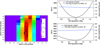 |
Fig. B.1 Study of Chi2 when fitting the EPiCA time series with a three-planet model. Left: Iso-contours of Chi2 as a function of planets c and d time lag. For each pair of planet c and d time lag with BJDref, a best fit of the time lag of planet b is computed, as well as the overall Chi2 on the 1151 points. The minimum Chi2 is at 3014, the average Chi2 per point is 2.6 (ms−1)2. Top right: Horizontal cross section of left image, with the variation of the time lag of planet b, and Chi2, as a function of the time lag of planet c, when the time lag of planet d is fixed to its overall best-fit value. Bottom right: Same as top, but the roles of planet d and c are inverted. For both panels, the variation of the time lag of planet b is very small, showing an absence of coupling between the phases (or time lags) of the three planets. |
New estimation of period for planet HD 40307 b
New estimation of period for planet HD 40307 c
New estimation of period for planet HD 40307d
References
- Artigau, É., Cadieux, C., Cook, N. J., et al. 2022, AJ, 164, 84 [NASA ADS] [CrossRef] [Google Scholar]
- Astudillo-Defru, N., Bonfils, X., Delfosse, X., et al. 2015, AAP, 575, A119 [NASA ADS] [CrossRef] [EDP Sciences] [Google Scholar]
- Baranne, A., Queloz, D., Mayor, M., et al. 1996, AAP, 119, 373 [NASA ADS] [Google Scholar]
- Bedell, M., Hogg, D. W., Foreman-Mackey, D., Montet, B. T., & Luger, R. 2019, AJ, 158, 164 [Google Scholar]
- Boisse, I., Eggenberger, A., Santos, N. C., et al. 2010, A&A, 523, A88 [NASA ADS] [CrossRef] [EDP Sciences] [Google Scholar]
- Bouchy, F., Pepe, F., & Queloz, D. 2001, A&A, 374, 733 [NASA ADS] [CrossRef] [EDP Sciences] [Google Scholar]
- Bouchy, F., Doyon, R., Artigau, É., et al. 2017, The Messenger, 169, 21 [NASA ADS] [Google Scholar]
- Cegla, H. M., Watson, C. A., Shelyag, S., Mathioudakis, M., & Moutari, S. 2019, ApJ, 879, 55 [NASA ADS] [CrossRef] [Google Scholar]
- Coffinet, A., Lovis, C., Dumusque, X., & Pepe, F. 2019, A&A, 629, A27 [NASA ADS] [CrossRef] [EDP Sciences] [Google Scholar]
- Collier Cameron, A., Ford, E. B., Shahaf, S., et al. 2021, MNRAS, 505, 1699 [NASA ADS] [CrossRef] [Google Scholar]
- Connes, P. 1985, Astrophys. Space Sci., 110, 211 [NASA ADS] [CrossRef] [Google Scholar]
- Cook, N. J., Artigau, É., Doyon, R., et al. 2022, PASP, 134, 114509 [NASA ADS] [CrossRef] [Google Scholar]
- Cosentino, R., Lovis, C., Pepe, F., et al. 2012, SPIE Conf. Ser., 8446, 84461V [Google Scholar]
- Cretignier, M., Dumusque, X., Allart, R., Pepe, F., & Lovis, C. 2020, AAP, 633, A76 [NASA ADS] [CrossRef] [EDP Sciences] [Google Scholar]
- Cretignier, M., Dumusque, X., Hara, N. C., & Pepe, F. 2021, AAP, 653, A43 [NASA ADS] [CrossRef] [EDP Sciences] [Google Scholar]
- Díaz, R. F., Ségransan,D., Udry, S., et al. 2016, A&A, 585, A134 [NASA ADS] [CrossRef] [EDP Sciences] [Google Scholar]
- Donati, J. F., Kouach, D., Moutou, C., et al. 2020, MNRAS, 498, 5684 [Google Scholar]
- Dravins, D., Lindegren, L., & Nordlund, A. 1981, AAP, 96, 345 [NASA ADS] [Google Scholar]
- Dumusque, X. 2018, AAP, 620, A47 [NASA ADS] [CrossRef] [EDP Sciences] [Google Scholar]
- Figueira, P., Lo Curto, G., & Mehner, A. 2021, Very Large TelescopeParanal Science Operations ESPRESSO User Manual, VLT-MAN-ESO-319963-666 [Google Scholar]
- González Hernández, J. I., Rebolo, R., Pasquini, L., et al. 2020, A&A, 643, A146 [EDP Sciences] [Google Scholar]
- Ivanova, A., Lallement, R., & Bertaux, J. L. 2023, AAP, 673, A56 [NASA ADS] [CrossRef] [EDP Sciences] [Google Scholar]
- Lafarga, M., Ribas, I., Lovis, C., et al. 2020, A&A, 636, A36 [NASA ADS] [CrossRef] [EDP Sciences] [Google Scholar]
- Mayor, M., & Queloz, D. 1995, Nature, 378, 355 [Google Scholar]
- Mayor, M., Udry, S., Lovis, C., et al. 2009, A&A, 493, 639 [NASA ADS] [CrossRef] [EDP Sciences] [Google Scholar]
- Meunier, N. 2021, arXiv e-prints [arXiv:2104.06072] [Google Scholar]
- Meunier, N., & Lagrange, A. M. 2020, AAP, 642, A157 [NASA ADS] [CrossRef] [EDP Sciences] [Google Scholar]
- Meunier, N., Lagrange, A. M., & Desort, M. 2010, AAP, 519, A66 [NASA ADS] [CrossRef] [EDP Sciences] [Google Scholar]
- Meunier, N., Lagrange, A. M., Borgniet, S., & Rieutord, M. 2015, AAP, 583, A118 [NASA ADS] [CrossRef] [EDP Sciences] [Google Scholar]
- Meunier, N., Pous, R., Sulis, S., Mary, D., & Lagrange, A. M. 2023, AAP, 676, A82 [NASA ADS] [CrossRef] [EDP Sciences] [Google Scholar]
- Nesvorný, D., & Morbidelli, A. 2008, APJ, 688, 636 [CrossRef] [Google Scholar]
- Pepe, F., Mayor, M., Delabre, B., et al. 2000, SPIE Conf. Ser., 4008, 582 [NASA ADS] [Google Scholar]
- Pepe, F., Mayor, M., Galland, F., et al. 2002, A&A, 388, 632 [NASA ADS] [CrossRef] [EDP Sciences] [Google Scholar]
- Pepe, F., Cristiani, S., Rebolo, R., et al. 2021, A&A, 645, A96 [NASA ADS] [CrossRef] [EDP Sciences] [Google Scholar]
- Queloz, D., Henry, G. W., Sivan, J. P., et al. 2001, AAP, 379, 279 [NASA ADS] [CrossRef] [EDP Sciences] [Google Scholar]
- Simola, U., Dumusque, X., & Cisewski-Kehe, J. 2019, AAP, 622, A131 [NASA ADS] [CrossRef] [EDP Sciences] [Google Scholar]
- Sulis, S., Lendl, M., Cegla, H. M., et al. 2023, AAP, 670, A24 [NASA ADS] [CrossRef] [EDP Sciences] [Google Scholar]
- Tuomi, M., Anglada-Escudé, G., Gerlach, E., et al. 2013, A&A, 549, A48 [NASA ADS] [CrossRef] [EDP Sciences] [Google Scholar]
- Wolszczan, A., & Frail, D. A. 1992, Nature, 355, 145 [CrossRef] [Google Scholar]
- Wright, J. T., & Eastman, J. D. 2014, PASP, 126, 838 [Google Scholar]
- Zechmeister, M., Reiners, A., Amado, P. J., et al. 2018, AAP, 609, A12 [NASA ADS] [CrossRef] [EDP Sciences] [Google Scholar]
EPiCA website https://github.com/aeictf/EPiCA
All Tables
Characteristics of three planets in the HD 40307 system from the HARPS 2008 campaign (Coffinet et al. 2019).
Characteristics of three planets in the HD 40307 system from the HARPS 2009 campaign.
All Figures
|
Fig. 1 Principle of shift-finding algorithm of Pierre Connes. Example of a spectral line at three epochs. Epoch 0 – reference (black), Epoch 1 – shifted by +2 km s−1 (red), Epoch 2 – shifted by +15 km s−1 (blue). The intensity change is measured within the dλ slice. This figure is similar to Fig. 4 in Connes (1985). |
| In the text | |
|
Fig. 2 Illustration of the simulation used to validate the Connes shift-finding algorithm and the error estimate. Black: CCF of original data (CCF1, right scale); green: CCF of simulated exposure shifted from original data (CCF2, left scale); red: weight function (left scale). |
| In the text | |
|
Fig. 3 Two RV time-series and their difference. Top: comparison between the RVs derived from the Gaussian fit and the EPiCA method. The data (RV changes in m s−1) are plotted as a function of exposure number. The pipeline RVs are plotted with their error bars, in a different color for each night. They were derived by subtracting from all pipeline RV data contained in each spectrum fits file the value of the first exposure: 31.3668 km s−1. Red points are obtained by the EPiCA method applied to the CCFs of the current exposure and the first exposure of night 24 (exposure n°10 when all nights are concatenated), taken as a reference. A constant 2 m s−1 was subtracted for clarity. Bottom: differences between the two time series of RV changes: Gaussian fit – EPiCA (CF1 applied to CCFtot). This difference shows an abrupt decrease (~1.3 ms−1) after exposure no. 615, corresponding to the transition from night 25 to night 26, which remains after that. |
| In the text | |
|
Fig. 4 Comparison of pipeline RV time series with three-planets modeling. The black dots represent the time series of changes of RV values contained in the official pipeline, obtained by subtracting the RV value of the first exposure of the first night. The thick pale gray solid line is the extrapolation of the sum of the three sine waves as determined from 2008 HARPS data. It does not closely fit the data because the extrapolation over 9 yr is sensitive to small errors in the periods. The dashed gray lines is the same as the solid gray line, but with planet b period shorter by 0.0004 day, corresponding to twice the claimed error bar for the period of planet b. The solid black line is the best fit to the pipeline RV data by adjusting the phases of the three planets. |
| In the text | |
|
Fig. 5 Same as Fig. 4, but with individual contributions of the planets. The three-planet best-fit curve is in black (solid line), while the dashed lines are each of the three sine waves representing the three planets: b (red), c (green), d (violet). The best-fit curve is the sum of the three planets plus a constant w0 = 1.5576 ± 0.515 m s−1. |
| In the text | |
|
Fig. 6 Histograms of RVs from the two different time series. They are obtained for the 406 exposures of night Dec24, after removal of linear fits to each series. The histogram is in red for the Gaussian fit and in black for EPiCA. Gaussian widths of histograms are indicated for each method. The EPiCA histogram is narrower than the Gaussian fit histogram. |
| In the text | |
|
Fig. 7 Same as Fig. 5, but for the time series obtained with EPiCA (red dots). The first exposure was taken as the reference. The best-fit curve is in red (solid line), while the dashed lines are each of the three sine waves representing the three planets: b (black), c (green), d (violet). The best-fit curve is the sum of the three planets plus a constant w0= −2.2106 ± 0.726 m s−1. |
| In the text | |
|
Fig. 8 Comparison of the best-fit models to the two time series. Solid lines are for the ESPRESSO pipeline. Dashed lines are for the EPiCA method. The red curve is for the total of three planets (+ the offset w0), while planets b, c, d have different colors. |
| In the text | |
|
Fig. 9 Residuals after subtraction of the best-fit model from the δRV official Gaussian fit (black points). It seems by eye that the average of groups of points do not always lie on the zero line. There is a bias that depends on the day of observation (numbers represent the night of December 2018 when HD 40307 was observed.) |
| In the text | |
|
Fig. 10 Residuals after subtraction of the best-fit model from the CF1 to CCFtot time series (red points). It seems by eye better aligned on the Zero line (solid black line) than for the δRV time series of Fig. 9. |
| In the text | |
|
Fig. 11 Mean residual for each night as a function of time (BJD-BJDref). Black: Gaussian fit. Red: EPiCA method (CF1 on CCFtot). The error bars are computed as the standard deviation divided by sqrt(number of exposures). The two points for night 25 (around 3.2 days) are not independent. |
| In the text | |
|
Fig. 12 Model-data comparison using CCF ratios. Top: expected ratio of two CCFs with unchanged shape and various Doppler shifts (colored lines), and ratios using the four periods of night 24 (black lines). The same curve is observed for ratios of parts 2, 3, and 4 to part 1. It does not resemble the expected variation for a simple shift and indicates a change in shape during the first and second parts of the night. Bottom: ratios of pairs formed by the first two consecutive stacked CCFtot obtained during the same night, for nights 24 to 28 (numbers indicated on the plot for 26 to 28). One CCFtot is drawn (gray line). There is a systematic bump centered on the CCFtot, indicative of an increase in signal near the center during the first and second parts of each daily pair. The increase is larger for the latest nights. The ratio for the two last parts of night 24 is shown for comparison (pink line). There is no increase in this case, a sign of absence of shape variation during this period. |
| In the text | |
|
Fig. 13 EPiCA profiles DRV(i) along the velocity grid for pairs of time periods (lines with markers). Offsets of 30 m s−1 are applied between two consecutive profiles, except for the two top curves, which are plotted together. The actual zero value is indicated by a black thin line. The size of the markers is increasing with the individual weight for each series. A typical weight function is also plotted (thin dot-dashed line). The two most central values suffer from additional uncertainties due to the limited velocity sampling and are delimited by a rectangle. (Top curves) For pairs made of the second to fourth parts of night 24, the profiles are flat within the error bars, showing no significant change in shape; this is consistent with the constancy observed using ratios, pointing to a stabilization of the instrument. For each of the other pairs (lower curves) containing the first and second parts of a night, one can observe departures from a flat profile, and a similar shape with an amplitude increasing from night 24 to night 28. This typical shape of DRV(i) is induced by a decrease in contrast (see text), consistent with the same type of behavior as the bump measured using CCF ratios (Fig. 12). It could be due to a stellar process or to an artifact. |
| In the text | |
|
Fig. 14 Ratios of pairs of CCFtot taken one day apart along the HD 40307 campaign. They are plotted as a function of RV(i), the abscissae of the CCF. There are two pairs for each couple of consecutive nights. The ratios are vertically displaced by multiples of 0.005 for each pair for clarity. The first and second pair of the night are respectively in red and in black. The standard deviation of the curve is indicated. The upper curves are two ratios of night 24, whose wiggles are small and likely representative of the noise level for all curves. There is a marked departure from flatness for the ratio 26/25, as expected from the Kepler fit RV drop between nights 25 and 26. However, the observed ratio is very different from a model ratio in the case of a pure Doppler shift, as can be seen from the comparison with the superimposed model for a pure shift of –5 m s−1 (gray curve). Therefore, this set of curves indicates directly a change in shape between the two nights. |
| In the text | |
|
Fig. 15 Same as Fig. 13, for four pairs of stacks that are one day apart over the five nights from night 24 to 28. Each pair consists of using either the first or the second parts of night. Offsets of 40 m s−1 are applied between two pairs of these EPiCA profiles. The actual zero value is indicated by a black thin line. The DRV curve for the pair 25–26 shows a different pattern in comparison with the other pairs, with a strong difference between the blue side and the red side. |
| In the text | |
|
Fig. B.1 Study of Chi2 when fitting the EPiCA time series with a three-planet model. Left: Iso-contours of Chi2 as a function of planets c and d time lag. For each pair of planet c and d time lag with BJDref, a best fit of the time lag of planet b is computed, as well as the overall Chi2 on the 1151 points. The minimum Chi2 is at 3014, the average Chi2 per point is 2.6 (ms−1)2. Top right: Horizontal cross section of left image, with the variation of the time lag of planet b, and Chi2, as a function of the time lag of planet c, when the time lag of planet d is fixed to its overall best-fit value. Bottom right: Same as top, but the roles of planet d and c are inverted. For both panels, the variation of the time lag of planet b is very small, showing an absence of coupling between the phases (or time lags) of the three planets. |
| In the text | |
Current usage metrics show cumulative count of Article Views (full-text article views including HTML views, PDF and ePub downloads, according to the available data) and Abstracts Views on Vision4Press platform.
Data correspond to usage on the plateform after 2015. The current usage metrics is available 48-96 hours after online publication and is updated daily on week days.
Initial download of the metrics may take a while.