| Issue |
A&A
Volume 663, July 2022
|
|
|---|---|---|
| Article Number | A143 | |
| Number of page(s) | 17 | |
| Section | Planets and planetary systems | |
| DOI | https://doi.org/10.1051/0004-6361/202142262 | |
| Published online | 26 July 2022 | |
A novel framework for semi-Bayesian radial velocities through template matching
1
Instituto de Astrofísica e Ciencias do Espaço, Universidade do Porto,
CAUP, Rua das Estrelas,
4150–762
Porto, Portugal
e-mail: amiguel@astro.up.pt
2
Departamento de Física e Astronomia, Faculdade de Ciencias, Universidade do Porto,
Rua do Campo Alegre,
4169–007
Porto, Portugal
3
Instituto de Astrofísica de Canarias (IAC),
38205
La Laguna,
Tenerife, Spain
4
Universidad de La Laguna (ULL), Departamento de Astrofísica,
38206
La Laguna,
Tenerife, Spain
5
Département d'astronomie de l'Université de Genève,
Chemin Pegasi 51,
1290
Versoix, Switzerland
6
European Southern Observatory,
Alonso de Córdova 3107, Vitacura,
Región Metropolitana, Chile
7
INAF - Osservatorio Astrofisico di Torino,
via Osservatorio 20,
10025
Pino Torinese, Italy
8
Centro de Astrobiología (CSIC-INTA),
Crta. Ajalvir km 4,
28850
Torrejón de Ardoz, Madrid, Spain
9
INAF - Osservatorio Astronomico di Trieste,
via G. B. Tiepolo 11,
34143
Trieste, Italy
10
Consejo Superior de Investigaciones Cientícas,
Spain
11
Instituto de Astrofísica e Ciencias do Espaço, Faculdade de Ciencias da Universidade de Lisboa,
Campo Grande,
PT1749–016
Lisboa, Portugal
12
Faculdade de Ciências da Universidade de Lisboa (Departamento de Física),
Edifício C8,
1749–016
Lisboa, Portugal
13
Centro de Astrofísica da Universidade do Porto,
Rua das Estrelas,
4150–762
Porto, Portugal
14
Department of Physics, and Institute for Research on Exoplanets, Université de Montréal,
Montréal,
H3T 1J4
Canada
15
Centro de Astrobiología (CAB, CSIC-INTA),
Depto. de Astrofísica, ESAC campus,
28692
Villanueva de la Cañada (Madrid), Spain
Received:
20
September
2021
Accepted:
25
April
2022
Context. The ability to detect and characterise an increasing variety of exoplanets has been made possible by the continuous development of stable, high-resolution spectrographs and the Doppler radial velocity (RV) method. The cross-correlation function (CCF) method is one of the traditional approaches used to derive RVs. More recently, template matching has been introduced as an advantageous alternative for M-dwarf stars.
Aims. We describe a new implementation of the template matching technique for stellar RV estimation within a semi-Bayesian framework, providing a more statistically principled characterisation of the RV measurements and associated uncertainties. This methodology, named the Semi-Bayesian Approach for RVs with Template matching, S-BART, can currently be applied to HARPS and ESPRESSO data. We first validate its performance with respect to other template matching pipelines using HARPS data. We then apply S-BART to ESPRESSO observations, comparing the scatter and uncertainty of the derived RV time series with those obtained using the CCF method. We leave a full analysis of the planetary and activity signals present in the considered datasets for future work.
Methods. In the context of a semi-Bayesian framework, a common RV shift is assumed to describe the difference between each spectral order of a given stellar spectrum and a template built from the available observations. Posterior probability distributions are obtained for the relative RV associated with each spectrum using the Laplace approximation, after marginalization with respect to the continuum. We also implemented, for validation purposes, a traditional template matching approach, where a RV shift is estimated individually for each spectral order and the final RV estimate is calculated as a weighted average of the RVs of the individual orders.
Results. The application of our template-based methods to HARPS archival observations of Barnard’s star allowed us to validate our implementation against other template matching methods. Although we find similar results, the standard deviation of the RVs derived with S-BART is smaller than that obtained with the HARPS-TERRA and SERVAL pipelines. We believe this is due to differences in the construction of the stellar template and the handling of telluric features. After validating S-BART, we applied it to 33 ESPRESSO GTO targets, evaluating its performance and comparing it to the CCF method as implemented in ESO’s official pipeline. We find a decrease in the median RV scatter of ~10 and ~4% for M- and K-type stars, respectively. Our semi-Bayesian framework yields more precise RV estimates than the CCF method, in particular in the case of M-type stars where S-BART achieves a median uncertainty of ~15 cm s−1 over 309 observations of 16 targets. Further, with the same data we estimated the nightly zero point (NZP) of the instrument, finding a weighted NZP scatter of below ~0.7 m s−1. Given that this includes stellar variability, photon noise, and potential planetary signals, it should be taken as an upper limit on the RV precision attainable with ESPRESSO data.
Key words: techniques: radial velocities / techniques: spectroscopic / planets and satellites: detection / methods: data analysis / planets and satellites: terrestrial planets / methods: statistical
© A. M. Silva et al. 2022
 Open Access article, published by EDP Sciences, under the terms of the Creative Commons Attribution License (https://creativecommons.org/licenses/by/4.0), which permits unrestricted use, distribution, and reproduction in any medium, provided the original work is properly cited.
This article is published in open access under the Subscribe-to-Open model. Subscribe to A&A to support open access publication.
1 Introduction
Finding and characterising other Earths – rocky planets with the physical conditions needed to hold liquid water on their surface – is one of the boldest goals of present-day astrophysics. The discovery (e.g. Mayor et al. 2011, 2014; Hsu et al. 2019; Rosenthal et al. 2021) that rocky planets are very common around solartype stars, that is, late F, G, and early K stars, made this goal more achievable and motivated the development of a new generation of ground- and space-based instruments and missions (e.g. ESPRESSO; Pepe et al. 2021; PLATO, Rauer et al. 2014, HIRES@ELT; Marconi et al. 2021).
One of the most prolific exoplanet discovery methods is the radial velocity (RV) method, which is based on the detection of variations in the velocity of a star along our line of sight induced by the gravitational pull of planetary companions. However, the identification of Earth-like planets orbiting solar-type stars poses a significant challenge: Earth itself induces a signal with an amplitude of only ~9 cm s−1 on the Sun. In order to achieve this RV precision domain, a new generation of spectrographs have been developed. An example of such a state-of-the-art spectrograph is the Échelle SPectrograph for Rocky Exoplanets and Stable Spectroscopic Observations (ESPRESSO), which was built to reach a precision of 10 cm s−1 with a wavelength coverage from 380 to 788 nm (Pepe et al. 2021).
The first confirmed detection of an exoplanet around a solar-type star, 51 Pegasi b (Mayor & Queloz 1995), was achieved with radial velocities computed using the cross correlation function (CCF) method. In the early stages of development of this method, a binary mask with fixed non-zero weights attributed to the expected positions of stellar absorption lines was cross-correlated with the spectra (Baranne et al. 1996). However, as deep sharp lines contain more information than broad and shallower ones (as shown by the methodology introduced in Bouchy et al. 2001) the masks were improved by associating different weights to different lines (Pepe et al. 2002), depending on the RV information present in them, such that deep lines contribute more to the final CCF profile than shallow ones.
Although the CCF method has been widely used, building the masks can be a challenging task in some situations, especially for M dwarfs (e.g. Rainer et al. 2020; Lafarga et al. 2020). The high number of stellar spectral lines, due to the lower temperatures of M-type stars, results in the presence of a larger number of spectral lines, with most of them being spectro-scopically blended, which makes the construction of the CCF mask and the fitting of the CCF profile more difficult. For such cases, it has been shown that template matching can surpass the CCF method (e.g. Anglada-Escudé & Butler 2012; Zechmeister et al. 2018; Lafarga et al. 2020), as the stellar template will contain a large majority of the lines in the stellar spectrum. This is a data-driven method, where each spectrum is compared with a template built from available observations, and has been implemented in HARPS-TERRA (Anglada-Escudé & Butler 2012), NAIRA (Astudillo-Defru 2015), and SERVAL (Zechmeister et al. 2018). More recently, new approaches to RV estimation have emerged based on line-by-line measurement of RV shifts (Dumusque 2018; Cretignier et al. 2020), modelling of the observed spectrum as a linear combination of a time-invariant stellar spectrum and a time-variant telluric spectrum (wobble; Bedell et al. 2019), or pairwise spectrum comparison through Gaussian process interpolation (GRACE; Rajpaul et al. 2020).
In the following sections, we recast the template matching approach within a semi-Bayesian framework, and then evaluate the performance of template-based RV-extraction methodologies when applied to ESPRESSO data. In particular, in Sect. 2 we discuss how the spectral data are processed, the stellar template is created, and the telluric features are removed. In Sect. 3 we revisit the classical template matching algorithm, and in Sect. 4 we discuss the working principles of our semi-Bayesian template matching approach, as well as our strategy to efficiently characterise the posterior distribution of the model. In Sect. 5 we evaluate the performance of our template matching algorithm using data from (i) 22 HARPS observations of Barnard’s star, to validate our template-based methodologies by comparison with the results of other template matching pipelines applied to a common set of spectra; and (ii) 1046 ESPRESSO observations of 33 M-, K-, and G-type stars, which are the main focus of this paper. To the ESPRESSO dataset we apply the classical template matching approach, the CCF of the official ESO pipeline, and our semi-Bayesian approach, allowing the comparison of RV scatter and uncertainties, and the estimation of an upper bound for RV precision. We refrain from studying the impact that stellar activity has on S-BART-derived RVs, as our ESPRESSO sample mainly contains quiet stars. Such an endeavour would translate into a large-scale modelling effort, which lies outside the scope of the current paper. Lastly, in Sect. 6 we discuss some limitations of the developed methodology and present some possible improvements.
2 Model Preparation
In this section, we discuss the stages of data processing - common to all instruments supported by our algorithm – that must must be applied before estimating RVs from spectra. We also discuss the creation of the stellar template and removal of telluric features through the use of synthetic spectra of Earth’s atmosphere. Figure 1 shows the order in which the different procedures are applied.
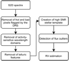 |
Fig. 1 Workflow of the processing stage that we apply before the RV estimation. |
Central wavelength (measured in air) and size of the spectral regions removed from the spectra.
2.1 Pre-Processing Data
The extraction of the spectral orders from the image and the necessary calibrations and corrections are handled by the official data reduction software (DRS) used with the respective instruments. Regions around spectral lines that are typically used as activity indicators or are clearly identifiable as emission features are removed from the spectra.
In Table 1, we identify the central wavelengths and the size of the spectral region that is removed around each feature. The chosen windows have been verified with the spectra of M-type stars. We also remove bad or hot pixels that are flagged by the official pipeline of the instrument, as well as those that have null data. When considering the mentioned effects, if we remove more than 75% of an order in a stellar spectrum we do not consider the order when estimating RVs.
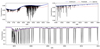 |
Fig. 2 Comparison between the telluric spectrum obtained from Tapas (black), with the continuum level obtained with a median filter (dashed blue line), and the telluric threshold (dotted red line) built from the continuum, for three spectral regions. |
2.2 Telluric Template
Earth’s atmosphere absorbs radiation, imprinting telluric absorption features in spectra acquired with ground-based spectrographs. The impact of this phenomenon strongly depends on the wavelength range and resolution of the spectrograph, the airmass of the observations, water vapour content, and weather conditions (e.g. Figueira et al. 2012; Cunha et al. 2014), and if not corrected, it can lead to biased and less precise RV estimates. Even shallow telluric lines, or micro-telluric lines, can induce a significant bias of about 10–20 cm s−1 (Cunha et al. 2014), which is approximately equal to or larger than the signal produced by an Earth-like world around a solar-type star.
The identification and removal of telluric features from stellar spectra is therefore essential for the estimation of accurate and precise RVs. For this purpose, we use a synthetic spectrum of the transmittance from Earth, with a resolution equal to that from the instrument mode obtained through the Tapas (Bertaux et al. 2014) web interface1. We start by estimating the continuum level of the transmittance spectrum through a rolling median filter that spans over 1000 points (though near the edges we reduce the window to 50 points to minimise numerical artifacts due to the choice of the filter’s boundary conditions). We flag domains where the transmission is lower than a given threshold – by default this represents 99% of the continuum level – as wavelength domains affected by tellurics. Figure 2 shows the behaviour of the rolling median filter. In regions with shallower telluric features, the continuum estimation is not affected. However, that is no longer the case in regions where there is a greater presence of deeper features (bottom panel). Despite this, the chosen threshold is still enough to properly identify the telluric features, as seen in the bottom panel of the figure. It is important to note that this choice of threshold is not able to detect shallower telluric features, as seen in the upper panels of the figure. However, a more restrictive threshold would result in a rejection of larger spectral regions across the wavelength coverage of the instrument. Therefore, we attempt to maximise the spectral coverage whilst still removing the deeper telluric features.
We must also take into account the RV component introduced by the motion of Earth around the barycenter of the Solar System (and as such nicknamed the Barycentric Earth RV, or BERV). This motion introduces a Doppler shift in the observed spectrum that can be corrected by shifting the reference frame from Earth to an inertial one, the barycenter of the Solar System. This correction is incorporated, usually by default, in the official pipeline of the spectrograph, as is the case for ESPRESSO, where the wavelength solution is shifted by the corresponding value. As the telluric line wavelengths are fixed on the detector on the reference frame of Earth, their position relative to the stellar lines will change, and in the BERV-corrected spectra the telluric lines will appear as shifted by -BERV. To take into account this relative movement, we discard a wavelength domain around each feature corresponding to the maximum BERV (~30 km s−1, obtained for stars along the direction of Earth’s orbit).
2.3 Stellar Template
The stellar template is the most important component of our model, as it is assumed to be a high signal-to-noise-ratio (S/N) model spectrum that very accurately represents the stellar spectrum, which is assumed to be immutable. Any observed spectrum is assumed to differ from this template only as a result of a Doppler-shift induced by the stellar RV. This high-S/N template is built by combining the information of multiple observations of the same star.
2.3.1 Building the Template
The stellar template is built on an order-by-order basis, so that it can accurately represent the stellar spectra. Its construction starts with the choice of the reference frame for the template, that is, the wavelength solution henceforth associated with it. For this purpose, we use the BERV-corrected observation with the smallest uncertainty in the RV estimated by the ESO pipeline (through the CCF method).
We decided to place our stellar template in a rest frame, that is, at a RV of zero. To do so, we remove the contribution of the stellar RV from the wavelengths of the template; this contribution is either estimated beforehand through the CCF approach or a previous iteration of our template matching procedure. The next step is to remove, from all observations, the contribution of their own stellar RVs. As the wavelengths of the spectra will not be an exact match to those from the template, we have to interpolate them to a common wavelength grid, namely the one from the template. For this purpose, we apply a cubic splines algorithm (see Sect. 3.3 of Press 1992). Due to the BERV, the stellar spectrum will shift on the CCD, and thus different spectra will have different starting and ending wavelengths in each spectral order (see Fig. 3). For each order, we select the wavelengths common to all spectra in order to avoid different S/Ns within the same order of the template. Finally, we compute the mean of the fluxes in order to build a high-S/N stellar template. We calculate the mean in order to keep the count level at a physically meaningful value and avoid possible numerical issues further on in the process.
Lastly, we must also consider the presence of telluric features in the data. Even though the wavelength domains affected by the deeper features can be removed with the methodology discussed in Sect. 2.2, micro-tellurics will not be identified by our mask and will consequently still be present in the individual observations. As seen in Cunha et al. (2014), micro-tellurics can have a considerable impact on the accuracy and precision of the estimated RVs, in particular when obtained from data acquired with instruments as stable as ESPRESSO. By constructing the template from a large number of spectra obtained at different periods of the year, that is, by having a wide BERV range, their effects on the spectral template can, in principle, be minimised by averaging them out. However, as this condition is not always met, we mitigate their impact by using only observations whose associated airmass is smaller than 1.52 in the building of the spectral template, as the depth of the telluric features increases with airmass (Figueira et al. 2010). This choice allows us to strike a balance between (i) the number of observations that are discarded due to high micro-telluric contaminations and (ii) the number of observations that can be used in the construction of the template. Furthermore, at higher airmasses, the correction of the atmospheric dispersion is not as efficient as it is for lower airmasses (Wehbe et al. 2019). Thus, this selection is an attempt to select a set of homogeneous spectra to be used in the construction of the stellar template.
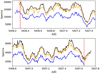 |
Fig. 3 BERV-corrected spectra of different observations at the start (top) and end (bottom) of a spectral order. Top panel: dashed red line represents the minimum wavelength, so that all (of the presented) orders have data at the start of the order. Bottom panel: dashed red line represents the last wavelength at which all orders have data. |
2.3.2 Estimation of Uncertainty in the Stellar Template
The stellar template will be affected by some uncertainty given that it is built as a mean of N spectra, all affected by flux measurement uncertainties. Within this subsection, we start by discussing the calculation of the uncertainties associated with the stellar template, and then compare these with the uncertainties in both low- and high-S/N observations. Lastly, we touch upon the computational trade-offs that must be made to ensure performance of the algorithm.
If each spectrum had the same S/N, then we would expect the S/N of the template to be approximately equal to  multiplied by the S/N of each observation. Under this assumption, we would need 100 observations to achieve a mean uncertainty (standard deviation) per flux of one order of magnitude smaller than that associated with any single observation. As many targets will have fewer observations, we decided to propagate the uncertainties associated with the template towards the final RV estimate, as discussed in Sects. 3 and 4. For this purpose, we have to take into account that both the spectral data and the template are interpolated with cubic splines in two different stages: during the creation of the stellar template and in the RV-extraction procedure. In Appendix A we describe the analytical uncertainty propagation through the cubic spline interpolation algorithm.
We studied the characteristics of the uncertainty in the template by selecting the available observations of an M4 star (Nspectra = 21) from the sample used in Sect. 5.2.3, which allows us to assess the need to account for them during the RV estimation. The chosen observations were made after ESPRESSO’S fiber link upgrade in June 2019 (Pepe et al. 2021) and we selected data from the 100th spectral order (central wavelength of 541 nm). In order to evaluate the impact of the number of spectra used to construct the template, we selected two sets of observations: those with an airmass below 1.2 (N = 8); and those with an airmass below 1.5 (N = 13). After creating the stellar templates, we align them with each observation and interpolate the flux of the template to the wavelength solution of the observation, also propagating the uncertainties in the template. We then compare these templates against those associated with the spectra, as computed by the ESO pipeline. A direct comparison is not possible, as observations with lower flux values also have lower photon noise and, consequently, smaller flux uncertainties. Instead, we compute the S/Ns of the template and spectra for each pixel of the order.
Figure 4 shows that an increase in the number of observations used to construct the template leads to an increase in its S/N compared to the individual observations, as one would expect. The comparison for the lower S/N spectra (non-filled bins) reveals that the two stellar templates have uncertainties that are close to one order of magnitude smaller than those found for the observations. Unfortunately, that is not the case for the higher S/N observations, namely those with an S/N in the 100th order of at least 100. For a more detailed analysis, Table 2 shows the comparison of each template against three different sets of observations: with all observations; with only the observations used in the construction of the template; and with observations whose S/N is at least 100. We find that in all cases, the median S/N is larger than  , a difference explained by the fact that the selected observations all have different S/Ns. From this analysis, we see that the S/N of the template is not one order of magnitude larger than that of the observations, confirming the need to account for those uncertainties.
The main problem with our uncertainty propagation procedure, which is described in Appendix A, lies in its computational efficiency, as it requires the inversion of large matrices. Whilst it is feasible to use this procedure for the calculation of uncertainties during the creation of the stellar template, it is a computational bottleneck in the interpolation of the stellar template for each tentative RV shift that is tested during the RV-extraction procedure. In an attempt to mitigate this problem, we decided to evaluate whether or not we could estimate the template flux uncertainties by interpolation instead of applying the analytical uncertainty propagation procedure.
This approximation was tested by interpolation of the two templates previously used in Fig. 4 and a subsequent comparison of the flux uncertainties obtained through both methods. We find, for the two templates, that the interpolation of flux uncertainties (standard deviations) results in their overestimation by a factor of 1.07 ± 0.05 across the 21 observations. Even though there is a slight increase in the template uncertainty, we do not deem it to be problematic, especially when also considering the high S/N of the template itself, when compared with the individual observations. With this in mind, during the RV extraction, we propagate the uncertainties in the stellar template by interpolating them to the desired wavelength solution.
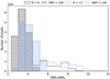 |
Fig. 4 Histogram of the S/N, for the 100th order, of the template and each of the 21 individual observations of an M4 star, obtained after the fiber link upgrade of ESPRESSO in mid-2019. In order to compare the impact of the number of observations used to construct the template on its associated uncertainty, one template was built with 8 observations (black curve) and the other with 13 observations (blue curve), selected by the airmass at the start of each observation. For all observations we also highlight the comparison with observations with a S/N of at least 100 for the selected spectral order by filling the bins with the corresponding colour. |
Analysis of the S/N between each of the two templates and three different subsets of the available observations.
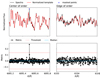 |
Fig. 5 Outlier removal routine for two regions of the same order, with respect to an observation for which outlier identification achieved convergence after the first iteration. For representation purposes, we normalized the flux in the center and the edge of the order. Top row: comparison between the stellar template (red line) and the spectra (black line). The blue crosses represent the points that were flagged by the method. Bottom row: differences between the template and spectra (black points). The blue line is the median value, whilst the dotted red lines represent a 6σ difference from it. |
2.3.3 Removal of Outliers in the Spectra
Even though the stellar template is generally a good match to the stellar spectrum associated with any given observation, there are some regions where such an assumption does not hold, such as in the top row of Fig. 5, highlighting the need to remove so-called flux outliers before starting the RV-estimation procedure. It is important to note that any point that was discarded in Sect. 2.1 will be ignored during the search for outliers.
We start by aligning the stellar template and a given spectrum using the initial guess for the associated RV, either estimated through the CCF method or a previous application of template matching. We then adjust both continuum levels by fitting a first-degree polynomial with slope m and intercept b to the ratio between the spectrum and template. Finally, we compute the logarithm of the ratio between spectrum and template and use it as a metric to flag mismatch regions:
 (1)
(1)
where  is the flux of the stellar spectrum,
  is the first-degree polynomial, and
  is the interpolated stellar template, all evaluated at wavelength λi. We use the logarithm instead of the ratio in order to mitigate the larger differences that exist for lower S/N regions closer to the edges of the spectral orders. This metric ensures performance for a large dynamic range of fluxes as seen inside a single order. Further, as the spectra are noisy and we are mostly interested in finding large flux differences, we allowed for a large tolerance in the identification of outliers. We consider all points whose metric is more than 6σ3 away from the median metric (of the entire order) to be outliers. Using lower thresholds would result in excessive flagging in both edges of the order, as the differences (in absolute values) between spectra and template are larger.
In Fig. 5 we can see an application of the algorithm to two spectral chunks. Starting in the left panel, we find minimal (relative) differences between the spectrum and the normalized template, with the exception of the clear outlier that is flagged by our routine. On the right panel, we see that the spectrum is noisier, resulting in a poorer match between spectrum and template. Nonetheless, our algorithm does not flag any point, as there are no clear outliers.
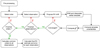 |
Fig. 6 Schematic of the classical template matching RV-estimation procedure, including the computation of the uncertainties in the stellar template. We iterate over orders at the highest level, and not observations, in order to optimise the computational efficiency of the method. |
3 Classical Template Matching
In order to benchmark our methodology to estimate radial velocities, we first implemented a template matching approach similar to those used to build the HARPS-TERRA (Anglada-Escudé & Butler 2012) and SERVAL (Zechmeister et al. 2018) pipelines. In Fig. 6 we provide a high-level schematic of the RV-estimation procedure, whose boxes are described with more detail within this section.
Radial velocities are determined individually for each order i through least squares minimisation:
![${\chi ^2} = \mathop \sum \limits_{i = 1}^{{N_{{\rm{pixels}}}}} {1 \over {\sigma _{\rm{S}}^2 + \sigma _{\rm{T}}^2}}*{\left[ {{S_{{\lambda _i}}} - p{{\left( {m,b} \right)}_{{\lambda _i}}}{T_{{\lambda _i}}}} \right]^2},$](/articles/aa/full_html/2022/07/aa42262-21/aa42262-21-eq8.png) (2)
(2)
where  is the flux of the stellar spectrum, σS is its associated (1σ) uncertainty,
  is the first-degree polynomial mentioned in Sect. 2.3.3,
  is the stellar template, and σT is its (1σ) uncertainty, all evaluated at wavelength λi
The χ2 minimisation is performed with scipy’s (Virtanen et al. 2020) implementation of the Brent method inside awindow with a default size of 200 m s−1 centered around the previous RV estimate. The stellar template is Doppler-shifted by each tentative RV and interpolated with a cubic spline algorithm to the wavelength solution of the spectra. Similarly to the creation of the stellar template described in Sect. 2.3.2, the uncertainties of the stellar template are also interpolated to the new wavelength solution. After the minimiser converges, we use the proposed RV value and two adjacent ones, separated by the RV interval ±∆RV, to numerically fit a parabola to the curve, similarly to Zechmeister et al. (2018). By default, we assume ∆RV to be 10 cms−1 for ESPRESSO and 50 cms−1 for HARPS. For further details with respect to this fit, we refer to Sect. 10.2 of Press (1992). The fitted parabola is then used to correct the RV estimate and calculate its uncertainty:
 (3)
(3)
where RVorder is the final RV estimate, σRVis the measurement (1σ) uncertainty, RVmin is the RV value that minimises Eq. (2), while m − 1 and m + 1 identify the two RV values selected at a distance ∆RV from RVmin.
If the minimiser proposes a value near the edges of the search window, there is no guarantee that the proposal is the true minimum of the χ2 curve. Thus, whenever the result of the Brent minimisation lies within 5∆RV of either edge of the search window, we define a new one centered at the edge of the interval, with a size of 30 m s−1 and re-start the minimisation procedure. As we do not expect such large differences between the CCF RVs and those obtained through a template matching method, we discard the entire order if, once again, we do not find a minimum RV that meets the aforementioned criteria within the new search window.
In Fig. 7 we show the comparison of the CCF-based ESPRESSO pipeline (DRS) RV estimate and that obtained through Eq. (3) for one spectral order. There is a very good match between the parabolic fit and the full χ2 curve. Furthermore, the advantages of using the Brent method for the minimisation are evident: it can quickly achieve convergence, greatly increasing the computational efficiency of the routine (e.g. in the case shown in Fig. 7 we only have to sample Eq. (2) four times before achieving convergence for the spectral order).
After estimating a RV with respect to each individual order, we combine them through a weighted mean with inverse variance weights (Schmelling 1995) in order to calculate the final RV estimate (υ) and uncertainty (σv) for the entire observation:
 (4)
(4)
where υi is the RV of order i and  is its associated (1σ) uncertainty, while N is the total number of orders for which we estimated an RV. The value of
  is estimated whilst ignoring any correlations that might exist between the assumed independent spectral orders.
As we see in this section and in Sect. 2.1, some spectral orders may be discarded for some of the observations. In this case, different wavelength domains would be used in the estimation of the final RVs of the different observations. This could introduce additional RV variability within the considered set of observations that is due to possible differences in the spectral information contents and systematic effects in each spectral order. In order to avoid this additional source of RV variability, we retain only the wavelength domain that is common (i.e. not discarded) to all observations. The drawback to this approach is that the inclusion of a single observation can cause the removal of a large number of orders. In this case, there would be a smaller loss of information if the entire observation was discarded instead. We currently have no way of evaluating this trade-off other than by performing a manual inspection of the number of orders removed per observation, and then determining how all the RV final estimates and their uncertainties change in the case where one or more observations are discarded from the full RV-estimation procedure.
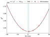 |
Fig. 7 The χ2 curve for the 100th spectral order of an ESPRESSO observation of GJ699 (black line), sampled with a step of 10 cm s−1 inside the 200 m s−1 search window centered on the ESPRESSO DRS estimate. The parabolic fit is shown as the red line. The red circles represent the RV estimates provided by the Brent method before meeting the convergence criteria. The dashed blue line is the final RV, calculated with Eq. (3), and the dotted green line the ESPRESSO DRS estimate for the given observation. |
4 Semi-Bayesian Template Matching
The current approaches to template matching assume that Doppler-shifts associated with the different spectral orders are independently generated. However, this is clearly not the case for the stellar RV component induced by orbiting bodies such as planets or companion stars. In fact, such shifts are achromatic, that is, they are independent of the wavelengths at which they are measured. Relative RV estimates, such as those obtained through template matching, are primarily used to detect orbiting bodies and characterise their masses and orbits. Thus, consistency then suggests that one should use a single RV shift to simultaneously describe the differences for all orders between a given spectrum and the stellar template. Any effects that may hinder the correct estimate of this single RV shift, such as those of instrumental origin or due to stellar activity, should be dealt with explicitly, either through modelling or exclusion of affected spectral data.
The casting of RV estimation through template matching into a Bayesian statistical framework allows consistent and straightforward characterisation of the RV (posterior) probability for any observation, including marginalisation with respect to the parameters of the first-degree polynomials that are used to adjust the continuum level of spectra and template. However, within a Bayesian framework, all aspects of the model considered need to be specified prior to the actual data analysis, that is, the information contained in the data cannot be used twice, once for building the model (prior specification) and also for comparison with its predictions (through the likelihood). Unfortunately, the latter takes place in the context of template matching, and the available spectra are used to specify the template (model building) as well as to estimate the RVs at the times of spectra acquisition (data analysis). This is the reason why we call semi-Bayesian to the template matching approach for RV estimation described schematically in Fig. 8 and with greater detail in this section.
This approach has been implemented in a pipeline capable of processing HARPS and ESPRESSO data, named S-BART4. It is important to note that the S-BART pipeline allows the use and configuration of all techniques that have been described in this manuscript, including the traditional template matching approach, that is, the one introduced in Sect. 3.
4.1 The RV Model
We apply our RV model independently to each observation. It contains only one parameter of interest, the relative RV with respect to some reference frame, which is the one for which the template RV is zero. Our aim is to characterise the RV posterior probability distribution given each observed spectrum, which is proportional to the product of the RV prior probability distribution multiplied by the likelihood of the spectral data. We assume an uninformative prior, taking the form of a uniform probability distribution. The likelihood of the full spectral data, conditioned on a given RV value, will be assumed to be equal to the product of the likelihoods of the fluxes measured for each pixel, that is, the flux measurements for all pixels are considered to be independent. In practice, we first calculate the likelihood of the spectral data for each order, and then multiply these to obtain the full likelihood.
However, our RV model also contains so-called nuisance parameters that we have to marginalise over. The nuisance parameters are those involved in the template matching procedure described in Sect. 2.3: the slope, m, and intercept, b, of the first degree polynomial that is used to adjust the continuum level of the template spectrum to that of each spectrum under analysis; and the flux associated with each pixel in the template, relative to the continuum. The latter are effectively latent variables – affected by some uncertainty – characterised in Sect. 2.3.2. Each spectral order has its own set of independent nuisance parameters, and therefore the marginalisation procedure can be applied order by order. We assume the joint prior distribution with respect to all model parameters to be separable, that is, able to be written as the product of prior distributions specifically associated with each parameter. Thus, in practice, the marginalisation procedure involves the integration of the product of the prior distributions with respect to the nuisance parameters multiplied by the likelihood as a function of all parameters.
The likelihood of a given observed spectrum, S, conditioned on an assumed RV value, is therefore given by
 (5)
(5)
where Norders is the total number of orders in the spectrum that are not discarded as a result of the procedure discussed in Sect. 3, Ni is the number of data points in order i (usually smaller than the number of pixels in the order because of the masking of spectral regions contaminated by telluric lines and outlier removal), and  and
and  are the fluxes associated with pixel λi,j in the (interpolated) template and spectrum, respectively. We assume that the prior probabilities, P(mi, bi) and
  , are uninformative Gaussians. Given that the last probability is also a Gaussian, with an expected value that is a linear function of λi,j, that is
  , in the limit of infinite variance for the prior probabilities, the integral is equal to a Gaussian and
 (6)
(6)
where Si is a vector with the flux measurements for all pixels in order i, A is equal to  , C is given by
  , and ni is the number of data points in order i (for more details see Sect. 2.7 of Rasmussen & Williams 2006). The 2 × ni matrix Hi contains the values of the nH = 2 basis functions associated with the linear model
 ![$E\left[ {{S_{{\lambda _{i,j}}}}} \right] = \left( {b + m{\lambda _{i,j}}} \right){T_{{\lambda _{i,j}}}}$](/articles/aa/full_html/2022/07/aa42262-21/aa42262-21-eq24.png) for each data point, that is, 1 and λi,j with the associated parameters
for each data point, that is, 1 and λi,j with the associated parameters  and
and  , respectively. Finally, the variance-covariance matrix Ki is diagonal with entries
  , where
  and
and  are the standard deviations associated with the Gaussian probability distributions that describe the uncertainties in the flux measurement and stellar template construction (including the cubic spline interpolation) processes, respectively.
The construction of the RV estimate is made through the RV posterior distribution, which is further discussed in Sect. 4.2. Its mean value and standard deviation will provide estimates of the RV value and uncertainty, respectively. We summarise the posterior with its mean value, as this minimises the quadratic loss function associated with this estimation. The uncertainty in the RV estimates will therefore account for all sources of noise, including noise in the observed spectra and stellar template.
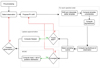 |
Fig. 8 Schematic of the semi-Bayesian approach, considering both an MCMC and Laplace approximation to characterise the posterior distribution. |
 |
Fig. 9 Comparison of the RV posterior distribution derived using the MCMC methodology (black curve) with the result of the Laplace approximation (dashed red line), for one observation of the M4 star considered in Sect. 2.3.2. |
4.2 Characterisation of the RV Posterior Distribution
We used the emcee package (Foreman-Mackey et al. 2013) to characterise the RV posterior probability distribution associated with each observation through the Markov chain Monte Carlo (MCMC) methodology. We assessed MCMC convergence through several criteria that must be met simultaneously: the chain length must be at least 50 times larger than the autocorrelation time (τ); the value of τ cannot change more than 1% after each iteration; the mean and standard deviation of the chains cannot change by more than 2% after each iteration.
Unfortunately, achieving convergence for a single ESPRESSO observation takes ~l0 min on a 24 cores@2.3 GHz and 128 GB RAM server, making the method computationally expensive for stars with a large number of available observations.
However, as the posterior distribution for the RV shift is approximately Gaussian (due to the large amount of information in the data), we can use the Laplace approximation to characterise it. By performing a second-order Taylor expansion around the posterior distribution maximum we can approximate the posterior with a Gaussian distribution centered at the mode of the posterior (also known as the maximum a posteriori (MAP)) and variance equal to the inverse of the Hessian of the log-posterior evaluated at the mode (e.g. see Sect. 3.4 of Rasmussen & Williams 2006), as shown in Fig. 9. In practice, this approximation transforms the characterisation of the posterior into an optimisation problem: the minimisation of the negative log likelihood (these are equivalent, because we assume a uniform prior for the RV). To solve this problem, we apply, once again, scipy’s implementation of the Brent method, reducing the computational time to ~30 s per observation on the same machine.
In order to compare RV estimates obtained through the MCMC methodology and the Laplace approximation we tested two targets, a K-type star with 27 ESPRESS018 observations and an M-type star with 21 ESPRESS019 observations, where ESPRESS018 and ESPRESS019 respectively refer to observations obtained before and after the ESPRESSO fiber link upgrade in June 2019 (Pepe et al. 2021). Figure 10 shows that the expected values for the RV shift obtained with the MCMC methodology and the Laplace approximation are, for both targets, within the respective uncertainties. The associated standard deviations are also in agreement at the cm s−1 level, given that they differ by ~2 cm s−1 at most, with mean and median differences smaller than 0.3 cm s−1, well below the expected 10 cm s−1 precision of ESPRESSO.
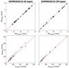 |
Fig. 10 Differences between the RV posterior distribution as characterised through the MCMC methodology and the Laplace approximation for 27 ESPRESS018 observations of a K-type star (left column) and 21 ESPRESS019 observations of an M-type star (right column). Top panel: comparison of the RV expected value in m s−1. We show, on each axis, the uncertainty associated with the corresponding measurement. Bottom: difference in the standard deviation of the RV posterior distribution between the two methodologies, in cm s−1. |
5 Results
In this section we show the results of the two template-based methodologies described above by comparing them against the CCF method and two other template matching methods. For this purpose, we use ESPRESSO data reduced with version 2.2.8 of the official pipeline5, and HARPS archival data reduced with version 3.5 of its official pipeline. We use 'classical' to refer to results obtained with the χ2 methodology discussed in Sect. 3, ‘S-BART’ to refer to those from the semi-Bayesian methodology (coupled with the Laplace approximation) from Sect. 4, and ‘DRS’ to refer to those from the CCF of the instrument pipeline. In order to assess the performance of our RV estimation methodologies, we start by comparing our results with those from HARPS-TERRA (Anglada-Escudé & Butler 2012) and SERVAL Zechmeister et al. (2018) using the same 22 HARPS observations of Barnard’s star. Subsequently, we focus our analysis on ESPRESSO data. In Sect. 5.2.2, we select one ESPRESSO target and create multiple stellar templates, each from a different number of observations, to evaluate the impact on the RV scatter and median RV uncertainty. In Sect. 5.2.3, we select 33 ESPRESSO GTO targets and compare the scatter and precision of the two template-based methodologies (classical and S–BART) with those from the ESO pipeline (CCF). In Sect. 5.2.4, we evaluate whether or not our RV uncertainties are consistent with the information present in the data by simulating stellar spectra from one of the available observations. Lastly, in Sect. 5.2.5 we use the same targets to estimate the nightly zero point (NZP) of the instrument with the three methodologies.
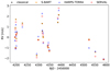 |
Fig. 11 RV time series for 22 observations of Barnard’s star corrected for the secular acceleration of the star. The black stars and orange crosses are RV estimates obtained with the classical and S–BART methodologies, respectively, with its own mean RV subtracted (for comparison purposes). The blue triangles and red dots are HARPS–TERRA and SERVAL RV estimates, respectively, also with their own mean RV subtracted. |
5.1 Validation with HARPS Data
In order to validate our algorithm by comparison to other template matching methods, we selected 22 HARPS observations of Barnard’s star (GJ699) obtained between April 4, 2007 and May 2, 2008, with program ID 072.C-0488(E). This set of observations was chosen as it is present in the introductory papers of the two pipelines chosen for this purpose (HARPS-TERRA and SERVAL) and the observations are publicly available.
In Fig. 11 we present the results obtained for HARPS–TERRA, SERVAL, and our two template matching methodologies. The HARP S-TERRA time series was obtained from Table 6 of Anglada-Escudé & Butler (2012)6 and we derived the SERVAL time series ourselves using the most recent public version of SERVAL7. For comparison purposes, we show all RV estimates after subtracting the RV mean with respect to each method. A visual comparison of the different time series allows to verify that the RV measurements show the same trends in all cases.
In Table 3 we compare the different methodologies with respect to the standard deviation of the RV estimates, a measure of scatter in the time series. We include the RV scatter reported in Zechmeister et al. (2018), as SERVAL-PAPER, for completeness. We find that both our methodologies reach the meter-per-second precision on HARPS data, achieving smaller scatter than with the HARPS–TERRA and SERVAL pipelines. The CCF-based HARPS pipeline leads to more scattered RV estimates, as expected given that Barnard’s star belongs to the M spectral class. We refrain from comparing the estimates for the RV uncertainties as the different template matching algorithms use different estimators for their calculation.
We find that our results are slightly less scattered than those obtained with other template matching methods. Despite the small differences, they are concordant with the others, suggesting that our methodologies are working as intended. The same decrease in RV scatter is found for our two template-based RV time series, suggesting that the different statistical framework is not the cause of the decrease. We believe the decrease to be due to differences in the way the stellar template is created and the telluric features are handled. In particular, S–BART attempts to minimise the impact of telluric features in RV estimation through a very conservative approach. This is achieved by creating a transmittance spectrum assuming the highest measured relative humidity amongst all observations of a given target, and then imposing a cut at 1% transmittance. Lastly, it should be noted that the difference in RV scatter between S–BART and HARP S–TERRA is equal to that between HARP S–TERRA and SERVAL.
Time-series RV scatter obtained with different template-based methodologies when applied to Barnard's star.
5.2 Application to ESPRESSO Data
In this section, we compare the performance of the CCF method of the ESO official pipeline with the application of the classical and S–BART methodologies when applied to ESPRESSO data.
5.2.1 Defining the Stellar Sample
Our analysis of the performance of template matching uses data collected during 2018, 2019, and early-2020 (until March). The selected targets are part of ESPRESSO’S blind RV survey program (Hojjatpanah et al. 2019; Pepe et al. 2021) and all have at least five observations that can be used to construct a stellar template. The fiber link of ESPRESSO was upgraded in June 2019 (Pepe et al. 2021), resulting in a change in the instrumental profile. We treat the data collected before and after the upgrade as if they were obtained from different instruments, that is, we create independent stellar templates for the data obtained before and after the technical intervention. We refer to data obtained before and after the fiber link upgrade as ‘ESPRESS018’ and ‘ESPRESS019’, respectively.
In order to assess the performance of our template-based approaches, we selected a sample of 33 targets, where 16 are M-type stars, 13 are K-type stars, and 4 are G-type stars. In total, we used approximately 1000 observations distributed between ESPRESS018 and ESPRESS019, as specified in Table 4.
The construction of the stellar template does not include any observation that has an airmass greater than 1.5, as discussed in Sect. 2.3.1. The selection of the targets in the sample was such that they all meet the condition discussed in Sect. 5.2.2 of having at least five observations that can be used in the construction of the stellar template.
Number of observations of each spectral type (ST) obtained before and after the fiber link upgrade of ESPRESSO.
5.2.2 The Impact of the Number of Observations in the Template
The first step to benchmark the performance of template-based RV estimation procedures with ESPRESSO data, and to understand for which targets we can take such an approach, is to evaluate the impact in the RV estimates of the number of observations used to construct the stellar template. For this purpose, from the sample described in Sect. 5.2.1, we selected 24 ESPRESS018 observations of an M-type star, from which we reserved the first 11 observations to construct stellar templates and used the other 13 to evaluate the performance of the templates. The 11 observations selected for the construction of the template cover a BERV region that starts at 25 km s−1 in the first observation, and ends at −19 km s−1 in the last one. The stellar templates are created by gradually selecting observations based on their BERV values after they have been sorted from largest to smallest. Each template is then used to compute RVs for the aforementioned set of 13 observations. We do not use the same data to construct the template and to evaluate the performance of the RV estimation methods so that templates constructed with a low number of observations are not too similar to the spectra used to construct them.
We find an improvement in both the scatter and median uncertainty reported by both our methodologies as the S/N of the template increases (Fig. 12). If we focus only on the RV scatter, we find no meaningful improvement with templates constructed from more than five observations. We therefore decided to estimate RVs only for targets that have at least five observations.
5.2.3 Comparison of the RV Scatter and Precision
We now compare the RV scatter and uncertainties obtained through the classical and S–BART methodologies. In order to achieve this, we apply both of our template matching algorithms to the roughly 1000 observations that compose our ESPRESSO sample (Sect. 5.2.1).
Similarly to other works, we find (Fig. 13 and Table 5) that the template-based methods, when applied to M-type stars, most often lead to a smaller scatter than the CCF method implemented in the DRS. This decrease is larger within the ESPRESS019 dataset (~10% smaller) than in the ESPRESS018 one (~8% smaller). For K-type stars, we find a similar decrease across the two datasets, of ~4%. Lastly, for G-type stars, the scatter both before and after the ESPRESSO fiber link upgrade is ~0.5% larger than the DRS, a result that should be taken with caution in light of the very limited sample size. The very similar RV estimates of the template matching methodologies were expected, as both use the same information, that is, the same spectral regions and the same model (the template).
We find very small differences – at the level of the cm s−1–between the median RV uncertainties from the S–BART and classical approaches. Figure 14 shows the histograms of the individual RV uncertainty estimates for the observations, which are separated by spectral type, for each ESPRESSO dataset, whilst Table 6 summarises the results. We see that for M-type stars, both template matching implementations yield a median RV uncertainty of ~13 cm s−1 smaller than with the ESPRESSO DRS, corresponding to almost half of the median CCF RV uncertainty. For K- and G-type stars, the gain in the median RV precision in comparison with the CCF is below 5 cm s−1.
We leave an analysis of the impact of differences in the levels of stellar activity on the RV estimates obtained using S–BART to a future study. Such a complex endeavour lays outside the scope of the current paper, and will require a complete analysis of the RV time series of each target, accounting for both stellar activity and (an unknown number of) planetary companions. It is also important to note that our current sample mostly contains stars with low levels of stellar activity (Hojjatpanah et al. 2019), meaning that we would either have to select a different stellar sample or be limited by that fact.
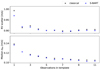 |
Fig. 12 Evolution of the RV scatter (top panel) and median uncertainty (bottom panel) with respect to 13 ESPRESS018 observations of an M-type star as a function of the number of spectra used to construct the template. The results from the classical methodology and the S–BART methodology are shown in black and blue, respectively. |
Mean ratio between the scatter of the RV time series as derived through the two template-based methodologies and the CCF-based ESPRESSO DRS, separated by spectral type, ST, and methodology.
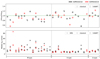 |
Fig. 13 Comparison of the results obtained with our template matching methodologies and with the CCF-based ESPRESSO DRS for ESPRESS018 (black) and ESPRESS019 (red) observations of the selected targets. Top panel: ratio of the rms in the template matching and DRS RV time series. The results from the classical and S–BART methods are represented by circles and diamonds, respectively. Bottom panel: median RV uncertainty for each target, as computed by the DRS (crosses), the classical approach (circle), and the S-BART method (diamonds). |
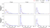 |
Fig. 14 Comparison of the RV uncertainties obtained for all ESPRESS018 (top panel) and ESPRESS019 (bottom panel) observations used in Fig. 13, separated by spectral type. The RV uncertainty estimated by the DRS is shown in blue while those estimated through the S-BART and classical methodologies are shown in black and red, respectively. |
5.2.4 Self-Consistency of RV Uncertainties
In order to determine whether or not our template matching estimates for the RV uncertainties are consistent with the information present in the spectra, we simulated spectra and analysed them with the different methodologies. The simulation process follows the following steps: (1) We start by selecting one reference observation. (2) For each pixel in the reference spectrum, we draw a random value from a Gaussian distribution with mean and standard deviation equal to the flux value and uncertainty of the reference spectrum, respectively. (3) We repeat the second step N = 100 times to build N ‘simulated’ spectra. (4) We apply the template matching algorithm using the stellar template that was built from the original data of the star whose observation was used as reference.
We created two datasets from two observations of an M5 star, one from ESPRESSO18 and another from ESPRESSO19, and compared the uncertainty associated with the RV value estimated for the reference spectrum with the RV scatter and median RV uncertainty for the simulated dataset, as shown in Table 7. We find that for the three methodologies, there is agreement between the RV uncertainty estimated for the original reference spectrum and the RV scatter and median uncertainty of the simulated datasets, even though the RV scatter and median uncertainties obtained with the CCF methodology for the assumed reference spectra are approximately double of those obtained with the S-BART and classical methods.
In addition to this analysis, we also made a comparison with the expected RV precision (Bouchy et al. 2001), as implemented in eniric (Neal & Figueira 2019), revealing that the median S-BART uncertainties from each spectral type are just a few cm s1 above the corresponding photon noise limit.
Comparison of the median RV uncertainties as obtained through the three methodologies, in cm s−1.
Results, in cm s−1, of the application of template matching and CCF to two simulated datasets where white noise was injected.
5.2.5 Nightly Zero-Point Variation
The final study that we did with ESPRESSO data was an analysis of the nightly zero point (NZP) of each RV estimation procedure, following the methodologies implemented in Courcol et al. (2015); Tal-Or et al. (2019). For our analysis, we again used the targets selected in Sect. 5.2.1 but, to enforce a balance of the number of observations between pre- and postfiber-link-upgrade data, we do not consider G-type stars, as we only have four targets, with the majority of observations taken before the fiber link upgrade (Table 4). Nonetheless, we still find that the ESPRESSO18 observations represent ~60% of our sample. It is important to note that our analysis uses a limited dataset that neither underwent a careful selection of targets nor had the contributions of stellar activity, planetary signals, and photon noise removed from the derived RVs. The subsequent results must therefore be taken as an upper bound for the achievable stability of ESPRESSO.
The NZP calculation starts with a subtraction of the error-weighted average from the time series of each target, thus centering all time-series around an RV of 0 m s−1. If a target has multiple observations in the same night, we replaced them by the median value. We computed the NZP for all nights in which at least three targets were observed. The NZP is calculated as the weighted average of the RVs, using weights equal to the inverse of the RV variances. The uncertainty in the NZP measurement is taken to be the maximum value between the propagated (through the weighted mean) RV uncertainty and the RV scatter of the night in question. For further details, we refer to Appendix A of the aforementioned articles.
The NZP time series is shown in Fig. 15, as derived from the RVs obtained with the ESPRESSO DRS as well as with our two template matching methodologies. First, it is important to note that we have a higher density of targets per night in ESPRESSO18 than we do in ESPRESSO19. When visually comparing the NZPs obtained with the different RV estimation methods, we find no significant differences, but an apparent smaller scatter in ESPRESSO19 data. This can be corroborated with a comparison of the weighted standard deviation of the NZPs (Table 8). We see that in both datasets, the template-based results have a slightly lower scatter than those from the DRS, with the classical approach yielding the smallest NZP scatter, particularly when applied to ESPRESSO18 data. A comparison of ESPRESSO18 and ESPRESSO19 data reveals a weighted variability about 10 cm s−1 across all methodologies, which is smaller in the latter dataset.
Despite the aforementioned limitations of our analysis, it is still noteworthy that, even under such circumstances, we find a NZP scatter below the meter-per-second threshold, both before and after the fiber link upgrade.
Weighted standard deviation, in cm s−1, of the derived NZPs for observations obtained before and after the 2019 ESPRESSO fiber link upgrade.
6 Limitations and Possible Improvements
The assumption that the stellar spectrum is invariant over time is a clear limitation in our template matching approaches, and is shared with other RV estimation procedures. We know that stellar activity induces spectral-line displacements and deformations that change with time. This will therefore induce a time-varying systematic error in the RV estimation, with a magnitude that is difficult to determine and that will depend on the star considered. This is a major obstacle in achieving precise RV estimates, that is, at the level of a few tens of centimeters. The solution will probably involve some form of data selection, namely at the spectral line level (Dumusque 2018; Cretignier et al. 2020), given that correctly modelling such complex effects seems a much more daunting task.
Even though the semi-Bayesian template matching methodology presented in Sect. 4 improves the RV estimation with respect to the classical template matching method, it has some shortcomings, which we are working on. First, the model for the spectra, effectively the prior with respect to the spectral fluxes, is built from the data to be analysed, which means that we are computing the likelihood of the data with respect to a model that was built using information from the same data. The most straightforward solution to this problem would be to reserve a set of spectra solely for the purpose of constructing the template, but at the cost of losing RV estimates at the times those spectra were acquired. Another way of tackling this problem would involve using a probabilistic model for the assumed time-invariant true spectrum. This could involve physically relevant information, as in the CCF method, and has been implemented to some degree in wobble (Bedell et al. 2019) and, using Gaussian Processes, in GRACE (Rajpaul et al. 2020).
Further, our semi-Bayesian approach depends on the classical implementation for the selection of the spectral orders to use as data. As discussed in the text, we are currently using those for which the classical template matching procedure was able to obtain results, that is, when our RV estimation convergence criteria were satisfied. However, it is possible that we could be discarding more (or less) information than we need to. One possible solution to this problem could be selection of orders through a maximisation of the information gain between the (Gaussian) RV posterior and the (uniform) RV prior using the Kullback-Leibler (KL) divergence (Kullback & Leibler 1951), which in this case is equivalent to minimising the RV uncertainty (standard deviation). Similarly to what is done in the classical procedure, this approach would have to select the orders for all available observations simultaneously, but now such selection involves the full RV results, not only those calculated at the level of the spectral order. Consequently, for targets with a large number of observations, this procedure is laborious and compounds a major computational burden.
The approximation of the RV posterior probability distribution by a Gaussian using the Laplace approximation may not be the best procedure in some cases. This method only uses the information around the MAP estimate to build the approximation and is consequently unable to account for any skewness in the posterior. A more complex technique, such as variational inference (for a detailed explanation, we refer to Gunapati et al. 2022; Blei et al. 2017), can use information from the entire posterior to build a more realistic approximation and is consequently more robust to skewness in the posterior.
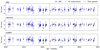 |
Fig. 15 Nightly zero point, shown as black dots, for each night when at least three different targets were observed. The date of the fiber link upgrade is highlighted with a dashed red line. The zero-centered RV of each target, observed in the night, is represented by a blue cross. The above were derived with results obtained with the following methodologies: ESPRESSO DRS (top); classical (middle); S-BART (bottom). |
7 Conclusions
In this work we revisit the template matching approach for RV estimation in a semi-Bayesian framework, which is implemented in a pipeline named S-BART: Semi-Bayesian Approach for RVs with Template matching. The key points of this approach can be summarised as: (i) First we create a high-S/N stellar template with at least five observations with an airmass smaller than 1.5; (ii) A common RV shift is then used to describe the differences between any given spectrum and a spectral template whose uncertainties are accounted for; (iii) The RV estimate and uncertainty are then determined as the mean and standard deviation of the RV posterior probability distribution, respectively; (iv) Due to the high computational cost of achieving convergence with an MCMC algorithm, we instead approximate the posterior with a Gaussian distribution, using the Laplace approximation.
We compared the results of this new method with those obtained with the CCF approach and with a classical implementation of the template matching algorithm, where independent RV shifts are assumed to describe the differences within each order between spectrum and template. The radial velocities are derived through the alignment of the spectra and a high-S/N template, in which the uncertainties of the data used to construct it are considered.
In order to validate and evaluate the performance of our algorithm, we applied it to observations from both HARPS and ESPRESSO, respectively. First, we compared the RV time series obtained with our template matching algorithms with those derived with the HARPS-TERRA and SERVAL pipelines, using 22 HARPS observations of Barnard’s star. Our two methodologies yield a time series with a scatter of ~14 cm s−1 smaller than that from SERVAL and ~8 cm s−1 smaller than that from HARPS-TERRA, revealing a good agreement between all RV estimates.
We then used S-BART to estimate RVs and the associated uncertainties for 33 ESPRESSO GTO targets of spectral types M, K, and G. The median ratio between the RMSs of the RVs obtained with our semi-Bayesian methodology and the CCF approach was 0.92 for M-type stars, 0.96 for K-type, and 1.03 for G-type for observations made before the ESPRESSO fiber link upgrade. After the upgrade we obtain a median ratio of 0.89, 0.96, and 1.06 for M, K, and G stars, respectively. The classical methodology also yields similar results to those obtained with the S-BART method. This shows that the two template matching approaches are able to provide more precise results for M-type stars, as one would expect, and also for K stars. Regarding the RVs uncertainties obtained with S-BART, we find a median value of ~14 cm s−1, ~8 cm s−1, ~11 cm s−1, for M-, K-, and G-type stars, respectively. We leave a more detailed analysis of the signals present in this sample to a future study, in which we plan to explore whether they are Keplerian or due to stellar activity.
Lastly, we also computed the NZP of the instrument, revealing a weighted NZP scatter of around 0.7 m s−1 for data obtained before the fiber link upgrade and 0.6 m s−1 after it. Even though the scatter is higher than the expected precision of ESPRESSO, the NZPs were calculated without removing stellar activity or planetary signals from the data and should therefore be taken as an upper limit of the obtainable precision.
Acknowledgements
The authors acknowledge the ESPRESSO project team for its effort and dedication in building the ESPRESSO instrument. This work was supported by FCT – Fundaçâo para a Ciência e a Tecnologia through national funds and by FEDER through COMPETE2020 – Pro-grama Operacional Competitividade e Inter-nacionalizaçâo by these grants: UID/FIS/04434/2019; UIDB/04434/2020; UIDP/04434/2020; PTDC/FIS-AST/32113/2017 & POCI-01-0145-FEDER-032113; PTDC/FIS-AST/28953/2017 & POCI-01-0145-FEDER-028953; PTDC/FIS-AST/28987/2017 & POCI-01-0145-FEDER-028987. A.M.S acknowledges support from the Fundaçâo para a Ciência e a Tecnologia (FCT) through the Fellowship 2020.05387. BD and POCH/FSE (EC). J.P.F. is supported in the form of a work contract funded by national funds through FCT with reference DL57/2016/CP1364/CT0005. S.G.S acknowledges the support from FCT through the contract nr. CEECIND/00826/2018 and POPH/FSE (EC). J.H.C.M. is supported in the form of a work contract funded by national funds through FCT (DL 57/2016/CP1364/CT0007). F.P.E. and C.L.O. would like to acknowledge the Swiss National Science Foundation (SNSF) for supporting research with ESPRESSO through the SNSF grants nr. 140649, 152721, 166227 and 184618. The ESPRESSO Instrument Project was partially funded through SNSF's FLARE Programme for large infrastructures. A.S.M., J.I.G.H. and R.R. acknowledge financial support from the Spanish Ministry of Science and Innovation (MICINN) project PID2020-117493GB-I00, and from the Government of the Canary Islands project ProID2020010129. J.I.G.H. also acknowledges financial support from the Spanish MICINN under 2013 Ramón y Cajal program RYC-2013-14875. This project has received funding from the European Research Council (ERC) under the European Union’s Horizon 2020 research and innovation programme (project FOUR ACES; grant agreement No 724427). It has also been carried out in the frame of the National Centre for Competence in Research PlanetS supported by the Swiss National Science Foundation (SNSF). DE acknowledges financial support from the Swiss National Science Foundation for project 200021_200726. H.M.T. and M.R.Z.O ackowledge financial support from the Agencia Estatal de Investigación of the Ministerio de Ciencia, Innovación y Universidades through projects PID2019-109522GB-C51. J.L-B. acknowledges financial support received from "la Caixa" Foundation (ID 100010434) and from the European Union’s Horizon 2020 research and innovation programme under the Marie Sklodowska-Curie grant agreement No 847648, with fellowship code LCF/BQ/PI20/11760023. R.A. is a Trottier Postdoctoral Fellow and acknowledges support from the Trottier Family Foundation. This work was supported in part through a grant from FRQNT. This work has been carried out within the framework of the National Centre of Competence in Research PlanetS supported by the Swiss National Science Foundation. The authors acknowledge the financial support of the SNSF. The INAF authors acknowledge financial support of the Italian Ministry of Education, University, and Research with PRIN 201278X4FL and the “Progetti Premiali” funding scheme. V.A. acknowledges the support from FCT through Investigador FCT contract nr. IF/00650/2015/CP1273/CT0001; N.J.N. acknowledges support form the following projects: CERN/FIS-PAR/0037/2019, PTDC/FIS-OUT/29048/2017; Based on data products from observations made with ESO Telescopes at the La Silla Paranal Observatory under programme ID 072.C-0488(E).
Appendix A Uncertainty Propagation in Cubic Splines
The cubic-spline interpolation used to calculate a value y at position x in the interval [xi, xi+1] can be written in the following form (p. 113 of Press 1992):
 (A.1)
(A.1)
where the double apostrophe represents the second derivative with respect to x and
 (A.2)
(A.2)
The computation of the second derivatives requires choosing proper boundary conditions. As discussed in Sect. 2.3.1 we remove the wavelength regions that are not common to all observations. Thus, as we do not interpolate in the edges, we can use natural boundary conditions, where the second derivative takes a value of zero at the edges of the input data. Following the notation of Press (1992) we can write down a general expression for the second derivatives:
 (A.3)
(A.3)
where h is a symmetric tridiagonal matrix given by:
 (A.4)
(A.4)
An expression for the propagation of uncertainties in cubic splines was derived in Gardner (2003), with the covariance between any two given interpolated points, u(ym, yn), given by:
 (A.5)
(A.5)

and where Uy is a N×N covariance matrix of the input data, ɡn is a column vector of length N with a 1 in the n-th column and 0 elsewhere, Qi is a column-vector of sensitivity coefficients of the second-derivatives in relation to the input values:
 (A.7)
(A.7)
In order to calculate the partial derivative (of the second derivatives) we start by selecting a given row from Equation A.3 and re-arranging the summation limits:
 (A.8)
(A.8)
The partial derivative then follows from Equation A.8:
 (A.9)
(A.9)
Special care must be taken due to the summation limits in Equation A.8, as not all terms in Equation A.9 exist for all indexes. As we are only interested in the variances of the interpolated values, i.e. we will not consider the effect of the covariances, we only have to evaluate Equation A.5 for the m = n case.
Lastly, as we are mainly dealing with ESPRESSO data, the computation of the second derivatives through Eq. A.3 implies the inversion of a matrix with size N − 2 × N − 2, with N = 9111, which represents a large computational burden. However, as we are dealing with a symmetric tridiagonal matrix of the form:
 (A.10)
where zn = yn, we can invert it with an explicit formula, using backwards continued fractions (Kılıç 2008):
 (A.11)
with  given by Eq 4 of the aforementioned paper:
 (A.12)
References
- Anglada-Escudé, G., & Butler, R. P. 2012, ApJS, 200, 15 [Google Scholar]
- Astudillo-Defru, N. 2015, PhD thesis, Université Grenoble, France [Google Scholar]
- Baranne, A., Queloz, D., Mayor, M., et al. 1996, A&AS, 119, 373 [NASA ADS] [CrossRef] [EDP Sciences] [Google Scholar]
- Bedell, M., Hogg, D.W., Foreman-Mackey, D., Montet, B. T., & Luger, R. 2019, AJ, 158, 164 [NASA ADS] [CrossRef] [Google Scholar]
- Bertaux, J. L., Lallement, R., Ferron, S., Boonne, C., & Bodichon, R. 2014, A&A, 564, A46 [NASA ADS] [CrossRef] [EDP Sciences] [Google Scholar]
- Blei, D. M., Kucukelbir, A., & McAuliffe, J. D. 2017, J. Am. Stat. Assoc., 112, 859 [CrossRef] [Google Scholar]
- Bouchy, F., Pepe, F., & Queloz, D. 2001, A&A, 374, 733 [NASA ADS] [CrossRef] [EDP Sciences] [Google Scholar]
- Courcol, B., Bouchy, F., Pepe, F., et al. 2015, A&A, 581, A38 [NASA ADS] [CrossRef] [EDP Sciences] [Google Scholar]
- Cretignier, M., Dumusque, X., Allart, R., Pepe, F., & Lovis, C. 2020, A&A, 633, A76 [NASA ADS] [CrossRef] [EDP Sciences] [Google Scholar]
- Cunha, D., Santos, N. C., Figueira, P., et al. 2014, A&A, 568, A35 [NASA ADS] [CrossRef] [EDP Sciences] [Google Scholar]
- Dumusque, X. 2018, A&A, 620, A47 [NASA ADS] [CrossRef] [EDP Sciences] [Google Scholar]
- Figueira, P., Pepe, F., Lovis, C., & Mayor, M. 2010, A&A, 515, A106 [NASA ADS] [CrossRef] [EDP Sciences] [Google Scholar]
- Figueira, P., Kerber, F., Chacon, A., et al. 2012, MNRAS, 420, 2874 [NASA ADS] [CrossRef] [Google Scholar]
- Flores, M., González, J. F., Arancibia, M. J., Buccino, A., & Saffe, C. 2016, A&A, 589, A135 [NASA ADS] [CrossRef] [EDP Sciences] [Google Scholar]
- Foreman-Mackey, D., Hogg, D. W., Lang, D., & Goodman, J. 2013, PASP, 125, 306 [Google Scholar]
- Gardner, J. 2003, J. Res. Natl. Inst. Standards Technol., 108, 69 [CrossRef] [Google Scholar]
- Gunapati, G., Jain, A., Srijith, P. K., & Desai, S. 2022, PASA, 39, e001 [NASA ADS] [CrossRef] [Google Scholar]
- Hojjatpanah, S., Figueira, P., Santos, N. C., et al. 2019, A&A, 629, A80 [NASA ADS] [CrossRef] [EDP Sciences] [Google Scholar]
- Hsu, D. C., Ford, E. B., Ragozzine, D., & Ashby, K. 2019, AJ, 158, 109 [NASA ADS] [CrossRef] [Google Scholar]
- Kılıç, E. 2008, Appl. Math. Comput., 197, 345 [Google Scholar]
- Kuerster, M., Endl, M., Rouesnel, F., et al. 2003, A&A, 403, 1077 [NASA ADS] [CrossRef] [EDP Sciences] [Google Scholar]
- Kullback, S., & Leibler, R. A. 1951, Annal. Math. Stat., 22, 79 [CrossRef] [Google Scholar]
- Lafarga, M., Ribas, I., Lovis, C., et al. 2020, A&A, 636, A36 [NASA ADS] [CrossRef] [EDP Sciences] [Google Scholar]
- Marconi, A., Abreu, M., Adibekyan, V., et al. 2021, The Messenger, 182, 6 [Google Scholar]
- Mayor, M., & Queloz, D. 1995, Nature, 378, 355 [Google Scholar]
- Mayor, M., Marmier, M., Lovis, C., et al. 2011, ArXiv eprints [arXiv:1109.2497] [Google Scholar]
- Mayor, M., Lovis, C., & Santos, N. C. 2014, Nature, 513, 328 [Google Scholar]
- Neal, J., & Figueira, P. 2019, J. Open Source Softw., 4, 1053 [NASA ADS] [CrossRef] [Google Scholar]
- Pepe, F., Mayor, M., Galland, F., et al. 2002, A&A, 388, 632 [NASA ADS] [CrossRef] [EDP Sciences] [Google Scholar]
- Pepe, F., Cristiani, S., Rebolo, R., et al. 2021, A&A, 645, A96 [NASA ADS] [CrossRef] [EDP Sciences] [Google Scholar]
- Press, W. H. 1992, Numerical Recipes in C: The Art of Scientific Computing, 2nd edn. (Cambridge: Cambridge University Press) [Google Scholar]
- Rainer, M., Borsa, F., & Affer, L. 2020, Exp. Astron., 49, 73 [Google Scholar]
- Rajpaul, V. M., Aigrain, S., & Buchhave, L. A. 2020, MNRAS, 492, 3960 [NASA ADS] [CrossRef] [Google Scholar]
- Rasmussen, C. E., & Williams, C. K. I. 2006, Gaussian Processes for Machine Learning, Adaptive Computation and Machine Learning (Cambridge, Mass: MIT Press) [Google Scholar]
- Rauer, H., Catala, C., Aerts, C., et al. 2014, Exp. Astron., 38, 249 [Google Scholar]
- Robertson, P., Bender, C., Mahadevan, S., Roy, A., & Ramsey, L. W. 2016, ApJ, 832, 112 [CrossRef] [Google Scholar]
- Rosenthal, L. J., Fulton, B. J., Hirsch, L. A., et al. 2021, ApJS, 255, 8 [NASA ADS] [CrossRef] [Google Scholar]
- Schmelling, M. 1995, Phys. Scr., 51, 676 [CrossRef] [Google Scholar]
- Tal-Or, L., Trifonov, T., Zucker, S., Mazeh, T., & Zechmeister, M. 2019, MNRAS, 484, L8 [Google Scholar]
- Virtanen, P., Gommers, R., Oliphant, T. E., et al. 2020, Nat. Methods, 17, 261 [Google Scholar]
- Wehbe, B., Cabral, A., Figueira, P., & Avila, G. 2019, in Fourth International Conference on Applications of Optics and Photonics, ed. M. F. P. Martins Costa (Lisbon, Portugal: SPIE), 65 [CrossRef] [Google Scholar]
- Zechmeister, M., Reiners, A., Amado, P. J., et al. 2018, A&A, 609, A12 [NASA ADS] [CrossRef] [EDP Sciences] [Google Scholar]
Publicly available in https://github.com/iastro-pt/sBART
https://github.com/mzechmeister/serval; commit d31a918.
All Tables
Central wavelength (measured in air) and size of the spectral regions removed from the spectra.
Analysis of the S/N between each of the two templates and three different subsets of the available observations.
Time-series RV scatter obtained with different template-based methodologies when applied to Barnard's star.
Number of observations of each spectral type (ST) obtained before and after the fiber link upgrade of ESPRESSO.
Mean ratio between the scatter of the RV time series as derived through the two template-based methodologies and the CCF-based ESPRESSO DRS, separated by spectral type, ST, and methodology.
Comparison of the median RV uncertainties as obtained through the three methodologies, in cm s−1.
Results, in cm s−1, of the application of template matching and CCF to two simulated datasets where white noise was injected.
Weighted standard deviation, in cm s−1, of the derived NZPs for observations obtained before and after the 2019 ESPRESSO fiber link upgrade.
All Figures
|
Fig. 1 Workflow of the processing stage that we apply before the RV estimation. |
| In the text | |
|
Fig. 2 Comparison between the telluric spectrum obtained from Tapas (black), with the continuum level obtained with a median filter (dashed blue line), and the telluric threshold (dotted red line) built from the continuum, for three spectral regions. |
| In the text | |
|
Fig. 3 BERV-corrected spectra of different observations at the start (top) and end (bottom) of a spectral order. Top panel: dashed red line represents the minimum wavelength, so that all (of the presented) orders have data at the start of the order. Bottom panel: dashed red line represents the last wavelength at which all orders have data. |
| In the text | |
|
Fig. 4 Histogram of the S/N, for the 100th order, of the template and each of the 21 individual observations of an M4 star, obtained after the fiber link upgrade of ESPRESSO in mid-2019. In order to compare the impact of the number of observations used to construct the template on its associated uncertainty, one template was built with 8 observations (black curve) and the other with 13 observations (blue curve), selected by the airmass at the start of each observation. For all observations we also highlight the comparison with observations with a S/N of at least 100 for the selected spectral order by filling the bins with the corresponding colour. |
| In the text | |
|
Fig. 5 Outlier removal routine for two regions of the same order, with respect to an observation for which outlier identification achieved convergence after the first iteration. For representation purposes, we normalized the flux in the center and the edge of the order. Top row: comparison between the stellar template (red line) and the spectra (black line). The blue crosses represent the points that were flagged by the method. Bottom row: differences between the template and spectra (black points). The blue line is the median value, whilst the dotted red lines represent a 6σ difference from it. |
| In the text | |
|
Fig. 6 Schematic of the classical template matching RV-estimation procedure, including the computation of the uncertainties in the stellar template. We iterate over orders at the highest level, and not observations, in order to optimise the computational efficiency of the method. |
| In the text | |
|
Fig. 7 The χ2 curve for the 100th spectral order of an ESPRESSO observation of GJ699 (black line), sampled with a step of 10 cm s−1 inside the 200 m s−1 search window centered on the ESPRESSO DRS estimate. The parabolic fit is shown as the red line. The red circles represent the RV estimates provided by the Brent method before meeting the convergence criteria. The dashed blue line is the final RV, calculated with Eq. (3), and the dotted green line the ESPRESSO DRS estimate for the given observation. |
| In the text | |
|
Fig. 8 Schematic of the semi-Bayesian approach, considering both an MCMC and Laplace approximation to characterise the posterior distribution. |
| In the text | |
|
Fig. 9 Comparison of the RV posterior distribution derived using the MCMC methodology (black curve) with the result of the Laplace approximation (dashed red line), for one observation of the M4 star considered in Sect. 2.3.2. |
| In the text | |
|
Fig. 10 Differences between the RV posterior distribution as characterised through the MCMC methodology and the Laplace approximation for 27 ESPRESS018 observations of a K-type star (left column) and 21 ESPRESS019 observations of an M-type star (right column). Top panel: comparison of the RV expected value in m s−1. We show, on each axis, the uncertainty associated with the corresponding measurement. Bottom: difference in the standard deviation of the RV posterior distribution between the two methodologies, in cm s−1. |
| In the text | |
|
Fig. 11 RV time series for 22 observations of Barnard’s star corrected for the secular acceleration of the star. The black stars and orange crosses are RV estimates obtained with the classical and S–BART methodologies, respectively, with its own mean RV subtracted (for comparison purposes). The blue triangles and red dots are HARPS–TERRA and SERVAL RV estimates, respectively, also with their own mean RV subtracted. |
| In the text | |
|
Fig. 12 Evolution of the RV scatter (top panel) and median uncertainty (bottom panel) with respect to 13 ESPRESS018 observations of an M-type star as a function of the number of spectra used to construct the template. The results from the classical methodology and the S–BART methodology are shown in black and blue, respectively. |
| In the text | |
|
Fig. 13 Comparison of the results obtained with our template matching methodologies and with the CCF-based ESPRESSO DRS for ESPRESS018 (black) and ESPRESS019 (red) observations of the selected targets. Top panel: ratio of the rms in the template matching and DRS RV time series. The results from the classical and S–BART methods are represented by circles and diamonds, respectively. Bottom panel: median RV uncertainty for each target, as computed by the DRS (crosses), the classical approach (circle), and the S-BART method (diamonds). |
| In the text | |
|
Fig. 14 Comparison of the RV uncertainties obtained for all ESPRESS018 (top panel) and ESPRESS019 (bottom panel) observations used in Fig. 13, separated by spectral type. The RV uncertainty estimated by the DRS is shown in blue while those estimated through the S-BART and classical methodologies are shown in black and red, respectively. |
| In the text | |
|
Fig. 15 Nightly zero point, shown as black dots, for each night when at least three different targets were observed. The date of the fiber link upgrade is highlighted with a dashed red line. The zero-centered RV of each target, observed in the night, is represented by a blue cross. The above were derived with results obtained with the following methodologies: ESPRESSO DRS (top); classical (middle); S-BART (bottom). |
| In the text | |
Current usage metrics show cumulative count of Article Views (full-text article views including HTML views, PDF and ePub downloads, according to the available data) and Abstracts Views on Vision4Press platform.
Data correspond to usage on the plateform after 2015. The current usage metrics is available 48-96 hours after online publication and is updated daily on week days.
Initial download of the metrics may take a while.