| Issue |
A&A
Volume 687, July 2024
|
|
|---|---|---|
| Article Number | A120 | |
| Number of page(s) | 17 | |
| Section | Extragalactic astronomy | |
| DOI | https://doi.org/10.1051/0004-6361/202348072 | |
| Published online | 02 July 2024 | |
Heavily obscured AGN detection: A radio versus X-ray challenge
1
Dipartimento di Fisica e Astronomia, Università di Bologna, Via Gobetti 93/2, 40129 Bologna, Italy
2
INAF – Osservatorio di Astrofisica e Scienza dello Spazio di Bologna, Via Gobetti 93/3, 40129 Bologna, Italy
e-mail: This email address is being protected from spambots. You need JavaScript enabled to view it.
3
Department of Physics and Astronomy, Clemson University, Kinard Lab of Physics, Clemson, SC 29634, USA
4
INAF – Istituto di Radioastronomia, Via Gobetti 101, 40129 Bologna, Italy
5
INAF – Osservatorio Astrofisico di Arcetri, Largo Enrico Fermi 5, 50125 Firenze, Italy
6
Institut de Ciències del Cosmos (ICCUB), Universitat de Barcelona (IEEC-UB), Martí i Franquès, 1, 08028 Barcelona, Spain
7
ICREA, Pg. Luís Companys 23, 08010 Barcelona, Spain
8
Space Telescope Science Institute, 3700 San Martin Drive, Baltimore, MD 21218, USA
9
Department of Physics and Astronomy, Johns Hopkins University, Baltimore, MD 21218, USA
Received:
26
September
2023
Accepted:
29
January
2024
Abstract
Context. In the supermassive black hole (SMBH)-galaxy coevolution scenario, heavily obscured active galactic nuclei (AGN) represent a fundamental phase of SMBH growth during which most of the BH mass is accreted and the scaling relations with the host galaxy are set. Obscured nuclei are thought to constitute a major fraction of the whole AGN population, but their statistics and evolution across cosmic time are still highly uncertain. Therefore, it is pivotal to identify new ways to detect this vast and hidden population of growing SMBHs. A promising way to select heavily obscured AGN is through radio emission, which is largely unaffected by obscuration and can be used as a proxy for nuclear activity.
Aims. In this work, we study the AGN radio detection effectiveness in the major deep extragalactic surveys, considering different AGN obscuration levels, redshift, and AGN bolometric luminosities. We particularly focus on comparing their radio and X-ray detectability, making predictions for present and future radio surveys.
Methods. We extrapolated the predictions of the AGN population synthesis model of the cosmic X-ray background (CXB) to the radio band, by deriving the 1.4 GHz luminosity functions of unobscured (i.e., with hydrogen column densities log NH < 22), obscured (22 < log NH < 24), and Compton-thick (CTK, log NH > 24) AGN. We then used these functions to forecast the number of detectable AGN based on the area, flux limit, and completeness of a given radio survey and compare it with the AGN number resulting from X-ray predictions.
Results. When applied to deep extragalactic fields covered both by radio and X-ray observations, we show that, while X-ray selection is generally more effective in detecting unobscured AGN, the surface density of CTK AGN radio detected is on average ten times larger than the X-ray one, and even greater at high redshifts, considering the current surveys and facilities. Our results suggest that thousands of CTK AGN are already present in current radio catalogs, but most of them escaped any detection in the corresponding X-ray observations. We also present expectations for the number of AGN to be detected by the Square Kilometer Array Observatory (SKAO) in its future deep and wide radio continuum surveys, finding that it will be able to detect more than 2000 AGN at z > 6 and tens of them at z > 10, more than half of which are expected to be CTK.
Key words: galaxies: active / galaxies: evolution / galaxies: luminosity function, mass function / radio continuum: galaxies
© The Authors 2024
 Open Access article, published by EDP Sciences, under the terms of the Creative Commons Attribution License (https://creativecommons.org/licenses/by/4.0), which permits unrestricted use, distribution, and reproduction in any medium, provided the original work is properly cited.
This article is published in open access under the Subscribe to Open model. This email address is being protected from spambots. You need JavaScript enabled to view it. to support open access publication.
1. Introduction
Obscured active galactic nuclei (AGN) are important astrophysical sources in the context of the supermassive black hole (SMBH)-galaxy coevolution scenario (Hickox & Alexander 2018; Hopkins et al. 2008). In this framework, most SMBH and galaxy growth occurs during a very active obscured phase of BH accretion and star formation (SF). The radiative and kinetic energy released by the AGN is then supposed to sweep away the obscuring material, eventually quenching both SF and SMBH growth (Lapi et al. 2018). A number of results from deep X-ray surveys indicate that the role of obscured and heavily obscured AGN might be particularly important at high redshift. Vito et al. (2018) showed that the fraction of AGN obscured by gas column densities (NH) larger than log NH > 23 increases up to ∼80% at z ∼ 4, as also supported by analytical models and simulations (Ni et al. 2020; Lapi et al. 2020; Gilli et al. 2022b). Furthermore, the SMBH accretion rate density (BHARD) derived by different coevolutionary models (Volonteri & Reines 2016; Sijacki et al. 2015; Shankar et al. 2014) is in good agreement with the observational results at least up to z < 3, whereas at larger redshifts the models seem to overpredict the BHARD derived from X-ray surveys. While it is not clear yet whether issues in the simulations are responsible for this overprediction (Vito et al. 2016), one of the most widely proposed solutions is the existence of a highly obscured AGN population at high redshifts, which has been missed by X-ray surveys (Barchiesi et al. 2021).
JWST is pushing the frontier of the spectroscopic identification of obscured AGN well into the epoch of the reionization, enabling us to look at the primordial stages of the SMBH and galaxy formation. Very recent results coming from JWST observations (Maiolino et al. 2023; Greene et al. 2024) show a surprisingly high number density of broad-line (BL) AGN among the population of high-z compact red sources, which usually lack any X-ray detection even in deep X-ray fields (Übler et al. 2023). In Yang et al. (2023), the identification of high-z obscured AGN using the reddest JWST filters led to a BHARD substantially higher than the X-ray results for z > 3, suggesting that we are probably still missing the bulk of the AGN population at these redshifts.
Therefore it is of primary importance to detect and identify obscured Compton-thin (22 < log NH < 24) and Compthon-thick (CTK; log NH > 24) AGN, to understand their role in SMBH-galaxy coevolution and to constrain their physical properties and demographics, especially in the early Universe.
Among the several approaches reported in the literature to select AGN, the most commonly used are: X-ray selection (Ranalli et al. 2005), near-infrared (NIR) and mid-infrared (MIR) color selection (Donley et al. 2012), spectral energy distribution (SED) fitting (Boquien et al. 2019; Yang et al. 2020; Brammer et al. 2008), spectroscopic classification (Mignoli et al. 2013), and deviation from the far-infrared-radio-correlation of star-forming galaxies (SFGs; Novak et al. 2017; Delvecchio et al. 2017, 2021).
The first three diagnostics are normally used to select moderate-to-high luminosity AGN (HLAGN), which are radiatively efficient AGN usually characterized by bolometric luminosities larger than Lbol > 1043 erg s−1. However, when heavily obscured AGN are taken into account, the effectiveness of X-ray and NIR-MIR selections shows severe limitations.
AGN obscuration is produced by dust and gas close to the central SMBH (the torus, in the inner parsec), but also by the cold interstellar medium (ISM) of the host galaxy (Aravena et al. 2020; Decarli et al. 2023; Lusso et al. 2023). While optical emission is generally absorbed by dust, X-ray emission can penetrate through moderate-to-large gas column densities. However, the X-ray detection of CTK AGN is challenging: for these objects, the X-ray emission in the energy range 0.5–10 keV is almost completely absorbed by gas, and only very high energy X-ray photons (> 10 keV) can escape. Moreover, X-ray selection suffers from the limited area-sensitivity combination of current X-ray facilities (Gilli et al. 2022a), making the detection of the faintest sources even harder.
Different NIR-MIR color selection techniques proved to be effective in selecting obscured AGN by detecting the emission from their warm dusty torus (Stern et al. 2012; Assef et al. 2013; Donley et al. 2012). However, the fraction of contaminants (mainly dusty SFG) that mimic the colors of obscured AGN increases at high redshift, particularly for those selections relying on NIR photometric bands (Donley et al. 2012). Therefore, applying a cut in redshift (z < 3) is usually necessary to provide reliable selections. Furthermore, NIR-MIR color prescriptions need a strong AGN component; hence, systems with weak AGN emission are not easily identified (Hickox & Alexander 2018).
Radio emission can uncover low-luminosity AGN, that do not show the strong signatures of HLAGN, and with less time-demanding observations compared to spectroscopy or X-ray. A great advantage of radio emission is that it is largely unaffected by AGN obscuration since both gas and dust opacities are almost negligible at typical radio frequencies (e.g., 1.4 GHz, Hildebrand 1983).
Historical radio surveys were mostly sensitive to the powerful (L1.4 GHz > 1025 W Hz−1) population of the so-called radio-loud (RL) AGN (White et al. 1997; Becker et al. 1995, 2001), for which a significant fraction of the power produced by the accretion process is released in kinetic form through the formation of relativistic jets that may expand up to the Mpc scales. However, new-generation radio surveys (Heywood et al. 2020; Alberts et al. 2020; van der Vlugt et al. 2021; Hale et al. 2023) are deep enough to detect also SFG and so-called radio-quiet (RQ) AGN, which are radiatively efficient AGN with much weaker radio emission, typically confined on (sub)kiloparsec scales. In particular, reaching μJy sensitivities, it is possible to detect radio luminosities down to L1.4 GHz ∼ 1023 W Hz−1 (corresponding to νLν ∼ 1023 erg s−1; with ν = 1.4 GHz) and star-formation rates SFR ∼ 100 M⊙ yr−1 up to z ∼ 3.
At frequencies around a few GHz, the radio emission is, both for AGN and SFG, mostly due to optically thin synchrotron radiation, emitted by electrons accelerated to relativistic velocities by different acceleration mechanisms. In SFG the acceleration is provided by supernova explosions in SF regions, while in RL AGN the expanding radio jets originate from the interaction of the electrons with the strong magnetic field amplified by the SMBH accretion disk (Blandford & Znajek 1977). In RQ AGN, multiple mechanisms may be at work. Radio emission can be associated with circumnuclear SF regions, small (sub)kiloparsec scale jets, and/or other AGN-related mechanisms, such as shocked radiative winds or coronal winds (see Panessa et al. 2019, for a comprehensive review). A way to distinguish between SF or AGN-related radio emission is provided by the well-known Far Infrared Radio Correlation (Novak et al. 2017; Delvecchio et al. 2021). This relation arises because the same population of massive stars that heats up dust, causing it to reradiate its energy in the far-infrared (FIR), produces supernovae that generate relativistic particles emitting synchrotron radiation at radio frequencies. This correlation is quantified by a parameter qTIR = log(LTIR)/log(L1.4 GHz), namely the ratio between the total IR luminosity integrated between 8–1000μm and the 1.4 GHz luminosity. This correlation has been found to depend both on the redshift and the stellar mass (M*) of the sources (Delhaize et al. 2017; Delvecchio et al. 2017, 2021). Galaxies with radio emission in excess of what is predicted by the FIR-radio correlation likely possess an AGN-driven radio component, independently of which exact mechanism is responsible for it. It is common to indicate these sources as Radio-Excess (REX) AGN1 (Delvecchio et al. 2017; Nandra & Iwasawa 2007).
In this work we aim to investigate the effectiveness of selection methods based on radio and X-ray emission considering AGN at different levels of obscuration and at different intrinsic luminosities and redshift, focusing particularly on CTK AGN. In Sect. 2 we translate the AGN X-ray luminosity functions into the radio band (1.4 GHz) and predict the number of detectable AGN over a radio field, given its depth, area, and completeness corrections. In Sect. 3 we present the 1.4 GHz luminosity function (Sect. 2.2), radio number counts (Sect. 3.2) and AGN predictions (Sect. 3.3), comparing the results with those in the literature. In Sect. 4 we apply our model to the major extragalactic fields covered by X-ray and radio observations, discussing for which type of AGN the 1.4 GHz emission performs better than the X-ray one. In Sect. 4.3, we focus on the predictions for the high-redshift Universe (z > 3), while in Sect. 4.4 we present the expectations for the Square Kilometer Array Observatory (SKAO) surveys that will be done in the next future.
We assume a flat ΛCDM universe with H0 = 70 km s−1 Mpc−1, Ωm = 0.3, ΩΛ = 0.7, Ωk = 0.
We assume AGN radio spectra of the form Sν ∝ ν−α, with α = 0.7, which is the typical spectral slope considered for extragalactic synchrotron emission (Smolčić et al. 2017b; Novak et al. 2017). When L1.4 GHz is reported we refer to νLν (with ν = 1.4 GHz), in units of erg s−1.
2. Methods
Cosmic X-ray background (CXB) models (Gilli et al. 2007; Ueda et al. 2014; Buchner et al. 2015; Ananna et al. 2019), by studying the integrated X-ray emission of faint extragalactic point-like sources, can provide an AGN census for any obscuration level and to include also the most CTK AGN population, poorly sampled even in the deepest X-ray surveys. The different CXB models almost agree in predicting a consistent fraction of CTK AGN among the whole AGN population, that is between 30 − 50%.
To derive the AGN radio luminosity function (RLF) we followed the approach described in the following sections which is based on the CXB model of Gilli et al. (2007; G07 hereafter) and considers the AGN radio-hard-X luminosity relation (L1.4 GHz−LHX) derived by D’Amato et al. (2022).
A similar approach was also followed in Ballantyne (2009) and in La Franca et al. (2010), the latter to investigate the global AGN kinetic energy release in the context of AGN feedback processes.
2.1. Hard-X luminosity function
The CXB model in G07 considers for the unobscured AGN population the soft-X-ray luminosity function (SXLF, energy range: 0.5–2 keV) derived by Hasinger et al. (2005), of the form:
![Mathematical equation: $$ \begin{aligned} \frac{\mathrm{d}\Phi (L_{\rm X},z)}{\mathrm{d} L_{\rm X}}=A\biggl [\biggl (\frac{L_{\rm X}}{L_*}\biggr )^{\gamma _1}+\biggl (\frac{L_{\rm X}}{L_*}\biggr )^{\gamma _2}\biggr ]^{-1} \cdot e_z(z,L_{\rm X}) \cdot e_{\rm decl}(z), \end{aligned} $$](/articles/aa/full_html/2024/07/aa48072-23/aa48072-23-eq1.gif) (1)
(1)
where the values of the normalization A, of the characteristic luminosity L*, and of γ1, γ2 are taken from Table 5 of Hasinger et al. (2005). The evolution factor ez was derived in Hasinger et al. (2005) considering a luminosity-dependent evolution model. The term edecl:
![Mathematical equation: $$ \begin{aligned} e_{\rm decl}(z) = {\left\{ \begin{array}{ll} 1 \quad \text{ for} \quad z<2.7 \\ 10^{[-0.43\cdot (z-2.7)]}\quad \text{ for} \quad z\ge 2.7 \end{array}\right.} \end{aligned} $$](/articles/aa/full_html/2024/07/aa48072-23/aa48072-23-eq2.gif) (2)
(2)
is introduced to reproduce the steep decline in the density of AGN observed at high-z (e.g. Brusa et al. 2009).
Following the same approach as in G07, we obtain the corresponding Hard-X luminosity function (HXLF, energy range: 2–10 keV) assuming a Gaussian distribution of X-ray spectral indices centered at Γ = 1.9 (Piconcelli et al. 2005). Then, using the obscured-to-unobscured AGN ratio in G07, we derive the HXLF of the different subpopulations of AGN in terms of their level of obscuration. In particular, we derive the HXLF of obscured Compton-thin and CTK AGN, the latter assumed to have the same number density of the obscured Compton-thin AGN. The orange solid line in Fig. 1 corresponds to the total HXLF at z = 0, computed by summing the luminosity functions of all the subpopulations of obscured and unobscured AGN.
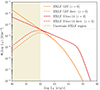 |
Fig. 1. HXLF of all AGN obtained following the prescription of the CXB model in G07 and computed at z = 0 (solid orange line). The dashed orange line is the same HXLF but introducing a cutoff at log LX < 42, where the HXLF measurements are most uncertain. The red curve represents the HXLF as derived by Vito et al. (2014), computed at z = 3, and implemented as the baseline model for z > 3. The dashed red line is the Vito et al. (2014) HXLF with the same cutoff described above. |
The faint end of the XLF is poorly observationally constrained for values of log LX ≤ 42, since at these X-ray luminosities it is difficult to distinguish between the X-ray emission coming from AGN and that coming from SF processes in normal galaxies. To derive information in the faintest AGN luminosity regime (log LX ≤ 42), X-ray luminosity functions are usually extrapolated using the steep slopes determined at brighter luminosities, but the possibility that they remain constant or even decline cannot be excluded. Consequently, we introduced a cut-off in the Hasinger et al. (2005) SXLF at log LX < 42:
![Mathematical equation: $$ \begin{aligned} \frac{\mathrm{d}\Phi (L_{\rm X},z)}{\mathrm{d} L_{\rm X}}=A\biggl [\biggl (\frac{L_{\rm X}}{L_*}\biggr )^{\gamma _1}+\biggl (\frac{L_{\rm X}}{L_*}\biggr )^{\gamma _2}+\biggl (\frac{L_{\rm X}}{L_1}\biggr )^{\gamma _3}\biggr ]^{-1} \cdot e_z(z,L_{\rm X}) \cdot e_{\rm decl}(z), \end{aligned} $$](/articles/aa/full_html/2024/07/aa48072-23/aa48072-23-eq3.gif) (3)
(3)
where L1 = 1040 erg s−1 and γ3 = −1 (see orange dashed line in Fig. 1).
Furthermore, since the X-ray luminosity function of Hasinger et al. (2005) was largely derived from AGN samples at z < 3, we also considered the high-z X-ray luminosity function presented in Vito et al. (2014). In this work the authors, assembling a sample of 141 AGN at 3 < z < 5 from X-ray surveys of different sizes and depths, built an HXLF specific for high-z AGN. In our work, we used the Vito et al. (2014) results as baseline HXLF at z > 3. In Vito et al. (2014) HXLF we assumed a constant obscured AGN fraction with luminosity and a number ratios between unobscured, obscured Compton-thin, and obscured Compton-thick AGNs of 1:4:4. Both these assumptions are in agreement with the observational results reported in Vito et al. (2018). The total HXLF is presented in red in Fig. 1 at z = 3 (red solid line) and has the following analytic expression:
![Mathematical equation: $$ \begin{aligned} \frac{\mathrm{d}\Phi (L_{\rm X},z)}{\mathrm{d} L_{\rm X}}=A\biggl [\biggl (\frac{L_{\rm X}}{L_s}\biggr )^{\gamma _a}+\biggl (\frac{L_{\rm X}}{L_s}\biggr )^{\gamma _b}\biggr ]^{-1} \cdot \bar{e}_z(z,L_{\rm X}), \end{aligned} $$](/articles/aa/full_html/2024/07/aa48072-23/aa48072-23-eq4.gif) (4)
(4)
where the values of the parameters Ls, γa, γb, are taken from Table 5 in Vito et al. (2014) and the redshift evolution factor,  is given by Eq. (7) of the same work. The HXLF derived in Vito et al. (2014) provides a very good description of the high-z obscured AGN fraction and AGN space density measured in the 2Ms CDFN and 7Ms CDFS (see Vito et al. 2018).
In conclusion, our baseline model uses the HXLF derived by the CXB model in G07 for z < 3 and of the HXLF of Vito et al. (2014) one for z > 3. To account for the uncertainty on the X-ray luminosity function faint end also at high-z, we applied to the Vito et al. (2014) HXLF the same cut-off ((LX/L1)γ3) reported in Eq. (3) (see red dashed line in Fig. 1).
2.2. Predicted AGN radio luminosity function
To convert the HXLF into a RLF requires a relation between AGN luminosities in the two bands (e.g. Panessa et al. 2015; Merloni et al. 2003; Dong et al. 2021). In this work, we assume the relation of D’Amato et al. (2022), that was derived using the deep radio and X-ray data available in the ∼ 0.2 deg−2 field centered on the quasar SDSS J1030+0524 (hereafter J1030):
 (5)
(5)
This relation was computed from a sample of X-ray selected AGN and early-type galaxies (ETG), spectroscopically confirmed up to z ∼ 3, spanning a wide range of luminosities. The 2–10 keV luminosities cover the range log LHX ∈ [40.5, 45], while the radio luminosities extend over log L1.4 GHz ∈ [37,43]. Radio upper limits were taken into account using survival analysis. Since the relation was computed using X-ray selected sources, and since we started from an X-ray luminosity function, this relation is perfectly suited for our aim. Furthermore, since the sample of D’Amato et al. (2022) includes sources up to z ∼ 3, their relation extends well beyond the local universe, as opposed to other L1.4 GHz−LHX relations in the literature.
The relation of D’Amato et al. (2022) does not consider any prior selection in the radio loudness parameter of the sources, but 83% of the sample (87% accounting radio upper limits) is radio quiet according to the radio loudness threshold RX = log(L1.4 GHz/LHX) < −3.5, originally defined in Terashima & Wilson (2003). The relation derived from D’Amato et al. (2022) differs significantly from those found in the literature for RL AGN (e.g. Fan & Bai 2016). This means that the RL AGN population cannot be described by this relation and they will not be included in our predictions (see Sect. 3).
To transform the HXLF into a RLF we considered a Gaussian probability distribution function that returns the probability P that an AGN with a 2–10 keV luminosity LHX has a radio luminosity L1.4 GHz according to the D’Amato et al. (2022) L1.4 GHz−LHX relation:
 (6)
(6)
 (7)
(7)
where the Gaussian dispersion σR = 0.5 is given by the intrinsic dispersion of the L1.4 GHz−LHX relation. Then, we computed the RLF by weighing the HXLF by the probability distribution computed above:
 (8)
(8)
where LHXmax = 1047 erg s−1 and LHXmin = 1040 erg s−1. The AGN RLF computed in Eq. (8) is shown in Fig. 2 for different redshift bins.
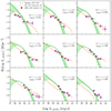 |
Fig. 2. Baseline RLF of all AGN derived from our model (green line) compared to the REX AGN RLF (purple data points) measured by Smolčić et al. (2017c). Different redshift ranges are investigated, as labeled. The boundaries of the shaded area represent the uncertainty region of the RLF as described in Sect. 2.2. In all panels we also report in orange the RL luminosity function empirically derived by Massardi et al. (2010). |
The shape of the RLF mainly depends on two parameters: the shape of the HXLF, in particular at its faint end, and the value of the dispersion σR of the L1.4 GHz−LHX relation.
Our baseline model adopts the HXLF extrapolated to low luminosities using its original slope, combined with σR = 0.5 (i.e. the 1σ scatter of the X-ray-radio relation derived by D’Amato et al. 2022). The shaded area in Fig. 2 represents the assumed uncertainties on the RLF. The lower limit of the shaded region corresponds to the RLF computed starting from the HXLF with the cut-off at log LX < 42 (Eq. (3)), and taking a slightly smaller dispersion σR = 0.4. The upper limit of the green shaded region is derived from the baseline model, but assuming a slightly larger dispersion σR = 0.65.
We note that a larger (lower) value of σR with respect to our baseline model increases (decreases) the slope of the RLF, in particular at high L1.4 GHz. The two values of the dispersion σR for the upper and lower boundaries are chosen to provide conservative estimates of the RLFs. The value σR = 0.65 is the one obtained from the D’Amato et al. (2022) sample when excluding radio upper limits; σR = 0.4 allows us to obtain a steeper slope of the RLF at high radio luminosities.
2.3. Radio number counts
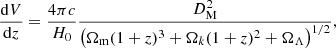
Starting from the RLF we computed the cumulative number counts (NC), namely the number of AGN above a given 1.4 GHz flux Slim and in a given redshift range in units of sr−1 or deg−2. Taking the comoving volume element:
 (9)
(9)
where DM is the comoving distance, the number of AGN per steradian with a flux S > Slim is given by:
 (10)
(10)
![Mathematical equation: $$ \begin{aligned}&\qquad \qquad =\frac{1}{4\pi } \int ^{z_{\max }}_0\int ^{L_{\max }}_{\max [l_{\lim },L_{\min }]}\Phi (L,z)\cdot \frac{\mathrm{d}V}{\mathrm{d}z} \ \mathrm{d}L \ \mathrm{d}z , \end{aligned} $$](/articles/aa/full_html/2024/07/aa48072-23/aa48072-23-eq12.gif) (11)
(11)
where llim = L1.4 GHz(Slim,z), and we fixed zmax = 10, Lmax = 1043 erg s−1 and Lmin = 1037 erg s−1.
3. Results
3.1. Luminosity function comparison
In Fig. 2 we present the RLF obtained with our model compared to that measured in the COSMOS field for REX AGN at different redshifts (Smolčić et al. 2017c).
The COSMOS REX AGN are selected as radio sources exhibiting a >3σ radio emission excess with respect to the one expected from their hosts (IR-based) SFR (Smolčić et al. 2017c). This criterion ensures that at least 80% of the radio emission in these sources is associated with an AGN, resulting in a highly reliable sample.
Figure 2 shows that our model generally predicts a higher AGN number density at low radio luminosities with respect to Smolčić et al. (2017c), while it predicts lower AGN number densities at high radio luminosities. On the other hand, the modeled RLFs are consistent with the data (within the error bars) in the intermediate luminosity range. The fact that our model cannot reproduce the high-radio luminosity AGN number densities can be explained by the fact that the assumed L1.4 GHz−LHX relation (D’Amato et al. 2022) is not valid for the RL AGN population, which is therefore not included in our model (see Sect. 2.2). To highlight the RL AGN component missed by our model, we show in Fig. 2 the empirical RL AGN luminosity function derived by Massardi et al. (2010) by summing three different populations of RL AGN: flat-spectrum radio quasars, BL Lacs and a steep spectrum RL AGN population. The three populations are described considering different evolutionary properties (see Massardi et al. 2010 for details). The RL AGN luminosity functions are in good agreement with the Smolčić et al. (2017c) datapoints at all luminosities (at least up to z ∼ 2.5), and particularly at high radio luminosities, where we expect that the REX and RL AGN classifications trace the same population.
The excess of the modeled AGN number densities at low radio luminosities can be explained as follows. AGN with low radio luminosities are more difficult to select via the statistical AGN radio-excess selection techniques since their radio emission can be easily overwhelmed by the radio emission coming from the SF of the host galaxy. Therefore, the REX AGN sample of Smolčić et al. (2017c) is probably incomplete in this low-luminosity regime. This incompleteness almost disappears when combining multiple AGN selection techniques (see Sect. 3.2).
3.2. Number counts comparison
In Fig. 3 we present the Euclidean normalized differential radio NC obtained from our model compared with other models and measurements in the literature. The green shaded area around the AGN NC, obtained using Eq. (10), reflects the assumed RLF uncertainties (see Sect. 2.2). The CTK number counts follow a trend similar to that of the total AGN population, and hence their fraction is almost constant (∼40%) with radio flux. This stems from the prescriptions of the CXB model, where ∼40% of all AGN are assumed to be CTK (once averaged over the whole luminosity range) and from the fact that radio emission is unaffected by absorption, probing the assumed intrinsic CTK AGN fraction.
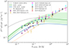 |
Fig. 3. Differential AGN number counts (NCs) derived with our model for all AGN (green line and shaded area) and CTK AGN (blue curve), compared with AGN NCs derived in the literature from different radio fields, as labeled. The uncertainties on the CTK NCs are of the same order as those of the whole AGN population but are not reported for clarity. NCs measured for the whole radio AGN population in the different works are shown as filled points, while the REX AGN only are shown as empty squares. The gray curve shows the NCs of AGN plus SFG predicted by the T-RECS simulations, while the orange curve shows the radio-loud AGN NCs derived from Massardi et al. (2010). |
It is useful to compare our AGN model with the global population of radio sources, represented by the T-RECS simulated NC (Bonaldi et al. 2019, gray line). The T-RECS simulation includes both RL AGN and SFG, dominating respectively at the highest and lowest radio fluxes. As discussed earlier on, our model does not include RL AGN. We decided not to forcibly include the RL AGN population in our model for two main reasons. First, RL AGNs are expected to constitute a small fraction of the overall AGN population, ∼10% of all the AGN, as reported by different works studying RL AGN at different redshift (Williams & Röttgering 2015; Liu et al. 2021). Second, they dominate the NC at S1.4 GHz > 0.5 − 1 mJy, as it is possible to see also from Fig. 3 (see the orange dashed line derived from the RL AGN luminosity function of Massardi et al. 2010). Therefore, they are not the main focus of this paper, where we are primarily interested in quantifying the contribution of AGN at the faintest radio fluxes. In this respect, it is worth noting that the L1.4 GHz−LHX we used for our model was derived considering an X-ray selected spectroscopically confirmed AGN+ETG sample, which is mostly composed of RQ AGN, and where no preselection based on radio excess was done (D’Amato et al. 2022). This allows us to compare our models with radio-selected samples in which AGN are not only selected based on their radio excess, but also through selection criteria based on AGN signatures at other bands (such as those discussed in Sect. 1). Thus, our model is able to account for a larger population of low-luminosity radio-selected AGN. In Fig. 3 we compare our AGN model with AGN samples extracted in some of the major deep radio surveys and fields: the 3GHz JVLA-COSMOS (Smolčić et al. 2017a,b,c), the Extended Chandra Deep Field South (ECDFS; Miller et al. 2013; Padovani et al. 2015), the Lockman-Hole (LH; Prandoni et al. 2018; Bonato et al. 2021) and the MIGHTEE radio survey (Whittam et al. 2022). The AGN NC shown in Fig. 3 as filled points are extracted from the aforementioned surveys by selecting AGN using all the available selection techniques (radio excess, X-ray emission, MIR colors, SED fitting, and spectroscopy). Instead, the squares refer to REX AGN only in the COSMOS and in the ECDFS fields. In particular, the COSMOS REX data points are derived from the same REX AGN sample that was used to build the RLF presented in Fig. 2
For fluxes S1.4 GHz < 1 mJy, the NC derived by selecting radio AGN using multiple criteria, are in a very good agreement with our AGN model predictions, down to the faintest fluxes ∼20 μJy. Instead, the data from REX AGN are below our model, with a discrepancy that increases going to fainter radio fluxes. On the contrary, the REX AGN number counts seem to be in good agreement with the RL AGN NC (orange dashed line) derived from Massardi et al. (2010). This result supports the scenario discussed in Sect. 3.1: the REX AGN RLF is incomplete, in particular at low radio luminosities (and consequently low fluxes), and it mostly accounts for the brighter RL AGN population.
As a final remark, we notice that we made some sanity checks on our AGN model. First, we compared the NC derived from our AGN model with the NC derived by the model of La Franca et al. (2010). We found that the two radio counts do not differ significantly. In particular, the NC derived in La Franca et al. (2010) predicts slightly lower AGN number densities, but still within our uncertainty region. Second, we derived the NC considering a flatter AGN radio spectral index, namely α = 0.4, finding no significant deviation from the NC derived with α = 0.7, as again they lie within our uncertainty region.
3.3. Expectations from the main radio and X-ray deep fields
We are interested in assessing the relative effectiveness of deep X-ray and radio surveys to detect the elusive obscured AGN populations and particularly CTK AGN. We use the NC derived from our radio model and the X-ray population synthesis model of the CXB, to respectively predict the number of radio-detected and X-ray detected AGN and CTK AGN over some of the major deep extragalactic radio fields, also covered by X-ray observations. We report the areas, sensitivities, and exposure times of the considered fields in Table 1. For the COSMOS field, the original 3GHz fluxes and limits were translated to 1.4 GHz assuming a spectral shape Sν ∝ ν−α, with α = 0.7.
Summary of the area covered by radio and X-ray observations, flux limits, and observing time for each of the considered fields.
Figure 4 shows the X-ray soft band (SB; 0.5–2 keV) versus 1.4 GHz flux limit plane for each of the 10 considered fields. Each field marker size is proportional to the area of the overlapping region between the observations in the two bands.
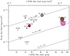 |
Fig. 4. Distribution of the 0.5 − 2 keV versus 1.4 GHz flux limit for the ten radio and X-ray fields considered in this work. The reported flux limits correspond to the faintest sources’ flux in the 0.5 − 2 keV and in the 1.4 GHz catalogs, respectively. Each field marker size is proportional to the area of the overlapping region between the radio and X-ray observations. The three dashed lines correspond to level curves for different ratios between the X-ray and radio fluxes. |
3.3.1. Number counts corrections
Our radio model forecasts the number of AGN per deg−2 with fluxes larger than a given Slim over an ideal radio field of constant sensitivity. However, in every radio pointing the sensitivity decreases from the center to its outskirt, as described by the so-called visibility function. Moreover, other issues affect the completeness of a radio catalog, such as background noise, Eddington bias (Eddington 1913), and resolution bias (Prandoni et al. 2001). The first two effects affect the incompleteness of the catalog, particularly at its faint end, while the resolution bias causes a possible loss of extended sources. To get realistic radio AGN predictions, we computed for each field a total “completeness” function (or factor) that takes into account all the aforementioned effects, and we apply it to the model forecasts. In practice we proceeded as follows. For every field we first obtained the differential NC from the sources listed in the corresponding radio catalog, namely dNcatalog/ds. These should be considered as ’raw’ NC, as no attempt to correct for the aforementioned incompleteness effects is made in this case. Then we compared dNcatalog/ds with the differential NC expected from an ideal (fully complete) catalog, namely dNideal/ds. The ratio between these two quantities defines the completeness factor:
 (12)
(12)
where  is the central flux of each flux bin. We chose the 25 deg2 mock catalog released as part of the T-RECS simulations (Bonaldi et al. 2019) as ideal catalog, as it provides a fairly good representation of the observed 1.4 GHz radio source counts, both in the bright and in the faint flux regime (Bonaldi et al. 2019; D’Amato et al. 2022). As mentioned in Sect. 3.2, the T-RECS simulations include SFG and AGN, the two main extra-galactic radio source populations detected in deep radio fields.
The completeness factors of the different fields considered in this work are presented in Fig. 5. The radio catalogs are largely incomplete at their faint end, while they are virtually complete ( ) at bright fluxes, as expected. The steep decrease of the completeness functions at faint fluxes is mainly driven by the visibility function, which represents the fraction of the survey area over which sources above a given flux density can be detected. Generally, faint sources can be detected only over a limited area, close to the center of the radio image, where the local noise is lowest, while the brightest sources can be detected everywhere, even at the outskirt of the radio images where the local noise is highest. This is reflected into a rapid decrease of the visibility function going to faint fluxes. In addition, the background noise introduces errors in the measurements of source fluxes that mostly affect the completeness at low signal-to-noise ratios and so mainly at low radio fluxes.
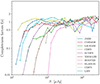 |
Fig. 5. Completeness factors of each radio catalog derived as discussed in Sect. 3.3.1. Each color represents a different radio field, as labeled. The dots represent the center of the flux bins used to compute the differential NC corrections (see text for details). |
We caveat that the correction factors shown in Fig. 5 were obtained considering both AGN and SFGs. Assuming that these corrections hold independently of the specific type of radio source considered, we can also apply them to the radio AGN-only model we built. This assumption can be justified by the fact that the faint AGN detected in deep radio fields tend to occupy the same flux density regime as SFG, and tend to be unresolved, like SFG, at the typical (arcsec-scale) angular resolution of these surveys (see e.g. Bonzini et al. 2013). This implies that SFG and AGN are similarly affected by incompleteness effects. Also Hale et al. (2023), studying the incompleteness of MIGHTEE radio images, found that the completeness corrections for the two populations are the same for a vast range of fluxes, showing only small differences for S < 10 μJy, a flux density limit not crossed by none of the considered radio catalogs. The second assumption we make is that the corrections derived in Eq. (12) hold independently of the level of AGN obscuration. Since the 1.4 GHz emission is unaffected by obscuration, this assumption appears to be fine.
3.3.2. Radio predictions
To quantify the number of AGN predicted in the different radio catalogs we applied the following equation:
 (13)
(13)
where A is the area of the radio field, Smin is the minimum radio flux density of the radio catalog and f(s) is the completeness function defined in Eq. (12). dNAGN model/ds are the differential NC derived by our model (Eq. (10)) considering 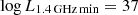 , log L1.4 GHz max = 43, zmin = 0, zmax = 10. We assigned log L1.4 GHz min = 37 since it is an acceptable threshold for the lower limit of the AGN 1.4 GHz luminosity distribution, as reported by some of the deepest radio observations performed so far (Algera et al. 2020; Alberts et al. 2020). The number of AGN and CTK AGN predicted by our model at 1.4 GHz for each field is presented on the left side of Table 2. The predictions are based on our baseline model. By using the uncertainty boundary regions described in Sect. 2.2, the prediction would get on average 30% higher (upper boundary) or 40% lower (lower boundary).
Expected number of AGN (total and CTK) compared with the total number of sources observed in each field.
The top panel of Fig. 6 shows the fraction of AGN and CTK AGN expected by our model obtained by dividing the predicted number of AGN by the whole number of radio sources in each radio catalog. The fields are sorted in ascending order of radio flux limit. The expected fraction of AGN ranges between 36% in the J1030 field, the deepest radio field in our sample, up to 53% in the BOOTES and ELAIS-S1 fields, which are among the shallowest ones. The top panel of Fig. 6 shows a clear trend where the AGN fraction in radio catalogs decreases as the sensitivity of the survey increases. This is in accordance with the evidence, presented by several works in literature and also shown in Fig. 3, that AGN dominates over SFGs in the bright-fluxes regime of the global radio NCs (gray line in Fig. 3). On the contrary, the lower the radio flux, the larger the relative contribution of SFG to the global radio NC (see again Fig. 3), and consequently also the fraction of AGN gets reduced.
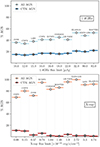 |
Fig. 6. Upper panel: predicted fractions of AGN (light blue) and CTK AGN (dark blue) as a function of radio survey flux limit. Lower panel: same as in the upper panel but for the X-ray predictions. In both panels the surveys are sorted on the x-axis by increasing flux limit (faintest source in the catalog). |
All our predictions, particularly those for the shallower fields, have to be considered conservative. Indeed, the given AGN fractions do not include, by construction, the most powerful radio AGN (the RL population) that dominate the bright end of the NC. About ∼40% of all AGN, that is about ∼20% of the radio sources in each catalog, are expected to be CTK nuclei, as reported also in Sect. 3.2.
3.3.3. X-ray predictions
To compare radio versus X-ray AGN yields in the considered fields, we proceeded as follows. We computed the AGN differential number counts based on the CXB model, taking log LX min = 41, log LX max = 47, zmin = 0, zmax = 10. The X-ray lower limit log LX min = 41 corresponds to the radio lower limit log L1.4 GHz min = 37 used in Eq. (13), when assuming the L1.4 GHz−LHX relation of our model. This value is also a reasonable lower limit to the known AGN X-ray luminosity distribution, and we checked that this choice does not violate the total CXB flux constraint. Using the sky coverage A(s) and the CXB differential NC, dNAGN CXB/ds, the number of AGN over a certain X-ray field is predicted as follows:
 (14)
(14)
where Smin is the minimum SB X-ray flux of the respective catalog and A(s) represents the sky coverage, namely the observed area as a function of the sensitivity of the survey. The function A(s) is generally retrieved by performing completeness simulations, already implementing any possible completeness correction factor. The results are reported on the right side of Table 2.
We show only the predictions in the SB for two reasons. Firstly, the numbers of AGN and CTK AGN predicted by the CXB model in the SB are larger than in the hard band (HB, 2 − 10 keV), for every field. Indeed, for all the considered fields, the flux limit in the SB is always lower by a factor ∼5 − 10 than the one in the HB, according to the fact that for all the X-ray catalogs the number of sources detected in the SB is larger than in the HB2. Secondly, the expected fraction of CTK AGN predicted by the CXB model is larger in the SB than in the HB for z > 0. This happens because of the deeper SB flux limit and because of the presence of a minor (but not negligible) SB reflected component in the CTK AGN rest-frame spectrum implemented in the CXB model (Fig. 1 in Gilli et al. 2007). We finally notice that in the case of the XMM-LSS field, the number of AGN predicted by the X-ray model exceeds the number of X-ray sources in the related catalog by a fraction ∼15%. This excess can be justified by field-to-field variation of the number counts or by an overestimate of the CXB model in the SB already observed in a previous work (Marchesi et al. 2020).
In the lower panel of Fig. 6 we report the fraction of X-ray AGN and CTK AGN predicted over the different X-ray fields sorted by increasing X-ray flux limit. In the X-ray band AGN are the dominant population: in all cases the fraction of AGN is ≥70%, with again an increasing trend for shallower flux limits. Indeed, the X-ray emission of SFGs starts to be detected only at very faint fluxes, and are rarely detected in the shallower surveys. The increasing trend of the AGN fraction going to higher flux limits in the X-ray panel is more scattered than in the radio panel. This is mainly due to the shapes of the sky coverage of the different X-ray observations that can change significantly from field to field. In general, X-ray surveys allow the detection of a larger fraction of AGN with respect to radio ones, where the contamination from SFG can be large, especially at faint fluxes. However, the large majority of the AGN detected in the X-rays are not heavily obscured: the fraction of CTK AGN in the X-rays is always between 1%–11% of all the X-ray sources and between the 1%–15% of all the X-ray AGN predicted by the CXB model, the larger fraction reached in the deepest survey, namely the CDFS. Indeed, the fraction of detectable CTK AGN shows a remarkable dependence on the X-ray flux limit: the lower the X-ray flux limit the higher the fraction of CTK AGN detected. This trend is justified by the fact that heavily obscured sources are usually very faint in the X-rays and so their detection requires very deep surveys. On the contrary, in the radio band, the CTK AGN are between 14 − 22% of all the radio sources and ∼40% of all the radio AGN predicted by our model, and show an opposite dependence on radio flux limit.
3.4. AGN densities
In Fig. 7 we plot the radio and X-ray densities predicted by the two models for both total and CTK AGN. These densities, also reported in Table 2, are computed by dividing the number of AGN predicted by the area of the radio or X-ray observations. In the upper panel, we note that the X-ray observations generally return a larger density of AGN per arcmin−2, except for the J1030, LHN and COSMOS fields. However, the differences between the densities predicted in the two bands are generally less than one order of magnitude. When only the CTK population is taken into account (lower panel) the situation is the opposite: for every field (except the CDFS) the CTK AGN density is much larger in the radio than in the X-rays, by even more than one order of magnitude. Furthermore, as one would expect, the 1.4 GHz AGN and CTK AGN densities increase for deeper radio observations.
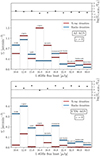 |
Fig. 7. Upper panel: AGN densities in X-ray (red) and radio (blue) surveys as a function of 1.4 GHz survey flux limit, as reported in Table 2. The ratio between the 1.4 GHz and X-ray AGN densities is shown in the top position of the plot. Lower panel: same as in the upper panel but for CTK AGN. In both panels the surveys are sorted on the x-axis by increasing radio flux limit (faintest source in the catalog). |
These two plots clearly show that X-ray observations are on average more effective than radio ones in detecting AGN when the global AGN population is considered, but if we want to detect the most obscured AGN the radio selection is more effective than the X-ray one (by on average a factor of 10 in term of surface densities). In Sect. 4.3 we show that this result holds even at high redshift.
4. Discussion
4.1. Radio catalogs: AGN predictions versus observations
Since the radio model we built is not set to predict only the REX AGN population but, as presented in Sect. 3.2, it can be used to forecast the whole population of radio-quiet AGN we compared our results with those found in the literature using multiple selection techniques.
In the case of the COSMOS field, as mentioned in Sect. 3.1, Smolčić et al. (2017a) distinguished radio sources into pure SFG, medium-luminosity AGN (MLAGN), and high-luminosity AGN (HLAGN). Using color selection, X-ray counterpart analysis, SED fitting decomposition, and radio excess, they identified 1623 HLAGN and 1648 MLAGN among all the radio sources with a counterpart in the COSMOS2015 photometric catalog (Laigle et al. 2016). All the AGNs represent around the 42% of the COSMOS radio sources in the reference catalog, a fraction very close to the 45% of AGN our model predicts for COSMOS. However, our predictions have to be considered conservative since our model does not take into account the classical RL AGN, which are expected to be around 10% of the whole AGN population. In the same work, Smolčić et al. (2017a) made also an AGN selection based only on the radio information, selecting only those AGN showing a (> 3σ) radio excess with respect to what is expected from a pure SFG, to ensure that at least the 80% of their radio emission is due to the AGN component. Their final REX AGN sample is constituted by 1846 sources, that is only 26% of all the radio sources in COSMOS. This shows that the radio excess technique alone is not able to provide complete AGN samples, and multiple selection methods are needed to this end.
Recent MIGHTEE observations of the COSMOS field (Whittam et al. 2022; Zhu et al. 2023) obtained results similar to those of Smolčić et al. (2017a). The 1.4 GHz MIGHTEE data in the COSMOS field reach almost the same sensitivity as the 3GHz VLA COSMOS image, but was obtained on a smaller portion of the field ∼ 1.6 deg2. Using the radio excess criterion, following the more recent prescriptions of Delvecchio et al. (2021), Whittam et al. (2022) found 1332 radio excess AGN over a sample of 5223 sources, corresponding to ∼25%. On the contrary, when they account for all the other selection techniques, they retrieve a fraction of AGN around 35%. Whittam et al. (2022) also present a consistent fraction of unclassified sources; if these are split into AGN and SFG based on the flux density ratio of the classified sources, the fraction of the whole AGN gets to ∼40%, close to our predictions.
Another example comes from the radio observation of the CDFS (Miller et al. 2013), where source classification is reported in Bonzini et al. (2013) and Padovani et al. (2015). Among the 883 radio sources in their catalog, they identified 381 AGN (43%) using IRAC colors, X-ray counterparts, and the radio excess parameter. Our model predicts a similar number of AGN (361) that has to be taken as a conservative estimation since RL AGN are excluded. Bonzini et al. (2013) selected as REX AGN only 173 sources, only 19% of the whole radio sources, again suggesting that when multiple, deep, multiband analyses are adopted the completeness of the radio AGN sample largely increases and the number of AGN get very similar to what is predicted by our model.
The radio selection of heavily obscured AGN has been only marginally investigated in the literature. The works mentioned above did not investigate the radio properties of AGN in terms of their obscuration levels. Instead Andonie et al. (2022), starting from an IR-based AGN selection in the COSMOS field (and limiting to z < 3), investigated the obscuration properties of their sample by means of X-ray and radio data. They found that 73% of IR-selected AGN were in the VLA 1.4 GHz or 3GHz catalogs, and in particular that 63% of these radio detected AGN are obscured (log NH > 22).
Despite the broad agreement with the total number of AGN observed in radio catalogs, we remark that the number of heavily obscured CTK AGN expected by our model is driven by the assumptions made in the CXB modeling, and is therefore affected by the uncertainties discussed below. The population synthesis model of the CXB considers X-ray data that extend beyond the traditional 0.5–10 keV band (the peak of the CXB is around 20-30keV), allowing one to constrain the population of heavily obscured AGN better than what is possible with Chandra and XMM-Newton observations alone. However, the derived total abundance of CTK AGN, and in particular that of the most heavily obscured, reflection-dominated AGN (log NH > 25), is degenerate with the reflection efficiency, and hence overall normalization, assumed for their X-ray spectra. In principle, by decreasing the reflection efficiency by a factor of ∼2, which would still be consistent with broad band X-ray observations of local CTK AGN, would increase the number of reflection-dominated CTK AGN by an equal factor. An additional uncertainty is related to the scatter of the measured CXB intensities. For example, Comastri et al. (2015) showed that by assuming a space density of reflection-dominated CTK AGN 4x larger than what was assumed by Gilli et al. (2007), the produced CXB flux would still be in agreement with the CXB measurements within their scatter. However, we do not expect the fraction of CTK AGN to be severely higher (or lower) than what we assumed, as suggested by number of works in the literature that searched for CTK AGN by means of multiband tracers that are in principle not affected by obscuration and can be used as proxies of the intrinsic AGN nuclear power. For example, Daddi et al. (2007) and Fiore et al. (2009) selected CTK AGN by means of their mid-IR excess (hot dust) emission as compared to their X-ray emission, finding space densities of CTK AGN at z ∼ 1.5 − 2.0 consistent with the CXB model expectations. A similar agreement was found at z ∼ 0.8 by Vignali et al. (2014) who selected obscured AGN through their narrow [Ne v]3426 Å emission line. The uncertainties related to the high-redshift predictions of our model will be discussed in Sect. 4.3.
4.2. Radio versus X-ray AGN detection
For a given combination of radio and X-ray flux limits the relative efficiency of the two bands in detecting an AGN depends on the shape of the AGN spectral energy distribution, which in turn depends on a number of physical properties like the SMBH’s accretion parameters, the presence of radio jets, the duty cycle, the bolometric luminosity and the obscuration level.
Here we want to investigate the detection efficiency of 1.4 GHz and X-ray selections by varying three main AGN parameters: redshift, bolometric luminosity and obscuration level. Starting from a fixed bolometric luminosity, we computed the HB X-ray AGN luminosity using the bolometric correction derived in Duras et al. (2020), which are valid both for type 1 and type 2 AGN. Then we converted the HB X-ray luminosity into the corresponding SB luminosity assuming a power-law spectrum with photon index Γ = 1.9 (Piconcelli et al. 2005; Gilli et al. 2007). To derive the X-ray flux we used one of the X-ray source mock catalogs presented in Marchesi et al. (2020). The considered catalog contains 5.4M sources simulated down to very faint X-ray fluxes, 10−20 erg cm−2 s−1, over an area of 100 deg2 and with different obscuring hydrogen column densities, following the prescription of the CXB model in G07. The catalog provides the SB flux and the corresponding SB X-ray luminosity for each source at a given redshift and obscuration level. Therefore, from given combination of SB X-ray luminosity and obscuration, we derived X-ray flux versus redshift dependences.
The intrinsic X-ray luminosity was then converted into 1.4 GHz luminosity using Eq. (5). Finally, by considering the 1.4 GHz luminosity-flux relation:
 (15)
(15)
we obtain the corresponding radio flux density (S1.4 GHz). In Fig. 8 we report the AGN X-ray versus radio flux density for redshifts between z = 0 and z = 9, considering two different bolometric luminosities and three different levels of AGN obscuration. We also report as error bars the 1σ intervals produced by the scatter in the Lbol − LHX relation (σ = 0.27 dex, vertical direction), and in the L1.4 GHz−LHX relation (σ = 0.5 dex, horizontal direction).
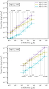 |
Fig. 8. Typical SB X-ray flux versus 1.4 GHz flux at different redshifts computed for an AGN with log Lbol = 43 (upper panel) and log Lbol = 46 (lower panel). Error bars show the 1σ distribution values due to the scatter in the Lbol − LHX relation (vertical error bar), and in the L1.4 GHz−LHX relation (horizontal error bar). The dashed lines indicate the redshift at which the fluxes are computed. |
At any given redshift, the 1.4 GHz AGN flux density is the same for the three levels of AGN obscuration, since the radio emission is not affected by obscuration. On the contrary, the X-ray fluxes at the same redshift differ significantly and decrease with increasing obscuration. We notice that the X-ray flux of an obscured AGN (log NH = 22.5) at a given bolometric luminosity tends to approximate the flux of unobscured AGN (log NH = 20.5) for z > 3. This is due to the effect of the K-correction that shifts absorption out of the X-ray bandpass for AGN at high-z. Considering the two values of log Lbol the trend of the AGN fluxes are similar for corresponding values of NH, but with a shift of ∼2 orders of magnitude in radio and of 2.5 dex in the X-ray.
To understand which AGN are detectable in the radio and/or X-ray fields considered in this work, we compared these curves with the fields’ X-ray and radio median sensitivities. In each panel of Fig. 9 we plot the 1.4 GHz median flux limit (5σmed) versus the X-ray sensitivity at 50% of the field area (that can be seen as a median X-ray flux limit). These are compared with the tracks showing X-ray versus radio fluxes for AGN at two given obscuration levels and two different bolometric luminosities.
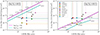 |
Fig. 9. Median SB X-ray and 1.4 GHz detection fluxes for each of the fields color-coded as labeled in the right panel. The two panels consider tracks for two different levels of AGN obscuration: log NH = 20.5 (left) and log NH = 24.5 (right). In cyan and in magenta we show the typical 0.5 − 2 keV versus 1.4 GHz flux tracks, computed at different redshifts, for an AGN with log Lbol = 43 and log Lbol = 46, respectively. |
As shown in Fig. 9, the tracks for unobscured AGN (log NH = 20.5; left panel), intercept the vertical projection of all the fields’ positions before intersecting the horizontal ones. This means that, when typical unobscured AGN reaches the median radio sensitivity of the fields, its X-ray flux is largely above the median X-ray sensitivity of the same fields. Therefore, when an unobscured AGN is detected in the radio band, it is already detected also in the X-ray image of the same field. This justifies why, as we see in Sect. 3.3.3, unobscured AGN are preferentially detected in the X-rays for all the considered fields.
A very different behavior is observed for CTK AGN, with log NH = 24.5 (right panel). In this case, for most of the fields, the AGN tracks intercept the horizontal projections before the vertical ones, meaning that when one of these AGN becomes detectable in the X-ray it is already detected in the radio image of the field. The only field for which this is not true for both values of log Lbol is the 7Ms CDFS, where, due to the deep Chandra imaging, X-ray selection is more effective than radio selection in identifying AGN even in the presence of heavy obscuration. In the 2Ms CDFN, the detection efficiency of luminous (log Lbol = 46) CTK AGN is the same for both radio and X-ray observations: the tracks in Fig. 9 (right) exactly crosses the CDFN datapoints. Less luminous CTK AGN are instead preferentially detected in the radio band.
4.3. High redshift predictions
In Table 3 we report the predictions of our model for AGN and CTK AGN at z > 3. For consistency with the assumptions in our baseline model for radio AGN, we use for the X-rays the expectations of Vito et al. (2014) as implemented in the corresponding mock catalog (see Marchesi et al. 2020). The procedure followed to forecast the number of detectable high-z AGN is the same as reported in Sects. 3.3.2 and 3.3.3.
Expected number and surface densities of z > 3 AGN (total and CTK) in each field both in the radio (left) and X-ray band (right).
The change in the starting HXLF also allows us to introduce an intrinsic increment in the fraction of heavily obscured AGN at z > 3, that has been observed or predicted by different works in the literature (Aird et al. 2015; Ananna et al. 2019; Gilli et al. 2022b; Ni et al. 2020; Lapi et al. 2020).
In the CXB model the fraction of CTK AGN depends on the luminosity and reaches 4/9 only for the low luminosity regime or, equivalently, at the faintest X-ray fluxes (see Eq. (4) in Gilli et al. 2007). On the contrary, in Vito et al. (2014) HXLF, we assumed (according to Vito et al. 2018; Marchesi et al. 2020) a luminosity-independent and constant fraction of CTK AGN equal to 4/9 of the whole AGN population.
The number of X-ray AGN reported in Table 3 are obtained considering the 0.5−2 keV X-ray band, for which the total number of AGN detected at z > 3 is larger than in the HB. We verified that using the HB, we would have obtained larger numbers of CTK AGN (within a factor of 2), but we kept the SB information for consistency with the previous sections.
In Fig. 10 we show the densities of AGN (upper panel) and CTK AGN (lower panel) both in the radio and X-ray band. The densities of z > 3 AGN are, for both the bands, ∼1.5 dex lower than what was predicted for z > 0, remarking the difficulty of detecting such high-redshift sources with surveys with the current facilities. Even at z > 3, X-ray observations are more efficient in detecting unobscured or mildly obscured AGN (predicting AGN surface densities on average 10 times larger than the radio ones), whereas the radio model predicts much larger CTK AGN densities for all the fields (except the CDFS). At z > 3 the surface density of CTK AGN radio detected is generally more than 10 times larger than the X-ray one and more than 100 times larger for half of the fields. This strongly supports the radio selection’s effectiveness in detecting heavily obscured AGN, even at high redshift.
4.4. SKA predictions
By the end of this decade, the Square Kilometer Array Observatory (SKAO) will become fully operational. As reported in Prandoni & Seymour (2015), SKAO will have among its primary science drivers the investigation of the SMBH-galaxy coevolution and the astrophysics related to the accretion processes. Prandoni & Seymour (2015) have proposed three 1.4 GHz radio continuum surveys, optimized to address AGN and galaxy evolution science cases. These surveys are organized in tiers, following a nested wedding cake strategy; the Ultra-Deep, the Deep, and the Wide surveys with the following area – 1σ sensitivity combinations: 0.05 μJy over 1 deg2, 0.2 μJy over 10–30 deg2, 1 μJy over 103 deg2, respectively.
Using the NC derived from our 1.4 GHz model we computed the number of AGN and CTK AGN detectable in the three different survey tiers for high-redshift (z > 3) and very high-redshift (z > 6, z > 10) ranges. The results for the three tiers are reported in Table 4. All the predictions are computed assuming a flat sensitivity over the survey area. With the wide SKA survey thousands of AGN are expected to be detected at z > 6 and a consistent fraction of them is expected to be CTK (at least > 45%). Also for z > 10, a redshift range that since the advent of JWST was almost completely unexplored, SKA will be able to detect several tens of AGN.
Expected number of high-z AGN in the three 1.4 GHz continuum surveys planned with SKAO.
The z > 6 universe is still very unconstrained, particularly for the AGN X-ray and radio LFs. Without better information, we decided to use our baseline radio model and to extrapolate it to higher redshifts. However, we are aware that the results should be taken cautiously. For example, we assumed that the radio-to-X-ray relation measured by D’Amato et al. (2022) holds even at z ≫ 3, but we did not consider whether the increased ISM density at high-z (Gilli et al. 2022b) may provide stronger free-free absorption and depress radio emission. Similarly, we did not consider whether the effects of self-synchro absorption (SSA) may depress radio emission as well, as one would require on average stronger magnetic fields to overcome energy losses by Comptonization of the enhanced CMB photon field. We defer a detailed discussion of these effects to future work entirely dedicated to SKA forecasts. Another uncertain aspect is the fraction of CTK AGN at these redshifts. While our z > 3 baseline model assumes a constant fraction of CTK AGN, the large majority of the AGN above z > 6 are expected to be CTK (Gilli et al. 2022b; Ni et al. 2020; Lapi et al. 2020; Lambrides et al. 2020; Lusso et al. 2023).
At z = 6 the 5σ sensitivities of the three survey correspond to 1.4 GHz luminosities of 7.8 × 1037 erg s−1, 3.1 × 1039 erg s−1, 1.5 × 1040 erg s−1 respectively for the Ultra-Deep, Deep and Wide surveys. Converting the 1.4 GHz luminosity into the corresponding HB X-ray intrinsic luminosity using Eq. (5), and taking the HX to bolometric luminosity correction factor of Duras et al. (2020), we derived the minimum z > 6 AGN bolometric luminosity that SKA would detect in each of the three surveys. These bolometric luminosity lower limits corresponds to Lbol ∼ 2 × 1044 erg s−1 for the Ultra-Deep, Lbol ∼ 1045 erg s−1 for the Deep and Lbol ∼ 8 × 1045 erg s−1 for the Wide survey.
To investigate the population of AGN that SKA will detect in the three surveys, we used the X-ray AGN mock catalog generated using the Vito et al. (2014) HXLF and provided in Marchesi et al. (2020). This 100 deg2 catalog includes ∼2.5 × 10⁶ AGN in the redshift range 3 < z < 20 down to a 0.5–2 keV luminsoity log LSB = 40, reaching fluxes below ∼ 2 × 10⁻²⁰ erg s−1 cm−2. Using the same relations as in Sect. 4.2, we derived the bolometric luminosity, the 1.4 GHz luminosity and the flux density of each source.
The panels of Fig. 11 show the distribution in log L1.4 GHz and log Lbol of the z > 6 sources with a radio flux density larger than the sensitivity threshold of the three tiers.
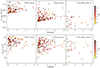 |
Fig. 11. Simulated z > 6 AGN to be detected by SKAO in the three tiers of its continuum 1.4 GHz surveys. Each point is color-coded according to its obscuration level. The top three panels show the distribution of log L1.4 GHz while the bottom panels show the distribution of log Lbol. The number of simulated sources in the Wide survey panels is almost 1/10 of the number of AGN reported in Table 4 (see text for details). |
Since the area of the mock catalog is 1/10 of the area of the Wide SKA survey, the number of sources in the Wide Survey panel is almost 1/10 of the AGN predicted for the respective survey at z > 6 and reported in Table 3. The median bolometric luminosities of AGN detected in the three surveys, at z > 3, z > 6, and z > 10 are reported in Table 4.
We remind that the L1.4 GHz−LHX relation used to derive the radio luminosities from the mock X-ray catalog does not include the most powerful RL AGN that should populate a fainter region of the log Lbol distribution. Furthermore, the upper limits of the distributions of the bolometric and radio luminosities presented in Fig. 11 are affected by the shape of the HXLF of Vito et al. (2014). These HXLF are partially incomplete in their brightest part, since they were computed on deep pencil-beam X-ray fields that miss the most luminous X-ray sources. Taking into account a larger fraction of bright X-ray sources the log Lbol distribution in Fig. 11 would extend to larger values.
The possibility to identify thousands of AGN and CTK AGN at z > 6 will transform our understanding of the co-evolution of MBHs with their galaxies in the first Gyr of the cosmic time.
The combination of radio data from SKA with multiband data from current and next-generation facilities will be crucial to detect distant AGN and separate them from SFGs. Indeed SKA surveys are planned to overlap with forthcoming wide-area, sensitive optical and NIR-surveys, like those by LSST and Euclid (see Prandoni & Seymour 2015 for a detailed list of the multiwavelength survey synergies). Therefore, it will be possible to apply radio-excess (REX) selection techniques similar to those mentioned earlier in this work (see e.g. Smolčić et al. 2017c) to very large statistical samples, and especially at high redshifts. In addition, in combination with ALMA follow-up data, SKA will prove whether the far-infrared-radio correlation normally used to separate AGN and SFGs is still valid at high-z, and also for low stellar masses and SFR. As an example, the sensitivity of the SKA deep surveys will allow detection of SFR ∼ 10 M⊙ yr−1 in galaxies up to z ∼ 3 − 4, and SFR ≥ 50 M⊙ yr−1 at z ∼ 6 − 7 (McAlpine et al. 2015). Observations of well-known extra-galactic fields where dense multiband information, from UV to far-IR, is available will in particular increase the identification efficiency of CTK AGN. JWST and ELT observations will also allow for spectroscopic follow-up of radio-selected, high-z AGN candidates to determine their redshift and ultimately measure the radio AGN luminosity function at z > 6. The combination of the SKA radio observations with future X-ray data from telescopes like STAR-X3, Athena (Nandra et al. 2013), and AXIS (Mushotzky et al. 2019) will enable improved AGN identification and measurement of ther column densities.
In the absence of other multiband AGN diagnostics, the identification of AGN and CTK AGN using SKA data may rely on either multifrequency radio information, or high-resolution (SKA 10GHz observations will provide angular resolution of 0.05″ − 0.1″ compared to the 0.4″ − 0.5″ of 1.4 GHz observations) and/or multi-epoch follow-ups. All these diagnostics are amply used in the literature. Flat or convex radio spectral indices would point to the presence of compact AGN cores (O’Dea & Saikia 2021). High-resolution follow-ups can pinpoint AGN through the measurement of high (T > 105 − 6 K) brightness temperatures (see Morabito et al. 2022), while multi-epoch observations may identify the tiny fraction of variable AGN at μJy flux density levels (Radcliffe et al. 2019).
5. Conclusions
In this work we developed an analytical model to compute the 1.4 GHz luminosity function and associated number counts for the whole AGN population and for subpopulations of AGN with different obscuration levels. In particular, we converted into the radio band the prescriptions of the population synthesis model of the CXB using an X-ray to radio luminosity relation derived for faint X-ray sources.
We applied our model to some of the major extragalactic fields covered by deep radio and X-ray observations to predict the number of AGN and CTK AGN detectable in each band.
The main results can be summarized as follows:
-
We found a very good agreement between the number of radio-detected AGN predicted by our model in the fields and the observed number of AGN identified via multiple selection techniques. This means that our model is able to give an almost complete census of the radio AGN population, excluding the minority population of RL AGN, that is missed by construction.
-
On average X-rays are able to detect a larger number of AGN, but most of the X-ray detected AGN are unobscured. The CTK AGN surface density detected at 1.4 GHz is on average 10 times higher than the X-ray one. This result stands also at high redshift (z > 3), where the surface density of CTK AGN expected in radio surveys becomes, for some fields, even 103 times larger than the X-ray density.
-
Our model predicts the existence of thousands of CTK AGN already detected in the radio fields investigated in this work that are largely missed by the corresponding X-ray observations. Both our model and the results coming from the literature suggest that radio emission may provide an unbiased picture (in terms of obscuration) of the AGN demography. However, multiple selection techniques employing different multiwavelength indicators of nuclear activity are required to identify AGN among SFGs. The investigation of the CTK AGN selection among the sources in the available radio catalogs will be the focus of the next-coming work.
-
In the future the SKAO will be able to detect in its three-tier surveys more than 2000 AGN at z > 6 (down to log Lbol ∼ 43) and some tens at z > 10, opening new windows in exploration of the AGN parameter space at these redshifts.
In this work we demonstrated that radio emission can be a powerfull tool to detect the elusive population of heavily obscured, Compton-thick AGN. In the future, the synergies between deep continuum surveys performed by SKA and multiband information provided by present and future telescopes and observatiories, will allow for an extensive testing of radio-based AGN selection tecniques on large statistical samples, and for a detailed exploration of the radio emission properties of these objects in the high-z Universe.
REX AGN are a distinct class with respect to RL AGN, as in the former the observed radio emission is compared to the infrared emission due to star formation, while in the latter the radio emission is compared to the AGN-related emission observed for instance at optical or X-ray bands (see Kellermann et al. 1989; Terashima & Wilson 2003). Nevertheless, RL AGN are also REX AGN as they also satisfy the REX definition.
The only exception is the J1030 field, where the number of X-ray sources reported in Nanni et al. (2020) in the SB (HB) is 193 (208). However, the Chandra observation of the J1030 filed is the latest one among those considered in this work and suffers from the SB Chandra sensitivity deterioration (Peca et al. 2021).
Acknowledgments
K.I. acknowledges the support under the grant PID2022-136827NB-C44 provided by MCIN/AEI/10.13039/ 501100011033/FEDER, EU. We thank the anonymous referee for useful suggestions which improved the quality of the paper. We acknowledge financial support from the grant PRIN MIUR 2017PH3WAT (‘Black hole winds and the baryon life cycle of galaxies’). IP and RG acknowledge support from INAF under the Large Grant 2022 funding scheme (project “MeerKAT and LOFAR Team up: a Unique Radio Window on Galaxy/AGN co-Evolution”). We acknowledge useful discussion with I. Delvecchio, T. Costa, F. La Franca.
References
- Aird, J., Coil, A. L., Georgakakis, A., et al. 2015, MNRAS, 451, 1892 [Google Scholar]
- Alberts, S., Rujopakarn, W., Rieke, G. H., Jagannathan, P., & Nyland, K. 2020, ApJ, 901, 168 [NASA ADS] [CrossRef] [Google Scholar]
- Algera, H. S. B., van der Vlugt, D., Hodge, J. A., et al. 2020, ApJ, 903, 139 [Google Scholar]
- Ananna, T. T., Treister, E., Urry, C. M., et al. 2019, ApJ, 871, 240 [Google Scholar]
- Andonie, C., Alexander, D. M., Rosario, D., et al. 2022, MNRAS, 517, 2577 [NASA ADS] [CrossRef] [Google Scholar]
- Aravena, M., Boogaard, L., Gónzalez-López, J., et al. 2020, ApJ, 901, 79 [NASA ADS] [CrossRef] [Google Scholar]
- Assef, R. J., Stern, D., Kochanek, C. S., et al. 2013, ApJ, 772, 26 [Google Scholar]
- Ballantyne, D. R. 2009, ApJ, 698, 1033 [NASA ADS] [CrossRef] [Google Scholar]
- Barchiesi, L., Pozzi, F., Vignali, C., et al. 2021, PASA, 38, e033a [NASA ADS] [CrossRef] [Google Scholar]
- Becker, R. H., White, R. L., & Helfand, D. J. 1995, ApJ, 450, 559 [Google Scholar]
- Becker, R. H., White, R. L., Gregg, M. D., et al. 2001, ApJS, 135, 227 [NASA ADS] [CrossRef] [Google Scholar]
- Biggs, A. D., & Ivison, R. J. 2006, MNRAS, 371, 963 [Google Scholar]
- Blandford, R. D., & Znajek, R. L. 1977, MNRAS, 179, 433 [NASA ADS] [CrossRef] [Google Scholar]
- Bonaldi, A., Bonato, M., Galluzzi, V., et al. 2019, MNRAS, 482, 2 [Google Scholar]
- Bonato, M., Prandoni, I., De Zotti, G., et al. 2021, MNRAS, 500, 22 [Google Scholar]
- Bonzini, M., Padovani, P., Mainieri, V., et al. 2013, MNRAS, 436, 3759 [Google Scholar]
- Boquien, M., Burgarella, D., Roehlly, Y., et al. 2019, A&A, 622, A103 [NASA ADS] [CrossRef] [EDP Sciences] [Google Scholar]
- Brammer, G. B., van Dokkum, P. G., & Coppi, P. 2008, ApJ, 686, 1503 [Google Scholar]
- Brunner, H., Cappelluti, N., Hasinger, G., et al. 2008, A&A, 479, 283 [NASA ADS] [CrossRef] [EDP Sciences] [Google Scholar]
- Brusa, M., Fiore, F., Santini, P., et al. 2009, A&A, 507, 1277 [NASA ADS] [CrossRef] [EDP Sciences] [Google Scholar]
- Buchner, J., Georgakakis, A., Nandra, K., et al. 2015, ApJ, 802, 89 [Google Scholar]
- Chen, C. T. J., Brandt, W. N., Luo, B., et al. 2018, MNRAS, 478, 2132 [NASA ADS] [CrossRef] [Google Scholar]
- Civano, F., Marchesi, S., Comastri, A., et al. 2016, ApJ, 819, 62 [Google Scholar]
- Comastri, A., Gilli, R., Marconi, A., Risaliti, G., & Salvati, M. 2015, A&A, 574, L10 [NASA ADS] [CrossRef] [EDP Sciences] [Google Scholar]
- Daddi, E., Alexander, D. M., Dickinson, M., et al. 2007, ApJ, 670, 173 [NASA ADS] [CrossRef] [Google Scholar]
- D’Amato, Q., Prandoni, I., Gilli, R., et al. 2022, A&A, 668, A133 [NASA ADS] [CrossRef] [EDP Sciences] [Google Scholar]
- Decarli, R., Pensabene, A., Diaz-Santos, T., et al. 2023, A&A, 673, A157 [NASA ADS] [CrossRef] [EDP Sciences] [Google Scholar]
- Delhaize, J., Smolčić, V., Delvecchio, I., et al. 2017, A&A, 602, A4 [NASA ADS] [CrossRef] [EDP Sciences] [Google Scholar]
- Delvecchio, I., Smolčić, V., Zamorani, G., et al. 2017, A&A, 602, A3 [NASA ADS] [CrossRef] [EDP Sciences] [Google Scholar]
- Delvecchio, I., Daddi, E., Sargent, M. T., et al. 2021, A&A, 647, A123 [NASA ADS] [CrossRef] [EDP Sciences] [Google Scholar]
- de Vries, W. H., Morganti, R., Röttgering, H. J. A., et al. 2002, AJ, 123, 1784 [Google Scholar]
- Dong, A.-J., Ge, K., Liu, X., & Zhi, Q.-J. 2021, Astron. Nachr., 342, 191 [NASA ADS] [CrossRef] [Google Scholar]
- Donley, J. L., Koekemoer, A. M., Brusa, M., et al. 2012, ApJ, 748, 142 [Google Scholar]
- Duras, F., Bongiorno, A., Ricci, F., et al. 2020, A&A, 636, A73 [NASA ADS] [CrossRef] [EDP Sciences] [Google Scholar]
- Eddington, A. S. 1913, MNRAS, 73, 359 [Google Scholar]
- Fan, X.-L., & Bai, J.-M. 2016, ApJ, 818, 185 [NASA ADS] [CrossRef] [Google Scholar]
- Fiore, F., Puccetti, S., Brusa, M., et al. 2009, ApJ, 693, 447 [NASA ADS] [CrossRef] [Google Scholar]
- Franzen, T. M. O., Banfield, J. K., Hales, C. A., et al. 2015, MNRAS, 453, 4020 [Google Scholar]
- Gilli, R., Comastri, A., & Hasinger, G. 2007, A&A, 463, 79 [NASA ADS] [CrossRef] [EDP Sciences] [Google Scholar]
- Gilli, R., Ghigo, M., Marchesi, S., et al. 2022a, Mem. Soc. Astron. Ital., 93, 236 [NASA ADS] [Google Scholar]
- Gilli, R., Norman, C., Calura, F., et al. 2022b, A&A, 666, A17 [NASA ADS] [CrossRef] [EDP Sciences] [Google Scholar]
- Greene, J. E., Labbe, I., Goulding, A. D., et al. 2024, ApJ, 964, 39 [CrossRef] [Google Scholar]
- Hale, C. L., Whittam, I. H., Jarvis, M. J., et al. 2023, MNRAS, 520, 2668 [NASA ADS] [CrossRef] [Google Scholar]
- Hasinger, G., Miyaji, T., & Schmidt, M. 2005, A&A, 441, 417 [NASA ADS] [CrossRef] [EDP Sciences] [Google Scholar]
- Heywood, I., Hale, C. L., Jarvis, M. J., et al. 2020, MNRAS, 496, 3469 [NASA ADS] [CrossRef] [Google Scholar]
- Hickox, R. C., & Alexander, D. M. 2018, ARA&A, 56, 625 [Google Scholar]
- Hildebrand, R. H. 1983, QJRAS, 24, 267 [NASA ADS] [Google Scholar]
- Hopkins, P. F., Hernquist, L., Cox, T. J., & Kereš, D. 2008, ApJS, 175, 356 [Google Scholar]
- Kellermann, K. I., Sramek, R., Schmidt, M., Shaffer, D. B., & Green, R. 1989, AJ, 98, 1195 [Google Scholar]
- La Franca, F., Melini, G., & Fiore, F. 2010, ApJ, 718, 368 [NASA ADS] [CrossRef] [Google Scholar]
- Laigle, C., McCracken, H. J., Ilbert, O., et al. 2016, ApJS, 224, 24 [Google Scholar]
- Lambrides, E. L., Chiaberge, M., Heckman, T., et al. 2020, ApJ, 897, 160 [Google Scholar]
- Lapi, A., Pantoni, L., Zanisi, L., et al. 2018, ApJ, 857, 22 [NASA ADS] [CrossRef] [Google Scholar]
- Lapi, A., Pantoni, L., Boco, L., & Danese, L. 2020, ApJ, 897, 81 [NASA ADS] [CrossRef] [Google Scholar]
- Liu, T., Tozzi, P., Wang, J.-X., et al. 2017, ApJS, 232, 8 [NASA ADS] [CrossRef] [Google Scholar]
- Liu, Y., Wang, R., Momjian, E., et al. 2021, ApJ, 908, 124 [Google Scholar]
- Lusso, E., Valiante, R., & Vito, F. 2023, in Handbook of X-ray and Gamma-ray Astrophysics, eds. C. Bambi, & A. Santangelo (Springer Living Reference Work), 122 [Google Scholar]
- Maiolino, R., Scholtz, J., Curtis-Lake, E., et al. 2023, A&A, submitted, [arXiv:2308.01230] [Google Scholar]
- Marchesi, S., Gilli, R., Lanzuisi, G., et al. 2020, A&A, 642, A184 [EDP Sciences] [Google Scholar]
- Masini, A., Hickox, R. C., Carroll, C. M., et al. 2020, ApJS, 251, 2 [Google Scholar]
- Massardi, M., Bonaldi, A., Negrello, M., et al. 2010, MNRAS, 404, 532 [NASA ADS] [Google Scholar]
- McAlpine, K., Prandoni, I., Jarvis, M., et al. 2015, in Advancing Astrophysics with the Square Kilometre Array (AASKA14), 83 [Google Scholar]
- Merloni, A., Heinz, S., & di Matteo, T. 2003, MNRAS, 345, 1057 [Google Scholar]
- Mignoli, M., Vignali, C., Gilli, R., et al. 2013, A&A, 556, A29 [NASA ADS] [CrossRef] [EDP Sciences] [Google Scholar]
- Miller, N. A., Bonzini, M., Fomalont, E. B., et al. 2013, ApJS, 205, 13 [NASA ADS] [CrossRef] [Google Scholar]
- Morabito, L. K., Sweijen, F., Radcliffe, J. F., et al. 2022, MNRAS, 515, 5758 [NASA ADS] [CrossRef] [Google Scholar]
- Mushotzky, R. F., Aird, J., Barger, A. J., et al. 2019, BAAS, 51, 107 [Google Scholar]
- Nandra, K., & Iwasawa, K. 2007, MNRAS, 382, L1 [CrossRef] [Google Scholar]
- Nandra, K., Barret, D., Barcons, X., et al. 2013, arXiv e-prints [arXiv:1306.2307] [Google Scholar]
- Nanni, R., Gilli, R., Vignali, C., et al. 2020, A&A, 637, A52 [NASA ADS] [CrossRef] [EDP Sciences] [Google Scholar]
- Ni, Y., Di Matteo, T., Gilli, R., et al. 2020, MNRAS, 495, 2135 [NASA ADS] [CrossRef] [Google Scholar]
- Ni, Q., Brandt, W. N., Chen, C.-T., et al. 2021, ApJS, 256, 21 [CrossRef] [Google Scholar]
- Novak, M., Smolčić, V., Delhaize, J., et al. 2017, A&A, 602, A5 [NASA ADS] [CrossRef] [EDP Sciences] [Google Scholar]
- O’Dea, C. P., & Saikia, D. J. 2021, A&A Rev., 29, 3 [CrossRef] [Google Scholar]
- Owen, F. N. 2018, ApJS, 235, 34 [Google Scholar]
- Owen, F. N., & Morrison, G. E. 2008, AJ, 136, 1889 [Google Scholar]
- Padovani, P., Bonzini, M., Kellermann, K. I., et al. 2015, MNRAS, 452, 1263 [Google Scholar]
- Panessa, F., Tarchi, A., Castangia, P., et al. 2015, MNRAS, 447, 1289 [NASA ADS] [CrossRef] [Google Scholar]
- Panessa, F., Baldi, R. D., Laor, A., et al. 2019, Nat. Astron., 3, 387 [Google Scholar]
- Peca, A., Vignali, C., Gilli, R., et al. 2021, ApJ, 906, 90 [Google Scholar]
- Piconcelli, E., Jimenez-Bailón, E., Guainazzi, M., et al. 2005, A&A, 432, 15 [NASA ADS] [CrossRef] [EDP Sciences] [Google Scholar]
- Prandoni, I., & Seymour, N. 2015, in Advancing Astrophysics with the Square Kilometre Array (AASKA14), 67 [Google Scholar]
- Prandoni, I., Gregorini, L., Parma, P., et al. 2001, A&A, 365, 392 [NASA ADS] [CrossRef] [EDP Sciences] [Google Scholar]
- Prandoni, I., Guglielmino, G., Morganti, R., et al. 2018, MNRAS, 481, 4548 [Google Scholar]
- Radcliffe, J. F., Beswick, R. J., Thomson, A. P., et al. 2019, MNRAS, 490, 4024 [Google Scholar]
- Ranalli, P., Comastri, A., & Setti, G. 2005, A&A, 440, 23 [NASA ADS] [CrossRef] [EDP Sciences] [Google Scholar]
- Shankar, F., Guo, H., Bouillot, V., et al. 2014, ApJ, 797, L27 [NASA ADS] [CrossRef] [Google Scholar]
- Sijacki, D., Vogelsberger, M., Genel, S., et al. 2015, MNRAS, 452, 575 [NASA ADS] [CrossRef] [Google Scholar]
- Smolčić, V., Delvecchio, I., Zamorani, G., et al. 2017a, A&A, 602, A2 [NASA ADS] [CrossRef] [EDP Sciences] [Google Scholar]
- Smolčić, V., Novak, M., Bondi, M., et al. 2017b, A&A, 602, A1 [Google Scholar]
- Smolčić, V., Novak, M., Delvecchio, I., et al. 2017c, A&A, 602, A6 [NASA ADS] [CrossRef] [EDP Sciences] [Google Scholar]
- Stern, D., Assef, R. J., Benford, D. J., et al. 2012, ApJ, 753, 30 [Google Scholar]
- Terashima, Y., & Wilson, A. S. 2003, ApJ, 583, 145 [Google Scholar]
- Trouille, L., Barger, A. J., Cowie, L. L., Yang, Y., & Mushotzky, R. F. 2008, ApJS, 179, 1 [Google Scholar]
- Übler, H., Maiolino, R., Curtis-Lake, E., et al. 2023, A&A, 677, A145 [NASA ADS] [CrossRef] [EDP Sciences] [Google Scholar]
- Ueda, Y., Akiyama, M., Hasinger, G., Miyaji, T., & Watson, M. G. 2014, ApJ, 786, 104 [Google Scholar]
- van der Vlugt, D., Algera, H. S. B., Hodge, J. A., et al. 2021, ApJ, 907, 5 [NASA ADS] [CrossRef] [Google Scholar]
- Vignali, C., Mignoli, M., Gilli, R., et al. 2014, A&A, 571, A34 [NASA ADS] [CrossRef] [EDP Sciences] [Google Scholar]
- Vito, F., Gilli, R., Vignali, C., et al. 2014, MNRAS, 445, 3557 [Google Scholar]
- Vito, F., Gilli, R., Vignali, C., et al. 2016, MNRAS, 463, 348 [NASA ADS] [CrossRef] [Google Scholar]
- Vito, F., Brandt, W. N., Yang, G., et al. 2018, MNRAS, 473, 2378 [Google Scholar]
- Volonteri, M., & Reines, A. E. 2016, ApJ, 820, L6 [NASA ADS] [CrossRef] [Google Scholar]
- White, R. L., Becker, R. H., Gregg, M. D., et al. 1997, AAS Meeting Abstracts, 191, 103.05 [NASA ADS] [Google Scholar]
- Whittam, I. H., Jarvis, M. J., Hale, C. L., et al. 2022, MNRAS, 516, 245 [NASA ADS] [CrossRef] [Google Scholar]
- Williams, W. L., & Röttgering, H. J. A. 2015, MNRAS, 450, 1538 [NASA ADS] [CrossRef] [Google Scholar]
- Xue, Y. Q., Luo, B., Brandt, W. N., et al. 2016, ApJS, 224, 15 [Google Scholar]
- Yang, G., Boquien, M., Buat, V., et al. 2020, MNRAS, 491, 740 [Google Scholar]
- Yang, G., Caputi, K. I., Papovich, C., et al. 2023, ApJ, 950, L5 [NASA ADS] [CrossRef] [Google Scholar]
- Zhu, S., Brandt, W. N., Zou, F., et al. 2023, MNRAS, 522, 3506 [NASA ADS] [CrossRef] [Google Scholar]
All Tables
Summary of the area covered by radio and X-ray observations, flux limits, and observing time for each of the considered fields.
Expected number of AGN (total and CTK) compared with the total number of sources observed in each field.
Expected number and surface densities of z > 3 AGN (total and CTK) in each field both in the radio (left) and X-ray band (right).
Expected number of high-z AGN in the three 1.4 GHz continuum surveys planned with SKAO.
All Figures
|
Fig. 1. HXLF of all AGN obtained following the prescription of the CXB model in G07 and computed at z = 0 (solid orange line). The dashed orange line is the same HXLF but introducing a cutoff at log LX < 42, where the HXLF measurements are most uncertain. The red curve represents the HXLF as derived by Vito et al. (2014), computed at z = 3, and implemented as the baseline model for z > 3. The dashed red line is the Vito et al. (2014) HXLF with the same cutoff described above. |
| In the text | |
|
Fig. 2. Baseline RLF of all AGN derived from our model (green line) compared to the REX AGN RLF (purple data points) measured by Smolčić et al. (2017c). Different redshift ranges are investigated, as labeled. The boundaries of the shaded area represent the uncertainty region of the RLF as described in Sect. 2.2. In all panels we also report in orange the RL luminosity function empirically derived by Massardi et al. (2010). |
| In the text | |
|
Fig. 3. Differential AGN number counts (NCs) derived with our model for all AGN (green line and shaded area) and CTK AGN (blue curve), compared with AGN NCs derived in the literature from different radio fields, as labeled. The uncertainties on the CTK NCs are of the same order as those of the whole AGN population but are not reported for clarity. NCs measured for the whole radio AGN population in the different works are shown as filled points, while the REX AGN only are shown as empty squares. The gray curve shows the NCs of AGN plus SFG predicted by the T-RECS simulations, while the orange curve shows the radio-loud AGN NCs derived from Massardi et al. (2010). |
| In the text | |
|
Fig. 4. Distribution of the 0.5 − 2 keV versus 1.4 GHz flux limit for the ten radio and X-ray fields considered in this work. The reported flux limits correspond to the faintest sources’ flux in the 0.5 − 2 keV and in the 1.4 GHz catalogs, respectively. Each field marker size is proportional to the area of the overlapping region between the radio and X-ray observations. The three dashed lines correspond to level curves for different ratios between the X-ray and radio fluxes. |
| In the text | |
|
Fig. 5. Completeness factors of each radio catalog derived as discussed in Sect. 3.3.1. Each color represents a different radio field, as labeled. The dots represent the center of the flux bins used to compute the differential NC corrections (see text for details). |
| In the text | |
|
Fig. 6. Upper panel: predicted fractions of AGN (light blue) and CTK AGN (dark blue) as a function of radio survey flux limit. Lower panel: same as in the upper panel but for the X-ray predictions. In both panels the surveys are sorted on the x-axis by increasing flux limit (faintest source in the catalog). |
| In the text | |
|
Fig. 7. Upper panel: AGN densities in X-ray (red) and radio (blue) surveys as a function of 1.4 GHz survey flux limit, as reported in Table 2. The ratio between the 1.4 GHz and X-ray AGN densities is shown in the top position of the plot. Lower panel: same as in the upper panel but for CTK AGN. In both panels the surveys are sorted on the x-axis by increasing radio flux limit (faintest source in the catalog). |
| In the text | |
|
Fig. 8. Typical SB X-ray flux versus 1.4 GHz flux at different redshifts computed for an AGN with log Lbol = 43 (upper panel) and log Lbol = 46 (lower panel). Error bars show the 1σ distribution values due to the scatter in the Lbol − LHX relation (vertical error bar), and in the L1.4 GHz−LHX relation (horizontal error bar). The dashed lines indicate the redshift at which the fluxes are computed. |
| In the text | |
|
Fig. 9. Median SB X-ray and 1.4 GHz detection fluxes for each of the fields color-coded as labeled in the right panel. The two panels consider tracks for two different levels of AGN obscuration: log NH = 20.5 (left) and log NH = 24.5 (right). In cyan and in magenta we show the typical 0.5 − 2 keV versus 1.4 GHz flux tracks, computed at different redshifts, for an AGN with log Lbol = 43 and log Lbol = 46, respectively. |
| In the text | |
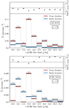 |
Fig. 10. Same as Fig. 7, but for z > 3. |
| In the text | |
|
Fig. 11. Simulated z > 6 AGN to be detected by SKAO in the three tiers of its continuum 1.4 GHz surveys. Each point is color-coded according to its obscuration level. The top three panels show the distribution of log L1.4 GHz while the bottom panels show the distribution of log Lbol. The number of simulated sources in the Wide survey panels is almost 1/10 of the number of AGN reported in Table 4 (see text for details). |
| In the text | |
Current usage metrics show cumulative count of Article Views (full-text article views including HTML views, PDF and ePub downloads, according to the available data) and Abstracts Views on Vision4Press platform.
Data correspond to usage on the plateform after 2015. The current usage metrics is available 48-96 hours after online publication and is updated daily on week days.
Initial download of the metrics may take a while.