eROSITA Final Equatorial-Depth Survey (eFEDS)

Kohei Ichikawa; Takuji Yamashita; Andrea Merloni; Junyao Li; Teng Liu; Mara Salvato; Masayuki Akiyama; Riccardo Arcodia; Tom Dwelly; Xiaoyang Chen; Masatoshi Imanishi; Kohei Inayoshi; Toshihiro Kawaguchi; Taiki Kawamuro; Mitsuru Kokubo; Yoshiki Matsuoka; Tohru Nagao; Malte Schramm; Hyewon Suh; Masayuki Tanaka; Yoshiki Toba; Yoshihiro Ueda

doi:10.1051/0004-6361/202244271

Home

All issues

Volume 672 (April 2023)

A&A, 672 (2023) A171

Full HTML

Open Access

Issue		A&A Volume 672, April 2023


Article Number		A171
Number of page(s)		20
Section		Extragalactic astronomy
DOI		https://doi.org/10.1051/0004-6361/202244271
Published online		19 April 2023

A&A 672, A171 (2023)

eFEDS X-ray view of WERGS radio galaxies selected by the Subaru/HSC and VLA/FIRST survey

Kohei Ichikawa (市川幸平)¹^,2^,3, Takuji Yamashita⁴, Andrea Merloni¹, Junyao Li⁵, Teng Liu¹, Mara Salvato¹, Masayuki Akiyama³, Riccardo Arcodia¹, Tom Dwelly¹, Xiaoyang Chen⁶, Masatoshi Imanishi⁴, Kohei Inayoshi⁷, Toshihiro Kawaguchi⁸, Taiki Kawamuro⁹^,4, Mitsuru Kokubo¹⁰, Yoshiki Matsuoka¹¹, Tohru Nagao¹¹, Malte Schramm¹², Hyewon Suh¹³, Masayuki Tanaka⁴, Yoshiki Toba¹⁴^,15^,11 and Yoshihiro Ueda¹⁴

¹ Max Planck Institut für Extraterrestrische Physik, Giessenbachstrasse 1, 85748 Garching bei München, Germany
² Frontier Research Institute for Interdisciplinary Sciences, Tohoku University, Sendai 980-8578, Japan
³ Astronomical Institute, Tohoku University, Aramaki, Aoba-ku, Sendai, Miyagi 980-8578, Japan
e-mail: k.ichikawa@astr.tohoku.ac.jp
⁴ National Astronomical Observatory of Japan, Mitaka, Tokyo 181-8588, Japan
⁵ Department of Astronomy, University of Illinois at Urbana-Champaign, Urbana, IL 61801, USA
⁶ ALMA Project, National Astronomical Observatory of Japan, 2-21-1, Osawa, Mitaka, Tokyo 181-8588, Japan
⁷ Kavli Institute for Astronomy and Astrophysics, Peking University, Beijing 100871, PR China
⁸ Department of Economics, Management and Information Science, Onomichi City University, Hisayamada 1600-2, Onomichi, Hiroshima 722-8506, Japan
⁹ Nućleo de Astronomía de la Facultad de Ingeniería, Universidad Diego Portales, Av. Ejéercito Libertador 441, Santiago, Chile
¹⁰ Department of Astrophysical Sciences, Princeton University, 4 Ivy Lane, Princeton, NJ 08544, USA
¹¹ Research Center for Space and Cosmic Evolution, Ehime University, 2-5 Bunkyo-cho, Matsuyama, Ehime 790-8577, Japan
¹² Graduate school of Science and Engineering, Saitama Univ. 255 Shimo-Okubo, Sakura-ku, Saitama City, Saitama 338-8570, Japan
¹³ Gemini Observatory/NSF’s NOIRLab, 670 N. A’ohoku Place, Hilo, HI 96720, USA
¹⁴ Department of Astronomy, Kyoto University, Kitashirakawa-Oiwake-cho, Sakyo-ku, Kyoto 606-8502, Japan
¹⁵ Academia Sinica Institute of Astronomy and Astrophysics, 11F of Astronomy-Mathematics Building, AS/NTU, No. 1, Section 4, Roosevelt Road, Taipei 10617, Taiwan

Received: 15 June 2022
Accepted: 13 February 2023

Abstract

We constructed the eROSITA X-ray catalog of radio galaxies discovered by the WERGS survey, made by cross-matching the wide area Subaru/Hyper Suprime-Cam (HSC) optical survey and VLA/FIRST 1.4 GHz radio survey. We report finding 393 eROSITA detected radio galaxies in the 0.5−2 keV band in the eFEDS field covering 140 deg². Thanks to the wide and medium depth eFEDS X-ray survey down to f_{0.5 − 2 keV} = 6.5 × 10⁻¹⁵ erg s⁻¹ cm⁻², the sample contains the rare and most X-ray luminous radio galaxies above the knee of the X-ray luminosity function, spanning 44 < log(L_{0.5−2 keV}^(abs,corr)/erg s⁻¹) < 46.5 at 1 < z < 4. The sample also contains the sources around and below the knee for the sources 41 < log(L_{0.5−2 keV}^(abs,corr)/erg s⁻¹) < 45 at z < 1. Based on the X-ray properties obtained by the spectral fitting, 37 sources show obscured active galactic nucleus (AGN) signatures with log(N_H/cm⁻²) > 22. These obscured and radio AGN reside in 0.4 < z < 3.2, indicating that they are obscured counterparts of the radio-loud quasar, which were missed in the previous optical quasar surveys. By combining radio and X-ray luminosities, we also investigated the jet production efficiency η_jet = η_radP_jet/L_AGN,bol by utilizing the jet power of P_jet. We find that there are 14 sources with extremely high jet production efficiency at η_jet ≈ 1. This high η_jet value might be a result of the decreased radiation efficiency of η_rad < 0.1, due to the low accretion rate for those sources, and/or of the boosting due to the decline of L_AGN,bol by a factor of 10−100 by keeping P_jet constant in the previous Myr, indicating the experience of the AGN feedback. Finally, inferring the BH masses from the stellar mass, we find that X-ray luminous sources show the excess of the radio emission with respect to the value estimated from the fundamental plane. This radio emission excess cannot be explained by the Doppler boosting alone, and therefore the disk–jet connection of X-ray luminous eFEDS-WERGS is fundamentally different from the conventional fundamental plane which mainly covers the low-accretion regime.

Key words: galaxies: active / X-rays: galaxies / galaxies: jets / accretion, accretion disks / galaxies: nuclei

© The Authors 2023

Open Access article, published by EDP Sciences, under the terms of the Creative Commons Attribution License (https://creativecommons.org/licenses/by/4.0), which permits unrestricted use, distribution, and reproduction in any medium, provided the original work is properly cited.

This article is published in open access under the Subscribe to Open model. Subscribe to A&A to support open access publication.

1. Introduction

Relativistic jets launched by supermassive black holes (SMBHs) are the most energetic particle accelerators in the universe. The galaxies hosting such radio jets are called radio galaxies¹ or radio active galactic nuclei (AGN). Roughly 10% of the accreting SMBHs or AGN in the local universe are known as radio galaxies (Kellermann et al. 1989; Ivezić et al. 2002; Sikora et al. 2007; Ho 2008); the jets are thought to disturb the surrounding gas, and thus affect the host galaxy evolution by injecting energy and momentum, which results in suppression of star formation (e.g., Fabian 2012).

Local radio galaxies at z < 0.5 have been studied over the last 20 yr as a showcase in the act of “AGN feedback” (Sadler et al. 2002; Best et al. 2005; Mauch & Sadler 2007; Best & Heckman 2012). Thanks to the combination of multiwavelength data including optical, infrared (IR), and X-ray bands, the obtained ubiquitous features are that these radio galaxies are massive galaxies with M_⋆ > 10¹¹ M_⊙ and they show very low star formation rates with the presence of dispersing interstellar medium (Morganti et al. 2005; Holt et al. 2008; Nesvadba et al. 2017) and/or X-ray cavities (e.g., Rafferty et al. 2006; McNamara & Nulsen 2007; Blandford et al. 2019). They are also associated with a low accretion rate onto the SMBHs (i.e., Eddington ratio of λ_Edd < 10⁻²), suggesting that the energy release is dominated by the kinetic power by jets, not by the radiation from AGN accretion disks (e.g., Best & Heckman 2012).

On the other hand, high-z radio galaxies show a different picture. Using over 10³ radio AGN selected from the Very Large Array (VLA)-COSMOS 3 GHz large project (Smolčić et al. 2017a,b), Delvecchio et al. (2018) demonstrated that SMBH accretion in radio AGN are most radiatively efficient (λ_Edd > 10⁻²) at z > 1, and that they reside in star-forming galaxies, which indicates the presence of plentiful cold gas in the host galaxies. They might be tracing a rapidly growing phase of the SMBHs before the AGN feedback, shedding light on understanding the BH growth. This picture of radio AGN is completely different from that seen in the local universe in the same radio luminosity range (e.g., Hickox et al. 2009). Even so, the survey volume of VLA-COSMOS surveys is small with the survey area of 2 deg² so they may be missing a rare but radio-bright population in the redshift range of z > 1. On the other hand, wide area radio surveys such as VLA/FIRST, even though its sensitivity is shallow (> 1 mJy), still miss most of the optical counterparts in the wide-area surveys. Roughly 70% of those radio emitters are optically unknown in the SDSS survey footprint (Ivezić et al. 2002; Helfand et al. 2015), mainly due to the shallow optical depth of the SDSS survey down to only i_AB = 22 mag. Although the combined efforts are conducted in the previous radio surveys, their studies also indicate that wide and deep counterpart searches of these radio emitters is still an unexplored frontier of such “known unknown” sources.

The recent Subaru/Hyper Suprime-Cam (HSC; Miyazaki et al. 2018) strategic survey program (hereafter HSC-SSP) opens the wide-field optical photometric view with unprecedented depth down to i_AB ∼ 26 for a wide area (∼1100 deg² as of January 2022). We conducted a search for optically faint radio galaxies (RGs) using the Subaru HSC survey catalog (Aihara et al. 2018a) and the VLA/FIRST 1.4 GHz radio catalog, and we found a large number (> 3 × 10³ sources) of RGs at z ∼ 0 − 6 (Yamashita et al. 2018, 2020; Uchiyama et al. 2022a,b). The project is called Wide and deep Exploration of Radio Galaxies with Subaru/HSC (WERGS; Yamashita et al. 2018). They also demonstrated that over 60% of VLA/FIRST radio populations now have reliable optical counterparts thanks to deep HSC/optical imaging². Toba et al. (2019) compiled multiwavelength data covering the optical and IR of the WERGS sample. By utilizing the multiwavelength data, Ichikawa et al. (2021) showed that some WERGS radio galaxies with high radio loudness would harbor a unique type of AGN. These WERGS sources are prominent candidates of very rapidly growing black holes reaching Eddington-limited accretion, and such an accretion phase might accompany the powerful jet activity (e.g., Tchekhovskoy et al. 2011).

X-ray observations provide another important view of these radio galaxies. The X-ray emission is thought to arise from a hot electron corona above the accretion disk (Haardt & Maraschi 1991) and is predominantly produced by the inverse Compton scattering of photons from the accretion disk, that is, a tracer of the AGN accretion disk luminosity. This argument is largely true also for most of the radio galaxies, except blazars that produce a strong contribution of jets in the X-ray band (e.g., Inoue & Totani 2009; Ghisellini et al. 2017). Previous X-ray surveys, primarily with Chandra and XMM-Newton, have made remarkable progress in the study of accretion onto SMBHs across the cosmic epoch in the universe (Merloni et al. 2014; Ueda et al. 2014; Brandt & Alexander 2015; Buchner et al. 2015). However, the X-ray properties of radio galaxies across the universe are still poorly known, especially in the high-z universe at z > 1, for a combination of the two reasons. The first is that the number density of radio galaxies is one order of magnitude smaller than radio-quiet AGN (e.g., Ivezić et al. 2002), so they are very rare, and therefore X-ray surveys with large fields of view (FoVs) are needed to uncover this population. The second reason is the lack of such X-ray survey achieving both wide-area (> 100 deg²) and medium deep X-ray sensitivity (f_0.5-2 keV < 10⁻¹⁴ erg s⁻¹ cm⁻²; see, e.g., Merloni et al. 2012). Therefore, most of the WERGS sample solely relied on the shallow WISE mid-IR bands for the estimation of the radiation power from the AGN (Toba et al. 2019; Ichikawa et al. 2021).

The extended ROentgen Survey with an Imaging Telescope Array (eROSITA; Predehl et al. 2021) on board the Spektrum-Roentgen-Gamma mission (SRG; Sunyaev et al. 2021) provides an unprecedented very wide FoV of X-ray imaging and spectroscopy thanks to its large collecting area and high grasp (collecting area × FoV). The eROSITA surveys the sky (the eROSITA All-Sky Survey: eRASS; Predehl et al. 2021) in the two energy bands, the soft (0.2−2.3 keV) and hard (2.3−8 keV) bands. In the soft X-ray band the eROSITA survey will be about 25 times more sensitive than the ROSAT all-sky survey (Truemper 1993), while in the hard band it will provide the first ever true imaging all-sky survey at those energies.

To demonstrate the ground-breaking survey capabilities of eROSITA and to maximize the science exploitation of the uninterrupted eRASS program, the eROSITA team observed the contiguous 140 deg² field called eROSITA Final Equatorial-Depth Survey (eFEDS; Brunner et al. 2022) during the SRG and performance verification phase, between 2019 November 3 and 7, reaching a flux limit of f_0.5-2 keV = 6.5 × 10⁻¹⁵ erg s⁻¹ cm⁻², which is 50% deeper than the final integration of the planned four-year program (eRASS8) in the ecliptic equatorial region (f_0.5-2 keV = 1.1 × 10⁻¹⁴ erg s⁻¹ cm⁻²Predehl et al. 2021); therefore, eFEDS is considered to be a representation of the final eROSITA all-sky survey. In addition, the 0.5−2 keV flux limit of eFEDS is significantly deeper than the expected limit estimated from the WISE W3 (12 μm) band flux density limit, where f_ν, lim = 1 mJy corresponds to f_{0.5 − 2 keV} = 8.3 × 10⁻¹⁴ erg s⁻¹ cm⁻², by assuming the local X-ray–mid-infrared (MIR) luminosity correlation of AGN (Gandhi et al. 2009; Asmus et al. 2015; Ichikawa et al. 2012, 2017, 2019a) and by assuming the X-ray photon index of Γ = 1.8 (e.g., Ricci et al. 2017). Another advantage of the eFEDS field is its location of GAMA09 field, where multiwavelength surveys are already conducted, including the DESI Legacy Survey (Dey et al. 2019) and the Subaru/HSC SSP optical survey (Aihara et al. 2018a).

In this study we explore the AGN and host galaxy properties of the eROSITA-detected X-ray bright radio galaxies in the eFEDS field, selected by the combination of the eROSITA/eFEDS, Subaru/HSC optical, and VLA/FIRST radio surveys. The joint effort between the eROSITA and Subaru/HSC teams enabled us to explore the HSC five-band optical imaging and photometries for most of the eFEDS field. Throughout this paper we use the AB magnitude system in the optical bands, and we adopt the same cosmological parameters as Yamashita et al. (2018): H₀ = 70 km s⁻¹ Mpc⁻¹, Ω_M = 0.27, and Ω_Λ = 0.73. This paper is part of the eFEDS paper series, and it is also labeled as the eighth paper in the WERGS paper series.

2. Sample selection and properties

We here describe the eFEDS detected radio galaxy catalog (eFEDS-WERGS) based on the cross-matching between the VLA/FIRST radio surveys and the optical counterparts of the eFEDS X-ray sources. The HSC-SSP currently covers > 10³ deg² region including most of the eFEDS area. We refer to Yamashita et al. (2018) for the original S16A-WERGS catalog and Toba et al. (2019) and Ichikawa et al. (2021) for the IR catalog of the WERGS sample.

2.1. VLA/FIRST

The VLA/FIRST survey contains radio continuum imaging data at 1.4 GHz with a spatial resolution of 5.4 arcsec (or ≲40 kpc at z ∼ 1 − 4; Becker et al. 1995; White et al. 1997), which completely covers the footprint of the HSC-SSP Wide-layer (see below). Following the same method with Yamashita et al. (2018), who utilized the final release catalog of FIRST (Helfand et al. 2015) with the flux limit of > 1 mJy, we extracted 12 375 FIRST sources in the eFEDS footprint.

2.2. eFEDS

2.2.1. eFEDS X-ray and optical counterpart catalog

The eROSITA team compiled the eFEDS X-ray source catalog (Brunner et al. 2022), which contains the 27 910 X-ray point sources with a detection likelihood at 0.2−2.3 keV of DET_LIKE > 6, which corresponds to the significant detection with limiting flux of f_0.5-2 keV = 6.5 × 10⁻¹⁵ erg s⁻¹ cm⁻². Of these sources, 27 369 X-ray point sources show no extended signature with EXT_LIKE = 0. This catalog gives a secured signal-to-noise ratio as the detection, and the estimated spurious detection rate is around 3%.

The counterparts are presented in Salvato et al. (2022) and they were identified using the DESI Legacy Survey Data Release 8 (LS8; Dey et al. 2019), which covers the northern hemisphere and the whole eFEDS field in three optical bands (g, r, and z) using telescopes at the Kitt Peak National Observatory and the Cerro Tololo Inter-American Observatory. The main reason for using LS8 in Salvato et al. (2022) is that LS8 covers the field homogeneously and has sufficient depth, based on the expected optical properties of the X-ray population.

Two independent methods were used and compared for the counterpart identifications: NWAY (Salvato et al. 2018) and ASTROMATCH (Ruiz et al. 2018). Both methods make use of a large training sample of X-ray sources with secure counterparts to determine different complex priors. Both methods provide high completeness and purity, but NWAY provides a larger fraction of correct counterparts and a smaller fraction of sources for which the identification of the counterparts is not unique (see Salvato et al. 2018, for details). The identification of the counterparts was finalized by comparing the solutions provided by the two methods, especially based on the respective probability values of the right counterparts. Then, a flag was assigned to each source with the ranking of reliability (see Salvato et al. 2022, for more details). In this study we use only the sources that have reliable optical counterparts with CTP_quality ≧ 2, where both NWAY and ASTROMATCH methods give the same counterparts, and securely extra-galactic sources with CTP_CLASS ≧ 2 (see Salvato et al. 2022). This reduces the sample size to 21 952.

In the catalog Salvato et al. (2022) also compiles the high spatial resolution Subaru/HSC photometries obtained by the Subaru/HSC SSP survey. The Subaru/HSC-SSP is an ongoing wide and deep imaging survey covering five broadband filters (g-, r-, i-, z-, and y-band; Aihara et al. 2018a; Bosch et al. 2018; Furusawa et al. 2018; Kawanomoto et al. 2018; Komiyama et al. 2018; Huang et al. 2018), consisting of three layers (Wide, Deep, and UltraDeep). Salvato et al. (2022) utilized the Wide-layer S19A data release, which covers almost the entire eFEDS footprint. The forced photometry of 5σ limiting magnitude reaches 26.8, 26.4, 26.4, 25.5, and 24.7 for the g, r, i, z, and y-band, respectively (Aihara et al. 2018b). The average seeing in the i-band is 0.6 arcsec, and the astrometric root mean square uncertainty is about 40 mas. After removing spurious sources flagged by the pipeline, Salvato et al. (2022) cross-matched the HSC sources with a search radius of 1 arcsec (for more details on the HSC photometric catalog in the eFEDS field, see also Salvato et al. 2022; Toba et al. 2022).

Salvato et al. (2022) also gathered the optical spectroscopic data for obtaining the spec-z. The eFEDS field was previously observed by several spectroscopic surveys, mostly by SDSS I−IV (Ahumada et al. 2020), GAMA (DR3; Baldry et al. 2018), WiggleZ (final data release; Drinkwater et al. 2018), 2SLAQ (Croom et al. 2009), 6dFGS (final data release; Jones et al. 2009), LAMOST (DR5; Luo et al. 2015), and Gaia RVS (DR2; Gaia Collaboration 2018). Most of the existing spectra are of high enough quality for the spec-z measurements and source classification to separate the stars, quasars, and/or galaxies. The sources with good-quality spec-z are classified as CTP_REDSHIFT_GRADE = 5 in the optical counterpart catalog (for more details, see Salvato et al. 2022).

The catalog also contains photo-z information. The computation of the photo-z follows that of Salvato et al. (2009, 2011) using the LePhare code (Arnouts et al. 1999; Ilbert et al. 2006), with the aid of the multiwavelength photometries covering from optical to IR, and fed by the comparison of the independent photometric redshift method DNNz (Nishizawa et al. 2020) for the photometric redshift grade evaluation. We utilized the redshift quality of CTP_REDSHIFT_GRADE ≧ 3, whose sources have consistent photo-z values between the LePhare and DNNz codes or have high photo-z reliability. This reduces the total number of the sample to 20 850. Out of the sample, 5284 sources have spec-z and the remaining 15 566 sources have photo-z (see Salvato et al. 2022 for more details).

2.2.2. eFEDS X-ray spectral fitting catalog

After the identification of the optical counterpart and the obtained redshift information, eROSITA team further analyzed their X-ray spectra properties. Liu et al. (2022) compiled the X-ray fitting catalog for 21 952 sources with reliable counterparts and with good signal-to-noise ratios, and then performed the simple spectral X-ray fitting with XSPEC terminology of TBabs*zTBabs*powerlaw (Liu et al. 2022), where the power-law (powerlaw) index (Γ) is set as free with the prior distribution centered at Γ = 2.0 with σ = 0.5, and log-uniform prior for the column density N_H (zTBabs) with 4 × 10¹⁹ < N_H/cm⁻² < 4 × 10²⁴. The galactic absorption (TBabs) is also applied using the total N_H, Gal measured by the neutral HI observations through the H4PI Collaboration (HI4PI Collaboration 2016) in the direction of the eFEDS field. Utilizing the obtained redshift information by Salvato et al. (2022), Liu et al. (2022) derived key AGN properties, including the absorption corrected rest-frame 0.5−2.0 keV ( $L_{0.5 - 2 keV}^{(abs, corr)}$ ${L_{0.5{-}2\,{\rm keV}}^{\rm (abs,corr)}}$ ) and the 2−10 keV X-ray luminosities ( $L_{2 - 10 keV}^{(abs, corr)}$ ${L_{2{-}10\,{\rm keV}}^{\rm (abs,corr)}}$ ), the column density (N_H), and X-ray spectral index (Γ). In this study we limit the sample only to reliable spec-z and photo-z measurements (as discussed in Sect. 2.2.1) and reliable spectral fitting with N_H measurements of NHclass ≧ 2. This reduces the sample to 17 603 sources. This is the “parent eFEDS catalog” used for the cross-matching in Sect. 2.3.

2.3. Cross-matching with parent eFEDS catalog

The parent eFEDS catalog already contains both LS8 and HSC optical counterpart information; therefore, we apply a simpler cross-matching between the FIRST radio sources and the eFEDS optical counterpart, instead of the cross-matching between the WERGS catalog in the eFEDS footprint and eFEDS optical counterparts. Although the original WERGS catalog should follow the latter approach, this method misses optically bright sources i_AB < 18 where Subaru/HSC optical bands show a saturation (Tanaka et al. 2018; Yamashita et al. 2018). On the other hand, the former approach has a great advantage without losing the optically bright sources since LS8 could cover reliable photometries instead.

We cross-matched the FIRST radio sample with the parent eFEDS catalog with the nearest matching within the 1 arcsec cross-matching radius. We used the VLA/FIRST coordinates (RA and Dec) and optical LS8 best counterpart coordinates (BEST_LS8_RA and BEST_LS8_Dec) for the parent eFEDS catalog. After the cross-matching, 558 sources were left. We confirm that the probability of incorrect identification with unassociated FIRST sources is negligible based on the current nearest cross-matching. The estimated number of false identifications in the sample is 0.37³ within the radius of the 1 arcsec for the searched ∼10⁴ FIRST sources in the eFEDS footprint.

We then applied additional cuts to this sample. We first applied removing possible side-lobe artifacts by utilizing SIDEPROB < 0.05 (Helfand et al. 2015). This reduces the sample size to 504. We then set the radio-loudness cut since our target is radio galaxies whose radio emission should originate from AGN–jet activity, not from the star formation in the host galaxies. Radio loudness is a useful tool to distinguish between radio-quiet and radio-loud AGN, and the observed radio loudness ℛ_obs is defined as log ℛ_obs = log(F_int/F_i-band), where F_int is the total integrated flux density in the FIRST band and F_i-band is the cmodel flux density in the Subaru/HSC band. In this study we set ℛ_obs > 10 (Ivezić et al. 2002; Kellermann et al. 1989). This cut further reduces the sample to 429. We note that the radio-loudness cut does not fully exclude the radio-quiet AGN population (e.g., Sikora et al. 2007; Ho 2008; Chiaberge & Marconi 2011), whose radio loudness sometimes reach ℛ_obs ≃ 100. Thus, our sample possibly contains the radio-quiet AGN population, especially at the low radio luminosity end. On the other hand, as shown in Sect. 3.1.2, our selection cut provides that all of our sources have L_1.4 GHz > 10²³ W Hz⁻¹, whose radio emission is difficult for the host galaxy star formation alone to reach (e.g., Kimball et al. 2011; Padovani 2016; Tadhunter 2016).

Next, we limit our sample to compact sources in the radio band. This is important in order to reduce false optical identification by mismatching the optical sources with the locations of spatially extended radio-lobe emission. We follow the same method as the previous WERGS series (Yamashita et al. 2018; Ichikawa et al. 2021) using the ratio of the total integrated radio flux density to the peak radio flux density f_int/f_peak. They treated the source as compact if the ratio fulfills either of the two following equations,

$\begin{matrix} f_{int} / f_{peak} < 1 + 6.5 \times {(f_{peak} / rms)}^{- 1}, \end{matrix}$ $\begin{aligned}&f_{\rm int}/f_{\rm peak} < 1 + 6.5 \times (f_{\rm peak}/\mathrm{rms})^{-1},\end{aligned}$ (1)

$\begin{matrix} log (f_{int} / f_{peak}) < 0.1, \end{matrix}$ $\begin{aligned}&\log (f_{\rm int}/f_{\rm peak}) < 0.1, \end{aligned}$ (2)

where f_peak/rms is the S/N and rms is the local rms noise in the FIRST catalog; these two equations are from the study by Schinnerer et al. (2007; see also the original criterion in Ivezić et al. 2002). This reduces the final sample to 393 sources. The sources are shown as blue-filled circles in the ℛ_obs − i_AB plane in Fig. 1.

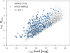Fig. 1.

Logarithmic value of radio loudness (log ℛ_obs = log(F_int/F_i-band)) vs. the observed i_AB band magnitude of our sample (see Sect. 2.3 for the definition). The original WERGS sample (3579 sources) from Yamashita et al. (2018) are shown as gray circles. The finally selected 393 eFEDS-WERGS sources are shown as blue circles. The eFEDS-WERGS sources with spec-z are highlighted with gray open squares. The statistical errors of both values are vanishingly small, and are therefore not shown.

We also investigated how much our radio compact source selection would affect the radio luminosity bias in the sample. In general, the selection of the smaller radio sizes tends to be radio fainter (and therefore could potentially be younger than other radio AGN) as reported in the FR0 sources (e.g., Baldi et al. 2015, 2018) and some radio compact sources in the local universe (e.g., Capetti et al. 2017; Jimenez-Gallardo et al. 2019). In our case the sample shows that the mean radio luminosities are almost comparable between the two subsamples of extended and compact, with ⟨log(L_1.4 GHz/W Hz⁻¹)⟩ = 25.6 ± 1.0 for the extended and ⟨log(L_1.4 GHz/W Hz⁻¹)⟩ = 25.5 ± 1.1 for the compact sources. Therefore, we conclude that our sample selection limited to the radio compact sources generally does not affect the main results hereafter.

2.4. Additional analysis and physical quantities

2.4.1. Luminosities

While the X-ray luminosities are already calculated for all sources in this study (Liu et al. 2022), we summarize here how other luminosities are calculated for other energy bands. The 1.4 GHz radio luminosities (L_1.4 GHz) are calculated by following the same method used in the WERGS catalog (Yamashita et al. 2018; Ichikawa et al. 2021), in which the integrated flux density (f_int) in the VLA/FIRST catalog (Helfand et al. 2015) is used, and k-correction is applied by assuming the power-law radio spectrum with f_ν ∝ ν^α, and α = −0.7 is used for this study (e.g., Condon 1992). The uncertainty of the radio luminosities mainly originates from the assumed α, which actually varies source by source. Although there are very steep spectral sources with α < −1.0 (Komissarov & Gubanov 1994) and flat spectral or very young AGN sources show α > −0.5 (Blundell et al. 1999), most of the radio galaxies are within the range of −1 < α < −0.5 (de Gasperin et al. 2018; Toba et al. 2019). This uncertainty of α produces maximum uncertainty of 0.2 dex in the luminosity, and thus we add the conservative (i.e., overestimated) uncertainty of 0.2 dex to the obtained 1.4 GHz luminosities.

The IR luminosities are also calculated by using the obtained IR fluxes from the WISE all-sky survey (Wright et al. 2010). The eFEDS optical counterpart catalog already compiles the “unWISE” flux with a unit of nanomaggie (Schlafly et al. 2019). We adopted the quality flag of FRAC_FLUX < 0.5, which is the same as in Toba et al. (2022), to avoid the sources with a severe flux contribution from their neighborhoods, which reduces the total available sample from 393 to 323, 345, 198, and 46 source at W1 (3.4 μm), W2 (4.6 μm), W3 (12 μm), and W4 (22 μm) band, respectively. The obtained flux is first converted into the flux density at each band, and then the k-correction is applied to shift to the rest-frame flux densities by assuming a typical AGN IR SED template obtained by Mullaney et al. (2011). The rest-frame band luminosities (L_3.4 μm, L_4.6 μm, L_12 μm, L_22 μm) in the unit of erg s⁻¹ are calculated based on these rest-frame flux densities. The 6 μm IR luminosity is also calculated by assuming the SED of Mullaney et al. (2011), with the conversion factor of L_6 μm = L_12 μm/1.74. Considering the measurement error of WISE band is always vanishingly small, with ΔW? < 0.01 mag (? = 1, 2, 3, 4) for most of the sources, the scatter of the obtained IR luminosities are dominated from the uncertainty of the k-correction based on the assumed AGN SED, which is around 0.2−0.3 dex (Mullaney et al. 2011). Therefore, we add 0.3 dex undertainties to all the IR luminosity errors.

The bolometric AGN luminosities (L_AGN,bol) are estimated from $L_{2 - 10 keV}^{(abs, corr)}$ ${L_{2{-}10\,{\rm keV}}^{\rm (abs,corr)}}$ in Liu et al. (2022) by using the luminosity dependent bolometric correction of Marconi et al. (2004). For the sources with low S/N, $L_{2 - 10 keV}^{(abs, corr)}$ ${L_{2{-}10\,{\rm keV}}^{\rm (abs,corr)}}$ are extrapolated from $L_{0.5 - 2 keV}^{(abs, corr)}$ ${L_{0.5{-}2\,{\rm keV}}^{\rm (abs,corr)}}$ on the fixed power law, and therefore the constant conversion factor of $L_{2 - 10 keV}^{(abs, corr)} / L_{0.5 - 2 keV}^{(abs, corr)} = 1.16$ ${L_{2{-}10\,{\rm keV}}^{\rm (abs,corr)}}/{L_{0.5{-}2\,{\rm keV}}^{\rm (abs,corr)}}=1.16$ (see details in Liu et al. 2022). We also confirmed that the bolometric luminosities are almost same within the scatter of σ = 0.5 dex, even if L_12 μm is utilized by assuming the conversion of L_AGN,bol ≃ 2 L_AGN, IR (Delvecchio et al. 2014; Inayoshi et al. 2018) and L_AGN, IR/L_12 μm = 2.33 (Mullaney et al. 2011).

2.4.2. Two-dimensional image decomposition

To obtain the host galaxy properties, such as the stellar-mass and radial profile, we performed the 2D image decomposition utilizing the high spatial resolution HSC optical images of the final sample. We followed the same method as Li et al. (2021, 2023), who recently conducted the HSC image decomposition of the SDSS quasars at z < 0.8 based on the image modeling tool originally optimized for the lensing detection (Birrer et al. 2015; Birrer & Amara 2018). We briefly summarize the analysis here. We first chose the HSC i-band among the five HSC optical bands as a fiducial frame for the image decomposition. We then performed the 2D brightness-profile fitting using one point spread function (representing the point source) and one single elliptical Sersic model (representing the host galaxy), and determined the galactic structural properties including the Sersic index (n) and the half-light radius (R_e). The final best-fit model image is measured by using the χ² minimization with the particle-swarm optimization algorithm.

We also obtained the host properties by utilizing the decomposed host galaxy emission at grizy bands. We used the SED fitting code CIGALE (Boquien et al. 2019) to derive stellar mass M_⋆ and rest-frame colors of the AGN host galaxies. We applied the model SEDs with a delayed star formation history, the stellar-sysnthesis model of Bruzual & Charlot (2003), a Chabrier (2003) initial mass function, and a Calzetti et al. (2000) attenuation law.

One limitation of image decomposition with the combination of the HSC image is that its application returns the reasonable fitting only up to z < 1, beyond which the morphology information is hard to obtain because the surface brightness dimming produces lower values of the host-to-total flux ratios that make the host galaxy challenging to detect even for the deep HSC data (Ishino et al. 2020; Li et al. 2021). We follow the same method as Li et al. (2021), using these morphological parameters for objects at z < 1.0 with reduced χ² < 5 to ensure reliable host properties. This leaves 139 sources.

In summary, our sample contains 393 sources spanning a redshift range up to 0 < z < 6; 391 out of them are at z < 4. The sample consists of the reliable redshift information: 180 spec-z confirmed sources and 213 reliable photo-z estimations. The total sample (393 sources) covers X-ray and radio luminosities as well as the column density N_H measurements, supplemented by the IR luminosities obtained by WISE (198 sources at W3). Especially at low-z sources at z < 1, 139 sources in the sample have host galaxy properties (such as stellar mass) thanks to the image decomposition technique utilizing the high spatial resolution optical images of Subaru/HSC.

3. Results and discussion

3.1. Basic sample properties

3.1.1. ℛ_obs versus i_AB-band magnitude

Figure 1 shows the distribution of ℛ_obs as a function of the observed i_AB magnitude. The gray point shows the WERGS sample (e.g., Yamashita et al. 2018), spanning down to i_AB ∼ 26, but has a saturation limit at i_AB ∼ 18, as discussed in Sect. 2.3. The eFEDS detected WERGS sources are mainly clustered at 16 < i_AB < 22 (337 out of 393 sources) with a median of ⟨i_AB⟩ = 20.1 ± 1.5, and with a small fraction of sources down to 22 < i_AB < 24.6 (56 sources). The sources enclosed by the open square are spec-z sources; over half of the sources have spec-z information down to i_AB ∼ 21 (completeness of 61%), thanks to the power of SDSS IV spectroscopic follow up (Merloni et al., in prep.).

3.1.2. L − z plane

Figure 2 shows 1.4 GHz, absorption corrected 0.5−2 keV, and 12 μm luminosities of our sample as a function of redshift at 0 < z < 4⁴. The top panel of Fig. 2 shows how uniquely eFEDS-WERGS covers the plane of L_1.4 GHz − z. Our eFEDS-WERGS sample covers relatively high radio luminosities with a median of ⟨log(L_1.4 GHz/W Hz⁻¹)⟩ = 25.5, which is roughly two orders of magnitude brighter than the overall VLA-COSMOS sources with significant X-ray detections (VLA-COSMOS-X, ⟨log(L_1.4 GHz/W Hz⁻¹)⟩ = 23.6; Smolčić et al. 2017a,b) across the redshift range of 0 < z < 4, indicating that most of our sample is composed of rare and radio-powerful AGN, thanks to the wide area coverage of eFEDS-WERGS sample with > 100 deg².

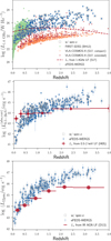Fig. 2.

Luminosities of eFEDS-WERGS sample as a function of redshift. The points are the same as in Fig. 1. Top: rest-frame radio luminosity log L_1.4 GHz (W Hz⁻¹) as a function of redshift, where L_1.4 GHz is obtained from VLA/FIRST (Helfand et al. 2015), and the k-correction was made by Yamashita et al. (2018) based on redshift. The green stars and orange circle and red star points are data obtained from the FIRST-SDSS (Best & Heckman 2012) and VLA-COSMOS catalog, respectively. Middle: 0.5−2 keV AGN luminosity ( $L_{0.5 - 2 keV}^{(abs, corr)}$ ${L_{0.5{-}2\,{\rm keV}}^{\rm (abs,corr)}}$ ) as a function of redshift. The red-filled circle with error bar represents the break luminosity at 0.5−2 keV obtained from Hasinger et al. (2005). Bottom: 12 μm luminosity L_12 μm (erg s⁻¹) as a function of redshift. The k-correction is made by assuming the AGN SED of Mullaney et al. (2011). The red filled circle with error bar represents the break luminosity estimated from the IR AGN studies (Delvecchio et al. 2014).

We also investigate the impact of the radio observation baseline differences on the luminosity discrepancy between our eFEDS-WERGS sample and the VLA-COSMOS-X. While the VLA-FIRST (and therefore the eFEDS-WERGS) sources are based on observations from the VLA in its B-configuration, the VLA-COSMOS(-X) sample is constructed from VLA observations in the longer A configurations and supplementary observations in the shorter C configurations. As demonstrated by Smolčić et al. (2017a), the VLA-COSMOS(-X) sources are classified as radio-extended or compact based on the flux ratio of total to peak radio flux, and its total flux is complimented by their C-configuration observations. The top panel of Fig. 2 shows that although the radio-extended or VLA-COSMOS-X sources (red stars) have higher radio luminosities of ⟨log(L_1.4 GHz/W Hz⁻¹)⟩ = 23.9 compared to the radio-compact VLA-COSMOS sources (orange stars) with ⟨log(L_1.4 GHz/W Hz⁻¹)⟩ = 23.5. However, this difference does not fill in the gap in radio luminosity between the eFEDS-WERGS and VLA-COSMOS-X.

Figure 2 (top panel) also shows the comparison from the sample by the FIRST-SDSS survey (Best & Heckman 2012). Our sample covers high-z sources (⟨z⟩ = 1.1 for eFEDS-WERGS, and ⟨z⟩ = 0.2 for the FIRST-SDSS sources) thanks to the deeper X-ray follow-ups and the SDSS IV spectroscopic survey, and thanks to the power of deep photometries of Subaru/HSC. The red dashed line represents the 1.4 GHz break luminosity of lower-power radio AGN, which is obtained from the 1.4 GHz luminosity function studies by Smolčić et al. (2017a). More than half of the sources are located above the line of the break luminosity at z > 1.0, and almost all of them are located at z > 1.5. This indicates that eFEDS-WERGS are relatively rare, and therefore radio luminous AGN. Their luminosity range is similar to the high radio luminosity AGN populations such as FR I (10²⁵ < L_1.4 GHz/W Hz⁻¹ < 3 × 10²⁶) and FR II (mainly with L_1.4 GHz > 3 × 10²⁶ W Hz⁻¹; Dunlop & Peacock 1990; Willott et al. 2001).

The middle panel of Fig. 2 shows the absorption corrected 0.5−2 keV X-ray luminosity ( $L_{0.5 - 2 keV}^{(abs, corr)}$ ${L_{0.5{-}2\,{\rm keV}}^{\rm (abs,corr)}}$ ) as a function of z. The red filled circle represents the break 0.5−2 keV AGN luminosity (L_{⋆, 0.5 − 2 keV}) at each redshift obtained from Hasinger et al. (2005). This clearly shows that our sample covers the relatively rare and luminous end of the X-ray AGN at z > 1 and covers the sources around the shoulder at 0.2 < z < 1, thanks to the wide coverage of eFEDS field. We discuss the possible jet contamination in the X-ray band in Sect. 3.3.

One notable trend in the middle panel of Fig. 2 is that eFEDS-WERGS catalog contains the most X-ray luminous radio AGN exceeding $L_{0.5 - 2 keV}^{(abs, corr)} > 10^{45.5}$ ${L_{0.5{-}2\,{\rm keV}}^{\rm (abs,corr)}} > 10^{45.5}$ erg s⁻¹. Even limiting the sample with the spec-z sources, there are seven sources above $L_{0.5 - 2 keV}^{(abs, corr)} > 10^{45.5}$ ${L_{0.5{-}2\,{\rm keV}}^{\rm (abs,corr)}} > 10^{45.5}$ erg s⁻¹, two of which are above $L_{0.5 - 2 keV}^{(abs, corr)} > 10^{46}$ ${L_{0.5{-}2\,{\rm keV}}^{\rm (abs,corr)}} > 10^{46}$ erg s⁻¹, whose expected bolometric luminosity reaches L_AGN,bol ≃ 10⁴⁸ erg s⁻¹, which is equivalent to the Eddington limit luminosity of maximum mass SMBHs with M_BH = 10¹⁰ M_⊙ (e.g., Kormendy & Ho 2013). This suggests that they are a promising candidate population for the super-Eddington phase, and the association of strong 1.4 GHz emission indicates that the super-Eddington phase is somehow linked to the jet emission. Although we cannot discard the possibility that they are also blazars, and therefore both radio and X-ray emission is boosted by jet, these sources are not listed in the eFEDS-blazar catalog (Collmer et al., in prep.) based on the cross-matching to the optical counterparts of previously known blazar catalogs such as BZCAT (Massaro et al. 2015) and gamma-ray detected blazars. In addition, the archival SDSS spectra show that at least three sources show quasar-like spectra, showing a broad Lyα and CIV emission with a blue continuum, suggesting that the accretion disk emission is dominated at least in the optical band.

The bottom panel of Fig. 2 shows the rest-frame 12 μm luminosity as a function of z, which is considered to be mainly dominated by AGN dust emission (e.g., Gandhi et al. 2009; Asmus et al. 2015; Ichikawa et al. 2017). The red-filled circles represent the break 12 μm AGN luminosity (L_{⋆, 12 μm}) at each redshift obtained from Delvecchio et al. (2014), who compiled the break AGN bolometric luminosities from the IR SED fitting, with the combination of the bolometric correction of L_AGN, bol/L_AGN, TIR ≃ 3 (Delvecchio et al. 2014) and the 12 μm to total IR AGN conversion factor of L_⋆(TIR)/L_⋆(12 μm) = 2.3 (Mullaney et al. 2011; Ichikawa et al. 2019a). Again, our sample is located above the break luminosity of IR AGN luminosity function (Delvecchio et al. 2014), indicating that our eFEDS-WERGS sample covers the relatively rare and luminous end of AGN population at z > 0.5, and the sample is located around the break luminosity at z < 0.5. This illustrates a slight difference in the location of AGN luminosities between the X-ray and MIR bands at z < 1, where most of the 12 μm sources are located on or above the shoulder at 0.5 < z < 1. This seemingly discrepant location might be a result of the contamination from the host galaxies into the 12 μm band, which is sometimes significant, especially at the lower luminosity end at L_12 μm < 10⁴⁴ erg s⁻¹ (Ramos Almeida et al. 2009; Alonso-Herrero et al. 2011; Ichikawa et al. 2015). We discuss this point in Sect. 3.3.

To summarize, Fig. 2 illustrates two important properties. One is that the eFEDS-WERGS sample at z < 1 covers the sources around the break luminosity of each luminosity function in each wavelength band. The second is that the sample at 1 < z < 4 covers the sources above the break luminosities, indicating that they are rare and luminous AGN populations in radio, X-ray, and IR bands at each redshift range in 1 < z < 4.

3.2. Obscuration properties

The X-ray spectral analysis provides N_H, which is an indicator of obscuring gas properties around AGN. eROSITA already discovered statistically large number of obscured (N_H > 10²² cm⁻²) AGN at z > 0.5 in the eFEDS field (Brusa et al. 2022; Toba et al. 2022). As already discussed in Liu et al. (2022), we note that the uncertainty of N_H is not small, reaching Δ log(N_H/cm⁻²) = 0.67 for the sample (see top right panel of Fig. 3). In this study, we use the best-fit N_H as a face value, but we note that the large uncertainty always harbors the possibility that unobscured AGN might be obscured ones, and vice versa if the source is around log(N_H/cm⁻²) ∼ 22.

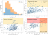Fig. 3.

Obscuration properties of the eFEDS-WERGS sample. Top left: histogram of log(N_H/cm⁻²). The sources are divided into two subgroups with spec-z (cyan) and phot-z (orange). Top right: log N_H as a function of redshift. The gray error bar shows a typical logarithmic error of log N_H. Bottom left: log N_H as a function of 0.5−2 KeV X-ray luminosity ( $L_{0.5 - 2 keV}^{(abs, corr)}$ ${L_{0.5{-}2\,{\rm keV}}^{\rm (abs,corr)}}$ ). The orange shaded area represents the region of obscured AGN with log(N_H/cm⁻²) > 22. The symbols are same as in Fig. 1, and the gray error bar shows a typical logarithmic error of log N_H and log $L_{0.5 - 2 keV}^{(abs, corr)}$ ${L_{0.5{-}2\,{\rm keV}}^{\rm (abs,corr)}}$ . Bottom right: relation between the flux density ratio of 12 μm to optical i_AB band and the log (N_H/cm⁻²). The dashed black line represents the slope of the fitting. The red shaded area represents the region of extremely red quasars which fulfill f_ν(12 μm)/f_ν, i-band > 10^1.84 (Hamann et al. 2017). The orange shaded area represents the obscured AGN region. The other symbols are the same as in Fig. 1.

The top left panel of Fig. 3 shows the histogram of N_H of our sample, divided by the spec-z and photo-z sample; it illustrates that most of the eFEDS-WERGS sources can be classified as unobscured AGN with log(N_H/cm⁻²) < 22, comprising 91% of the sources (356 out of 393 sources). This is a natural outcome considering that eROSITA is more sensitive in the soft 0.5−2 keV band, which is weak against the strong absorption with log(N_H/cm⁻²) > 22 (e.g., Merloni et al. 2012; Ricci et al. 2015; Liu et al. 2022). This means that 91% of our eFEDS-WERGS sources are unobscured radio-loud AGN. Considering that most of them at z > 1 have the luminosity range of $log (L_{0.5 - 2 keV}^{(abs, corr)} / erg s^{- 1}) > 44$ $\log ({L_{0.5{-}2\,{\rm keV}}^{\rm (abs,corr)}}/{\rm erg}\,{\rm s}^{-1})>44$ (93% or 123 out of the 132 unobscured AGN at z > 1), they are likely radio-loud quasars.

While they are rare, 9% of the population (37 out of the 393 sources) shows a strong absorption reaching log(N_H/cm⁻²) > 22.0. The top right panel of Fig. 3 shows that most of those obscured AGN are distributed widely at 0.4 < z < 3.2, which is slightly biased to high-z values. It is a natural outcome since the observed 0.5−2 keV covers a higher energy band that is stronger against the gas absorption at higher redshift. This produces a negative k-correction, and thus the observed energy coverage enables eROSITA to detect relatively obscured AGN.

The bottom left panel of Fig. 3 shows the distribution of N_H as a function of $L_{0.5 - 2 keV}^{(abs, corr)}$ ${L_{0.5{-}2\,{\rm keV}}^{\rm (abs,corr)}}$ . All of the obscured AGN are X-ray luminous, with the median of $〈 log (L_{0.5 - 2 keV}^{(abs, corr)} / erg s^{- 1}) 〉 = 44.6$ $\left\langle \log \left({L_{0.5{-}2\,{\rm keV}}^{\rm (abs,corr)}}/{\rm erg}\,{\rm s}^{-1}\right) \right\rangle = 44.6$ , or ⟨log(L_AGN,bol/erg s⁻¹)⟩ = 46.6, which is a similar luminosity to the optical SDSS quasar (e.g., Shen et al. 2011; Rakshit et al. 2020). This indicates that they are X-ray and radio-luminous obscured AGN. Considering that these sources are located at 0.4 < z < 3.2, they are equivalent to radio SDSS quasars, but with strong absorption, and these populations were widely missed in the previous SDSS optical band studies, showing the power of wide and medium-depth X-ray surveys by eROSITA.

Out of the 37 obscured radio AGN, 15 sources are spec-z confirmed sources, and the SDSS spectra of 9 of these sources are publicly available. Three of the nine sources show clear quasar spectra, and another three sources show a broad emission component either in the Hβ, MgII, or Lyα but with a redder continuum. The remaining three show type 2 AGN-like spectra whose continuum is dominated by the host galaxies. Interestingly, three sources are high-z sources at z > 3. Figure 4 shows both the X-ray (top panel) and optical spectra (bottom panel) of all three spec-z confirmed obscured radio AGN at z > 3 found in this study. Three sources are highly X-ray and radio luminous AGN with $45.0 < log (L_{0.5 - 2 keV}^{(abs, corr)} / erg s^{- 1}) < 45.6$ $45.0< \log ({L_{0.5{-}2\,{\rm keV}}^{\rm (abs,corr)}}/{\rm erg}\,{\rm s}^{-1})<45.6$ and 42.9 < log(νL_ν(1.4 GHz)/erg s⁻¹) < 44.5. We will explore in more detail the X-ray and multiwavelength properties of these high-z obscured radio AGN in a forthcoming paper.

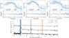Fig. 4.

X-ray and optical spectral properties of three X-ray obscured radio galaxies at z > 3 obtained by this study. Top: X-ray spectra of the three obscured radio galaxies at z > 3. All three sources are spec-z confirmed sources. The left panel is ERO_ID = 3682, z = 3.10, log(N_H/cm⁻²) = 22.1. The middle panel is ERO_ID = 3933, z = 3.09, log(N_H/cm⁻²) = 22.1. The right panel is ERO_ID = 7772, z = 3.11, log(N_H/cm⁻²) = 22.0. The best-fit model and its 99% confidence interval are displayed as blue shaded regions. For each source, the lower panel displays the ratio to the best-fit model. Bottom: optical spectra of the three obscured radio galaxies at z > 3. The spectra for ERO_ID = 3682 and 7772 are taken from the SDSS survey (Abdurro’uf et al. 2022) and the spectrum for ERO_ID = 3933 is taken from the WiggleZ survey, which uses AAT/AAOmega spectrograph (Drinkwater et al. 2018).

Since some of our samples also cover optical to mid-IR bands, a flux density ratio of f_ν(12 μm)/f_ν, i-band is calculated as an indicator of dust extinction (Ross et al. 2018). The observed WISE W3 (12 μm) flux density and Subaru/HSC i-band flux densities are used in this study. The bottom right panel of Fig. 3 shows the relation between the f_ν(12 μm)/f_ν, i-band and N_H, which are tracers of the dust extinction and the gas absorption, respectively. The scatter is huge, but the two parameters show a statistically significant correlation with each other, which is supported by Pearson’s test with a coefficient value of 0.34 and p-value of 7.2 × 10⁻⁷. The linear fitting result is also shown with the black dashed line, with the equation of log(f_ν(12 μm)/f_ν,i-band) = −14.1 + 0.73(N_H/cm⁻²).

The bottom right panel of Fig. 3 also shows the sources which fulfill the color criterion of extremely red quasars, which is defined as optically identified quasars with an observed flux density ratio of f_ν(12 μm)/f_ν, i-band > 10^1.84 (Ross et al. 2015; Hamann et al. 2017). Thanks to the deep photometries of Subaru/HSC, 16 out of the 23 sources have faint i_AB > 22, which is not covered by the previous studies (e.g., Ross et al. 2015). As shown in the figure, there is one spec-z source in the region of the extremely red quasar color. The source is ERO_ID = 608, which Brusa et al. (2022) already identified as an X-ray luminous obscured AGN with strong [OIII]λ5007 outflow feature, undergoing strong AGN feedback. This is consistent with one of the notable features of extremely red quasars (Zakamska et al. 2016). Although we must wait for further spectroscopic confirmation to know whether the other 22 sources of our candidates are genuinely extremely red quasars or not, our sample contains interesting candidates of such radio-loud extremely red quasars. Hwang et al. (2018) proposed that the origins of radio-emission for extremely red quasars would be a shocked induced emission by the strong outflows (e.g., Zakamska & Greene 2014) for the moderate radio luminosities of L_1.4 GHz/W Hz⁻¹ = 7 × 10²² − 10²⁵, where six of our extremely red quasar candidates fulfill this criterion. On the other hand, we also cover 17 radio luminous extremely red quasar candidates at 10²⁵ < (L_1.4 GHz/W Hz⁻¹) < 10^27.3, which might have not been investigated before.

3.3. X-ray and 6 μm luminosity correlation

It is not trivial to assume for radio AGN that the X-ray emission is dominated by the radiation from the corona around the accretion disk because of the possible contamination of the emission from the jet as shown in blazars (e.g., Ghisellini et al. 2017). To investigate this jet contribution in the X-ray bands we utilize the MIR bands, which are generally dominated by the thermal dust emission heated by the accretion disk of AGN, and investigate the luminosity relation between the X-ray and MIR band of our sample and compare it to the radio-quiet AGN, which show a tight correlation with each other in low-redshift (z < 0.1) and low-luminosity AGN at $L_{2 - 10 keV}^{(abs, corr)} < 10^{44}$ ${L_{2{-}10\,{\rm keV}}^{\rm (abs,corr)}} < 10^{44}$ erg s⁻¹ (Gandhi et al. 2009; Matsuta et al. 2012; Asmus et al. 2015; Ichikawa et al. 2012, 2017, 2019a) and also in high-redshift (z > 1) and high-luminosity AGN or quasars (Stern 2015; Mateos et al. 2015; Chen et al. 2017).

Figure 5 shows a luminosity correlation between the rest frame 6 μm (L_6 μm) and absorption corrected 2−10 keV band ( $L_{2 - 10 keV}^{(abs, corr)}$ ${L_{2{-}10\,{\rm keV}}^{\rm (abs,corr)}}$ ) extrapolated from the absorption corrected 0.5−2 keV luminosities ( $L_{0.5 - 2 keV}^{(abs, corr)}$ ${L_{0.5{-}2\,{\rm keV}}^{\rm (abs,corr)}}$ ). The reason why we use $L_{2 - 10 keV}^{(abs, corr)}$ ${L_{2{-}10\,{\rm keV}}^{\rm (abs,corr)}}$ here instead of $L_{0.5 - 2 keV}^{(abs, corr)}$ ${L_{0.5{-}2\,{\rm keV}}^{\rm (abs,corr)}}$ is for the comparison of the previous luminosity correlation studies that mostly utilize absorption corrected 2−10 keV luminosities (e.g., Stern 2015; Chen et al. 2017). Overall, most sources in our sample follow nicely the luminosity correlation of radio-quiet quasars of the similar redshift (Stern 2015; Chen et al. 2017), which shows a saturation of X-ray emission in the high-luminosity end. This trend is also consistent with the results of the obscured AGN sample in the eFEDS field (Toba et al. 2022). On the other hand, while the sample size is small, blazar populations are known to follow the 1:1 relation without showing the saturation of $L_{2 - 10 keV}^{(abs, corr)}$ ${L_{2{-}10\,{\rm keV}}^{\rm (abs,corr)}}$ (e.g., Matsuta et al. 2012). This indicates that both X-ray and 6 μm luminosity of our eFEDS-WERGS sample is dominated by the same radiation origins for radio-quiet populations and the contribution from the jet emission would be not a significant one on average.

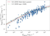Fig. 5.

Correlation between the luminosities at absorption corrected 2−10 keV ( $L_{2 - 10 keV}^{(abs, corr)}$ ${L_{2{-}10\,{\rm keV}}^{\rm (abs,corr)}}$ ) and 6 μm (L_6 μm). The symbols are the same as in Fig. 1. The red dashed and green dot-dashed line represents the slope in the study of optically selected radio-quiet quasars at 1.5 < z < 5 by Stern (2015) and Chen et al. (2017), respectively.

We also note that Fig. 5 shows a deviation of the sample from the slopes of Stern (2015) and Chen et al. (2017) at the low-luminosity end, notably at L_6 μm < 10⁴⁴ erg s⁻¹. This trend is discussed in Sect. 3.1.2 and Fig. 2, and the possible origins are the contamination from the host galaxies into the MIR bands where the AGN dust does not always outshine the host galaxy scale dust emission (Ichikawa et al. 2017). The other possibility is the contamination from the synchrotron radiation of the jet. Several low-luminosity AGN are known to show such synchrotron emission contamination even in the MIR bands (Mason et al. 2012; Privon et al. 2012; Lopez-Rodriguez et al. 2014, 2018). As we discuss in Sect. 6, these low-luminosity AGN tend to show high jet production efficiency, and therefore the relative contribution from the jet might be strong compared to the AGN dust emission. Nonetheless, in either case, our main conclusion does not change that the X-ray emission for the majority of the eFEDS-WERGS sample is likely dominated by the radiation from the corona, not by the jet.

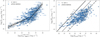Fig. 6.

Relation between the jet and accretion disk properties. Left: correlation between the luminosities at 1.4 GHz (L_1.4 GHz [erg s⁻¹]) and absorption corrected 2−10 keV ( $L_{2 - 10 keV}^{(abs, corr)}$ ${L_{2{-}10\,{\rm keV}}^{\rm (abs,corr)}}$ ). The two black dashed lines in the lower and higher $L_{2 - 10 keV}^{(abs, corr)}$ ${L_{2{-}10\,{\rm keV}}^{\rm (abs,corr)}}$ with the boundary of $L_{2 - 10 keV}^{(abs, corr)} = 10^{44}$ ${L_{2{-}10\,{\rm keV}}^{\rm (abs,corr)}} = 10^{44}$ erg s⁻¹ represent the fitting lines of Eqs. (3) and (4), respectively. Right: correlation between the jet power (P_jet) and bolometric AGN luminosity (L_AGN,bol). The black solid, dashed, and dot-dashed line shows the case with the jet production efficiency η_jet = 1, η_jet = 0.1, and η_jet = 0.01, respectively, by assuming the radiation efficiency of η_rad = 0.1 (Soltan 1982). The other symbols are the same as in Fig. 1.

3.4. Radio 1.4 GHz and X-ray luminosity correlation

The combination of the radio and X-ray data offers the opportunity to investigate the connection between the disk-corona (traced by X-rays) and the disk-jet (traced by radio wavelengths). The slope of the luminosity correlation between the radio and X-ray bands is thought to depend on the accretion disk properties. Several authors argue that the slope of L_R − L_X is different among the accretion disk states: at low accretion rates, radiatively inefficient accretion flow (RIAF; b ∼ 0.5 − 0.7; see Corbel et al. 2003; Gallo et al. 2003) and at high accretion rates, standard disk state (b ∼ 1.4; Coriat et al. 2012).

The left panel of Fig. 6 shows the luminosity correlation between rest-frame 1.4 GHz luminosity and absorption corrected 2−10 keV luminosity. While the scatter is large, there is a sign of the luminosity slope change at $log (L_{2 - 10 keV}^{(abs, corr)} / erg s^{- 1}) ≃ 44$ $\log ({L_{2{-}10\,{\rm keV}}^{\rm (abs,corr)}}/{\rm erg}\,{\rm s}^{-1})\simeq 44$ , below and above which the accretion state is likely the RIAF and standard disk state, respectively. This is partially supported by the fact that $log (L_{2 - 10 keV}^{(abs, corr)} / erg s^{- 1}) ≃ 44$ $\log ({L_{2{-}10\,{\rm keV}}^{\rm (abs,corr)}}/{\rm erg}\,{\rm s}^{-1})\simeq 4$ corresponds to log(L_AGN,bol/erg s⁻¹)≃45.7, which is the Eddington luminosity of the sources with log(M_BH/M_⊙) = 7.7, and therefore λ_Edd > 0.01 is the boundary for the sources with log(M_BH/M_⊙) < 9.7. In other words, most of the sources above the boundary $log (L_{2 - 10 keV}^{(abs, corr)} / erg s^{- 1}) ≃ 44$ $\log ({L_{2{-}10\,{\rm keV}}^{\rm (abs,corr)}}/{\rm erg}\,{\rm s}^{-1})\simeq 44$ should be in the efficient accretion phase of λ_Edd > 0.01.

We apply ordinary least-squares Bisector fits, which minimize the perpendicular distance from the slope line to data points (Schmitt 1985; Isobe et al. 1990). This gives the correlation at the low-luminosity end ( $L_{2 - 10 keV}^{(abs, corr)} < 10^{44}$ ${L_{2{-}10\,{\rm keV}}^{\rm (abs,corr)}}<10^{44}$ erg s⁻¹) with

$\begin{matrix} log \frac{L_{1.4 GHz}}{10^{41} erg s^{- 1}} = (0.38 \pm 0.08) + (0.69 \pm 0.07) log \frac{L_{2 - 10 keV}^{(abs, corr)}}{10^{44} erg s^{- 1}}, \end{matrix}$ $\begin{aligned} \log \frac{L_{\rm 1.4\,GHz}}{10^{41}\,\mathrm{erg}\,\mathrm{s}^{-1}} = (0.38 \pm 0.08) + (0.69 \pm 0.07) \log \frac{L_{2{-}10\,\mathrm{keV}}^\mathrm{(abs,corr)}}{10^{44}\,\mathrm{erg}\,\mathrm{s}^{-1}}, \end{aligned}$ (3)

and at the high-luminosity end ( $L_{2 - 10 keV}^{(abs, corr)} \geq 10^{44}$ ${L_{2{-}10\,{\rm keV}}^{\rm (abs,corr)}} \geq 10^{44}$ erg s⁻¹) with

$\begin{matrix} log \frac{L_{1.4 GHz}}{10^{41} erg s^{- 1}} = (- 0.07 \pm 0.10) + (1.73 \pm 0.12) log \frac{L_{2 - 10 keV}^{(abs, corr)}}{10^{44} erg s^{- 1}} \cdot \end{matrix}$ $\begin{aligned} \log \frac{L_{\rm 1.4\,GHz}}{10^{41}\,\mathrm{erg}\,\mathrm{s}^{-1}}= (-0.07 \pm 0.10) + (1.73 \pm 0.12) \log \frac{L_{2{-}10\,\mathrm{keV}}^\mathrm{(abs,corr)}}{10^{44}\,\mathrm{erg}\,\mathrm{s}^{-1}}\cdot \end{aligned}$ (4)

The obtained slope value of b = 0.69, which is defined by $log L_{1.4 GHz} \propto b log L_{2 - 10 keV}^{(abs,corr)}$ $\log {L_{\text{1.4\,GHz}}}\propto b \log {L_{2{-}10\,\text{ keV}}^{\text{(abs,corr)}}}$ , is consistent with those of RIAF for the low-luminosity end and the values expected from the fundamental planes (b ∼ 0.7, e.g., Merloni et al. 2003). On the other hand, the slope has a steeper value of b = 1.73 at the high $L_{2 - 10 keV}^{(abs, corr)}$ ${L_{2{-}10\,{\rm keV}}^{\rm (abs,corr)}}$ end. This high slope value is also reported in the ROSAT-FIRST radio quasar sample, which shows b = 2.1 (Brinkmann et al. 2000). This suggests that our sample contains radio jet efficient sources at the higher luminosity end, especially when X-ray emission saturates at $L_{2 - 10 keV}^{(abs, corr)} ≃ 10^{45 - 46}$ ${L_{2{-}10\,{\rm keV}}^{\rm (abs,corr)}}\simeq 10^{45{-}46}$ erg s⁻¹. Based on the results above, thanks to the broad coverage of $log (L_{2 - 10 keV}^{(abs, corr)} / erg s^{- 1}) = 41 - 46$ $\log ({L_{2{-}10\,{\rm keV}}^{\rm (abs,corr)}}/{\rm erg}\,{\rm s}^{-1}) = 41{-}46$ including both low- and high-accretion sources, we find an important trend: the luminosity correlation shows a break around $L_{2 - 10 keV}^{(abs, corr)} \sim 10^{44}$ ${L_{2{-}10\,{\rm keV}}^{\rm (abs,corr)}} \sim 10^{44}$ erg s⁻¹, above which $L_{2 - 10 keV}^{(abs, corr)}$ ${L_{2{-}10\,{\rm keV}}^{\rm (abs,corr)}}$ shows a saturation compared to L_1.4 GHz, which suggests that the X-ray corona and the radio–jet connection are fundamentally different below and above the break luminosity of $L_{2 - 10 keV}^{(abs, corr)} ≃ 10^{44}$ ${L_{2{-}10\,{\rm keV}}^{\rm (abs,corr)}}\simeq 10^{44}$ erg s⁻¹. We discuss this point in Sects. 3.5 and 3.7.

3.5. P_jet and L_AGN, bol relation

To investigate the jet and disk connection more quantitatively, we estimate the jet power and the bolometric AGN luminosities, both of which are the total power of the jet and radiation from the accretion disk. For the bolometric luminosity, we use the value estimated from $L_{2 - 10 keV}^{(abs, corr)}$ ${L_{2{-}10\,{\rm keV}}^{\rm (abs,corr)}}$ , as discussed in Sect. 2.4.1.

There are several studies measuring the relation between jet power and radio luminosities, and two approaches are commonly used. One is based on the analytic models of the sources to predict the radio luminosity for a given radio jet power (e.g., Willott et al. 1999). The other is based on the estimation of the jet power from the size of the X-ray cavities in the hot gas inflated by the radio lobes, and the X-ray cavity powers can be empirically related to the radio luminosity (e.g., Bîrzan et al. 2008; Cavagnolo et al. 2010). In this study, we use the relation based on the latter approach and the total jet power of the AGN (P_jet) is estimated from the VLA/FIRST radio luminosity. We adopt the relation between P_jet and L_1.4 GHz of Cavagnolo et al. (2010):

$\begin{matrix} P_{jet} = 1.05 \times 10^{44} {(L_{1.4 GHz} / 10^{24} W {Hz}^{- 1})}^{0.75} erg s^{- 1} . \end{matrix}$ $\begin{aligned} P_{\rm jet}= 1.05 \times 10^{44}\,(L_{\rm 1.4\,GHz}/10^{24}\,\mathrm{W\,Hz^{-1}})^{0.75}\,\mathrm{erg}\,\mathrm{s}^{-1}. \end{aligned}$ (5)

The results based on other relations are discussed in Appendix A. We note that the jet power is known to depend not only on the observed radio luminosity, but also on its radio source size, which is a rough indicator of the source age (called the power-linear size plane or P_jet − D diagram; e.g., Baldwin 1982; Kaiser et al. 1997; Blundell et al. 1999; An & Baan 2012), and its redshift due to the Compton loss at higher-z at z ≥ 2 (e.g., Hardcastle 2018; Hardcastle et al. 2019). Shabala & Godfrey (2013) recently investigated the effect of the radio source size in the jet power estimation, and found the dependence on the source size to be ∝D^0.58, suggesting that the effect of the source size is small. Since our sample is selected only for radio-compact emission in VLA/FIRST with a spatial resolution of ∼5 arcsec (or ≲20 kpc at z ∼ 1), this again mitigates the size dependence; otherwise the sources are ultra-compact sources. We discuss the redshift dependence below.

The left panel of Fig. 7 shows the distribution of P_jet, spanning wide luminosity range of 43.2 < log(P_jet/erg s⁻¹) < 47.4. In particular, the high P_jet sources with log(P_jet/erg s⁻¹) > 45.0 is almost equivalent to the radio-loud quasar level (e.g., Best et al. 2005; Inoue et al. 2017). The eFEDS-WERGS sample covers high P_jet sources, which are powerful enough to produce an expanding jet with ≳10 kpc that can disrupt the interstellar medium (e.g., Nesvadba et al. 2017) and larger scale intergalactic environments, possibly quenching star formation in host galaxies (e.g., McNamara & Nulsen 2007).

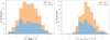Fig. 7.

Distribution of P_jet/erg s⁻¹ (left) and η_jet assuming the radiative efficiency of 0.1 (right). The sample is divided into subgroups of spec-z sources (cyan) and photo-z sources (orange).

The right panel of Fig. 6 shows the relation between the jet power P_jet and the bolometric AGN luminosity L_AGN,bol. As expected from the correlation between L_1.4 GHz and $L_{2 - 10 keV}^{(abs, corr)}$ ${L_{2{-}10\,{\rm keV}}^{\rm (abs,corr)}}$ , the relation shows a flatter trend in the low L_AGN,bol and the slope becomes steeper at higher L_AGN,bol, notably at L_AGN,bol > 10^45.5 erg s⁻¹, which shows a slope value of b ≈ 1.0. The slope is shallower than b = 1.73 in Eq. (4) because of the X-ray luminosity-dependent bolometric correction by Marconi et al. (2004). This 1:1 slope is consistent with the value previously reported in the SDSS radio quasars by using optical and UV continuum as an indicator of AGN radiation (e.g., Inoue et al. 2017).

Considering that jet production is correlated to the accretion rate to the BH Ṁ_BH, the jet power is limited by the BH accretion rate with a jet production efficiency. The jet production efficiency is defined as

$\begin{matrix} η_{jet} = P_{jet} / {\dot{M}}_{BH} c^{2} = η_{rad} P_{jet} / L_{AGN, bol}, \end{matrix}$ $\begin{aligned} \eta _{\rm jet}= P_{\rm jet}/\dot{M}_{\rm BH}c^2 = \eta _{\rm rad}P_{\rm jet}/L_{\rm AGN,bol}, \end{aligned}$ (6)

where η_rad is the radiation efficiency of an AGN accretion disk, c is the speed of light, and Ṁ_BH is the mass accretion rate onto the SMBH through the disk. In the following we adopt a canonical value of η_rad = 0.1 based on the Soltan–Paczynski argument (Soltan 1982). The solid line in the right panel of Fig. 6 represents P_jet = L_AGN,bol/η_rad = Ṁ_BHc², corresponding to the maximum efficiency of η_jet = 1, and the dashed and dot-dashed line represents the value with η_jet = 0.1 and η_jet = 0.01.

The median value of η_jet is ⟨log η_jet⟩= − 1.0 ± 0.6 for the sources with L_AGN,bol < 10⁴⁵ erg s⁻¹ and ⟨log η_jet⟩= − 2.0 ± 0.7 for high-luminosity sources with L_AGN,bol > 10⁴⁵ erg s⁻¹, respectively. The overall distribution is summarized in the right panel of Fig. 7. At the high-luminosity end, the jet production efficiency is almost consistent with the studies of the SDSS radio quasar population, whose radio jet efficiency lies at ⟨log η_jet⟩= − 2.0 ± 0.5 (e.g., van Velzen & Falcke 2013; Inoue et al. 2017). The origin of the jet emission for those high-luminosity sources is still unclear since they would host standard geometrically thin disks, which are not expected to have powerful jets (Lubow et al. 1994). However, recent general relativistic magnetohydrodynamic (GR-MHD) simulations succeed in reproducing the jet launching even in such geometrically thin disks (e.g., Liska et al. 2019). Finally, we note that our estimation of η_jet might be underestimated for such high-luminosity sources with L_AGN,bol > 10⁴⁵ erg s⁻¹, whose median redshift is ⟨z⟩ = 1.3. Hardcastle (2018) discussed that the observed radio luminosities in high-z sources tend to show lower values for a given P_jet because of the increased inverse-Compton losses due to the increased CMB backgrounds with redshift. At z ∼ 2 the luminosity loss reaches a factor of a few at the jet age of a few Myr, and its radio size is around a few 10 kpc (Hardcastle 2018), which is the maximum end of the size in our VLA/FIRST radio compact sources. Thus, a possible underestimation of η_jet could reach a factor of a few. Nonetheless, this difference does not affect our main conclusion here.

At the low-luminosity end, the jet production efficiency is slightly higher or consistent with the nearby radio AGN population (log η_jet ∼ −1.5) whose host galaxies are massive (M_⋆ > 10¹¹ M_⊙; Nemmen & Tchekhovskoy 2015). One notable trend, especially at the low AGN luminosity end, is that some low-luminosity sources reach extremely high jet production efficiency at η_jet ∼ 1 (14 sources fulfill the criteria of η_jet + Δη_jet > 1). This extremely high value can be achieved if the sources are blazars with extremely high BH spin value (e.g., Ghisellini et al. 2014). However, most of such high η_jet sources are spec-z confirmed sources and they are categorized as non-blazars. Therefore, it is unlikely that blazars are the majority of the population.

The second possibility is that our assumption of η_rad = 0.1 is no longer valid in the low-luminosity AGN regime at λ_Edd < 0.01. At sufficiently low accretion rates, the infalling matter to the BH is not dense enough to cool any longer, deviating from the standard-disk model. Thus, the flow is essentially adiabatic and mass accretion is led by anomalous viscosity produced by the magneto-rotational instability (e.g., Balbus & Hawley 1991). There are several accretion disk models in such low-accretion regimes, and the radiation efficiency differs among them. One RIAF model (Ichimaru 1977; Narayan & Yi 1994, 1995; Stone & Pringle 2001; Hawley & Balbus 2002) predicts that η_rad ∼ 10⁻² and η_rad ∼ 10⁻³ at λ_Edd ∼ 10⁻² and λ_Edd ∼ 10⁻³, respectively (Ciotti et al. 2009; Xie & Yuan 2012; Inayoshi et al. 2019). On the other hand, several authors have shown that rotating accretion flows become convectively unstable and become convection-dominated accretion flows (Igumenshchev & Abramowicz 1999; Stone et al. 1999; Narayan et al. 2000), which shows higher η_rad than the other RIAF models, with η_rad ∼ 10⁻² and η_rad ∼ 10⁻³ at λ_Edd ∼ 10⁻⁴ and λ_Edd ∼ 10⁻⁶, respectively (Xie & Yuan 2012; Ryan et al. 2017; Inayoshi et al. 2019). As we discuss in Sect. 3.6, the expected λ_Edd range is −4 < log λ_Edd < −2, and therefore η_rad = 10⁻³ to 10⁻² for both models, resulting in η_jet being reduced from η_jet ∼ 1 into lower values with η_jet ∼ 10⁻¹ to ∼10⁻².

The third possibility is that sources show high η_jet because the central engine is experiencing a quenching of AGN activity. It is known that jet emission is quite stable over the timescale of ∼10 Myr even after the energy injection stops from the central engine (e.g., Kaiser et al. 1997; Shabala et al. 2020; Jurlin et al. 2021; Morganti et al. 2021), indicating that the jet luminosity does not fade drastically on this timescale. We note that the main discussions in the references were based on the 140 MHz band, but the spectral aging method shows that the trend does not change drastically even at 1.4 GHz on a timescale of < 10 Myr (e.g., Harwood et al. 2013). On the other hand, L_AGN,bol in this study is estimated from the X-ray observation. This emission can be used as the indicator of the current AGN luminosities (e.g., Ichikawa et al. 2019b) since it originates from the X-ray corona on the physical scale of approximately ten gravitational radii (e.g., Morgan et al. 2010). Once the galaxies experience the AGN feedback and prompt gas feeding to the BH decreases within a ∼10 Myr timescale, we can witness a decrease in $L_{0.5 - 2 keV}^{(abs, corr)}$ ${L_{0.5{-}2\,{\rm keV}}^{\rm (abs,corr)}}$ , and therefore a decrease in L_AGN,bol, while L_1.4 GHz remains stable. This different response time of the two luminosities might increase η_jet higher, sometimes reaching nearly the maximum limit of η_jet, and it also goes even higher than the limit of η_jet = 1, as shown in the right panel of Fig. 6. For the sources at η_jet ∼ 1, considering that the average η_jet is higher by one order of magnitude compared to typical radio galaxies, and two orders of magnitude higher than the typical radio-loud quasars, the central engine might have experienced a drastic luminosity decline by a factor of ∼10−100 within the constant jet regime (i.e., on the order of ∼10 Myr).

Some might wonder how likely such a drastic AGN luminosity decline could happen. Actually, recent multiwavelength observations have enabled us to probe different AGN signatures with different physical scales covering up to ∼10 kpc, and they have discovered an AGN population with drastic luminosity declines by a factor of 10 − 10³ in the last 10^4 − 5 yr. They are called fading AGN and nearly 100 sources have been reported so far (Schawinski et al. 2010; Keel et al. 2015, 2017; Ichikawa et al. 2016, 2019a,b; Schirmer et al. 2016; Sartori et al. 2018; Villar-Martín et al. 2018; Wylezalek et al. 2018; Chen et al. 2020; Pflugradt et al. 2022; Saade et al. 2022; Finlez et al. 2022), and some of the sources with η_jet ∼ 1 might be one of them. In order to judge whether they are such fading AGN populations, additional multiwavelength information is necessary to obtain the AGN signature tracing the physical scale difference, and therefore the probes of AGN luminosities (such as [OIII]λ5007 emissions as a tracer of an extended narrow line region) in the past 10^3 − 4 yr (e.g., Keel et al. 2017; Ichikawa et al. 2019a).

3.6. SMBH properties: Relation between sBHAR and M_⋆

Considering that some eFEDS-WERGS are faint in the optical, as shown in Fig. 1, sometimes it is difficult to obtain the BH mass through optical spectroscopy (but see Merloni et al., in prep.). In addition, direct BH mass estimation is not available for optically type 2 AGN, although several indirect BH mass estimations are presented (e.g., Baron & Ménard 2019). Instead, we investigate the SMBH properties through the specific black hole accretion rate (sBHAR), which is considered to be a good proxy for the Eddington ratio. The sBHAR is conventionally defined as sBHAR = L_AGN,bol/M_⋆ erg s $^{- 1} M_{⊙}^{- 1}$ $^{-1}\,M_{\odot}^{-1}$ (Aird et al. 2012, 2019; Mullaney et al. 2012; Delvecchio et al. 2018), and the relation between the sBHAR and the Eddginton ratio λ_Edd is summarized by Ichikawa et al. (2021); it can be written as a function of λ_Edd and M_⋆ as

$\begin{matrix} sBHAR = 4.6 \times 10^{35} λ_{Edd} {(M_{⋆} / 10^{10} M_{⊙})}^{0.4} . \end{matrix}$ $\begin{aligned} \mathrm{sBHAR} = 4.6\times 10^{35} \lambda _{\rm Edd} \left(M_{\star }/10^{10}\,M_{\odot }\right)^{0.4}. \end{aligned}$ (7)

Here we apply stellar-mass dependent values for M_BH with $M_{BH} \propto M_{⋆}^{β}$ ${M_{\rm BH}} \propto M_\star^\beta$ , where β = 1.4 (Kormendy & Ho 2013) and M_⋆ is available at 0 < z < 1 through the image decomposition of HSC optical images of the targets.

Figure 8 shows sBHAR as a function of M_⋆ for eFEDS-WERGS sources at z < 1. This shows that 58% of eFEDS-WERGS sources (81 out of 139 sources) are above the line of λ_Edd = 0.01 (black dashed line), indicating that roughly half of them are highly gas accreting sources even though they are radio bright. In particular, a fraction of sources are located at the vicinity of the Eddington limit of λ_Edd = 1. On the other hand, the remaining 42% of the population (58 sources) are below the line of λ_Edd = 0.01 and are clustered at 10⁻⁴ < λ_Edd < 0.01. While the sample in Fig. 8 is limited for the sources at z < 1, which misses a large population of high-luminosity sources, this trend is consistent with the result in Fig. 6, which shows a steep slope trend at the high-luminosity end, indicating these sources are in a standard disk state or even the slim disk state, while the low-luminosity sources are in a radiatively inefficient state.

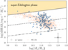Fig. 8.

Relation between sBHAR (=L_AGN,bol/M_⋆ erg s $^{- 1} M_{⊙}^{- 1}$ $^{-1}\,M_{\odot}^{-1}$ ) and M_⋆. The gray cross represents the typical error bar of the two values. The orange shaded area represents the region of super-Eddington λ_Edd > 1. The three straight lines (from top to bottom) are the expected Eddington ratio of λ_Edd = 1 (Eddington limit; black solid line), λ_Edd = 0.01 (black dashed line), and λ_Edd = 10⁻⁴ (black dot-dashed line) using Eq. (7). The pale pink stars in the background represent the sources from the original WERGS sample with IR detections (KI+21; Ichikawa et al. 2021). The other symbols are the same as in Fig. 1.

The background red points are WERGS radio galaxies at 0.3 < z < 1.6 obtained from Ichikawa et al. (2021), which covers optically very faint sources down to i_AB ∼ 26. Their AGN luminosities and stellar masses are obtained from the SED fitting using CIGALE to the photometric data from the optical to mid-IR bands. Thanks to the deep optical photometries and wide coverage of wavelength bands which enable them to cover low stellar-mass regimes down to log(M_⋆/M_⊙)≃9.5. On the other hand, our eFEDS-WERGS sample is biased to relatively bright sources with i_AB < 23, and only for the reliable stellar-mass measurements from Li et al. (2021), which produces a clear stellar-mass cut at M_⋆ > 10^10.5 M_⊙. Once more multiwavelength information is assembled, the expansion of the sample into higher redshift and lower stellar mass might uncover more high sBHAR sources.

3.7. Fundamental plane of eFEDS-WERGS AGN

The fundamental plane of BH activity is the relation among three parameters of M_BH, L_R, and L_X, where L_R = νL_ν(5 GHz), L_X = L_{2 − 10 keV}. The empirical relation of the fundamental plane has been reported since the late 1990s (Hannikainen et al. 1998), and this relation gives the important observational connection related to accretion-jet phenomena. The studies of fundamental planes are mainly focused on the low accretion rate phase, such as the RIAF state with < 0.01Ṁ_BH, where the radiation from a BH is non-thermally dominated (e.g., Merloni et al. 2003; Heinz & Sunyaev 2003; Falcke et al. 2004). On the other hand, at the phase of high accretion rate, the radiation is more thermally dominated, and it is of great importance whether the universal trend of the fundamental plane is maintained, even including the luminous radio galaxies, such as our sample. If so, the fundamental plane hosts the powerful ability to use radio and X-ray observations to estimate black hole mass, which would be a good alternative method where other methods are not available.

Since both of the nuclear radio and X-ray luminosities are already obtained in this study, we estimate the BH from the fundamental plane relation by adapting the studies of Gültekin et al. (2019), which is written as

$\begin{matrix} log (M_{BH, FP} / 10^{8} M_{⊙}) = & μ_{0} + ξ_{5 GHz} log (L_{5 GHz} / 10^{38} erg s^{- 1}) \\ + ξ_{2 - 10 keV} log (L_{2 - 10 keV} / 10^{40} erg s^{- 1}), \end{matrix}$ $\begin{aligned} \log (M_{\rm BH,FP}/10^8\,M_\odot ) =&\mu _0 + \xi _{\rm 5\,GHz} \log (L_{\rm 5\,GHz}/10^{38}\,\mathrm{erg\,s^{-1}})\nonumber \\&+ \xi _{\rm 2{-}10\,keV} \log (L_{\rm 2{-}10\,keV}/10^{40}\,\mathrm{erg\,s^{-1}}), \end{aligned}$ (8)

where μ₀ = 0.55 ± 0.22, ξ_5 GHz = 1.09 ± 0.10, and ξ_{2 − 10 keV} = −0.59 ± 0.16. We note that this relation is based on the sample of X-ray binaries and AGN whose Eddington ratios are mostly λ_Edd < 0.01. The 5 GHz radio luminosity (L_5 GHz) is extrapolated from L_1.4 GHz by assuming the power-law radio spectrum with f_ν ∝ ν^α and α = −0.7.

Figure 9 shows the BH masses estimated from the fundamental plane (M_BH,FP) as a function of redshift. Some of the obtained M_BH,FP values exceed the observationally known maximum BH mass limit of M_BH,FP > 10^10.5 M_⊙ across the Universe at 0 < z < 7.5 (McConnell et al. 2011; Kormendy & Ho 2013; Trakhtenbrot 2014; Jun et al. 2015; Wu et al. 2015; Bañados et al. 2018; Yang et al. 2020). This suggests that M_BH,FP is significantly overestimated, sometimes by one to three orders of magnitude. This huge discrepancy is well beyond the intrinsically large scatter of the original fundamental plane of σ ≈ 0.8 dex.

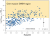Fig. 9.

Black hole mass estimated from the fundamental plane as a function of redshift. The orange shaded area represents the over-massive SMBH region above the maximum mass limit of known SMBHs (e.g., Kormendy & Ho 2013).

To investigate this point, we compare the obtained M_BH,FP with the BH masses estimated from the stellar mass (M_BH, ⋆) estimated from the 2D image decomposition at z < 1. Here we apply the M_BH − M_⋆ relation in the local universe (Kormendy & Ho 2013). The top left panel of Fig. 10 shows the relation between the two BH mass estimates of M_BH,FP and M_BH, ⋆. The obtained M_BH, ⋆ is in the range of the known SMBH mass range of M_BH < 10^10.5 M_⊙. While 78 out of the 139 sources are within the scatter of σ ≈ 0.8 dex between the two BH mass values, two BH mass values do not follow the expected 1:1 relation for the remaining 61 sources, but rather show a clear excess in M_BH,FP/M_BH, ⋆. The result above indicates that our eFEDS-WERGS sources do not follow the fundamental plane for some sources. This might be a natural outcome considering that most of the fundamental plane is based on the low-accreting black holes, while roughly half of our sources are likely highly accreting sources, as shown in Sect. 3.6.

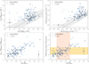Fig. 10.

Relations between the values obtained from the BH fundamental plane and those obtained in this study. Top left: relation between two different BH mass estimations. M_BH,FP is obtained from the fundamental plane of Gültekin et al. (2019) and by using the obtained X-ray and radio luminosities in this study. M_BH, ⋆ is the BH mass estimated from the scaling relation of Kormendy & Ho (2013) and by using the obtained stellar mass. The gray cross represents the typical error bar of the two parameters. The gray dashed line represents the 1:1 line with the scatter area of the typical error bar. Top right: relation between the L_{5 GHz, FIRST} and L_{5 GHz, FP}, which is estimated from the fundamental plane relation of Gültekin et al. (2019) with the values of M_BH, ⋆ and $L_{2 - 10 keV}^{(abs, corr)}$ ${L_{2{-}10\,{\rm keV}}^{\rm (abs,corr)}}$ . The gray cross represents the typical error bar of the two parameters. The gray dashed line represents the 1:1 line, with the scatter area of the typical error bar. Bottom left: black hole mass ratio of M_BH,FP/M_BH, ⋆ as a function of ℛ_obs. Bottom right: radio-luminosity ratio of L_{5 GHz, FIRST}/L_{5 GHz, FP} as a function of ℛ_obs. The orange shaded area represents the possible Doppler boost area by assuming typical radio-loud AGN. The red shaded area represents the possible range of the ℛ_obs for blazars by assuming a blazar sequence at 0 < z < 5. The gray cross represents the typical error bar of the two values in each panel.

The top right panel of Fig. 10 shows the relation between the L_{5 GHz, FIRST} and the estimated 5 GHz radio luminosity from the fundamental plane by using the obtained M_BH, ⋆ and $L_{2 - 10 keV}^{(abs, corr)}$ ${L_{2{-}10\,{\rm keV}}^{\rm (abs,corr)}}$ (L_{5 GHz, FP}). This shows that our eFEDS-WERGS shows a strong radio emission excess compared to the expected value from the fundamental plane. The obtained radio emission excess ranges up to three orders of magnitude, and cannot be solely explained by differences in the radio slope α (where f_ν ∝ ν^α), which only results in a 0.2 dex difference for −1.0 < α < −0.5, as demonstrated by the typical error bar in the panel, and at most a 0.5 dex difference even for the steepest value of α = −1.7.

The bottom left panel of Fig. 10 shows a relation between the ratio of M_BH,FP/M_BH, ⋆ as a function of the observed radio loudness (ℛ_obs). The figure shows a good linear relation between the two values, supporting that radio-emission excess compared to the optical radiation produces the excess in the M_BH,FP estimation.

One possible origin of such radio emission excess might be from the beaming effect of the jet emission in the radio band (Wang et al. 2006; Li et al. 2008; Dong & Wu 2015). Li et al. (2008) discussed how much the boosting factor can produce the observed excess of the radio emission as a function of the Lorentz factor (Γ_L) and the inclination angle θ, where θ = 0 means face-on view (see also the discussion in Heinz & Merloni 2004). They demonstrate that radio emission excess is estimated to be less than 30 for most of the cases by assuming the typical Lorentz factor of Γ_L = 5 (Orr & Browne 1982) and an expected inclination angle of θ > 10° (Maraschi & Rovetti 1994). The bottom right panel of Fig. 10 shows the radio luminosity ratio of L_{5 GHz, FIRST}/L_{5 GHz, FP} as a function of ℛ_obs. The orange shaded region is the expected range of the radio emission excess for typical radio-loud AGN and quasars, as discussed above. Some of the sources with log ℛ_obs < 3 are in this range, suggesting that radio emission excess might be a boost origin. On the other hand, for the sources with log ℛ_obs > 3, the radio emission excess cannot be explained with the Lorentz boost alone, with a typical Lorentz factor and the inclination angle.

Li et al. (2008) also demonstrated that radio emission can boost at maximum of L_{5 GHz, FIRST}/L_{5 GHz, FP} ≲ 10³ assuming the extreme case with Γ_L > 10 and θ ≪ 10°, which would be achievable for blazar cases. On the other hand, Ichikawa et al. (2021) discussed the possible ℛ_obs range for blazars based on the known blazar sequence in the radio and optical bands (Fossati et al. 1998; Donato et al. 2001; Inoue & Totani 2009; Ghisellini et al. 2017). The observed radio loudness of blazars is in the range of log ℛ_obs ∼ 1.5 − 3. This range is obtained by using the luminosity range of L_1.4 GHz = 10⁴¹⁻⁴³ erg s⁻¹ and shifting redshift to the range of z ∼ 0 − 5. This area is shown as a pink colored area in the bottom panel of Fig. 10. The combination shows that although some of our eFEDS-WERGS sources might have a boosted radio emission in the FIRST band, there are still sources whose radio emission excess cannot be explained by the Lorentz boost alone. This is more prominent if sources have high radio loudness of log ℛ_obs > 3.

The additional origins of strong radio emission for those sources with log ℛ_obs > 3 is unclear, but one key aspect is that most of them are likely highly accreting sources. Such high jet emission efficiency can be achieved if the accretion disk of such sources is actually in the “radiatively inefficient” state, but the physical origin of radiative inefficiency is different from the disks in the local radio galaxies. They may be undergoing more rapid mass accretion (known as the Slim disk model; Abramowicz et al. 1988). Recent radiation hydrodynamical simulations suggest that when the mass accretion rate significantly exceeds the Eddington rate, radiation is effectively trapped within the accreting matter and advected to the central BH before escaping by radiative diffusion. As a result, the emergent radiation luminosity is saturated on the order of L_Edd (i.e., η_rad ≲ 0.1 at ≫ Ṁ_Edd) and the accretion flow turns into a radiatively inefficient state even with a super-Eddington accretion rate (e.g., Ohsuga et al. 2005, 2009; McKinney et al. 2014; Inayoshi et al. 2016; Takeo et al. 2020).

This would produce the suppressed X-ray emission and more prominent radio emission, which produces a larger discrepancy between the L_{5 GHz, FIRST} and L_{5 GHz, FP} and leads to higher L_{5 GHz, FIRST}/L_{5 GHz, FP}. This is prominent in Fig. 11, which shows the eFEDS-WERGS sources in the plane of L_{5 GHz, FIRST}/L_{5 GHz, FP} and sBHAR. While the sample size is limited at z < 1 because of the availability of M_⋆ in this study, the sources with high sBHAR, and around the expected Eddington limit region (yellow shaded area) might have a tentative sign of an excess of L_{5 GHz, FIRST}/L_{5 GHz, FP}. However, this trend should be confirmed by obtaining the stellar mass or BH masses of our high-z (z > 1) eFEDS-WERGS sample, which would contain more Eddington-limit sources rather than the sources discussed here at z < 1. This phase is considered to be a key process of the BH seed growth in the high-z (z > 6) universe to describe the already-known massive high-z SMBHs (e.g., Mortlock et al. 2011; Wu et al. 2015; Bañados et al. 2018; Onoue et al. 2019) and such high radio-loudness sources with log ℛ_obs > 3 would be prominent candidates for such a high accreting phase.

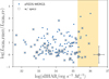Fig. 11.

Radio-luminosity ratio of L_{5 GHz, FIRST}/L_{5 GHz, FP} as a function of sBHAR. The yellow shaded area represents the corresponding Eddington limit accretion (λ_Edd = 1) region assuming the local scaling relation of M_BH − M_⋆ (Kormendy & Ho 2013) for the range of 9 < log(M_⋆/M_⊙) < 12 where our sources reside, as shown in Fig. 8. The gray cross represents the typical error bar of the two values.

4. Conclusion

The Subaru/HSC SSP survey enables us to find optical counterparts missed in the previous surveys. The WERGS catalog (Yamashita et al. 2018) provides the widest (> 100 deg²) and deepest (i_AB ∼ 26) optical counterparts of the radio bright VLA/FIRST population whose optical counterparts were missing before. We constructed the first X-ray catalog of WERGS radio galaxies in the 140 deg² eFEDS field. Thanks to the wide and medium-depth X-ray survey down to f_{0.5 − 2 keV} = 6.5 × 10⁻¹⁵ erg s cm⁻² by eROSITA on board the Spektrum-Roentgen-Gamma (SRG) mission in the eFEDS field, we found 393 (180 spec-z and 213 reliable photo-z) eROSITA detected WERGS radio galaxies (the eFEDS-WERGS catalog) spanning the wide redshift range at 0 < z < 6, where most of them reside in 0 < z < 4. By combining with the eFEDS X-ray catalog by Liu et al. (2022) and the multiwavelength catalog by Salvato et al. (2022), the eFEDS-WERGS catalog contains a wealth of information crucial for both of BHs and the host galaxies, including X-ray, radio, and mid-infrared luminosities and the column density N_H, as well as the host galaxy properties such as stellar mass for the 139 sources at z < 1 thanks to the high spatial resolution imaging by Subaru/HSC (Li et al. 2021).

We investigated the properties of the eFEDS-WERGS radio galaxies and found the following key results:

Thanks to the wide and medium depth X-ray surveys, eFEDS-WERGS catalog contains the rare and the most X-ray and mid-IR luminous radio galaxies above the knee of the X-ray luminosity function at 1 < z < 4, spanning $44 < (L_{0.5 - 2 keV}^{(abs, corr)} / erg s^{- 1}) < 46.5$ $44 < ({L_{0.5{-}2\,{\rm keV}}^{\rm (abs,corr)}}/{\rm erg}\,{\rm s}^{-1}) < 46.5$ and/or 45 < (L_12 μm/erg s⁻¹) < 47. The sample also covers the sources around and below the knee for the sources at z < 1.
A total of 91% of the sample (356 out of 393 sources) are unobscured AGN with log(N_H/cm⁻²) < 22, while the rare 9% of the sample (37 sources) show obscured AGN signatures with log(N_H/cm⁻²) > 22. Most of these obscured AGN are relatively high-z (0.4 < z < 3.2), and they are X-ray luminous with $(L_{0.5 - 2 keV}^{(abs, corr)} / erg s^{- 1}) > 44$ $({L_{0.5{-}2\,{\rm keV}}^{\rm (abs,corr)}}/{\rm erg}\,{\rm s}^{-1})>44$ , which is similar to luminosities with the SDSS optical quasars. Thus, they are obscured counterparts of the radio-loud quasars, which were largely missed in the previous studies, and are one of the important populations to study the quasar evolution at z = 1 − 3.
The majority of the eFEDS-WERGS sources follow the almost similar luminosity correlations of $L_{2 - 10 keV}^{(abs, corr)} - L_{6 μ m}$ ${L_{2{-}10\,{\rm keV}}^{\rm (abs,corr)}}{-}{L_{6\,\muup{\rm m}}}$ of radio-quiet AGN and quasars. This indicates that the X-ray and mid-IR bands trace the AGN corona and dust emissions, respectively, without contamination by the jet emission, even for radio galaxies, and the majority of the eFEDS-WERGS are likely to be non-blazars.
The $L_{1.4 GHz} - L_{2 - 10 keV}^{(abs,corr)}$ ${L_{\text{1.4\,GHz}}}{-}{L_{2{-}10\,\text{ keV}}^{\text{(abs,corr)}}}$ relation shows a different slope trend between the low- and high-luminosity end with the boundary of $(L_{2 - 10 keV}^{(abs, corr)} / erg s^{- 1}) \sim 44$ $({L_{2{-}10\,{\rm keV}}^{\rm (abs,corr)}}/{\rm erg}\,{\rm s}^{-1})\sim44$ . P_jet − L_AGN,bol relation revealed that there are sources with high jet production efficiency at η_jet ≈ 1. Such a high η_jet originates either from the lower radiative efficiency for those low-luminosity AGN or from the result of the experienced AGN feedback by jet within ∼Myr, which produces the declining of L_AGN,bol by a factor of 10−100 by keeping P_jet constant in the previous Myr, leading the boost of the obtained η_jet.
The expected BH mass (M_BH,FP) estimated from the fundamental plane and L_5 GHz and $L_{2 - 10 keV}^{(abs, corr)}$ ${L_{2{-}10\,{\rm keV}}^{\rm (abs,corr)}}$ obtained by the eFEDS-WERGS sources show unreasonably high values at M_BH,FP > 10¹⁰ M_⊙ for some sources, indicating that eFEDS-WERGS show a deviation from the conventional fundamental plane relation. This deviation stems from high ℛ_obs, the excess of radio luminosities. Such radio emission excess cannot be explained by the Doppler boosting alone, and therefore the disk-jet connection for some sources of the eFEDS-WERGS sample might be fundamentally different from the conventional plane that mainly traces the low accretion rate based sources.

¹

In general, the term “radio galaxies” represents the edge-on view (type 2) radio AGN whose host galaxies are detectable in the optical band (Antonucci 1993; Urry & Padovani 1995). In this study we use the term radio galaxies as AGN with significant radio detection, and therefore radio galaxies in this study are not necessarily type 2 AGN. For more details, see Sect. 2.3.

²

The optical counterpart fraction reaches ∼95% if the sample is limited to FIRST compact sources, where the cases of lobe contamination become negligible (Yamashita et al. 2018).

³

In the eFEDS field there are N_eFEDS = 17 603 circles with the area of S = πR² arcsec², where R = 1 arcsec. The surface number density of the FIRST sources in the eFEDS field (140 deg²) is Ω_FIRST = N_FIRST/(140 × 3600 × 3600) = 6.8 × 10⁻⁶ counts arcsec⁻² by using N_FIRST = 12 375. The expected coincident matching in the eFEDS is n = N_eFEDS × S × Ω_FIRST = 0.37.

⁴

There are two sources at z > 4, but are not shown in Fig. 2 for the illustrative purpose. Both are photo-z sources, but each shows a clear g-dropout (z = 4.2) and r-dropout feature (z = 5.4).

Acknowledgments

We appreciate the referee for the constructive and fruitful comments which deepen our understanding of the sample. We thank Yoshiyuki Inoue for providing us with the blazar sequence SED templates. This work is supported by Program for Establishing a Consortium for the Development of Human Resources in Science and Technology, Japan Science and Technology Agency (JST) and is partially supported by Japan Society for the Promotion of Science (JSPS) KAKENHI (20H01939; K. Ichikawa, T. Kawamruo; JP20K14529). K. Ichikawa also thanks Max Planck Institute for hosting me and most of the studies are conducted at MPE. K.I. acknowledges support from the National Natural Science Foundation of China (12073003, 12003003, 11721303, 11991052, 11950410493). T.K. acknowledges support from FONDECYT Postdoctral Fellowship (3200470). This work is based on data from eROSITA, the soft X-ray instrument aboard SRG, a joint Russian-German science mission supported by the Russian Space Agency (Roskosmos), in the interests of the Russian Academy of Sciences represented by its Space Research Institute (IKI), and the Deutsches Zentrum für Luft- und Raumfahrt (DLR). The SRG spacecraft was built by Lavochkin Association (NPOL) and its subcontractors, and is operated by NPOL with support from the Max Planck Institute for Extraterrestrial Physics (MPE). The development and construction of the eROSITA X-ray instrument was led by MPE, with contributions from the Dr. Karl Remeis Observatory Bamberg & ECAP (FAU Erlangen-Nuernberg), the University of Hamburg Observatory, the Leibniz Institute for Astrophysics Potsdam (AIP), and the Institute for Astronomy and Astrophysics of the University of Tübingen, with the support of DLR and the Max Planck Society. The Argelander Institute for Astronomy of the University of Bonn and the Ludwig Maximilians Universität Munich also participated in the science preparation for eROSITA. The Hyper Suprime-Cam (HSC) Collaboration includes the astronomical communities of Japan and Taiwan, and Princeton University. The HSC instrumentation and software were developed by the National Astronomical Observatory of Japan(NAOJ), the Kavli Institute for the Physics and Mathematics of the Universe (Kavli IPMU), the University of Tokyo, the High Energy Accelerator Research Organization (KEK), the Academia Sinica Institute for Astronomy and Astrophysics in Taiwan (ASIAA), and Princeton University. Funding was contributed by the FIRST program from Japanese Cabinet Office, the Ministry of Education, Culture, Sports, Science and Technology (MEXT), the Japan Society for the Promotion of Science (JSPS), Japan Science and Technology Agency (JST), the Toray Science Foundation, NAOJ, Kavli IPMU, KEK, ASIAA, and Princeton University. Funding for the Sloan Digital Sky Survey (SDSS) has been provided by the Alfred P. Sloan Foundation, the Participating Institutions, the National Aeronautics and Space Administration, the National Science Foundation, the US Department of Energy, the Japanese Monbukagakusho, and the Max Planck Society. The SDSS website is https://www.sdss.org/. The SDSS is managed by the Astrophysical Research Consortium (ARC) for the Participating Institutions. The Participating Institutions are The University of Chicago, Fermilab, the Institute for Advanced Study, the Japan Participation Group, The Johns Hopkins University, Los Alamos National Laboratory, the Max-Planck-Institute for Astronomy (MPIA), the Max-Planck-Institute for Astrophysics (MPA), New Mexico State University, University of Pittsburgh, Princeton University, the United States Naval Observatory, and the University of Washington.

References

Abdurro’uf, Accetta, K., Aerts, C., et al. 2022, ApJS, 259, 35 [CrossRef] [Google Scholar]
Abramowicz, M. A., Czerny, B., Lasota, J. P., & Szuszkiewicz, E. 1988, ApJ, 332, 646 [Google Scholar]
Ahumada, R., Prieto, C. A., Almeida, A., et al. 2020, ApJS, 249, 3 [Google Scholar]
Aihara, H., Arimoto, N., Armstrong, R., et al. 2018a, PASJ, 70, S4 [NASA ADS] [Google Scholar]
Aihara, H., Armstrong, R., Bickerton, S., et al. 2018b, PASJ, 70, S8 [NASA ADS] [Google Scholar]
Aird, J., Coil, A. L., Moustakas, J., et al. 2012, ApJ, 746, 90 [CrossRef] [Google Scholar]
Aird, J., Coil, A. L., & Georgakakis, A. 2019, MNRAS, 484, 4360 [NASA ADS] [CrossRef] [Google Scholar]
Alonso-Herrero, A., Ramos Almeida, C., Mason, R., et al. 2011, ApJ, 736, 82 [NASA ADS] [CrossRef] [Google Scholar]
An, T., & Baan, W. A. 2012, ApJ, 760, 77 [Google Scholar]
Antonucci, R. 1993, ARA&A, 31, 473 [Google Scholar]
Arnouts, S., Cristiani, S., Moscardini, L., et al. 1999, MNRAS, 310, 540 [Google Scholar]
Asmus, D., Gandhi, P., Hönig, S. F., Smette, A., & Duschl, W. J. 2015, MNRAS, 454, 766 [NASA ADS] [CrossRef] [Google Scholar]
Balbus, S. A., & Hawley, J. F. 1991, ApJ, 376, 214 [Google Scholar]
Baldi, R. D., Capetti, A., & Giovannini, G. 2015, A&A, 576, A38 [NASA ADS] [CrossRef] [EDP Sciences] [Google Scholar]
Baldi, R. D., Capetti, A., & Massaro, F. 2018, A&A, 609, A1 [NASA ADS] [CrossRef] [EDP Sciences] [Google Scholar]
Baldry, I. K., Liske, J., Brown, M. J. I., et al. 2018, MNRAS, 474, 3875 [Google Scholar]
Baldwin, J. E. 1982, in Extragalactic Radio Sources, eds. D. S. Heeschen, & C. M. Wade, 97, 21 [NASA ADS] [Google Scholar]
Bañados, E., Venemans, B. P., Mazzucchelli, C., et al. 2018, Nature, 553, 473 [Google Scholar]
Baron, D., & Ménard, B. 2019, MNRAS, 487, 3404 [CrossRef] [Google Scholar]
Becker, R. H., White, R. L., & Helfand, D. J. 1995, ApJ, 450, 559 [Google Scholar]
Best, P. N., & Heckman, T. M. 2012, MNRAS, 421, 1569 [NASA ADS] [CrossRef] [Google Scholar]
Best, P. N., Kauffmann, G., Heckman, T. M., & Ivezić, Ž. 2005, MNRAS, 362, 9 [Google Scholar]
Birrer, S., & Amara, A. 2018, Phys. Dark Univ., 22, 189 [Google Scholar]
Birrer, S., Amara, A., & Refregier, A. 2015, ApJ, 813, 102 [Google Scholar]
Bîrzan, L., McNamara, B. R., Nulsen, P. E. J., Carilli, C. L., & Wise, M. W. 2008, ApJ, 686, 859 [Google Scholar]
Blandford, R., Meier, D., & Readhead, A. 2019, ARA&A, 57, 467 [NASA ADS] [CrossRef] [Google Scholar]
Blundell, K. M., Rawlings, S., & Willott, C. J. 1999, AJ, 117, 677 [Google Scholar]
Boquien, M., Burgarella, D., Roehlly, Y., et al. 2019, A&A, 622, A103 [NASA ADS] [CrossRef] [EDP Sciences] [Google Scholar]
Bosch, J., Armstrong, R., Bickerton, S., et al. 2018, PASJ, 70, S5 [Google Scholar]
Brandt, W. N., & Alexander, D. M. 2015, A&ARv, 23, 1 [Google Scholar]
Brinkmann, W., Laurent-Muehleisen, S. A., Voges, W., et al. 2000, A&A, 356, 445 [NASA ADS] [Google Scholar]
Brunner, H., Liu, T., Lamer, G., et al. 2022, A&A, 661, A1 [NASA ADS] [CrossRef] [EDP Sciences] [Google Scholar]
Brusa, M., Urrutia, T., Toba, Y., et al. 2022, A&A, 661, A9 [NASA ADS] [CrossRef] [EDP Sciences] [Google Scholar]
Bruzual, G., & Charlot, S. 2003, MNRAS, 344, 1000 [NASA ADS] [CrossRef] [Google Scholar]
Buchner, J., Georgakakis, A., Nandra, K., et al. 2015, ApJ, 802, 89 [Google Scholar]
Calzetti, D., Armus, L., Bohlin, R. C., et al. 2000, ApJ, 533, 682 [NASA ADS] [CrossRef] [Google Scholar]
Capetti, A., Massaro, F., & Baldi, R. D. 2017, A&A, 598, A49 [NASA ADS] [CrossRef] [EDP Sciences] [Google Scholar]
Cavagnolo, K. W., McNamara, B. R., Nulsen, P. E. J., et al. 2010, ApJ, 720, 1066 [Google Scholar]
Chabrier, G. 2003, PASP, 115, 763 [Google Scholar]
Chen, C. T. J., Brandt, W. N., Reines, A. E., et al. 2017, ApJ, 837, 48 [NASA ADS] [CrossRef] [Google Scholar]
Chen, X., Ichikawa, K., Noda, H., et al. 2020, ApJ, 905, L2 [Google Scholar]
Chiaberge, M., & Marconi, A. 2011, MNRAS, 416, 917 [Google Scholar]
Ciotti, L., Ostriker, J. P., & Proga, D. 2009, ApJ, 699, 89 [NASA ADS] [CrossRef] [Google Scholar]
Condon, J. J. 1992, ARA&A, 30, 575 [Google Scholar]
Corbel, S., Nowak, M. A., Fender, R. P., Tzioumis, A. K., & Markoff, S. 2003, A&A, 400, 1007 [NASA ADS] [CrossRef] [EDP Sciences] [Google Scholar]
Coriat, M., Fender, R. P., & Dubus, G. 2012, MNRAS, 424, 1991 [NASA ADS] [CrossRef] [Google Scholar]
Croom, S. M., Richards, G. T., Shanks, T., et al. 2009, MNRAS, 392, 19 [CrossRef] [Google Scholar]
Daly, R. A., Sprinkle, T. B., O’Dea, C. P., Kharb, P., & Baum, S. A. 2012, MNRAS, 423, 2498 [NASA ADS] [CrossRef] [Google Scholar]
de Gasperin, F., Intema, H. T., & Frail, D. A. 2018, MNRAS, 474, 5008 [Google Scholar]
Delvecchio, I., Gruppioni, C., Pozzi, F., et al. 2014, MNRAS, 439, 2736 [NASA ADS] [CrossRef] [Google Scholar]
Delvecchio, I., Smolčić, V., Zamorani, G., et al. 2018, MNRAS, 481, 4971 [Google Scholar]
Dey, A., Schlegel, D. J., Lang, D., et al. 2019, AJ, 157, 168 [Google Scholar]
Donato, D., Ghisellini, G., Tagliaferri, G., & Fossati, G. 2001, A&A, 375, 739 [NASA ADS] [CrossRef] [EDP Sciences] [Google Scholar]
Dong, A.-J., & Wu, Q. 2015, MNRAS, 453, 3447 [Google Scholar]
Drinkwater, M. J., Byrne, Z. J., Blake, C., et al. 2018, MNRAS, 474, 4151 [Google Scholar]
Dunlop, J. S., & Peacock, J. A. 1990, MNRAS, 247, 19 [NASA ADS] [Google Scholar]
Fabian, A. C. 2012, ARA&A, 50, 455 [Google Scholar]
Falcke, H., Körding, E., & Markoff, S. 2004, A&A, 414, 895 [NASA ADS] [CrossRef] [EDP Sciences] [Google Scholar]
Finlez, C., Treister, E., Bauer, F., et al. 2022, ApJ, 936, 88 [NASA ADS] [CrossRef] [Google Scholar]
Fossati, G., Maraschi, L., Celotti, A., Comastri, A., & Ghisellini, G. 1998, MNRAS, 299, 433 [Google Scholar]
Furusawa, H., Koike, M., Takata, T., et al. 2018, PASJ, 70, S3 [Google Scholar]
Gaia Collaboration (Brown, A. G. A., et al.) 2018, A&A, 616, A1 [NASA ADS] [CrossRef] [EDP Sciences] [Google Scholar]
Gallo, E., Fender, R. P., & Pooley, G. G. 2003, MNRAS, 344, 60 [Google Scholar]
Gandhi, P., Horst, H., Smette, A., et al. 2009, A&A, 502, 457 [NASA ADS] [CrossRef] [EDP Sciences] [Google Scholar]
Ghisellini, G., Tavecchio, F., Maraschi, L., Celotti, A., & Sbarrato, T. 2014, Nature, 515, 376 [NASA ADS] [CrossRef] [Google Scholar]
Ghisellini, G., Righi, C., Costamante, L., & Tavecchio, F. 2017, MNRAS, 469, 255 [NASA ADS] [CrossRef] [Google Scholar]
Gültekin, K., King, A. L., Cackett, E. M., et al. 2019, ApJ, 871, 80 [Google Scholar]
Haardt, F., & Maraschi, L. 1991, ApJ, 380, L51 [Google Scholar]
Hamann, F., Zakamska, N. L., Ross, N., et al. 2017, MNRAS, 464, 3431 [Google Scholar]
Hannikainen, D. C., Hunstead, R. W., Campbell-Wilson, D., & Sood, R. K. 1998, A&A, 337, 460 [NASA ADS] [Google Scholar]
Hardcastle, M. J. 2018, MNRAS, 475, 2768 [Google Scholar]
Hardcastle, M. J., Williams, W. L., Best, P. N., et al. 2019, A&A, 622, A12 [NASA ADS] [CrossRef] [EDP Sciences] [Google Scholar]
Harwood, J. J., Hardcastle, M. J., Croston, J. H., & Goodger, J. L. 2013, MNRAS, 435, 3353 [NASA ADS] [CrossRef] [Google Scholar]
Hasinger, G., Miyaji, T., & Schmidt, M. 2005, A&A, 441, 417 [NASA ADS] [CrossRef] [EDP Sciences] [Google Scholar]
Hawley, J. F., & Balbus, S. A. 2002, ApJ, 573, 738 [NASA ADS] [CrossRef] [Google Scholar]
Heckman, T. M., & Best, P. N. 2014, ARA&A, 52, 589 [Google Scholar]
Heinz, S., & Merloni, A. 2004, MNRAS, 355, L1 [NASA ADS] [CrossRef] [Google Scholar]
Heinz, S., & Sunyaev, R. A. 2003, MNRAS, 343, L59 [Google Scholar]
Helfand, D. J., White, R. L., & Becker, R. H. 2015, ApJ, 801, 26 [NASA ADS] [CrossRef] [Google Scholar]
HI4PI Collaboration (Ben Bekhti, N., et al.) 2016, A&A, 594, A116 [NASA ADS] [CrossRef] [EDP Sciences] [Google Scholar]
Hickox, R. C., Jones, C., Forman, W. R., et al. 2009, ApJ, 696, 891 [Google Scholar]
Ho, L. C. 2008, ARA&A, 46, 475 [Google Scholar]
Holt, J., Tadhunter, C. N., & Morganti, R. 2008, MNRAS, 387, 639 [NASA ADS] [CrossRef] [Google Scholar]
Huang, S., Leauthaud, A., Murata, R., et al. 2018, PASJ, 70, S6 [CrossRef] [Google Scholar]
Hwang, H.-C., Zakamska, N. L., Alexandroff, R. M., et al. 2018, MNRAS, 477, 830 [CrossRef] [Google Scholar]
Ichikawa, K., Ueda, Y., Terashima, Y., et al. 2012, ApJ, 754, 45 [Google Scholar]
Ichikawa, K., Packham, C., Ramos Almeida, C., et al. 2015, ApJ, 803, 57 [NASA ADS] [CrossRef] [Google Scholar]
Ichikawa, K., Ueda, J., Shidatsu, M., Kawamuro, T., & Matsuoka, K. 2016, PASJ, 68, 9 [NASA ADS] [CrossRef] [Google Scholar]
Ichikawa, K., Ricci, C., Ueda, Y., et al. 2017, ApJ, 835, 74 [NASA ADS] [CrossRef] [Google Scholar]
Ichikawa, K., Ricci, C., Ueda, Y., et al. 2019a, ApJ, 870, 31 [NASA ADS] [CrossRef] [Google Scholar]
Ichikawa, K., Kawamuro, T., Shidatsu, M., et al. 2019b, ApJ, 883, L13 [NASA ADS] [CrossRef] [Google Scholar]
Ichikawa, K., Yamashita, T., Toba, Y., et al. 2021, ApJ, 921, 51 [NASA ADS] [CrossRef] [Google Scholar]
Ichimaru, S. 1977, ApJ, 214, 840 [NASA ADS] [CrossRef] [Google Scholar]
Igumenshchev, I. V., & Abramowicz, M. A. 1999, MNRAS, 303, 309 [NASA ADS] [CrossRef] [Google Scholar]
Ilbert, O., Arnouts, S., McCracken, H. J., et al. 2006, A&A, 457, 841 [NASA ADS] [CrossRef] [EDP Sciences] [Google Scholar]
Inayoshi, K., Haiman, Z., & Ostriker, J. P. 2016, MNRAS, 459, 3738 [NASA ADS] [CrossRef] [Google Scholar]
Inayoshi, K., Ichikawa, K., & Haiman, Z. 2018, ApJ, 863, L36 [NASA ADS] [CrossRef] [Google Scholar]
Inayoshi, K., Ichikawa, K., Ostriker, J. P., & Kuiper, R. 2019, MNRAS, 486, 5377 [NASA ADS] [CrossRef] [Google Scholar]
Ineson, J., Croston, J. H., Hardcastle, M. J., & Mingo, B. 2017, MNRAS, 467, 1586 [NASA ADS] [Google Scholar]
Inoue, Y., & Totani, T. 2009, ApJ, 702, 523 [NASA ADS] [CrossRef] [Google Scholar]
Inoue, Y., Doi, A., Tanaka, Y. T., Sikora, M., & Madejski, G. M. 2017, ApJ, 840, 46 [NASA ADS] [CrossRef] [Google Scholar]
Ishino, T., Matsuoka, Y., Koyama, S., et al. 2020, PASJ, 72, 83 [NASA ADS] [CrossRef] [Google Scholar]
Isobe, T., Feigelson, E. D., Akritas, M. G., & Babu, G. J. 1990, ApJ, 364, 104 [Google Scholar]
Ivezić, Ž., Menou, K., Knapp, G. R., et al. 2002, AJ, 124, 2364 [CrossRef] [Google Scholar]
Jimenez-Gallardo, A., Massaro, F., Capetti, A., et al. 2019, A&A, 627, A108 [NASA ADS] [CrossRef] [EDP Sciences] [Google Scholar]
Jones, D. H., Read, M. A., Saunders, W., et al. 2009, MNRAS, 399, 683 [Google Scholar]
Jun, H. D., Im, M., Lee, H. M., et al. 2015, ApJ, 806, 109 [CrossRef] [Google Scholar]
Jurlin, N., Brienza, M., Morganti, R., et al. 2021, A&A, 653, A110 [NASA ADS] [CrossRef] [EDP Sciences] [Google Scholar]
Kaiser, C. R., Dennett-Thorpe, J., & Alexander, P. 1997, MNRAS, 292, 723 [Google Scholar]
Kawanomoto, S., Uraguchi, F., Komiyama, Y., et al. 2018, PASJ, 70, 66 [Google Scholar]
Keel, W. C., Maksym, W. P., Bennert, V. N., et al. 2015, AJ, 149, 155 [NASA ADS] [CrossRef] [Google Scholar]
Keel, W. C., Lintott, C. J., Maksym, W. P., et al. 2017, ApJ, 835, 256 [NASA ADS] [CrossRef] [Google Scholar]
Kellermann, K. I., Sramek, R., Schmidt, M., Shaffer, D. B., & Green, R. 1989, AJ, 98, 1195 [Google Scholar]
Kimball, A. E., Kellermann, K. I., Condon, J. J., Ivezić, Ž., & Perley, R. A. 2011, ApJ, 739, L29 [NASA ADS] [CrossRef] [Google Scholar]
Komissarov, S. S., & Gubanov, A. G. 1994, A&A, 285, 27 [NASA ADS] [Google Scholar]
Komiyama, Y., Obuchi, Y., Nakaya, H., et al. 2018, PASJ, 70, S2 [Google Scholar]
Kormendy, J., & Ho, L. C. 2013, ARA&A, 51, 511 [Google Scholar]
Li, Z.-Y., Wu, X.-B., & Wang, R. 2008, ApJ, 688, 826 [NASA ADS] [CrossRef] [Google Scholar]
Li, J., Silverman, J. D., Ding, X., et al. 2021, ApJ, 918, 22 [NASA ADS] [CrossRef] [Google Scholar]
Li, J., Silverman, J. D., Merloni, A., et al. 2023, MNRAS, submitted [arXiv:2302.12438] [Google Scholar]
Liska, M., Tchekhovskoy, A., Ingram, A., & van der Klis, M. 2019, MNRAS, 487, 550 [CrossRef] [Google Scholar]
Liu, T., Buchner, J., Nandra, K., et al. 2022, A&A, 661, A5 [NASA ADS] [CrossRef] [EDP Sciences] [Google Scholar]
Lopez-Rodriguez, E., Packham, C., Tadhunter, C., et al. 2014, ApJ, 793, 81 [NASA ADS] [CrossRef] [Google Scholar]
Lopez-Rodriguez, E., Alonso-Herrero, A., Diaz-Santos, T., et al. 2018, MNRAS, 478, 2350 [NASA ADS] [CrossRef] [Google Scholar]
Lubow, S. H., Papaloizou, J. C. B., & Pringle, J. E. 1994, MNRAS, 267, 235 [NASA ADS] [Google Scholar]
Luo, A. L., Zhao, Y.-H., Zhao, G., et al. 2015, RAA, 15, 1095 [NASA ADS] [Google Scholar]
Maraschi, L., & Rovetti, F. 1994, ApJ, 436, 79 [NASA ADS] [CrossRef] [Google Scholar]
Marconi, A., Risaliti, G., Gilli, R., et al. 2004, MNRAS, 351, 169 [Google Scholar]
Mason, R. E., Lopez-Rodriguez, E., Packham, C., et al. 2012, AJ, 144, 11 [NASA ADS] [CrossRef] [Google Scholar]
Massaro, E., Maselli, A., Leto, C., et al. 2015, Ap&SS, 357, 75 [Google Scholar]
Mateos, S., Carrera, F. J., Alonso-Herrero, A., et al. 2015, MNRAS, 449, 1422 [Google Scholar]
Matsuta, K., Gandhi, P., Dotani, T., et al. 2012, ApJ, 753, 104 [NASA ADS] [CrossRef] [Google Scholar]
Mauch, T., & Sadler, E. M. 2007, MNRAS, 375, 931 [Google Scholar]
McConnell, N. J., Ma, C.-P., Gebhardt, K., et al. 2011, Nature, 480, 215 [NASA ADS] [CrossRef] [Google Scholar]
McKinney, J. C., Tchekhovskoy, A., Sadowski, A., & Narayan, R. 2014, MNRAS, 441, 3177 [NASA ADS] [CrossRef] [Google Scholar]
McNamara, B. R., & Nulsen, P. E. J. 2007, ARA&A, 45, 117 [NASA ADS] [CrossRef] [Google Scholar]
Merloni, A., Heinz, S., & di Matteo, T. 2003, MNRAS, 345, 1057 [Google Scholar]
Merloni, A., Predehl, P., Becker, W., et al. 2012, ArXiv e-prints [arXiv:1209.3114] [Google Scholar]
Merloni, A., Bongiorno, A., Brusa, M., et al. 2014, MNRAS, 437, 3550 [Google Scholar]
Miyazaki, S., Komiyama, Y., Kawanomoto, S., et al. 2018, PASJ, 70, S1 [NASA ADS] [Google Scholar]
Morgan, C. W., Kochanek, C. S., Morgan, N. D., & Falco, E. E. 2010, ApJ, 712, 1129 [Google Scholar]
Morganti, R., Tadhunter, C. N., & Oosterloo, T. A. 2005, A&A, 444, L9 [NASA ADS] [CrossRef] [EDP Sciences] [Google Scholar]
Morganti, R., Jurlin, N., Oosterloo, T., et al. 2021, Galaxies, 9, 88 [NASA ADS] [CrossRef] [Google Scholar]
Mortlock, D. J., Warren, S. J., Venemans, B. P., et al. 2011, Nature, 474, 616 [Google Scholar]
Mullaney, J. R., Alexander, D. M., Goulding, A. D., & Hickox, R. C. 2011, MNRAS, 414, 1082 [Google Scholar]
Mullaney, J. R., Daddi, E., Béthermin, M., et al. 2012, ApJ, 753, L30 [Google Scholar]
Narayan, R., & Yi, I. 1994, ApJ, 428, L13 [Google Scholar]
Narayan, R., & Yi, I. 1995, ApJ, 444, 231 [Google Scholar]
Narayan, R., Igumenshchev, I. V., & Abramowicz, M. A. 2000, ApJ, 539, 798 [NASA ADS] [CrossRef] [Google Scholar]
Nemmen, R. S., & Tchekhovskoy, A. 2015, MNRAS, 449, 316 [NASA ADS] [CrossRef] [Google Scholar]
Nesvadba, N. P. H., De Breuck, C., Lehnert, M. D., Best, P. N., & Collet, C. 2017, A&AS, 599, A123 [NASA ADS] [CrossRef] [EDP Sciences] [Google Scholar]
Nishizawa, A. J., Hsieh, B. C., Tanaka, M., & Takata, T. 2020, ArXiv e-prints [arXiv:2003.01511] [Google Scholar]
Ohsuga, K., Mori, M., Nakamoto, T., & Mineshige, S. 2005, ApJ, 628, 368 [NASA ADS] [CrossRef] [Google Scholar]
Ohsuga, K., Mineshige, S., Mori, M., & Kato, Y. 2009, PASJ, 61, L7 [NASA ADS] [Google Scholar]
Onoue, M., Kashikawa, N., Matsuoka, Y., et al. 2019, ApJ, 880, 77 [Google Scholar]
Orr, M. J. L., & Browne, I. W. A. 1982, MNRAS, 200, 1067 [CrossRef] [Google Scholar]
Padovani, P. 2016, A&ARv, 24, 13 [Google Scholar]
Pflugradt, J., Ichikawa, K., Akiyama, M., et al. 2022, ApJ, 938, 75 [NASA ADS] [CrossRef] [Google Scholar]
Predehl, P., Andritschke, R., Arefiev, V., et al. 2021, A&A, 647, A1 [EDP Sciences] [Google Scholar]
Privon, G. C., Baum, S. A., O’Dea, C. P., et al. 2012, ApJ, 747, 46 [NASA ADS] [CrossRef] [Google Scholar]
Rafferty, D. A., McNamara, B. R., Nulsen, P. E. J., & Wise, M. W. 2006, ApJ, 652, 216 [NASA ADS] [CrossRef] [Google Scholar]
Rakshit, S., Stalin, C. S., & Kotilainen, J. 2020, ApJS, 249, 17 [Google Scholar]
Ramos Almeida, C., Levenson, N. A., Rodríguez Espinosa, J. M., et al. 2009, ApJ, 702, 1127 [NASA ADS] [CrossRef] [Google Scholar]
Ricci, C., Ueda, Y., Koss, M. J., et al. 2015, ApJ, 815, L13 [Google Scholar]
Ricci, C., Trakhtenbrot, B., Koss, M. J., et al. 2017, ApJS, 233, 17 [Google Scholar]
Ross, N. P., Hamann, F., Zakamska, N. L., et al. 2015, MNRAS, 453, 3932 [Google Scholar]
Ross, N. P., Ford, K. E. S., Graham, M., et al. 2018, MNRAS, 480, 4468 [Google Scholar]
Ruiz, A., Corral, A., Mountrichas, G., & Georgantopoulos, I. 2018, A&A, 618, A52 [NASA ADS] [CrossRef] [EDP Sciences] [Google Scholar]
Ryan, B. R., Ressler, S. M., Dolence, J. C., et al. 2017, ApJ, 844, L24 [NASA ADS] [CrossRef] [Google Scholar]
Saade, M. L., Brightman, M., Stern, D., Malkan, M. A., & García, J. A. 2022, ApJ, 936, 162 [NASA ADS] [CrossRef] [Google Scholar]
Sadler, E. M., Jackson, C. A., Cannon, R. D., et al. 2002, MNRAS, 329, 227 [Google Scholar]
Salvato, M., Hasinger, G., Ilbert, O., et al. 2009, ApJ, 690, 1250 [CrossRef] [Google Scholar]
Salvato, M., Ilbert, O., Hasinger, G., et al. 2011, ApJ, 742, 61 [Google Scholar]
Salvato, M., Buchner, J., Budavári, T., et al. 2018, MNRAS, 473, 4937 [Google Scholar]
Salvato, M., Wolf, J., Dwelly, T., et al. 2022, A&A, 661, A3 [NASA ADS] [CrossRef] [EDP Sciences] [Google Scholar]
Sartori, L. F., Schawinski, K., Koss, M. J., et al. 2018, MNRAS, 474, 2444 [NASA ADS] [CrossRef] [Google Scholar]
Schawinski, K., Evans, D. A., Virani, S., et al. 2010, ApJ, 724, L30 [NASA ADS] [CrossRef] [Google Scholar]
Schinnerer, E., Smolčić, V., Carilli, C. L., et al. 2007, ApJS, 172, 46 [Google Scholar]
Schirmer, M., Malhotra, S., Levenson, N. A., et al. 2016, MNRAS, 463, 1554 [NASA ADS] [CrossRef] [Google Scholar]
Schlafly, E. F., Meisner, A. M., & Green, G. M. 2019, ApJS, 240, 30 [Google Scholar]
Schmitt, J. H. M. M. 1985, ApJ, 293, 178 [NASA ADS] [CrossRef] [Google Scholar]
Shabala, S. S., & Godfrey, L. E. H. 2013, ApJ, 769, 129 [NASA ADS] [CrossRef] [Google Scholar]
Shabala, S. S., Jurlin, N., Morganti, R., et al. 2020, MNRAS, 496, 1706 [NASA ADS] [CrossRef] [Google Scholar]
Shen, Y., Richards, G. T., Strauss, M. A., et al. 2011, ApJS, 194, 45 [Google Scholar]
Sikora, M., Stawarz, Ł., & Lasota, J.-P. 2007, ApJ, 658, 815 [NASA ADS] [CrossRef] [Google Scholar]
Smolčić, V., Novak, M., Bondi, M., et al. 2017a, A&A, 602, A1 [Google Scholar]
Smolčić, V., Delvecchio, I., Zamorani, G., et al. 2017b, A&A, 602, A2 [NASA ADS] [CrossRef] [EDP Sciences] [Google Scholar]
Soltan, A. 1982, MNRAS, 200, 115 [Google Scholar]
Stern, D. 2015, ApJ, 807, 129 [Google Scholar]
Stone, J. M., & Pringle, J. E. 2001, MNRAS, 322, 461 [CrossRef] [Google Scholar]
Stone, J. M., Pringle, J. E., & Begelman, M. C. 1999, MNRAS, 310, 1002 [Google Scholar]
Sunyaev, R., Arefiev, V., Babyshkin, V., et al. 2021, A&A, 656, A132 [NASA ADS] [CrossRef] [EDP Sciences] [Google Scholar]
Tadhunter, C. 2016, A&ARv, 24, 10 [Google Scholar]
Takeo, E., Inayoshi, K., & Mineshige, S. 2020, MNRAS, 497, 302 [NASA ADS] [CrossRef] [Google Scholar]
Tanaka, M., Coupon, J., Hsieh, B.-C., et al. 2018, PASJ, 70, S9 [Google Scholar]
Tchekhovskoy, A., Narayan, R., & McKinney, J. C. 2011, MNRAS, 418, L79 [NASA ADS] [CrossRef] [Google Scholar]
Toba, Y., Yamashita, T., Nagao, T., et al. 2019, ApJS, 243, 15 [Google Scholar]
Toba, Y., Liu, T., Urrutia, T., et al. 2022, A&A, 661, A15 [NASA ADS] [CrossRef] [EDP Sciences] [Google Scholar]
Trakhtenbrot, B. 2014, ApJ, 789, L9 [NASA ADS] [CrossRef] [Google Scholar]
Truemper, J. 1993, Science, 260, 1769 [Google Scholar]
Uchiyama, H., Yamashita, T., Toshikawa, J., et al. 2022a, ApJ, 926, 76 [NASA ADS] [CrossRef] [Google Scholar]
Uchiyama, H., Yamashita, T., Nagao, T., et al. 2022b, PASJ, 74, L27 [NASA ADS] [CrossRef] [Google Scholar]
Ueda, J., Iono, D., Yun, M. S., et al. 2014, ApJS, 214, 1 [Google Scholar]
Urry, C. M., & Padovani, P. 1995, PASP, 107, 803 [NASA ADS] [CrossRef] [Google Scholar]
van Velzen, S., & Falcke, H. 2013, A&A, 557, L7 [NASA ADS] [CrossRef] [EDP Sciences] [Google Scholar]
Villar-Martín, M., Cabrera-Lavers, A., Humphrey, A., et al. 2018, MNRAS, 474, 2302 [Google Scholar]
Wang, R., Wu, X.-B., & Kong, M.-Z. 2006, ApJ, 645, 890 [NASA ADS] [CrossRef] [Google Scholar]
White, R. L., Becker, R. H., Helfand, D. J., & Gregg, M. D. 1997, ApJ, 475, 479 [Google Scholar]
Willott, C. J., Rawlings, S., Blundell, K. M., & Lacy, M. 1999, MNRAS, 309, 1017 [Google Scholar]
Willott, C. J., Rawlings, S., Blundell, K. M., Lacy, M., & Eales, S. A. 2001, MNRAS, 322, 536 [NASA ADS] [CrossRef] [Google Scholar]
Wright, E. L., Eisenhardt, P. R. M., Mainzer, A. K., et al. 2010, AJ, 140, 1868 [Google Scholar]
Wu, X.-B., Wang, F., Fan, X., et al. 2015, Nature, 518, 512 [Google Scholar]
Wylezalek, D., Zakamska, N. L., Greene, J. E., et al. 2018, MNRAS, 474, 1499 [NASA ADS] [CrossRef] [Google Scholar]
Xie, F.-G., & Yuan, F. 2012, MNRAS, 427, 1580 [NASA ADS] [CrossRef] [Google Scholar]
Yamashita, T., Nagao, T., Akiyama, M., et al. 2018, ApJ, 866, 140 [NASA ADS] [CrossRef] [Google Scholar]
Yamashita, T., Nagao, T., Ikeda, H., et al. 2020, AJ, 160, 60 [NASA ADS] [CrossRef] [Google Scholar]
Yang, J., Wang, F., Fan, X., et al. 2020, ApJ, 897, L14 [Google Scholar]
Zakamska, N. L., & Greene, J. E. 2014, MNRAS, 442, 784 [Google Scholar]
Zakamska, N. L., Hamann, F., Pâris, I., et al. 2016, MNRAS, 459, 3144 [NASA ADS] [CrossRef] [Google Scholar]

Appendix A: P_jet estimation based on a different P_jet − L_radio relation

There are several studies providing the relation between P_jet and L_radio (e.g., Cavagnolo et al. 2010; Daly et al. 2012; Heckman & Best 2014; Ineson et al. 2017). Each relation has a different slope and normalization, which mainly originates from the different samples with different radio luminosity ranges, radio emission sizes, and environments. Recently, Hardcastle et al. (2019) compared several relations and found that most of their sample in the P_jet − L_radio plane is located between the relations of Ineson et al. (2017) and Cavagnolo et al. (2010); the latter relation is used in this study. Motivated by these findings, we investigate the effect of the different relation by Ineson et al. (2017) on our P_jet distribution and the subsequent η_jet distribution.

The relation by Ineson et al. (2017) shows a steeper slope of b = 0.89 compared to b = 0.75 by Cavagnolo et al. (2010), and the relation is as follows:

$\begin{matrix} P_{jet} = 2.6 \times 10^{46} {(L_{1.4 GHz} / 10^{27} W {Hz}^{- 1})}^{0.89} erg s^{- 1} . \end{matrix}$ $\begin{aligned} P_{\rm jet}= 2.6 \times 10^{46}\,(L_{\rm 1.4\,GHz}/10^{27}\,\mathrm{W\,Hz^{-1}})^{0.89}\,\mathrm{erg}\,\mathrm{s}^{-1}. \end{aligned}$ (A.1)

It should be noted that the original equation by Ineson et al. (2017) is for L_151 MHz, and the above equation is derived assuming that most radio sources have a spectral index of α = 0.7.

The top panels of Figure A.1 show the P_jet − L_1.4 GHz relation based on the equations by Cavagnolo et al. (2010; left) and by Ineson et al. (2017; right). As expected from the steeper slope of b = 0.89 by Ineson et al. (2017), the obtained P_jet values have a more extended distribution than those calculated using the relation by Cavagnolo et al. (2010). However, the median values of P_jet are comparable, with ⟨log P_jet⟩ = 45.15 ± 0.79 for Cavagnolo et al. (2010) and ⟨log P_jet⟩ = 45.08 ± 0.79 for Ineson et al. (2017).

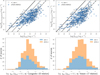Fig. A.1.

Comparison of the jet power (P_jet) and jet production efficiency (η_jet) between the two methods by Cavagnolo et al. (2010) and Ineson et al. (2017). (Top) Correlation between the jet power (P_jet) and bolometric AGN luminosity (L_AGN,bol). The black solid, dashed, and dot-dashed line shows the case with the jet production efficiency η_jet = 1, η_jet = 0.1, and η_jet = 0.01, respectively, by assuming the radiation efficiency of η_rad = 0.1 (Soltan 1982). The other symbols are the same as in Figure 1. (Bottom) Distribution of η_jet assuming the radiative efficiency of 0.1. The left panel shows the result using the relation by Cavagnolo et al. (2010), and the right panel shows the result using the relation by Ineson et al. (2017).

For η_jet, the median value for sources with L_AGN,bol < 10⁴⁵ erg s⁻¹ is ⟨log η_jet⟩= − 1.0 ± 0.6 (Cavagnolo et al. 2010) and ⟨log η_jet⟩= − 1.2 ± 0.6 (Ineson et al. 2017). For high-luminosity sources with L_AGN,bol > 10⁴⁵ erg s⁻¹, the median value is respectively ⟨log η_jet⟩= − 2.0 ± 0.7 (Cavagnolo et al. 2010) and ⟨log η_jet⟩= − 2.0 ± 0.7 (Ineson et al. 2017).

The bottom panels of Figure A.1 show the distribution of η_jet derived from the two relations. As shown in the figures, η_jet ≃ 1 sources still exist even when using the relation of Ineson et al. (2017), while the number of η_jet ≃ 1 sources decreases from 14 sources to 10. Thus, we conclude that the different P_jet − L_radio relation does not affect our main results and discussions.

All Figures

Fig. 1.

Logarithmic value of radio loudness (log ℛ_obs = log(F_int/F_i-band)) vs. the observed i_AB band magnitude of our sample (see Sect. 2.3 for the definition). The original WERGS sample (3579 sources) from Yamashita et al. (2018) are shown as gray circles. The finally selected 393 eFEDS-WERGS sources are shown as blue circles. The eFEDS-WERGS sources with spec-z are highlighted with gray open squares. The statistical errors of both values are vanishingly small, and are therefore not shown.

In the text

Fig. 2.

Luminosities of eFEDS-WERGS sample as a function of redshift. The points are the same as in Fig. 1. Top: rest-frame radio luminosity log L_1.4 GHz (W Hz⁻¹) as a function of redshift, where L_1.4 GHz is obtained from VLA/FIRST (Helfand et al. 2015), and the k-correction was made by Yamashita et al. (2018) based on redshift. The green stars and orange circle and red star points are data obtained from the FIRST-SDSS (Best & Heckman 2012) and VLA-COSMOS catalog, respectively. Middle: 0.5−2 keV AGN luminosity ( $L_{0.5 - 2 keV}^{(abs, corr)}$ ${L_{0.5{-}2\,{\rm keV}}^{\rm (abs,corr)}}$ ) as a function of redshift. The red-filled circle with error bar represents the break luminosity at 0.5−2 keV obtained from Hasinger et al. (2005). Bottom: 12 μm luminosity L_12 μm (erg s⁻¹) as a function of redshift. The k-correction is made by assuming the AGN SED of Mullaney et al. (2011). The red filled circle with error bar represents the break luminosity estimated from the IR AGN studies (Delvecchio et al. 2014).

In the text

Fig. 3.

Obscuration properties of the eFEDS-WERGS sample. Top left: histogram of log(N_H/cm⁻²). The sources are divided into two subgroups with spec-z (cyan) and phot-z (orange). Top right: log N_H as a function of redshift. The gray error bar shows a typical logarithmic error of log N_H. Bottom left: log N_H as a function of 0.5−2 KeV X-ray luminosity ( $L_{0.5 - 2 keV}^{(abs, corr)}$ ${L_{0.5{-}2\,{\rm keV}}^{\rm (abs,corr)}}$ ). The orange shaded area represents the region of obscured AGN with log(N_H/cm⁻²) > 22. The symbols are same as in Fig. 1, and the gray error bar shows a typical logarithmic error of log N_H and log $L_{0.5 - 2 keV}^{(abs, corr)}$ ${L_{0.5{-}2\,{\rm keV}}^{\rm (abs,corr)}}$ . Bottom right: relation between the flux density ratio of 12 μm to optical i_AB band and the log (N_H/cm⁻²). The dashed black line represents the slope of the fitting. The red shaded area represents the region of extremely red quasars which fulfill f_ν(12 μm)/f_ν, i-band > 10^1.84 (Hamann et al. 2017). The orange shaded area represents the obscured AGN region. The other symbols are the same as in Fig. 1.

In the text

Fig. 4.

X-ray and optical spectral properties of three X-ray obscured radio galaxies at z > 3 obtained by this study. Top: X-ray spectra of the three obscured radio galaxies at z > 3. All three sources are spec-z confirmed sources. The left panel is ERO_ID = 3682, z = 3.10, log(N_H/cm⁻²) = 22.1. The middle panel is ERO_ID = 3933, z = 3.09, log(N_H/cm⁻²) = 22.1. The right panel is ERO_ID = 7772, z = 3.11, log(N_H/cm⁻²) = 22.0. The best-fit model and its 99% confidence interval are displayed as blue shaded regions. For each source, the lower panel displays the ratio to the best-fit model. Bottom: optical spectra of the three obscured radio galaxies at z > 3. The spectra for ERO_ID = 3682 and 7772 are taken from the SDSS survey (Abdurro’uf et al. 2022) and the spectrum for ERO_ID = 3933 is taken from the WiggleZ survey, which uses AAT/AAOmega spectrograph (Drinkwater et al. 2018).

In the text

Fig. 5.

Correlation between the luminosities at absorption corrected 2−10 keV ( $L_{2 - 10 keV}^{(abs, corr)}$ ${L_{2{-}10\,{\rm keV}}^{\rm (abs,corr)}}$ ) and 6 μm (L_6 μm). The symbols are the same as in Fig. 1. The red dashed and green dot-dashed line represents the slope in the study of optically selected radio-quiet quasars at 1.5 < z < 5 by Stern (2015) and Chen et al. (2017), respectively.

In the text

Fig. 6.

Relation between the jet and accretion disk properties. Left: correlation between the luminosities at 1.4 GHz (L_1.4 GHz [erg s⁻¹]) and absorption corrected 2−10 keV ( $L_{2 - 10 keV}^{(abs, corr)}$ ${L_{2{-}10\,{\rm keV}}^{\rm (abs,corr)}}$ ). The two black dashed lines in the lower and higher $L_{2 - 10 keV}^{(abs, corr)}$ ${L_{2{-}10\,{\rm keV}}^{\rm (abs,corr)}}$ with the boundary of $L_{2 - 10 keV}^{(abs, corr)} = 10^{44}$ ${L_{2{-}10\,{\rm keV}}^{\rm (abs,corr)}} = 10^{44}$ erg s⁻¹ represent the fitting lines of Eqs. (3) and (4), respectively. Right: correlation between the jet power (P_jet) and bolometric AGN luminosity (L_AGN,bol). The black solid, dashed, and dot-dashed line shows the case with the jet production efficiency η_jet = 1, η_jet = 0.1, and η_jet = 0.01, respectively, by assuming the radiation efficiency of η_rad = 0.1 (Soltan 1982). The other symbols are the same as in Fig. 1.

In the text

	Fig. 7. Distribution of P_jet/erg s⁻¹ (left) and η_jet assuming the radiative efficiency of 0.1 (right). The sample is divided into subgroups of spec-z sources (cyan) and photo-z sources (orange).
In the text

Fig. 8.

Relation between sBHAR (=L_AGN,bol/M_⋆ erg s $^{- 1} M_{⊙}^{- 1}$ $^{-1}\,M_{\odot}^{-1}$ ) and M_⋆. The gray cross represents the typical error bar of the two values. The orange shaded area represents the region of super-Eddington λ_Edd > 1. The three straight lines (from top to bottom) are the expected Eddington ratio of λ_Edd = 1 (Eddington limit; black solid line), λ_Edd = 0.01 (black dashed line), and λ_Edd = 10⁻⁴ (black dot-dashed line) using Eq. (7). The pale pink stars in the background represent the sources from the original WERGS sample with IR detections (KI+21; Ichikawa et al. 2021). The other symbols are the same as in Fig. 1.

In the text

	Fig. 9. Black hole mass estimated from the fundamental plane as a function of redshift. The orange shaded area represents the over-massive SMBH region above the maximum mass limit of known SMBHs (e.g., Kormendy & Ho 2013).
In the text

Fig. 10.

Relations between the values obtained from the BH fundamental plane and those obtained in this study. Top left: relation between two different BH mass estimations. M_BH,FP is obtained from the fundamental plane of Gültekin et al. (2019) and by using the obtained X-ray and radio luminosities in this study. M_BH, ⋆ is the BH mass estimated from the scaling relation of Kormendy & Ho (2013) and by using the obtained stellar mass. The gray cross represents the typical error bar of the two parameters. The gray dashed line represents the 1:1 line with the scatter area of the typical error bar. Top right: relation between the L_{5 GHz, FIRST} and L_{5 GHz, FP}, which is estimated from the fundamental plane relation of Gültekin et al. (2019) with the values of M_BH, ⋆ and $L_{2 - 10 keV}^{(abs, corr)}$ ${L_{2{-}10\,{\rm keV}}^{\rm (abs,corr)}}$ . The gray cross represents the typical error bar of the two parameters. The gray dashed line represents the 1:1 line, with the scatter area of the typical error bar. Bottom left: black hole mass ratio of M_BH,FP/M_BH, ⋆ as a function of ℛ_obs. Bottom right: radio-luminosity ratio of L_{5 GHz, FIRST}/L_{5 GHz, FP} as a function of ℛ_obs. The orange shaded area represents the possible Doppler boost area by assuming typical radio-loud AGN. The red shaded area represents the possible range of the ℛ_obs for blazars by assuming a blazar sequence at 0 < z < 5. The gray cross represents the typical error bar of the two values in each panel.

In the text

Fig. 11.

Radio-luminosity ratio of L_{5 GHz, FIRST}/L_{5 GHz, FP} as a function of sBHAR. The yellow shaded area represents the corresponding Eddington limit accretion (λ_Edd = 1) region assuming the local scaling relation of M_BH − M_⋆ (Kormendy & Ho 2013) for the range of 9 < log(M_⋆/M_⊙) < 12 where our sources reside, as shown in Fig. 8. The gray cross represents the typical error bar of the two values.

In the text

Fig. A.1.

Comparison of the jet power (P_jet) and jet production efficiency (η_jet) between the two methods by Cavagnolo et al. (2010) and Ineson et al. (2017). (Top) Correlation between the jet power (P_jet) and bolometric AGN luminosity (L_AGN,bol). The black solid, dashed, and dot-dashed line shows the case with the jet production efficiency η_jet = 1, η_jet = 0.1, and η_jet = 0.01, respectively, by assuming the radiation efficiency of η_rad = 0.1 (Soltan 1982). The other symbols are the same as in Figure 1. (Bottom) Distribution of η_jet assuming the radiative efficiency of 0.1. The left panel shows the result using the relation by Cavagnolo et al. (2010), and the right panel shows the result using the relation by Ineson et al. (2017).

In the text

Current usage metrics show cumulative count of Article Views (full-text article views including HTML views, PDF and ePub downloads, according to the available data) and Abstracts Views on Vision4Press platform.

Data correspond to usage on the plateform after 2015. The current usage metrics is available 48-96 hours after online publication and is updated daily on week days.

Initial download of the metrics may take a while.

[1] Abdurro’uf, Accetta, K., Aerts, C., et al. 2022, ApJS, 259, 35 [CrossRef] [Google Scholar]

[2] Abramowicz, M. A., Czerny, B., Lasota, J. P., & Szuszkiewicz, E. 1988, ApJ, 332, 646 [Google Scholar]

[3] Ahumada, R., Prieto, C. A., Almeida, A., et al. 2020, ApJS, 249, 3 [Google Scholar]

[4] Aihara, H., Arimoto, N., Armstrong, R., et al. 2018a, PASJ, 70, S4 [NASA ADS] [Google Scholar]

[5] Aihara, H., Armstrong, R., Bickerton, S., et al. 2018b, PASJ, 70, S8 [NASA ADS] [Google Scholar]

[6] Aird, J., Coil, A. L., Moustakas, J., et al. 2012, ApJ, 746, 90 [CrossRef] [Google Scholar]

[7] Aird, J., Coil, A. L., & Georgakakis, A. 2019, MNRAS, 484, 4360 [NASA ADS] [CrossRef] [Google Scholar]

[8] Alonso-Herrero, A., Ramos Almeida, C., Mason, R., et al. 2011, ApJ, 736, 82 [NASA ADS] [CrossRef] [Google Scholar]

[9] An, T., & Baan, W. A. 2012, ApJ, 760, 77 [Google Scholar]

[10] Antonucci, R. 1993, ARA&A, 31, 473 [Google Scholar]

[11] Arnouts, S., Cristiani, S., Moscardini, L., et al. 1999, MNRAS, 310, 540 [Google Scholar]

[12] Asmus, D., Gandhi, P., Hönig, S. F., Smette, A., & Duschl, W. J. 2015, MNRAS, 454, 766 [NASA ADS] [CrossRef] [Google Scholar]

[13] Balbus, S. A., & Hawley, J. F. 1991, ApJ, 376, 214 [Google Scholar]

[14] Baldi, R. D., Capetti, A., & Giovannini, G. 2015, A&A, 576, A38 [NASA ADS] [CrossRef] [EDP Sciences] [Google Scholar]

[15] Baldi, R. D., Capetti, A., & Massaro, F. 2018, A&A, 609, A1 [NASA ADS] [CrossRef] [EDP Sciences] [Google Scholar]

[16] Baldry, I. K., Liske, J., Brown, M. J. I., et al. 2018, MNRAS, 474, 3875 [Google Scholar]

[17] Baldwin, J. E. 1982, in Extragalactic Radio Sources, eds. D. S. Heeschen, & C. M. Wade, 97, 21 [NASA ADS] [Google Scholar]

[18] Bañados, E., Venemans, B. P., Mazzucchelli, C., et al. 2018, Nature, 553, 473 [Google Scholar]

[19] Baron, D., & Ménard, B. 2019, MNRAS, 487, 3404 [CrossRef] [Google Scholar]

[20] Becker, R. H., White, R. L., & Helfand, D. J. 1995, ApJ, 450, 559 [Google Scholar]

[21] Best, P. N., & Heckman, T. M. 2012, MNRAS, 421, 1569 [NASA ADS] [CrossRef] [Google Scholar]

[22] Best, P. N., Kauffmann, G., Heckman, T. M., & Ivezić, Ž. 2005, MNRAS, 362, 9 [Google Scholar]

[23] Birrer, S., & Amara, A. 2018, Phys. Dark Univ., 22, 189 [Google Scholar]

[24] Birrer, S., Amara, A., & Refregier, A. 2015, ApJ, 813, 102 [Google Scholar]

[25] Bîrzan, L., McNamara, B. R., Nulsen, P. E. J., Carilli, C. L., & Wise, M. W. 2008, ApJ, 686, 859 [Google Scholar]

[26] Blandford, R., Meier, D., & Readhead, A. 2019, ARA&A, 57, 467 [NASA ADS] [CrossRef] [Google Scholar]

[27] Blundell, K. M., Rawlings, S., & Willott, C. J. 1999, AJ, 117, 677 [Google Scholar]

[28] Boquien, M., Burgarella, D., Roehlly, Y., et al. 2019, A&A, 622, A103 [NASA ADS] [CrossRef] [EDP Sciences] [Google Scholar]

[29] Bosch, J., Armstrong, R., Bickerton, S., et al. 2018, PASJ, 70, S5 [Google Scholar]

[30] Brandt, W. N., & Alexander, D. M. 2015, A&ARv, 23, 1 [Google Scholar]

[31] Brinkmann, W., Laurent-Muehleisen, S. A., Voges, W., et al. 2000, A&A, 356, 445 [NASA ADS] [Google Scholar]

[32] Brunner, H., Liu, T., Lamer, G., et al. 2022, A&A, 661, A1 [NASA ADS] [CrossRef] [EDP Sciences] [Google Scholar]

[33] Brusa, M., Urrutia, T., Toba, Y., et al. 2022, A&A, 661, A9 [NASA ADS] [CrossRef] [EDP Sciences] [Google Scholar]

[34] Bruzual, G., & Charlot, S. 2003, MNRAS, 344, 1000 [NASA ADS] [CrossRef] [Google Scholar]

[35] Buchner, J., Georgakakis, A., Nandra, K., et al. 2015, ApJ, 802, 89 [Google Scholar]

[36] Calzetti, D., Armus, L., Bohlin, R. C., et al. 2000, ApJ, 533, 682 [NASA ADS] [CrossRef] [Google Scholar]

[37] Capetti, A., Massaro, F., & Baldi, R. D. 2017, A&A, 598, A49 [NASA ADS] [CrossRef] [EDP Sciences] [Google Scholar]

[38] Cavagnolo, K. W., McNamara, B. R., Nulsen, P. E. J., et al. 2010, ApJ, 720, 1066 [Google Scholar]

[39] Chabrier, G. 2003, PASP, 115, 763 [Google Scholar]

[40] Chen, C. T. J., Brandt, W. N., Reines, A. E., et al. 2017, ApJ, 837, 48 [NASA ADS] [CrossRef] [Google Scholar]

[41] Chen, X., Ichikawa, K., Noda, H., et al. 2020, ApJ, 905, L2 [Google Scholar]

[42] Chiaberge, M., & Marconi, A. 2011, MNRAS, 416, 917 [Google Scholar]

[43] Ciotti, L., Ostriker, J. P., & Proga, D. 2009, ApJ, 699, 89 [NASA ADS] [CrossRef] [Google Scholar]

[44] Condon, J. J. 1992, ARA&A, 30, 575 [Google Scholar]

[45] Corbel, S., Nowak, M. A., Fender, R. P., Tzioumis, A. K., & Markoff, S. 2003, A&A, 400, 1007 [NASA ADS] [CrossRef] [EDP Sciences] [Google Scholar]

[46] Coriat, M., Fender, R. P., & Dubus, G. 2012, MNRAS, 424, 1991 [NASA ADS] [CrossRef] [Google Scholar]

[47] Croom, S. M., Richards, G. T., Shanks, T., et al. 2009, MNRAS, 392, 19 [CrossRef] [Google Scholar]

[48] Daly, R. A., Sprinkle, T. B., O’Dea, C. P., Kharb, P., & Baum, S. A. 2012, MNRAS, 423, 2498 [NASA ADS] [CrossRef] [Google Scholar]

[49] de Gasperin, F., Intema, H. T., & Frail, D. A. 2018, MNRAS, 474, 5008 [Google Scholar]

[50] Delvecchio, I., Gruppioni, C., Pozzi, F., et al. 2014, MNRAS, 439, 2736 [NASA ADS] [CrossRef] [Google Scholar]

[51] Delvecchio, I., Smolčić, V., Zamorani, G., et al. 2018, MNRAS, 481, 4971 [Google Scholar]

[52] Dey, A., Schlegel, D. J., Lang, D., et al. 2019, AJ, 157, 168 [Google Scholar]

[53] Donato, D., Ghisellini, G., Tagliaferri, G., & Fossati, G. 2001, A&A, 375, 739 [NASA ADS] [CrossRef] [EDP Sciences] [Google Scholar]

[54] Dong, A.-J., & Wu, Q. 2015, MNRAS, 453, 3447 [Google Scholar]

[55] Drinkwater, M. J., Byrne, Z. J., Blake, C., et al. 2018, MNRAS, 474, 4151 [Google Scholar]

[56] Dunlop, J. S., & Peacock, J. A. 1990, MNRAS, 247, 19 [NASA ADS] [Google Scholar]

[57] Fabian, A. C. 2012, ARA&A, 50, 455 [Google Scholar]

[58] Falcke, H., Körding, E., & Markoff, S. 2004, A&A, 414, 895 [NASA ADS] [CrossRef] [EDP Sciences] [Google Scholar]

[59] Finlez, C., Treister, E., Bauer, F., et al. 2022, ApJ, 936, 88 [NASA ADS] [CrossRef] [Google Scholar]

[60] Fossati, G., Maraschi, L., Celotti, A., Comastri, A., & Ghisellini, G. 1998, MNRAS, 299, 433 [Google Scholar]

[61] Furusawa, H., Koike, M., Takata, T., et al. 2018, PASJ, 70, S3 [Google Scholar]

[62] Gaia Collaboration (Brown, A. G. A., et al.) 2018, A&A, 616, A1 [NASA ADS] [CrossRef] [EDP Sciences] [Google Scholar]

[63] Gallo, E., Fender, R. P., & Pooley, G. G. 2003, MNRAS, 344, 60 [Google Scholar]

[64] Gandhi, P., Horst, H., Smette, A., et al. 2009, A&A, 502, 457 [NASA ADS] [CrossRef] [EDP Sciences] [Google Scholar]

[65] Ghisellini, G., Tavecchio, F., Maraschi, L., Celotti, A., & Sbarrato, T. 2014, Nature, 515, 376 [NASA ADS] [CrossRef] [Google Scholar]

[66] Ghisellini, G., Righi, C., Costamante, L., & Tavecchio, F. 2017, MNRAS, 469, 255 [NASA ADS] [CrossRef] [Google Scholar]

[67] Gültekin, K., King, A. L., Cackett, E. M., et al. 2019, ApJ, 871, 80 [Google Scholar]

[68] Haardt, F., & Maraschi, L. 1991, ApJ, 380, L51 [Google Scholar]

[69] Hamann, F., Zakamska, N. L., Ross, N., et al. 2017, MNRAS, 464, 3431 [Google Scholar]

[70] Hannikainen, D. C., Hunstead, R. W., Campbell-Wilson, D., & Sood, R. K. 1998, A&A, 337, 460 [NASA ADS] [Google Scholar]

[71] Hardcastle, M. J. 2018, MNRAS, 475, 2768 [Google Scholar]

[72] Hardcastle, M. J., Williams, W. L., Best, P. N., et al. 2019, A&A, 622, A12 [NASA ADS] [CrossRef] [EDP Sciences] [Google Scholar]

[73] Harwood, J. J., Hardcastle, M. J., Croston, J. H., & Goodger, J. L. 2013, MNRAS, 435, 3353 [NASA ADS] [CrossRef] [Google Scholar]

[74] Hasinger, G., Miyaji, T., & Schmidt, M. 2005, A&A, 441, 417 [NASA ADS] [CrossRef] [EDP Sciences] [Google Scholar]

[75] Hawley, J. F., & Balbus, S. A. 2002, ApJ, 573, 738 [NASA ADS] [CrossRef] [Google Scholar]

[76] Heckman, T. M., & Best, P. N. 2014, ARA&A, 52, 589 [Google Scholar]

[77] Heinz, S., & Merloni, A. 2004, MNRAS, 355, L1 [NASA ADS] [CrossRef] [Google Scholar]

[78] Heinz, S., & Sunyaev, R. A. 2003, MNRAS, 343, L59 [Google Scholar]

[79] Helfand, D. J., White, R. L., & Becker, R. H. 2015, ApJ, 801, 26 [NASA ADS] [CrossRef] [Google Scholar]

[80] HI4PI Collaboration (Ben Bekhti, N., et al.) 2016, A&A, 594, A116 [NASA ADS] [CrossRef] [EDP Sciences] [Google Scholar]

[81] Hickox, R. C., Jones, C., Forman, W. R., et al. 2009, ApJ, 696, 891 [Google Scholar]

[82] Ho, L. C. 2008, ARA&A, 46, 475 [Google Scholar]

[83] Holt, J., Tadhunter, C. N., & Morganti, R. 2008, MNRAS, 387, 639 [NASA ADS] [CrossRef] [Google Scholar]

[84] Huang, S., Leauthaud, A., Murata, R., et al. 2018, PASJ, 70, S6 [CrossRef] [Google Scholar]

[85] Hwang, H.-C., Zakamska, N. L., Alexandroff, R. M., et al. 2018, MNRAS, 477, 830 [CrossRef] [Google Scholar]

[86] Ichikawa, K., Ueda, Y., Terashima, Y., et al. 2012, ApJ, 754, 45 [Google Scholar]

[87] Ichikawa, K., Packham, C., Ramos Almeida, C., et al. 2015, ApJ, 803, 57 [NASA ADS] [CrossRef] [Google Scholar]

[88] Ichikawa, K., Ueda, J., Shidatsu, M., Kawamuro, T., & Matsuoka, K. 2016, PASJ, 68, 9 [NASA ADS] [CrossRef] [Google Scholar]

[89] Ichikawa, K., Ricci, C., Ueda, Y., et al. 2017, ApJ, 835, 74 [NASA ADS] [CrossRef] [Google Scholar]

[90] Ichikawa, K., Ricci, C., Ueda, Y., et al. 2019a, ApJ, 870, 31 [NASA ADS] [CrossRef] [Google Scholar]

[91] Ichikawa, K., Kawamuro, T., Shidatsu, M., et al. 2019b, ApJ, 883, L13 [NASA ADS] [CrossRef] [Google Scholar]

[92] Ichikawa, K., Yamashita, T., Toba, Y., et al. 2021, ApJ, 921, 51 [NASA ADS] [CrossRef] [Google Scholar]

[93] Ichimaru, S. 1977, ApJ, 214, 840 [NASA ADS] [CrossRef] [Google Scholar]

[94] Igumenshchev, I. V., & Abramowicz, M. A. 1999, MNRAS, 303, 309 [NASA ADS] [CrossRef] [Google Scholar]

[95] Ilbert, O., Arnouts, S., McCracken, H. J., et al. 2006, A&A, 457, 841 [NASA ADS] [CrossRef] [EDP Sciences] [Google Scholar]

[96] Inayoshi, K., Haiman, Z., & Ostriker, J. P. 2016, MNRAS, 459, 3738 [NASA ADS] [CrossRef] [Google Scholar]

[97] Inayoshi, K., Ichikawa, K., & Haiman, Z. 2018, ApJ, 863, L36 [NASA ADS] [CrossRef] [Google Scholar]

[98] Inayoshi, K., Ichikawa, K., Ostriker, J. P., & Kuiper, R. 2019, MNRAS, 486, 5377 [NASA ADS] [CrossRef] [Google Scholar]

[99] Ineson, J., Croston, J. H., Hardcastle, M. J., & Mingo, B. 2017, MNRAS, 467, 1586 [NASA ADS] [Google Scholar]

[100] Inoue, Y., & Totani, T. 2009, ApJ, 702, 523 [NASA ADS] [CrossRef] [Google Scholar]

[101] Inoue, Y., Doi, A., Tanaka, Y. T., Sikora, M., & Madejski, G. M. 2017, ApJ, 840, 46 [NASA ADS] [CrossRef] [Google Scholar]

[102] Ishino, T., Matsuoka, Y., Koyama, S., et al. 2020, PASJ, 72, 83 [NASA ADS] [CrossRef] [Google Scholar]

[103] Isobe, T., Feigelson, E. D., Akritas, M. G., & Babu, G. J. 1990, ApJ, 364, 104 [Google Scholar]

[104] Ivezić, Ž., Menou, K., Knapp, G. R., et al. 2002, AJ, 124, 2364 [CrossRef] [Google Scholar]

[105] Jimenez-Gallardo, A., Massaro, F., Capetti, A., et al. 2019, A&A, 627, A108 [NASA ADS] [CrossRef] [EDP Sciences] [Google Scholar]

[106] Jones, D. H., Read, M. A., Saunders, W., et al. 2009, MNRAS, 399, 683 [Google Scholar]

[107] Jun, H. D., Im, M., Lee, H. M., et al. 2015, ApJ, 806, 109 [CrossRef] [Google Scholar]

[108] Jurlin, N., Brienza, M., Morganti, R., et al. 2021, A&A, 653, A110 [NASA ADS] [CrossRef] [EDP Sciences] [Google Scholar]

[109] Kaiser, C. R., Dennett-Thorpe, J., & Alexander, P. 1997, MNRAS, 292, 723 [Google Scholar]

[110] Kawanomoto, S., Uraguchi, F., Komiyama, Y., et al. 2018, PASJ, 70, 66 [Google Scholar]

[111] Keel, W. C., Maksym, W. P., Bennert, V. N., et al. 2015, AJ, 149, 155 [NASA ADS] [CrossRef] [Google Scholar]

[112] Keel, W. C., Lintott, C. J., Maksym, W. P., et al. 2017, ApJ, 835, 256 [NASA ADS] [CrossRef] [Google Scholar]

[113] Kellermann, K. I., Sramek, R., Schmidt, M., Shaffer, D. B., & Green, R. 1989, AJ, 98, 1195 [Google Scholar]

[114] Kimball, A. E., Kellermann, K. I., Condon, J. J., Ivezić, Ž., & Perley, R. A. 2011, ApJ, 739, L29 [NASA ADS] [CrossRef] [Google Scholar]

[115] Komissarov, S. S., & Gubanov, A. G. 1994, A&A, 285, 27 [NASA ADS] [Google Scholar]

[116] Komiyama, Y., Obuchi, Y., Nakaya, H., et al. 2018, PASJ, 70, S2 [Google Scholar]

[117] Kormendy, J., & Ho, L. C. 2013, ARA&A, 51, 511 [Google Scholar]

[118] Li, Z.-Y., Wu, X.-B., & Wang, R. 2008, ApJ, 688, 826 [NASA ADS] [CrossRef] [Google Scholar]

[119] Li, J., Silverman, J. D., Ding, X., et al. 2021, ApJ, 918, 22 [NASA ADS] [CrossRef] [Google Scholar]

[120] Li, J., Silverman, J. D., Merloni, A., et al. 2023, MNRAS, submitted [arXiv:2302.12438] [Google Scholar]

[121] Liska, M., Tchekhovskoy, A., Ingram, A., & van der Klis, M. 2019, MNRAS, 487, 550 [CrossRef] [Google Scholar]

[122] Liu, T., Buchner, J., Nandra, K., et al. 2022, A&A, 661, A5 [NASA ADS] [CrossRef] [EDP Sciences] [Google Scholar]

[123] Lopez-Rodriguez, E., Packham, C., Tadhunter, C., et al. 2014, ApJ, 793, 81 [NASA ADS] [CrossRef] [Google Scholar]

[124] Lopez-Rodriguez, E., Alonso-Herrero, A., Diaz-Santos, T., et al. 2018, MNRAS, 478, 2350 [NASA ADS] [CrossRef] [Google Scholar]

[125] Lubow, S. H., Papaloizou, J. C. B., & Pringle, J. E. 1994, MNRAS, 267, 235 [NASA ADS] [Google Scholar]

[126] Luo, A. L., Zhao, Y.-H., Zhao, G., et al. 2015, RAA, 15, 1095 [NASA ADS] [Google Scholar]

[127] Maraschi, L., & Rovetti, F. 1994, ApJ, 436, 79 [NASA ADS] [CrossRef] [Google Scholar]

[128] Marconi, A., Risaliti, G., Gilli, R., et al. 2004, MNRAS, 351, 169 [Google Scholar]

[129] Mason, R. E., Lopez-Rodriguez, E., Packham, C., et al. 2012, AJ, 144, 11 [NASA ADS] [CrossRef] [Google Scholar]

[130] Massaro, E., Maselli, A., Leto, C., et al. 2015, Ap&SS, 357, 75 [Google Scholar]

[131] Mateos, S., Carrera, F. J., Alonso-Herrero, A., et al. 2015, MNRAS, 449, 1422 [Google Scholar]

[132] Matsuta, K., Gandhi, P., Dotani, T., et al. 2012, ApJ, 753, 104 [NASA ADS] [CrossRef] [Google Scholar]

[133] Mauch, T., & Sadler, E. M. 2007, MNRAS, 375, 931 [Google Scholar]

[134] McConnell, N. J., Ma, C.-P., Gebhardt, K., et al. 2011, Nature, 480, 215 [NASA ADS] [CrossRef] [Google Scholar]

[135] McKinney, J. C., Tchekhovskoy, A., Sadowski, A., & Narayan, R. 2014, MNRAS, 441, 3177 [NASA ADS] [CrossRef] [Google Scholar]

[136] McNamara, B. R., & Nulsen, P. E. J. 2007, ARA&A, 45, 117 [NASA ADS] [CrossRef] [Google Scholar]

[137] Merloni, A., Heinz, S., & di Matteo, T. 2003, MNRAS, 345, 1057 [Google Scholar]

[138] Merloni, A., Predehl, P., Becker, W., et al. 2012, ArXiv e-prints [arXiv:1209.3114] [Google Scholar]

[139] Merloni, A., Bongiorno, A., Brusa, M., et al. 2014, MNRAS, 437, 3550 [Google Scholar]

[140] Miyazaki, S., Komiyama, Y., Kawanomoto, S., et al. 2018, PASJ, 70, S1 [NASA ADS] [Google Scholar]

[141] Morgan, C. W., Kochanek, C. S., Morgan, N. D., & Falco, E. E. 2010, ApJ, 712, 1129 [Google Scholar]

[142] Morganti, R., Tadhunter, C. N., & Oosterloo, T. A. 2005, A&A, 444, L9 [NASA ADS] [CrossRef] [EDP Sciences] [Google Scholar]

[143] Morganti, R., Jurlin, N., Oosterloo, T., et al. 2021, Galaxies, 9, 88 [NASA ADS] [CrossRef] [Google Scholar]

[144] Mortlock, D. J., Warren, S. J., Venemans, B. P., et al. 2011, Nature, 474, 616 [Google Scholar]

[145] Mullaney, J. R., Alexander, D. M., Goulding, A. D., & Hickox, R. C. 2011, MNRAS, 414, 1082 [Google Scholar]

[146] Mullaney, J. R., Daddi, E., Béthermin, M., et al. 2012, ApJ, 753, L30 [Google Scholar]

[147] Narayan, R., & Yi, I. 1994, ApJ, 428, L13 [Google Scholar]

[148] Narayan, R., & Yi, I. 1995, ApJ, 444, 231 [Google Scholar]

[149] Narayan, R., Igumenshchev, I. V., & Abramowicz, M. A. 2000, ApJ, 539, 798 [NASA ADS] [CrossRef] [Google Scholar]

[150] Nemmen, R. S., & Tchekhovskoy, A. 2015, MNRAS, 449, 316 [NASA ADS] [CrossRef] [Google Scholar]

[151] Nesvadba, N. P. H., De Breuck, C., Lehnert, M. D., Best, P. N., & Collet, C. 2017, A&AS, 599, A123 [NASA ADS] [CrossRef] [EDP Sciences] [Google Scholar]

[152] Nishizawa, A. J., Hsieh, B. C., Tanaka, M., & Takata, T. 2020, ArXiv e-prints [arXiv:2003.01511] [Google Scholar]

[153] Ohsuga, K., Mori, M., Nakamoto, T., & Mineshige, S. 2005, ApJ, 628, 368 [NASA ADS] [CrossRef] [Google Scholar]

[154] Ohsuga, K., Mineshige, S., Mori, M., & Kato, Y. 2009, PASJ, 61, L7 [NASA ADS] [Google Scholar]

[155] Onoue, M., Kashikawa, N., Matsuoka, Y., et al. 2019, ApJ, 880, 77 [Google Scholar]

[156] Orr, M. J. L., & Browne, I. W. A. 1982, MNRAS, 200, 1067 [CrossRef] [Google Scholar]

[157] Padovani, P. 2016, A&ARv, 24, 13 [Google Scholar]

[158] Pflugradt, J., Ichikawa, K., Akiyama, M., et al. 2022, ApJ, 938, 75 [NASA ADS] [CrossRef] [Google Scholar]

[159] Predehl, P., Andritschke, R., Arefiev, V., et al. 2021, A&A, 647, A1 [EDP Sciences] [Google Scholar]

[160] Privon, G. C., Baum, S. A., O’Dea, C. P., et al. 2012, ApJ, 747, 46 [NASA ADS] [CrossRef] [Google Scholar]

[161] Rafferty, D. A., McNamara, B. R., Nulsen, P. E. J., & Wise, M. W. 2006, ApJ, 652, 216 [NASA ADS] [CrossRef] [Google Scholar]

[162] Rakshit, S., Stalin, C. S., & Kotilainen, J. 2020, ApJS, 249, 17 [Google Scholar]

[163] Ramos Almeida, C., Levenson, N. A., Rodríguez Espinosa, J. M., et al. 2009, ApJ, 702, 1127 [NASA ADS] [CrossRef] [Google Scholar]

[164] Ricci, C., Ueda, Y., Koss, M. J., et al. 2015, ApJ, 815, L13 [Google Scholar]

[165] Ricci, C., Trakhtenbrot, B., Koss, M. J., et al. 2017, ApJS, 233, 17 [Google Scholar]

[166] Ross, N. P., Hamann, F., Zakamska, N. L., et al. 2015, MNRAS, 453, 3932 [Google Scholar]

[167] Ross, N. P., Ford, K. E. S., Graham, M., et al. 2018, MNRAS, 480, 4468 [Google Scholar]

[168] Ruiz, A., Corral, A., Mountrichas, G., & Georgantopoulos, I. 2018, A&A, 618, A52 [NASA ADS] [CrossRef] [EDP Sciences] [Google Scholar]

[169] Ryan, B. R., Ressler, S. M., Dolence, J. C., et al. 2017, ApJ, 844, L24 [NASA ADS] [CrossRef] [Google Scholar]

[170] Saade, M. L., Brightman, M., Stern, D., Malkan, M. A., & García, J. A. 2022, ApJ, 936, 162 [NASA ADS] [CrossRef] [Google Scholar]

[171] Sadler, E. M., Jackson, C. A., Cannon, R. D., et al. 2002, MNRAS, 329, 227 [Google Scholar]

[172] Salvato, M., Hasinger, G., Ilbert, O., et al. 2009, ApJ, 690, 1250 [CrossRef] [Google Scholar]

[173] Salvato, M., Ilbert, O., Hasinger, G., et al. 2011, ApJ, 742, 61 [Google Scholar]

[174] Salvato, M., Buchner, J., Budavári, T., et al. 2018, MNRAS, 473, 4937 [Google Scholar]

[175] Salvato, M., Wolf, J., Dwelly, T., et al. 2022, A&A, 661, A3 [NASA ADS] [CrossRef] [EDP Sciences] [Google Scholar]

[176] Sartori, L. F., Schawinski, K., Koss, M. J., et al. 2018, MNRAS, 474, 2444 [NASA ADS] [CrossRef] [Google Scholar]

[177] Schawinski, K., Evans, D. A., Virani, S., et al. 2010, ApJ, 724, L30 [NASA ADS] [CrossRef] [Google Scholar]

[178] Schinnerer, E., Smolčić, V., Carilli, C. L., et al. 2007, ApJS, 172, 46 [Google Scholar]

[179] Schirmer, M., Malhotra, S., Levenson, N. A., et al. 2016, MNRAS, 463, 1554 [NASA ADS] [CrossRef] [Google Scholar]

[180] Schlafly, E. F., Meisner, A. M., & Green, G. M. 2019, ApJS, 240, 30 [Google Scholar]

[181] Schmitt, J. H. M. M. 1985, ApJ, 293, 178 [NASA ADS] [CrossRef] [Google Scholar]

[182] Shabala, S. S., & Godfrey, L. E. H. 2013, ApJ, 769, 129 [NASA ADS] [CrossRef] [Google Scholar]

[183] Shabala, S. S., Jurlin, N., Morganti, R., et al. 2020, MNRAS, 496, 1706 [NASA ADS] [CrossRef] [Google Scholar]

[184] Shen, Y., Richards, G. T., Strauss, M. A., et al. 2011, ApJS, 194, 45 [Google Scholar]

[185] Sikora, M., Stawarz, Ł., & Lasota, J.-P. 2007, ApJ, 658, 815 [NASA ADS] [CrossRef] [Google Scholar]

[186] Smolčić, V., Novak, M., Bondi, M., et al. 2017a, A&A, 602, A1 [Google Scholar]

[187] Smolčić, V., Delvecchio, I., Zamorani, G., et al. 2017b, A&A, 602, A2 [NASA ADS] [CrossRef] [EDP Sciences] [Google Scholar]

[188] Soltan, A. 1982, MNRAS, 200, 115 [Google Scholar]

[189] Stern, D. 2015, ApJ, 807, 129 [Google Scholar]

[190] Stone, J. M., & Pringle, J. E. 2001, MNRAS, 322, 461 [CrossRef] [Google Scholar]

[191] Stone, J. M., Pringle, J. E., & Begelman, M. C. 1999, MNRAS, 310, 1002 [Google Scholar]

[192] Sunyaev, R., Arefiev, V., Babyshkin, V., et al. 2021, A&A, 656, A132 [NASA ADS] [CrossRef] [EDP Sciences] [Google Scholar]

[193] Tadhunter, C. 2016, A&ARv, 24, 10 [Google Scholar]

[194] Takeo, E., Inayoshi, K., & Mineshige, S. 2020, MNRAS, 497, 302 [NASA ADS] [CrossRef] [Google Scholar]

[195] Tanaka, M., Coupon, J., Hsieh, B.-C., et al. 2018, PASJ, 70, S9 [Google Scholar]

[196] Tchekhovskoy, A., Narayan, R., & McKinney, J. C. 2011, MNRAS, 418, L79 [NASA ADS] [CrossRef] [Google Scholar]

[197] Toba, Y., Yamashita, T., Nagao, T., et al. 2019, ApJS, 243, 15 [Google Scholar]

[198] Toba, Y., Liu, T., Urrutia, T., et al. 2022, A&A, 661, A15 [NASA ADS] [CrossRef] [EDP Sciences] [Google Scholar]

[199] Trakhtenbrot, B. 2014, ApJ, 789, L9 [NASA ADS] [CrossRef] [Google Scholar]

[200] Truemper, J. 1993, Science, 260, 1769 [Google Scholar]

[201] Uchiyama, H., Yamashita, T., Toshikawa, J., et al. 2022a, ApJ, 926, 76 [NASA ADS] [CrossRef] [Google Scholar]

[202] Uchiyama, H., Yamashita, T., Nagao, T., et al. 2022b, PASJ, 74, L27 [NASA ADS] [CrossRef] [Google Scholar]

[203] Ueda, J., Iono, D., Yun, M. S., et al. 2014, ApJS, 214, 1 [Google Scholar]

[204] Urry, C. M., & Padovani, P. 1995, PASP, 107, 803 [NASA ADS] [CrossRef] [Google Scholar]

[205] van Velzen, S., & Falcke, H. 2013, A&A, 557, L7 [NASA ADS] [CrossRef] [EDP Sciences] [Google Scholar]

[206] Villar-Martín, M., Cabrera-Lavers, A., Humphrey, A., et al. 2018, MNRAS, 474, 2302 [Google Scholar]

[207] Wang, R., Wu, X.-B., & Kong, M.-Z. 2006, ApJ, 645, 890 [NASA ADS] [CrossRef] [Google Scholar]

[208] White, R. L., Becker, R. H., Helfand, D. J., & Gregg, M. D. 1997, ApJ, 475, 479 [Google Scholar]

[209] Willott, C. J., Rawlings, S., Blundell, K. M., & Lacy, M. 1999, MNRAS, 309, 1017 [Google Scholar]

[210] Willott, C. J., Rawlings, S., Blundell, K. M., Lacy, M., & Eales, S. A. 2001, MNRAS, 322, 536 [NASA ADS] [CrossRef] [Google Scholar]

[211] Wright, E. L., Eisenhardt, P. R. M., Mainzer, A. K., et al. 2010, AJ, 140, 1868 [Google Scholar]

[212] Wu, X.-B., Wang, F., Fan, X., et al. 2015, Nature, 518, 512 [Google Scholar]

[213] Wylezalek, D., Zakamska, N. L., Greene, J. E., et al. 2018, MNRAS, 474, 1499 [NASA ADS] [CrossRef] [Google Scholar]

[214] Xie, F.-G., & Yuan, F. 2012, MNRAS, 427, 1580 [NASA ADS] [CrossRef] [Google Scholar]

[215] Yamashita, T., Nagao, T., Akiyama, M., et al. 2018, ApJ, 866, 140 [NASA ADS] [CrossRef] [Google Scholar]

[216] Yamashita, T., Nagao, T., Ikeda, H., et al. 2020, AJ, 160, 60 [NASA ADS] [CrossRef] [Google Scholar]