| Issue |
A&A
Volume 686, June 2024
|
|
|---|---|---|
| Article Number | A155 | |
| Number of page(s) | 29 | |
| Section | Interstellar and circumstellar matter | |
| DOI | https://doi.org/10.1051/0004-6361/202348983 | |
| Published online | 07 June 2024 | |
Cloud properties across spatial scales in simulations of the interstellar medium
1
AIM, CEA, CNRS, Université Paris-Saclay, Université Paris Diderot, Sorbonne Paris Cité,
91191
Gif-sur-Yvette,
France
e-mail: This email address is being protected from spambots. You need JavaScript enabled to view it.
2
Universität Heidelberg, Zentrum für Astronomie, Institut für Theoretische Astrophysik,
Albert-Ueberle-Str. 2,
69120
Heidelberg,
Germany
e-mail: This email address is being protected from spambots. You need JavaScript enabled to view it.
; This email address is being protected from spambots. You need JavaScript enabled to view it.
3
INAF – Istituto di Astrofisica e Planetologia Spaziali,
via Fosso del Cavaliere 100,
00133
Roma,
Italy
4
Institute of Physics, Laboratory for Galaxy Evolution and Spectral Modelling, EPFL, Observatoire de Sauverny,
Chemin Pegasi 51,
1290
Versoix,
Switzerland
5
Universität Heidelberg, Interdisziplinäres Zentrum für Wissenschaftliches Rechnen,
Im Neuenheimer Feld 205,
69120
Heidelberg,
Germany
6
Laboratoire de Physique de l’École Normale Supérieure, ENS, Université PSL, CNRS, Sorbonne Université, Université de Paris,
75005
Paris,
France
Received:
17
December
2023
Accepted:
1
March
2024
Abstract
Context. Molecular clouds (MCs) are structures of dense gas in the interstellar medium (ISM) that extend from ten to a few hundred parsecs and form the main gas reservoir available for star formation. Hydrodynamical simulations of a varying complexity are a promising way to investigate MCs evolution and their properties. However, each simulation typically has a limited range in resolution and different cloud extraction algorithms are used, which complicates the comparison between simulations.
Aims. In this work, we aim to extract clouds from different simulations covering a wide range of spatial scales. We compare their properties, such as size, shape, mass, internal velocity dispersion, and virial state.
Methods. We applied the HOP cloud detection algorithm on (M)HD numerical simulations of stratified ISM boxes and isolated galactic disk simulations that were produced using FLASH, RAMSES, and AREPO.
Results. We find that the extracted clouds are complex in shape, ranging from round objects to complex filamentary networks in all setups. Despite the wide range of scales, resolution, and sub-grid physics, we observe surprisingly robust trends in the investigated metrics. The mass spectrum matches in the overlap between simulations without rescaling and with a high-mass power-law index of −1 for logarithmic bins of mass, in accordance with theoretical predictions. The internal velocity dispersion scales with the size of the cloud as σ ∝ R0.75 for large clouds (R ≳ 3 pc). For small clouds we find larger σ compared to the power-law scaling, as seen in observations, which is due to supernova-driven turbulence. Almost all clouds are gravitationally unbound with the virial parameter scaling as αvir ∝ M−04, which is slightly flatter compared to observed scaling but in agreement given the large scatter. We note that the cloud distribution towards the low-mass end is only complete if the more dilute gas is also refined, rather than only the collapsing regions.
Key words: methods: numerical / ISM: clouds
© The Authors 2024
 Open Access article, published by EDP Sciences, under the terms of the Creative Commons Attribution License (https://creativecommons.org/licenses/by/4.0), which permits unrestricted use, distribution, and reproduction in any medium, provided the original work is properly cited.
This article is published in open access under the Subscribe to Open model. This email address is being protected from spambots. You need JavaScript enabled to view it. to support open access publication.
1 Introduction
Historically, (molecular) clouds have been considered important building blocks in the interstellar medium (ISM). The warm and diffuse gas condenses to form cloud-like structures with masses of ~104−106 M⊙, typical sizes of ~10 − 100 pc, mean densities of ![Mathematical equation: $\[n_{\mathrm{H}_2}\]$](/articles/aa/full_html/2024/06/aa48983-23/aa48983-23-eq1.png) ~ 100 cm−3, and temperatures of T ~ 10 K (e.g. Solomon et al. 1987; Scoville et al. 1987; Dame et al. 1987, 2001, or Klessen & Glover 2016 for a review). Most of the mass in these conditions is in the form of molecular hydrogen, and hence the term molecular clouds (MCs). However, most of the dynamical properties and the connection to hydrodynamical evolution does not require the gas being molecular. One particularly important aspect connected to clouds is that they harbour the coldest (~ 10 K) regions of the ISM including the collapsing cores that eventually form stars.
~ 100 cm−3, and temperatures of T ~ 10 K (e.g. Solomon et al. 1987; Scoville et al. 1987; Dame et al. 1987, 2001, or Klessen & Glover 2016 for a review). Most of the mass in these conditions is in the form of molecular hydrogen, and hence the term molecular clouds (MCs). However, most of the dynamical properties and the connection to hydrodynamical evolution does not require the gas being molecular. One particularly important aspect connected to clouds is that they harbour the coldest (~ 10 K) regions of the ISM including the collapsing cores that eventually form stars.
For a long time, clouds were considered to be stable and long-lived structures that are gravitationally bound and supported against collapse by magnetic fields, for example (e.g. Mouschovias & Spitzer 1976; Shu et al. 1987; Mouschovias & Ciolek 1999). This paradigm has changed. In particular, the idea that clouds are magnetically supported has given way to a picture in which they are formed by a combination of gravity and turbulence (e.g. Ballesteros-Paredes et al. 1999; Ballesteros-Paredes & Mac Low 2002; Mac Low & Klessen 2004; Krumholz & McKee 2005; Ballesteros-Paredes 2006; Hennebelle & Chabrier 2008; Ballesteros-Paredes et al. 2011; Vázquez-Semadeni et al. 2017, 2019), with the magnetic field playing an important but not dominant role (e.g. Crutcher 2012; Girichidis 2021; Whitworth et al. 2023). Turbulence creates over-densities and large-scale coherent structures, whose shapes are similar to the complex shapes of molecular clouds (e.g. Schneider et al. 2011; Ebagezio et al. 2023). As a result, the gas in the ISM is constantly reshaped by turbulence without permanent structures on a crossing time tcross = L/υ, where L is the cloud size and υ the local velocity dispersion on a scale L. In the solar neighbourhood, representative values for L and υ are 30 pc and 3 km s−1, respectively, yielding tcross ~ 10 Myr, a small fraction of the orbital period of the Galaxy. Clouds can form in regions of converging flows and are dispersed by shear and/or feedback from stars (e.g. Chevance et al. 2023, for a recent review). Therefore, molecular clouds should not be regarded as well-defined discrete entities with clearly identifiable boundaries.
Larson (1981) was the first to establish power-law scaling relations between molecular cloud properties. He observed that cloud mass and size followed the relation M ∝ R1.90 while the velocity dispersion scaled as σν ∝ R0.38. Both of these relations showed significant scatter. In the Milky Way and neighbouring galaxies, MCs seem to adhere to the Larson relations, where the non-thermal line-width increases with cloud size following an approximate power law of index one half (Larson 1981; Solomon et al. 1987; Bolatto et al. 2008; Fukui et al. 2008; Heyer et al. 2009; Roman-Duval et al. 2010; Wong et al. 2011). This relation extends within clouds (Heyer & Brunt 2004) and may be attributed to the power-law scaling expected for compressible turbulence (McKee & Ostriker 2007). Larson (1981) also argued that MCs exhibited similar levels of kinetic and gravitational energy and hence were approximately in virial equilibrium (see also Blitz 1993). This can be quantified through the use of the virial parameter (Bertoldi & McKee 1992)
![Mathematical equation: $\[\alpha_{\text {vir }} \equiv \frac{5 \sigma_v^2 R}{G M},\]$](/articles/aa/full_html/2024/06/aa48983-23/aa48983-23-eq2.png) (1)
(1)
in which σν is the one-dimensional velocity dispersion, G is the gravitational constant, and R and M are the size and mass of the cloud, respectively. Virial equilibrium corresponds to αvir = 1. Although early studies of massive clouds found that αvir ~ 1, more recent surveys that are sensitive to a much broader range of cloud masses find a more complex picture (Heyer et al. 2001; Oka et al. 2001; Gratier et al. 2012; Donovan Meyer et al. 2013; Rice et al. 2016; Miville-Deschênes et al. 2017; Colombo et al. 2019; Rosolowsky et al. 2021). These surveys show that low-mass clouds are unbound with virial ratios ≫ 1 and only massive clouds with masses of order 106 M⊙ or more are marginally bound. However, there are large uncertainties involved in determining the mass of MCs from observations (Szűcs et al. 2016), and so the characteristic mass at which MCs become gravitationally bound has been difficult to determine accurately. Clouds with virial parameters exceeding unity mostly follow a relation with αvir ∝ M−1/2 (Chevance et al. 2023).
The formation of MCs and the dynamical evolution of the gas within them has been addressed in hydrodynamical simulations with a range of different complexities. Early studies either focussed on simulating isolated clouds (Vazquez-Semadeni et al. 1995; Stone et al. 1998; Klessen & Burkert 2000; Ostriker et al. 2001; Bate et al. 2003; Padoan et al. 2007) or covered large fractions of the interstellar medium without resolving the interior of clouds (de Avillez 2000; de Avillez & Breitschwerdt 2005; Joung & Mac Low 2006; Kim & Ostriker 2007; Hill et al. 2012; Gent et al. 2013; Walch et al. 2012). However, increasing computational power now allows us to cover both the large-scale environment, including the hot and dilute gas from which clouds condense as well as the coldest collapsing phases. Seifried et al. (2017) showed the importance of embedding the clouds into the turbulent large-scale (~100 pc) environment, in order to accurately follow the turbulent cascade and the formation of cold gas. They adopted a zoom-in approach in which they followed the evolution of individual clouds selected from a large-scale simulation of the ISM with successively improving resolution. This approach allowed them to reach resolutions as small as 0.1 pc, but limited them to modelling only a few clouds, thereby preventing them from drawing robust statistical conclusions. A companion study at a lower resolution of 0.25 pc by Girichidis (2021) complements these efforts. Both models only consider environmental conditions similar to the solar neighbourhood. Similar simulations of stratified boxes but with different turbulent driving recipes and total gas masses have been performed by other groups (e.g. Joung et al. 2009; Simpson et al. 2016; Martizzi et al. 2016; Kim & Ostriker 2017; Brucy et al. 2020, 2023; Colman et al. 2022). These simulations cover slightly larger scales and employ different cooling recipes. In addition, it has now become possible to carry out simulations of entire disk galaxies with a resolution sufficient to resolve individual clouds, allowing one to study the roles of global galactic rotation and differential shear and to cover a large range of local surface densities (e.g. Tress et al. 2020, 2021; Jeffreson et al. 2020). All of these models have their own strengths and weaknesses in terms of physical processes included, environmental properties of molecular clouds and maximum resolution. Therefore, an important question to ask prior to comparing the results of these simulations to observations is whether the predictions of different simulations for the properties of the MCs distribution agree with one other, that is whether these predictions are robust to changes in the numerical approach. Because the definition of a cloud is not trivial, it is important to use the same cloud extraction method with identical parameters for cloud identification, so that we can be sure that any differences we find are due to differences in the simulations and not in the cloud identification algorithm. A thorough comparison between numerical models in overlapping ranges of the cloud masses is crucial for verifying that the full range of cloud masses and sizes can be compared to observations without numerically induced breaks in the scaling relations. Furthermore, a comparison between simulations can be considerably more detailed than a comparison with observations, as we have the full 3D distribution of all relevant physical variables available for our simulated clouds, which is not the case for real, observed MCs.
In this paper, we investigate the molecular cloud properties in a variety of numerical simulations with different resolutions and different numerical recipes for cooling, star formation and stellar feedback. Our goal is to verify the existence of smooth transitions between the simulations and quantify the clouds in terms of global properties that can be transferred to the observational domain. Our study is structured as follows: in Sec. 2 we discuss the algorithm used to extract the clouds and the numerical simulations on which the algorithm was applied. Then, in Sec. 3, we compare the cloud population’s masses, sizes and shapes. In Sec. 4 we focus on the internal properties of the clouds, looking at the thermal state, the turbulence and the gravitational stability. We discuss the importance of resolution and of the specifics of the cloud extraction process in Sec. 5 and conclude in Sec. 6.
Set of simulations.
2 Numerical methods, simulation data
2.1 Structure finding algorithm
Our structure finding algorithm is built around the HOP clump finder (Eisenstein & Hut 1998). While originally it was developed for finding groups of particles in N-body simulations, the algorithm and its original implementation are quite general and can be used in many more applications. One advantage HOP has is that it simply requires a list of particles as input. While this may seem sub-optimal for analysing regular grid-based hydrodynamics simulations, it allows for a direct comparison between the results of particle-based codes, unstructured meshes as well as regular grid-based (AMR) codes. To achieve this, we transform the AMR grid into a list of cells.
Overall, there are three steps towards obtaining a structure catalogue, which are described in depth in Appendix A. First, we use HOP to identify peak patches around local density maxima. Then, we use the regrouping tool from HOP to merge peaks based on a number of specified criteria. For clouds, we adopt a density threshold of 30 cm−3. Everything below this threshold is not considered to be part of a cloud. Then we require a cloud to have a peak density of at least 60 cm−3, which corresponds to a minimum peak-to-background ratio of 2. When the saddle density between two structures is larger than 300 cm−3, that is to say ten times the density threshold, we consider them as being substructures within the same cloud and therefore merge them. Lastly, we require a structure to be made up of at least 100 cells. After this merging step, we know for each cell or particle the structure to which it belongs, or whether it does not belong to any structure. Based on that, we then finally calculate the properties of all identified structures as detailed in Appendix A.
2.2 Numerical simulations of the ISM
We apply the HOP algorithm to several (M)HD simulations of the ISM. We combine simulations with a wide range of simulation techniques, resolution, box size and physics included. An overview is given in Table 1. A face-on projection of one snapshot of each simulation type is featured in Fig. 1, where we over-plot the positions of the extracted clouds colour-coded by their derived velocity dispersion for illustration.
2.2.1 SILCC: Stratified boxes with FLASH
We include high-resolution magnetised simulations from the SILCC collaboration (Walch et al. 2015; Girichidis et al. 2016), which are described in detail in Girichidis et al. (2018) and Girichidis (2021). The setup consists of a stratified box with a volume of 0.5 × 0.5 × 0.5 kpc3. The gas is initially at rest and in hydrostatic equilibrium with a total gas mass surface density of 10 M⊙ pc−2. The two different magnetic field models considered here have central magnetic field strengths at z = 0 of Bx,0 = 3 μG and Bx,0 = 6 μG and are oriented along the x direction. The field strength scales vertically with the gas density as Bx(z) = Bx,0 [ρ(z)/ρ(z = 0)]1/2. The initial setup is magnetically supercritical, that is the field cannot support the gas against collapse.
The MHD equations are solved using the HLLR5 solver (Bouchut et al. 2007, 2010; Waagan 2009; Waagan et al. 2011), which is implemented in FLASH in Version 4 (Fryxell et al. 2000; Dubey et al. 2008). Heating of the gas includes spatially clustered supernovae (SNe), as well as cosmic ray (Goldsmith & Langer 1978) and X-ray heating (Wolfire et al. 1995). The CR ionisation and heating rates are ζcr = 3 × 10⁻¹⁷ s−1 and ΓCR = 3.2 × 10⁻¹¹ ζCR n erg s−1 cm−3, respectively. Photoelectric heating follows Bakes & Tielens (1994), Bergin et al. (2004) and Wolfire et al. (2003). We assume a spatially constant interstellar radiation field (ISRF) with a strength of 1.7 in the units of the Habing field G0 (Habing 1968; Draine 1978) that is then locally attenuated in dense, shielded gas using the TreeCol algorithm (Clark et al. 2012; Wünsch et al. 2018). We fix the dust-to-gas mass ratio to 0.01, and adopt dust opacities from Mathis et al. (1983) for wavelengths shorter than 1 μm and Ossenkopf & Henning (1994) for longer wavelengths.
Heating and radiative cooling processes are computed using a chemical network that tracks the non-equilibrium concentrations of ionised hydrogen (H+), atomic hydrogen (H), molecular hydrogen (H2), as well as singly ionised carbon (C+) and carbon monoxide (CO). The hydrogen chemistry is based on the models by Hollenbach & McKee (1989); Glover & Mac Low (2007a,b) and Micic et al. (2012). The reactions connected to CO follow the model developed by Nelson & Langer (1997). Radiative cooling incorporates contributions from the fine structure lines of C+, O, and Si+. Furthermore, we consider rotational and vibrational lines of H2 and CO, as well as Lyman-α cooling. The energy transfer from the gas to the dust follows Glover et al. (2010) and Glover & Clark (2012a). Above 104 K, we assume collisional ionisation equilibrium (CIE) for helium and all heavy elements, and adopt the corresponding CIE cooling rates from Gnat & Ferland (2012). Hydrogen is not assumed to be in collisional ionisation equilibrium, and its contribution to the cooling process is calculated self-consistently at all temperatures, accounting for any deviations from chemical equilibrium.
Gravitational forces include self-gravity as well as an external potential based on an isothermal sheet (Spitzer 1942) with a surface density of 30 M⊙ pc−2, representing the stellar mass distribution. The vertical scale height of this sheet is set to 100 pc. The Poisson equation is solved using the tree-based method as described in Wünsch et al. (2018).
Star formation and the related supernova feedback are included at a fixed rate. We derive a star formation rate based on the Kennicutt-Schmidt relation (Kennicutt 1998) and convert it to a SN rate using the Chabrier (2003) IMF. This yields 15 SNe per Myr for the volume simulated here. Each explosion injects 1051 erg of thermal energy. For the positioning of the SNe we distinguish between a type Ia (20%) and a type II component (80%). The type Ia SNe are individual explosions placed at random (uniformly chosen) positions for x and y. The z position is randomly sampled from a Gaussian distribution with a vertical scale height of 300 pc (Bahcall & Soneira 1980; Heiles 1987), where we ensure that SNe that are placed outside the box are re-drawn to be placed inside the box. The type II SNe are further split into isolated SNe (40% of the type II) and clustered counterparts (60%) (Heiles 1987; Kennicutt et al. 1989; McKee & Williams 1997; Clarke & Oey 2002). For the positioning of the individual type II SNe and the clusters we also chose random positions for x and y. The vertical distribution is drawn from a Gaussian with a smaller scale height of 90 pc. All SNe within a cluster explode at the same cluster position. The positions of the SNe are computed beforehand and stored in a table to ensure an identical feedback configuration for the different magnetic field strengths and resolutions.
We consider three different resolutions for the simulations. In all cases, the base resolution is 1283, corresponding to a maximum cubic cell with a side length of 3.9 pc. On top we add two additional levels of refinement for simulations SILCC-1pc-3 μG and SILCC-1pc-6 μG, which reach a minimum cell size of 0.98 pc. For simulations SILCC-0.5pc-3μG and SILCC-0.25pc-3μG we restart simulation SILCC-1pc-3μG at a time of 20 Myr and add one and two additional levels of refinement, which yields minimum cell sizes of 0.49 and 0.24 pc, respectively. The simulations with a resolution of 1 pc run for a total time of 60 Myr; the higher resolution ones were evolved for a shorter time of a few Myr (Girichidis 2021).
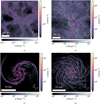 |
Fig. 1 Column density map for a single snapshot from each of the four listed groups of simulations. The panels show SILCC-0.5pc-3μG (a), LS-weak-driving (b), M51 (c), Ramses-F20 (d). Details of these simulations can be found in Table 1. The coloured symbols indicate the locations of the clouds identified by the HOP algorithm, with the colour corresponding to the internal velocity dispersion. |
2.2.2 LS: Stratified boxes with RAMSES
For our comparison, we also use RAMSES (Teyssier 2002) simulations of a stratified piece of a galactic disk. The simulations are fully described in Colman et al. (2022) and references therein. The computational domain is cubic with a box size of 1 kpc. The base grid with a resolution of 3.9 pc is further refined using a mass-based criterion up to a minimum cell size of 0.24 pc in the densest regions. Compared to the SILCC simulations, the computational domain is larger, but the different refinement strategy can results in fewer AMR grids (see discussion in Sec. 5.1).
The initial density profile is Gaussian n(z) = n0 exp[−0.5 (z/z0)2] with a mid-plane particle density n0 = 1.5 cm−3 and a thickness z0 = 150 pc, corresponding to a column density of ∑ = 19.1 M⊙ pc−2. An initial level of turbulence is introduced by adding a turbulent velocity field with a root mean square dispersion of 5 km s−1 and a Kolmogorov power spectrum E(k) ∝ k−5/3 with random phase. The initial temperature is 5333 K, which is a typical value for the warm neutral medium phase in the ISM. We also include a magnetic field oriented along the x-axis with Bx(z) = B0 exp[−0.5 (z/z0)2] initially, where B0 = 7.62 μG is the mid-plane field strength. The magnetic field is solved using the ideal MHD approximation, as implemented by Fromang et al. (2006). Aside from self-gravity, we also apply an external gravitational disk potential as prescribed by Kuijken & Gilmore (1989) and Joung & Mac Low (2006), which accounts for the profile of (old) stars and dark matter.
We use an ISM cooling model based on Audit & Hennebelle (2005) that includes the most important processes responsible for regulating the thermal balance of the atomic ISM. At low temperatures, cooling is provided by the fine structure transitions of C+ and O, while at high temperatures this is supplemented by contributions from grain surface recombination of atomic hydrogen and from Lyman-α cooling. Heating is provided primarily by the photoelectric effect, calculated assuming a constant uniform UV background with a strength equal to the solar neighbourhood value. In contrast to the SILCC and AREPO simulations, we do not account for local attenuation of this radiation field within dense clouds. We also account for cosmic ray heating, using the rate given in Goldsmith (2001). The ionisation of hydrogen is treated by the RT module from Rosdahl et al. (2013). We use sink particles to track star formation and stellar feedback self-consistently. Sinks represent newly formed star clusters (Bleuler & Teyssier 2014), which accrete gas which is within a 4 cell accretion radius and above the sink formation threshold of 104 cm−3. Each time a sink has accreted enough mass, it forms a massive star particle with a mass between 8 and 120 M⊙ randomly drawn from the Salpeter IMF (Salpeter 1955). This massive star emits ionising radiation and explodes as a supernova at the end of its lifetime (Rosdahl et al. 2013; Geen et al. 2016; Colling et al. 2018). The radiation is treated using a moment-based method (Rosdahl et al. 2013). In addition to the turbulence generated by stellar feedback, we also include external driving on scales between 1 box length and 1/3 of the box length with solenoidal fraction 0.75. Several forcing strengths were explored: weak, medium and strong driving, as well as no driving, which result in mass weighted velocity dispersions of σ3D ≈ 9, 12, 20 and 8.5 km s−1, respectively. The simulations were evolved for 60 Myr.
2.2.3 M51: Full galaxy with AREPO
Stratified box set-ups allow one to simulate the ISM at high resolution but miss important aspects linked to large scales: self-consistent large-scale driving, galactic dynamical effects such as rotation or the influence of spiral density waves, and large-scale instabilities such as the Toomre instability (Toomre 1964) or the wiggle instability (Sormani et al. 2017). As this may influence the properties of the clouds that form in the ISM, we included two full galaxy simulations in our study. The first one was carried out using AREPO, a moving-mesh hydrodynamic code (Springel 2010), and was fully presented in Tress et al. (2020). The clouds from this simulation were already extracted and analysed in Tress et al. (2021), but with a different cloud extraction algorithm. The modelled galaxy is interacting with a smaller companion and its properties are chosen to be similar to the M51 ‘Whirlpool’ galaxy. The characteristics of the different components (dark matter halo, stellar bulge, stellar disk and gaseous disk) are summarised in Table B.1. Gravitational interactions between all those components were self-consistently accounted for.
Resolution in AREPO is defined by the target mass, which is the typical mass of a cell. This is analogous to the particle mass in an smoothed particle hydrodynamics (SPH) computation. For the M51 simulation, the target mass is 300 M⊙, with additional refinement in the denser part of the ISM such that the Jeans length is resolved by at least four cells up to a density of 10−21 g cm−3. As a result of this refinement scheme, most of the cells above the HOP density threshold have a radius of 1 pc or less, with the smallest cells having a radius of only 0.4 pc. For comparison with the minimum Δx in the AMR simulations, we quote in Table 1 the typical diameter of a cell at the sink creation density threshold, which is ~1.4 pc. The effective resolution of this simulation in dense regions is thus slightly worse than the low resolution SILCC runs.
Unlike the previous sets of simulations, the magnetic field is not modelled. The thermal and chemical evolution of the gas are solved simultaneously, using the NL97 chemical network described in Glover & Clark (2012b) and the atomic and molecular cooling function described in Clark et al. (2019). Star formation is modelled using sink particles that are created within gravitationally bound regions of radius 2.5 pc when the gas density exceeds a threshold of 10−21 g cm−3, if the region satisfies several additional criteria: it must be a local minimum of the gravitational potential, and both the velocity and the acceleration must be converging. Once formed, sink particles can accrete gas from within an accretion radius of 2.5 pc, with the accretion limited to gas with a density exceeding the sink creation density. Two feedback processes are modelled: type II and type Ia SNe. The type II SNe are attached to the sinks, via a process similar to the one described in Sect. 2.2.2. Type Ia SNe are exploded at the position of a randomly selected old star with a rate of one explosion every 250 yr. These are the stellar particles of the disk and bulge components of the N-body model of the galaxy. Supernovae were modelled by injecting energy in a region containing 40 resolution elements surrounding the injection region. Momentum or thermal energy is injected based on whether the Sedov-Taylor phase is resolved.
2.2.4 Ramses-F20: Full galaxy with RAMSES
To complete the study, we also ran the algorithm on a isolated disk simulation performed with RAMSES that was initially presented in Brucy (2022, Chapter 11). The model is an isolated disk with a radius of 15 kpc, within a box with a side length of 120 kpc. Initial conditions are generated with the code DICE, which allow one to specify the different components of a galaxy. DICE generates particles representing dark matter, stars and gas. The two first are directly used in RAMSES while the gas distribution was mapped from the particles onto the AMR grid. The parameters for the generation of the initial conditions are summed up in Table B.1.
Using the adaptive mesh refinement capabilities of RAMSES, the maximal cell size is 1 kpc outside the disk and 7 pc within the disk. The minimal cell size is 0.92 pc within the disk. Dark matter and initial stars are modelled via particles that only undergo gravity. The gas follows the law of hydrodynamics (without magnetic field) and gravity. The simulation is run over a period of 300 Myr.
The simulation also includes a sub-grid model for star formation and stellar feedback, here limited to SN explosions and photo-ionisation-triggered heating. These models are those developed and described in Kretschmer & Teyssier (2020). The star formation rate is computed for each cell from its properties. First the Mach number ℳ within the cell is computed thanks to a model of the evolution of the sub-grid turbulent velocity. This is then used to estimate the sub-grid density PDF, assuming that it is a log-normal (Vazquez-Semadeni 1994; Federrath & Klessen 2012), as well as the virial parameter of the cell. The expected star formation rate within the cell is then computed using the multi-free-fall analytical model for the star formation rate adapted from Krumholz et al. (2005) by Hennebelle & Chabrier (2011) and popularised by Federrath & Klessen (2012). At each time-step the number of new star particles created is randomly drawn from a Poisson distribution, calibrated so that the mean star formation rate over time is equal to the one given by the analytical model. The SN injection scheme depend whether the cooling radius the SN is resolved by a least one grid cell. If yes, the energy from the explosion is directly injected in the form of thermal energy. Otherwise, the terminal momentum of the SN is also injected. Photo-ionisation is modelled by maintaining the cell where the star sits at a temperature of 104 K until the last SN explodes. The cooling method is the same as the one used in the RAMSES stratified box simulation presented in Sect. 2.2.2.
2.3 Examples of extracted clouds
Figure 2 displays some examples of extracted objects in the various simulations. The images show the projected column density in a region around the clouds, so we can also see their environment. The white contours show the projected cloud boundaries. The mass and velocity dispersion are listed at the top of the image. A coloured symbol is assigned to each example cloud, which will be used to identify them in further figures.
The column density projections illustrate the wide variety in sizes and shapes we find. The clouds range from simple roundish shapes to very complex structures, which cannot be captured with simple measures such as the sphericity or the triaxiality. This is particularly clear when comparing the projected images for the LS clouds in Fig. 2b with a 3D rendering of the same clouds in Fig. 3, where we also show the ellipsoid approximation to the cloud from which its size is estimated (see Sec. 3 and Appendix A.3). In most cases, the cloud’s shape is far from ellipsoid (see also Ebagezio et al. 2023). However the corresponding sizes give a reasonable approximation to the extent of the objects. We also note that projection effects are significant. Especially large clouds can appear quite different when viewing them from different angles. Furthermore, there are often multiple clouds along the same line of sight. Consequently, the projections along the line of sight are limited to the cloud under consideration and its direct environment rather than being the integration throughout the entire simulation box.
In the stratified box simulations, large clouds are filamentary in nature and their internal structure is resolved. Small clouds typically do not have a resolved substructure and appear more regular in shape, which is true for all simulations. In the galaxy simulations, some of the largest clouds have disk-like shapes as illustrated in the left panel of Figs. 2c and 2d. These are unrealistic and result from a lack of resolution.
2.4 Notes on comparing with cloud catalogues from observations
Many catalogues of ISM structures have been compiled from observations using various techniques. A complete and robust comparison of simulation results to these catalogues requires the creation of synthetic observations, which could then be processed by the same pipeline as the observations to extract the clouds in the exact same way. This is clearly beyond the scope of this work. Nevertheless, it is useful to compare the trends we find in the simulations, which will be discussed in the following sections, to the ones observed in the Milky Way and nearby galaxies.
The classic molecular cloud catalogues are obtained from CO observations. The main CO isotopologue, 12CO, is detectable at relatively low densities (Snow & McCall 2006), potentially as low as our cloud extraction density threshold of 30 cm−3, provided there is molecular gas at these densities. Emission lines from the 13CO isotopologue trace somewhat higher densities. The spectral information can be used to try to disentangle overlapping projected clouds. The observed line-width of the transition is assumed to be set mainly by turbulence. While the dimension of the observed clouds is typically derived from the circularised radius of the cloud area in all the catalogues, the mass is derived with different methods that include different assumptions and approximations. A key parameter in the mass and radius estimate is the distance of the cloud. In the Milky Way, this is typically derived using a model for the rotation curve of the Galaxy, a method which is prone to large uncertainties (see e.g. Reid 2022). Thanks to the recent effort to create 3D dust maps (e.g. Chen et al. 2019; Leike et al. 2020), it has become possible to accurately estimate the distances to clouds detected in dust extinction for structures up to a distance of ~400 pc, offering an alternative to CO cloud catalogues. Chen et al. (2020) detected clouds directly in PPP space, but cloud properties were still derived from 2D projections. Very recently, Dharmawardena et al. (2023) and Cahlon et al. (2024) calculated the cloud mass and size from the reconstructed 3D dust density distributions. 3D dust maps do not provide kinematic information and so one cannot recover the velocity dispersion with this data alone. So far, no one has attempted to combine spectral line and 3D dust information to derive cloud velocity dispersion. Extra-galactic surveys of MCs in nearby galaxies do not suffer from the same distance uncertainties, but are typically sensitive to only the most massive MCs in all but the closest Local Group galaxies (Rosolowsky et al. 2021).
All current Milky Way molecular cloud catalogues have specific lower limits in the recoverable masses and radii. In particular, the smallest recoverable radius depends on the spatial resolution of the observations. The smallest observable mass depends on the sensitivity. Both resolution and sensitivity decrease with increasing cloud distance. As a consequence, catalogues such as those of Rice et al. (2016) and Miville-Deschênes et al. (2017) that were derived from the first generations of CO surveys (Dame et al. 2001) with spatial resolution of 8’5 and spectral resolution of 1.3 km s−1 contain on average larger and more massive clouds than more recent compilations of molecular clouds (e.g. Benedettini et al. 2020, 2021; Duarte-Cabral et al. 2021) that are extracted from the new generation of CO surveys with sub-arcminute spatial resolution and spectral resolution well below 1 km s−1. Moreover, in general all the catalogues of the observed molecular clouds are incomplete at the lower masses and radii. The threshold for incompleteness depends on the distance and thus can be variable for catalogues of the entire Milky Way.
It must also be noted that CO, especially 12CO, becomes optically thick in the denser parts of clouds (see e.g. Tielens 2010; Draine 2011). This means that we cannot see beyond a certain maximum surface density, leading us to underestimate of the mass if not properly accounted for, which is hard to do. Dust, on the other hand, is an optically thin tracer and thus does not have this problem. This, and the other remarks made here, must be kept in mind when putting the results described in the next sections into an observational context.
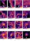 |
Fig. 2 Column density maps of selected clouds extracted from the simulations. The different rows show examples from SILCC-0.5-pc (a), LS-no-driving (b), M51 (c), Ramses-F20 (d). Column density is calculated in a box of three times the maximum extent of the object. Labels are added showing the cloud mass and velocity dispersion. The coloured symbol is used to refer to the cloud in the following figures in the paper. |
 |
Fig. 3 3D visualisations of the clouds from Fig. 2b, extracted from the LS stratified box simulations. The density scale is linear. The ellipsoid approximation (in cyan) and its half-axes (in black) are also shown. |
3 Comparison of cloud mass, size, and shape
We start our comparison of the cloud catalogues by looking at the masses, sizes and shapes of the clouds. The cloud mass is simply the sum of the masses of all of the cells/particles it contains. The size is determined through the diagonalisation of the inertia matrix. Using the resulting eigenvalues, we construct an ellipsoid of uniform density which has the same moments of inertia as the cloud. The size is then taken to be the geometric average of the axis lengths of this ellipsoid. The corresponding equations can be found in Appendix A. Figure 3 illustrates that the ellipsoid approximation traces well the extent of a cloud.
An alternative definition of the size is the cubic root of the total volume of the cloud, which neglects the shape information. In the following, we use both definitions as they provide different insights.
3.1 Mass and size distribution
The mass and size distributions are shown in Fig. 4. To facilitate the comparison, we normalise the histograms according to the surface area covered by the simulation. In other words, the figure shows the number of clouds per unit area (here kpc2). For the stratified box simulations (SILCC and LS), this is straightforward as their computational domain defines the area of the region. For the stratified boxes we combine the catalogues of several individual simulations and/or snapshots into one histogram to keep the plot readable. This is justified because the distributions do not differ significantly. The distribution for SILCC-1pc contains the two SILCC runs with 1 pc resolution and different magnetic field strengths (SILCC-1pc-3 μG and SILCC-1pc-6 μG). The label LS includes all four LS runs with different driving strengths. The number of snapshots used for this compilation is listed in Table 1. The total surface area is then the box area multiplied by the number of snapshots. For the galaxy simulations, the relevant area is less straightforward to define. To get an estimate, we divided the face-on column density image into 1 kpc2 tiles and counted how many of them have an average column density larger than 3 M⊙ pc−2.
3.1.1 Power-law tail
The high-mass end of the mass distribution of clouds is typically described by a power law dN/d log M ∝ Mα, or alternatively dN/dM ∝ Mγ with γ = α − 1, optionally with a truncation. Unless stated differently, listed exponents correspond to α. With the appropriate normalisation, the agreement of the slope of both the mass and size distribution is remarkable. Especially for the mass spectrum which spans six orders of magnitude ranging from giant cloud complexes of 106−107 M⊙ down to tiny cloudlets of barely 10 M⊙. The value of the power-law exponent is close to −1, as indicated by the grey line. The exponent of the size distribution is around −3. For large masses and sizes, we typically see a cut-off in the distributions for the stratified box simulations due to the limited box size and the resulting limited total mass. Since we analyse only a handful of snapshots, values of the histogram below 1 cloud per kpc2 correspond to rare events and are not statistically significant.
The only massive clouds which do not lie on the general mass spectrum are the most massive clouds in the Ramses-F20 simulation, which show an excess compared to the overall trend. We found 286 clouds with a mass above 106 M⊙, indicating that this is not a statistical fluctuation. Furthermore, the cloud mass distribution in this simulation seems to consist of multiple components. Upon closer inspection (cf. Figs. 5 and C.1), we see a secondary peak around 5 × 10⁵ M⊙, indicating an excess of clouds with high masses, in both the Ramses-F20 galaxy and M51. These object are spurious disk-shaped clouds like the examples shown in the left column of Fig. 2c, and thus not physical because of limited resolution. Once formed, they are very difficult to destroy by regular stellar feedback, which is limited as well by the overall worse resolution.
We fitted the mass spectrum slope in the appropriate range for individual simulations (Appendix C). The resulting slopes for the stratified boxed and M51 agree well with one another, ranging from −1.16 to −1.35. Ramses-F20 has a shallower slope of −0.76. This difference is likely related to differences in the numerical feedback recipes used in each simulation. The SN recipe used in Ramses-F20 injects energy or momentum only in one of the cell neighbouring the exploding star, which makes it hard to destroy large structures. Meanwhile, because the injection radius is linked to a minimal number of cells, the recipe used in the AREPO simulation tends to overestimate the feedback effect when the resolution is poor. This difference alone could explain why clouds in Ramses-F20 are typically larger than those in M51.
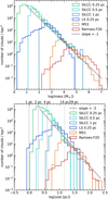 |
Fig. 4 Comparison of the mass (top) and size (bottom) distribution of clouds in the different simulations, normalised according to the relevant surface area of the simulation. To guide the eye, we add a grey line indicating an appropriate power-law slopes of −1 for the mass spectrum in the top panel and −3 for the size distribution in the bottom panel. The dashed lines correspond to multiples of the spacial resolution in the SILCC and LS simulations. The dotted lines show multiples of the resolution for the Ramses galaxy. |
3.1.2 Turn-over and low-mass end
The low-mass end of the spectra are shaped by resolution effects. In all cases, the mass and size distribution is incomplete for values below the peak. The SILCC setups show a relatively sharp cut-off slighty above four times the resolution limit, an effect of our requirement that a cloud has to contain at least 100 cells1. We note that RAMSES simulations (LS and Ramses-F20) have different shapes at the low-mass end, with a much shallower transition between a peak and a low-mass cut-off. We discuss in Sec. 5.1 that this stems from a difference in the grid refinement strategy used in RAMSES and FLASH. For LS, the peak is observed at a value slightly larger than the spatial resolution of the coarse grid (refinement level 8, corresponding to a cell size of 4 pc). For the Ramses-F20 galaxy, it is somewhere between twice and four times the coarse grid resolution. For M51 the cut-off is less straightforward to determine, since both the cell size and the cell mass vary in AREPO simulations. This results in a relatively wide mass and size distribution for the cells. We also typically have overall fewer cells in AREPO runs compared to AMR simulations (FLASH and RAMSES). The combination of these two aspects result in a low cloud mass cut-off that is largely determined by the minimum number of cells for a structure used by HOP, which is 100. At the highest densities reached in the M51 simulation, the typical particle mass is around 10–20 M⊙, and so we see a cut-off in the cloud mass distribution at 100 times this value, namely 1000–2000 M⊙. We note that this cut-off is not as sharp as in the SILCC runs because there are some cells in the M51 simulation with masses below 10 M⊙ and hence HOP identifies a few clouds containing these cells with total masses below 1000 M⊙.
It is worth noting that the ranges of masses and radii measured in observational data are in agreement with the ranges derived from simulations with a minimum cell size comparable to the spatial resolution of the observations. When quoting median values for the property distributions, it thus only makes sense to compare with studies which have comparable resolution.
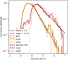 |
Fig. 5 Comparison of the mass distribution of clouds in the inner 7 kpc of a galaxy versus those in the outskirts. While Ramses-F20 overall has a shallower mass spectrum than M51 (and the kpc boxes), there is no difference in the measured slope between the inner and the outer galaxy for either simulation. |
3.1.3 Predictions from theory
Turbulent fragmentation theories predict a mass spectrum with a power law for massive objects on all scales from GMCs to cores. The self-similarity of gravity, which is argued to be the dominant force, results in dN/d log M ∝ Mα with α = −1. Detailed derivations of turbulent fragmentation theories, which take into account several corrections, predict slopes which are slightly shallower (Hennebelle & Chabrier 2008; Hopkins 2012). Also accretion theories predict α = −1 when the accretion rate scales as ![Mathematical equation: $\[\dot{M}\]$](/articles/aa/full_html/2024/06/aa48983-23/aa48983-23-eq3.png) ∝ M2 (Kuznetsova et al. 2018). The global slope we find is indeed close to −1.
∝ M2 (Kuznetsova et al. 2018). The global slope we find is indeed close to −1.
3.1.4 Slope variations in observations
Observationally, the obtained slope varies significantly between studies. Roman-Duval et al. (2010) find α = −1.64 ± 0.25, consistent with the value of −1.5 obtained in older work (Sanders et al. 1985; Solomon et al. 1987; Williams & McKee 1997). Miville-Deschênes et al. (2017) find α = −2.0 ± 0.1 for their full Milky Way catalogue. Rice et al. (2016), who used the same underlying CO data as Miville-Deschênes et al. (2017), report a shallower slope and differences between the outer Galaxy for which α = −1.2 ± 0.1, and the inner Galaxy where α = −0.6 ± 0.1. A similar diversity was obtained by Rosolowsky (2005) who found α = −0.5 ± 0.1 and α = −1.1 ± 0.2 for the inner and outer Milky Way respectively, α = −1.9 ± 0.4 for the M33 galaxy and α = −0.7 ± 0.2 for the Large Magellanic Cloud. A study of the actual M51 galaxy also reports variations with environments: α ≈ −0.3 for the centre and bar, α ≈ −0.8 to −0.6 for the molecular ring and spiral arms and α ≈ −1.5 for the inter-arm and outer galaxy regions (Colombo et al. 2014). Moreover, the mass spectrum is not well-described by a power law in all regions, suggesting different dominant mechanisms for the formation and destruction of clouds in the different parts of the galaxy. In summary, the observed slopes range from as shallow as −0.3 to as steep as −2.0. This variety is in contradiction to the universality of our results which are all fairly close to −1. Figure 5 investigates more closely the mass spectrum in our two galaxy simulations, dividing the cloud population into two groups: clouds in the inner and outer galaxy with the boundary being at 7 kpc from the centre of mass. We find no significant difference in the slope. A small difference in typical cloud mass is obtained for clouds in the very centre of the galaxies, as discussed in Appendix D. A similar trend was already found by Tress et al. (2021), who extracted clouds from their M51 galaxy using a different algorithm than we apply here. Possibly the measured slope depends on the exact method with which clouds have been extracted from observations. The same holds for simulations as will be discussed in Sec. 5.2. We also note also that it can be difficult to estimate the completeness limit, which may also affect the fit of the slope. The situation is even more complex for catalogues for which the cloud distance is not uniform. Since the effective spatial resolution is lower at greater distances, small clouds appear blended into larger objects, which results in a shallower mass spectrum slope. A more rigorous comparison with observations through synthetic observations could provide a more direct conclusion about whether or not the simulation results are in agreement with the observations.
3.2 Mass–size relation
Observations show that cloud properties are not independent from each other (Hennebelle & Falgarone 2012; Heyer & Dame 2015). A tight relation between cloud mass and size is reported by many studies (e.g. Solomon et al. 1987; Roman-Duval et al. 2010; Kauffmann et al. 2013; Miville-Deschênes et al. 2017). In Fig. 6a, we plot the relation between the mass and size of each cloud for the various simulations of our comparison set. We remind the reader that the size of the cloud is defined as the average between the three principal axes, as identified by the structure algorithm. The tight correlation we see with a power-law slope of 3 is expected and is due to the way clouds are extracted. By construction, the mean density of the cloud cannot be below the chosen threshold of 30 cm−3 above which cells are considered by the cloud detection algorithm. Also, it is rather improbable to have an average density above the saddle density threshold. Unless the density gradient is very sharp, such a high density region will be associated with a less dense envelope which together form a bigger, more massive and on average less dense cloud. In Fig. 6b, we replace the size by the cubic root of the volume, and by doing so, remove the information about the shape. We can then see clearly that almost all the clouds have indeed an average density between the algorithm density and saddle thresholds.
It is thus interesting to understand the spread and the outliers in both of these figures. The spread in Fig. 6a is mainly due to the shape of the clouds. Indeed, for a given mass and volume, a spherical cloud will have a smaller effective size than a more elongated one. We study in detail the distribution of shapes in Sec. 3.3. The simulation LS 0.25 pc stands out from the others with a significant number of small clouds with high densities. These are dense clumps where the low density envelope has been stripped by stellar feedback, specifically ionising radiation. This is less destructive than SN feedback, and in a cloud with dense substructure, it tends to preferentially blow away the diffuse gas, leaving the isolated dense clumps, which are then picked up by the cloud detection algorithm. This form of feedback is not included in the other simulations, which either include only SN feedback (SILCC, M51) or SN feedback plus localised pre-SN heating (Ramses-F20), which explains why we only see this population of objects in the LS simulations.
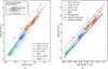 |
Fig. 6 Correlation between cloud size and mass, with the size computed in two different ways. In panel a, the size is defined as the average between the three half-axis of the approximating ellipse, as determined by the structure algorithm. In panel b, the size is computed as the cubic root of the volume. Each dot represents one cloud. The contour lines show a kernel density estimate of the distribution. Starting from the innermost line, approximately 10, 30, 50, and 70% of the distribution lie within the respective contours. The symbols highlight the example clouds from Fig. 2. The grey line in panel a indicates a slope of 3. The solid and dotted line in panel b are iso-density lines for the detection and saddle threshold respectively, as defined in Sec. 2.1 and Appendix A. Their slopes are 3. |
3.2.1 Relation between the number of dimensions and the M-R slope
In Table 2 we list some of the recent mass-size relation slopes obtained from observed cloud catalogues. Both CO and dust extinction studies report mass-size relations with an exponent of about 2 when cloud properties are obtained from projections on the sky. This suggests a constant surface density for clouds (Larson 1981; Lada & Dame 2020). Some studies report a slightly steeper slope, but Ballesteros-Paredes et al. (2019) demonstrated that this is likely an effect of overlapping clouds. Interestingly, when cloud properties are calculated from 3D data, that is the radius from the volume and the mass from the volume density, a scaling relation of M ∝ R3 is obtained, in line with the global relation established in our simulations. Cahlon et al. (2024) investigated exactly the effect of projection on the mass-size relation in their study of clouds extracted from 3D dust maps. They obtained M ∝ R2.9 for 3D clouds but recovered a scaling of M ∝ R2.1 for projected clouds, in agreement with the classical observed relation. This effect was predicted by theory (Ballesteros-Paredes & Mac Low 2002; Ballesteros-Paredes et al. 2012, 2019) and previous analysis of hydrodynamics simulations (Shetty et al. 2010). These works indicate that the slope is determined by the way the size is measured and the underlying number of dimensions. Using the area results in a slope of 2 while using the volume results in a slope of 3. We note that clouds are thought to be fractal in nature (Falgarone et al. 1991; Elmegreen & Falgarone 1996; Elmegreen & Elmegreen 2001) and thus in principle neither of these methods uses a good approximation for the shape. This behaviour is due to the cloud mass being dominated by low density, volume-filling material. This can be seen clearly in the 3D visualisations of our extracted clouds (Fig. 3). This makes the mass sensitive to how the cloud boundaries are defined which relates to the shape. We thus can expect the mass–size relation to change when studying denser structures, such as dense clumps, for which this condition may no longer hold. The LS simulations do contain a the population of small objects which have been stripped of their envelope. Interestingly, they indeed follows a relation which is shallower than 3, as can be seen in Fig. 6a.
Compilation of observational studies, with summary of their underlying data used to produce the molecular cloud catalogue, and their reported mass-size relation.
3.2.2 Normalisation of M-R relation
When M = AR2 the normalisation A provides a roughly constant surface density for clouds, or alternatively a constant average volume density when M = AR3. Lada & Dame (2020) reported a systematic shift of the M-R relation to higher surface densities when clouds have been extracted from dust extinction versus 12CO, in other words the normalisation of the relation is different for different tracers. In fact, for any area in the sky the mass derived from CO is lower than the mass derived from cold dust. Small differences can also be observed between results derived from 12CO and 13CO (Benedettini et al. 2021). This discrepancy could be (partially) due to optical depth effects, which can be severe for 12CO as mentioned already in Sec. 2.4. If the mass is mainly set by the low density material in the cloud envelop rather than the dense cores and filaments, the effect of optical depth on the mass determination should be limited. In this case, the normalisation is set by the density threshold of the cloud extraction algorithm or the equivalent sensitivity limit of the observations, as we concluded from Fig. 6b. The threshold sets a characteristic average density or column density which is a few times larger than the threshold value. Ballesteros-Paredes et al. (2012) demonstrate that this is due to the power-law density PDF of clouds. The amount of mass within a certain density bin decreases rapidly with increasing density. The cumulative mass above a certain density threshold is thus quite sensitive to where you make the cut in the PDF. This has indeed been demonstrated in observations (Lombardi et al. 2010; Beaumont et al. 2012).
3.3 Cloud shapes
We characterise the shape of a cloud by considering the ratio of the half-axes a ≤ b ≤ c of the ellipsoid approximation of the cloud. We compute them from the matrix of inertia of the cloud, assuming the cloud is an ellipsoid with an uniform density (see Eq. (A.5)). The ratio of the shortest half-axis a to the longest c defines how spherical the cloud is, and is called the sphericity. The ratio b/c tells us whether the cloud is oblate, that is pancake-shaped or disk-shaped (a ≪ b ~ c) or prolate, that is filamentary shaped (a ~ b ≪ c). This is illustrated in Fig. 7a where we apply the shape categorisation from van der Wel et al. (2014). We remark that, as we already discussed in Sec. 2.3, the 3D cloud structures are very complex, and the ellipsoidal approximation fails to account for the very different shapes that clouds can actually have. However they are a useful simplification to obtain the extents of the clouds and help classifying them.
3.3.1 Comparison of the typical shapes between simulations
In Fig. 7 we compare the distributions of the shape quantities, which are very similar for all the simulations, except for Ramses-F20. The typical sphericity of the clouds is around 0.35 with values ranging from 0.05 to 0.8, and the middle half-axis is typically equal to 0.55 times the large one. This corresponds to rather prolate structures, such as filament hubs, bent filaments, merging disks and compound structures, or unresolved blobs. We verified that this similarity between all the simulations is not an artefact caused by the cloud finding algorithm: HOP is indeed able to extract objects with largely varying shapes (see Appendix A.7). If we look in more detail, we note that filaments, defined as structures with a ≈ b ≪ c, are common as can be seen in bottom left corner of the diagrams in Fig. 7a. In contrast, spherical clouds are rare as indicated by the emptiness in the top right corner of the diagrams. This indicates that most of the structures are connected with their environment, the filamentary ISM. Oblate disk or sheet shaped structures, that is structures with a ≪ b ≈ c, are also very rare. Ramses-F20 shows a clear excess of them compared to the other simulations. The presence of such disk-like structures is most likely linked with a lack of resolution that prevents further collapse in these regions as already discussed in the previous sections.
Overall, while there is some variety in sphericity within cloud populations, the different simulations feature very similar distributions of the shape parameter. Since here the shape of the clouds is approximated to match an ellipsoid, we can conclude that the global proportions of the clouds are not affected by the details of the physics and the geometry of the simulations. More elaborate measures, such as the fractal index, may provide more insights on the detailed structure of the cloud. This is however beyond the scope of this work.
3.3.2 Discussion of example clouds
To aid with the interpretation of the shape diagnostics and to improve our intuition, we discuss here the shapes of the example clouds displayed in Fig. 2. We start with the clouds extracted from the galaxies Ramses-F20 (fourth row) and M51 (third row) which are generally most massive and illustrate some extreme shapes, before moving to those extracted from the stratified boxes LS (second row) and SILCC (first row) which have properties that are more representative for the entire sample.
The most massive example for each galaxy (left panels, and indicated as a flat vertical diamond in the scatter plots) is a spurious disk with spiral arm pattern. These are amongst the most massive clouds found in their respective simulation. Their disklike shape is reflected by the shape measures: the Ramses-F20 cloud has a/c as low as 0.1 with b/c ≈ 0.75, while the M51 cloud is a little thicker with a/c ≈ 0.2 and b/c ≈ 0.95. This indeed classifies their shape as disky in Fig. 7a. Both these examples have a velocity dispersion high above the global relation due to ordered rotation.
Next, we take the second and third examples of each galaxy simulations, resulting in a collection of four clouds with comparable mass but a variety of shapes. The Ramses-F20 cloud indicated by a triangle appears very isolated and has a smooth appearance with a density gradient towards the centre. It is an categorised as an oblate spheroid with a/c ≈ 0.3 and b/c ≈ 0.85. The second example from M51 looks completely different. It consists of a filament hub system where one major filament is perpendicular to the other. The ellipsoidal shape approximation clearly breaks down in this case. While a/c is indeed very low, b/c ≈ 0.55. This inflates the average size which is almost four times larger than the smooth compact Ramses-F20 cloud of the same mass. This illustrates how the shape alters the mass-size relation in Fig. 6a. If, on the other hand, we estimate the size as the cubic root of the volume, both clouds appear very similar (see Fig. 6b). The third example from each galaxy is a filament which is connected to a larger filament network. The example from M51 is one of the purest filaments in our entire collection with very low a/c and b/c. The Ramses-F20 filament is somewhat thicker with a/c ≈ 0.15 and b/c ≈ 0.25. Both of these seem to be very normal clouds when placed on the mass-size (cf. Fig 6a) and size-velocity dispersion relation (cf. Fig. 9, which will be discussed in Sec. 4.1).
The final example for each galaxy features a small round cloud. For Ramses-F20 this is one of the smallest clouds recovered in this simulation. With a/c ≈ 0.75 and b/c ≈ 0.95 it is also one of the most spherical objects in the entire collection. We note that these are also the least resolved clouds, in which further substructure is subsequently harder to resolve. Extreme non-spherical shapes are therefore less likely to be driven from a natural cascade of turbulent motions.
The example clouds from the stratified box simulations have less extreme shapes. We see that clouds are shaped by a network of connecting filaments, which generally do not align, resulting in the range of a/c and b/c values shown in Fig. 7b. Of note is the fourth example of the LS runs: a comma shapes clump which has been stripped of its low density envelope, making it lie above both versions of the mass-size relation. Generally, a similar argument applies here for the resolution limit and the shape of the cloud. However, this effect is less severe compared to the two disk simulations for two reasons. First, in these simulations we find overall better resolved feedback physics and consequently better resolved turbulent motions. Second, the higher resolution and the overall lower masses for the clouds allows for a stronger impact of sudden external perturbations such as strong shock fronts, which might reshape the cloud to non-spherical objects.
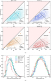 |
Fig. 7 General shapes of the clouds within the simulations. Panel a: relation between the ratio of the middle half-axis over the largest b/c and the ratio of the smallest half-axis over the largest a/c assuming clouds have a ellipsoidal shape. The characterisation of the shape the one used in van der Wel et al. (2014). The contour lines and symbols are the same as in Fig. 6a. Panel b: marginal distributions of the ratio of the ellipsoidal half-axes of the clouds between the simulations. |
3.3.3 Dependence of shape on size
From the examples discussed above, we might have gotten the impression that small clouds tend to be spherical. This is however not generally true. Figure 8a shows the relation between the sphericity of a cloud and the typical size defined as the cubic root of the volume. We do not use the average size defined in the beginning of this section to avoid introducing any spurious correlation. For all the stratified box simulations, the distribution stays unchanged for all size bins between 1 and 10 parsec. Interestingly, the mean value of the sphericity decreases when the typical size is around 10 pc. A possible interpretation is that large clouds are more likely to undergo external influence, like turbulent motion. Also, they may be younger objects which kept their initial filamentary shape. It may also be just a resolution effect: clouds with a smaller number of cells tend to be more spherical while a higher number of cells allows for more complex shapes. However, Fig. 8b demonstrates that this is not the case: expect for M51, the distribution of the sphericity does not vary much when looking at objects with a different number of cells. Although clouds with very high sphericity are found only when the number of cells is small, they represent only a tiny fraction of the sphericity distribution, which is well sampled for all cell numbers. In the stratified box simulations, there is no significant decrease of the sphericity with an increase of the number of cells. Such a trend is however visible for the less resolved full-galaxy simulations, especially in M51, and in a lesser extent in Ramses-F20.
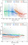 |
Fig. 8 Sphericity as a function of structure size, computed from the volume (a) or the number of cells (b). The solid line depicts the mean in a logarithmic bin of size, and is computed only if the bin contains at least 100 clouds. Contour lines and symbols are as in Fig. 6a. |
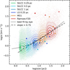 |
Fig. 9 Cloud velocity dispersion as a function of the size. The dashed line illustrates a scaling of σ with size R0.75 while the curved solid line illustrates the trend of the centroids of each distributions. The contour lines and symbols are the same as in Fig. 6. |
3.3.4 Shapes in observations
In observations, clouds can be approximated by the 2D equivalent of our ellipsoids, ellipses, since they appear as 2D projections on the sky. In this case a minor and major axis is reported and their ratio incorporates the shape. Since there is no information about the size along the line of sight2, it is unclear whether this ratio is more comparable to our a/c or b/c. If we assume that clouds are randomly oriented, then the observed value would represent an average of a/c, b/c and a/b. Taking the geometric mean of the peak value of the distribution for each of these ratios results in (0.35 × 0.55 × 0.65)1/3 = 0.5. The SEDIGISM (Duarte-Cabral et al. 2021), FQS (Benedettini et al. 2020, 2021) and Miville-Deschênes et al. (2017) catalogues provide the two projected sizes for their objects. Their ratio is typically between 0.2 and 0.8 and the distribution peaks between 0.4 and 0.6. For SEDIGISM and FQS, which have extracted clouds in a similar way, the peak is closer to 0.45, in line with the averaged value we find. For the Miville-Deschênes et al. (2017) catalogue, where the sizes were derived differently, the peak is more towards 0.6, close to what we find for b/c. As a test, we can also project our 3D clouds on a 2D plane and calculate the projected size as a geometric average of the major and minor axis of an approximate ellipse, equivalently to our ellipsoid approximations. This results indeed in a broad distribution with a peak around 0.5. Thus, while an accurate comparison for the shape seems rather impossible, we can confidently say that simulation and observations agree that clouds are typically elongated.
4 Analysis of internal properties of clouds
4.1 Size – velocity dispersion relation
The velocity dispersion is also correlated with the cloud size (Hennebelle & Falgarone 2012; Heyer & Dame 2015). This is the so-called Larson relation (Larson 1981), which is considered a signature of the turbulent cascade (Elmegreen & Scalo 2004). Indeed, for compressible supersonic turbulence a scaling of σ ∝ lβ with β between 1/3 and 1/2 is expected (Kritsuk et al. 2007). Observationally, a large scatter is found in the line-width – size relation. Some studies agree with this theoretically predicted slope (Solomon et al. 1987; Kauffmann et al. 2013), but some find steeper slopes (Miville-Deschênes et al. 2017), which shows that the relation may not be as universal as generally believed.
The velocity dispersion of our extracted clouds has been calculated as a mass averaged quantity (see Eq. (A.8)). The size is derived from the ellipsoid approximation as mentioned in the previous section and detailed in Appendix A.
4.1.1 Continuous relation across simulations
Figure 9 shows the cloud internal velocity dispersion as a function of their size for all simulations. The dashed line illustrates the power-law scaling with 0.75. In addition, we show the actual scaling with the solid line that passes through the innermost contour line of all sets of clouds. Despite the overall large scatter, the majority of the clouds (inner contours) form a continuous distribution across the set of simulations.
We note that the distribution is bounded towards the low-σ end approximately half an order of magnitude below the dashed line. There are hardly any clouds with a lower velocity dispersion. This is in line with the turbulent motions in the gas and the gravitational collapse in massive clouds, which increases the internal velocity dispersion. In contrast, there is no clear cut at the high-σ end of the distribution. In particular for the small clouds (mainly the SILCC simulations) and the clouds from galaxy Ramses-F20, there is a population of clouds with strong internal motions. Overall, for small clouds the internal velocity dispersion is significantly enhanced compared to the indicated power-law scaling – in particular the inner contours of the cloud distributions from the SILCC simulations.
4.1.2 Observed scaling and break in the power law
Canonically, the size-velocity dispersion relation has been described by a power law with slope 0.5. However, the simulation results indicate that the relation is somewhat more complex, in a sense that it in fact does not follow a simple power law. In Fig. 10 we compare our results to the catalogues from Miville-Deschênes et al. (2017) and Benedettini et al. (2020). We keep in mind that the velocity dispersion is determined in a very different way in the simulations compared to the observations. Nonetheless, the observations of Benedettini et al. (2020) show a flattening of the relation below sizes of about 5 pc, with the velocity dispersion saturating at a value of about 1.4 km s−1 (when converted from 1D to 3D dispersion assuming isotropy), in agreement with the global trend found in the simulations. The bulk of the SILCC clouds even seem to slightly underestimate the small scale velocity dispersion. This is not surprising since the simulations do not take into account processes that inject turbulence at small scales, such as stellar winds and jets. Another possible interpretation is that the observations are biased towards gravitationally collapsing objects. The outermost contour of LS, simulations which preferentially resolve the collapsing objects within them as discussed in Sec. 5.1, indeed seems to follow the observations.
While we do recover a global power-law behaviour for large clouds, the slope from the simulations is somewhat steeper, that is to say about 0.75, compared to the already fairly steep 0.6 found by Miville-Deschênes et al. (2017). For large clouds, the extraction from the simulations measures on average a slightly larger velocity dispersion than the observations from Miville-Deschênes et al. (2017) for a certain size bin. The simulation results may overestimate the dispersion due to several reasons. We calculate the dispersion in a somewhat naive way which does not take into account organised motions within the cloud such as rotation, radial gravitational inflow or colliding flows. These are not forms of turbulence and should thus be accounted for when one wants to quantify the turbulence velocity dispersion. An alternative interpretation is a systematically different size estimate, such that the sizes for the observed clouds are larger than the ones from the simulations. This is in fact a plausible explanation given that clouds are overlapping along the line of sight as illustrated in the simulations in Fig. 2 and cloud blending can be sever especially at large distances.
What the simulations and observations do agree on is the large scatter. For a specific size, the estimated velocity dispersion can vary by an order of magnitude.
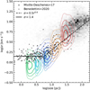 |
Fig. 10 Comparison of the 3D size-velocity dispersion relation found in the simulation with several cloud catalogues from observations. Coloured contours are as in Fig. 6. Observational data feature only the 1D line-of-sight velocity dispersion, which was here multiplied by |
![Mathematical equation: $\[\sqrt{3}\]$](/articles/aa/full_html/2024/06/aa48983-23/aa48983-23-eq4.png)
4.1.3 Origin of high velocity dispersion clouds
A high velocity dispersion can have several origins, among which externally driven turbulence and self-gravitating collapse are two prominent examples. In the case of gravitational collapse the clouds are likely to be embedded in a dense environment with cold temperatures. In the case of externally driven turbulence, that propagates into the clouds, the gas temperature can be enhanced if the external turbulence is driven by SN feedback and penetrates into the clouds from the warm or hot phase of the ISM.
In order to identify the mechanism at work for the small clouds we investigate the locations of the clouds in Fig. 1a for simulation SILCC-0.5pc. The corresponding SILCC simulations with higher and lower resolution are very similar. The grey-scale colour-map shows the gas column density. The clouds identified by HOP are over-plotted with the colour indicating the internal velocity dispersion. There is no clear correlation between the position of the clouds in the global gas structure and their velocity dispersion. However, the lowest values of σ are found for points that tend to be more embedded in large gas structures. On the other hand, clouds closer to the low-density bubbles that have formed as a result of SN feedback have intermediate to high velocity dispersions. We further illustrate this in Fig. 11, where we show slices of density, temperature and velocity at the positions of two example clouds with high velocity dispersion, both located at the interface between cold gas and a hot bubble.
A more systematic analysis is shown in Fig. 12 for the clouds in SILCC-0.5 pc (again, different resolutions do not differ) for which we investigate a spherical region around the clouds with a radius twice the average size obtained from the cloud algorithm. Both panels show scatter plots of σ as a function of cloud mass. In the left-hand panel the clouds are colour coded by the mass-weighted temperature in the investigated volume. The right-hand counterpart shows the fraction of molecular gas in in the volume. We note that the clouds with higher velocity dispersion clearly show enhanced temperatures and lower fractions of molecular hydrogen. This illustrates that the clouds which are surrounded by warm or hot gas have statistically higher velocity dispersions. In the SILCC setups analysed here, the only source of hot turbulent gas are SN explosions. We therefore conclude that the enhanced motions in the clouds are due to SN-driven turbulence. We note that these warm clouds with low H2 fractions would also contain little CO and as a result could be missing from classical observational catalogues.
In the full galaxy simulations RAMSES−F20 and M51, there is also a population of clouds with high-velocity dispersion, but the mechanisms at play are different. Most of these clouds, which are also very large, are rotating disks, which explains the high velocity dispersion. The existence of such disks with radius of around 100 pc is a spurious effect of the lack of resolution in these regions, as we would expect these structures to collapse and fragment into smaller objects.
4.2 Virial parameter
In addition to the size-velocity dispersion relationship, we also compute the virial parameter αvir. for the clouds in our simulations, using the definition given in Eq. (1). The results are shown in Fig. 13. We can see immediately that αvir· has a clear dependence on mass: αvir·∝ M−n, with n = 0.4. In other words, lower mass clouds on average have much larger values of αvir than higher mass clouds. Therefore, although there is generally good agreement between the simulations for the mass ranges where their cloud populations overlap, the mean value of αvir differs significantly between different simulations. This demonstrates that care must be taken when using simulations to draw conclusions about the gravitational boundedness of interstellar clouds3. Different simulations may lead to very different conclusions about whether or not clouds are bound if they differ significantly in terms of resolution or box size, and hence do not probe the same portion of the cloud mass hierarchy.
We also see that there is substantial scatter in the value of αvir that we recover for any given cloud mass. For the majority of clouds, the value of αvir varies by about one order of magnitude for a specific mass range, but in a small fraction of clouds the value of αvir can be as much as 100 times the typical value for a given mass. At fixed mass, αvir depends only on the cloud size R and velocity dispersion σ. However, we have already seen that at fixed M, the cloud size varies by only around a factor of two in most cases (see Fig. 6), and so the majority of this scatter must be driven by variations in the velocity dispersion. This conclusion is consistent with what we have already found for the velocity dispersion-size relation: for most clouds, σ varies by around a factor of three at fixed cloud size (see Fig. 9), corresponding to an order of magnitude variation in αvir if we keep M and R fixed, but for a small number of clouds we find much larger values for σ and hence for αvir. It hence seems likely that the factors responsible for the outliers in the αvir−M distribution are the same as those responsible for the outliers in the σ−R distribution, namely stellar feedback at low cloud masses and lack of resolution leading to artificial rotational support at high cloud masses (see Sec. 4.1).
Finally, it is interesting to compare the αvir−M relation that we recover from the simulations with the one measured for real interstellar clouds. As is clear from the compilation of data in Chevance et al. (2023), different galactic and extra-galactic cloud surveys recover a similar scaling αvir ∝ M−05 at low cloud masses, but with a normalisation that varies between surveys by up to an order of magnitude. These results are also in agreement with observations of the densest regions within molecular clouds, parsec-scales structures called clumps. Several surveys dedicated to the study of the dynamics at these scales using high density tracers (e.g. NH3 or N2H+) report a scaling αvir ∝ M−0.5 (Urquhart et al. 2018; Traficante et al. 2018a). Although the behaviour of this scaling relationship on the scale of individual clumps is debated (Kauffmann et al. 2013; Traficante et al. 2018b; Singh et al. 2021), it is remarkable to note that the average slope observed using high-density tracers is in overall agreement with CO cloud surveys and with the results of the simulations in this work. In fact, overall, the range of values found in observations are in good agreement with the location of most of our simulated clouds in the αvir−M plane (see grey crosses in Fig. 13), but the small population of clouds we recover that have very high virial parameters do not appear to have observational counterparts in CO-based surveys. This may simply reflect the fact that many of these clouds have been strongly affected by stellar feedback and hence would in reality have little molecular gas associated with them. The slope that we recover for the αvir−M relation also agrees well with the observed slope: our best fit value is slightly flatter than that found in the observations, but as we show in Fig. 13, a slope of −0.5 also provides a relatively good fit to the data from all of the simulations apart from Ramses-F20. However, we caution that this agreement may be strongly influenced by selection effects. Observationally, clouds with an integrated intensity close to the detection limit of a survey and a velocity dispersion close to the velocity resolution will all have approximately the same molecular gas surface density, implying that for these clouds, R ∝ M0.5. For fixed σ, this then yields αvir ∝ M−0.5. A similar combination of limited sensitivity and velocity resolution may also explain the similarity between the scaling relationships recovered for dense clumps and for molecular clouds. Our population of simulated clouds does not suffer from this selection effect, but the fact that, as previously discussed, HOP selects clouds with a relatively narrow range of mean densities also strongly biases us against finding clouds with low αvir at low M.
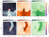 |
Fig. 11 Two examples showing the positions of the clouds with their respective density (left), temperature (middle), and velocity environment (right). In both cases the clouds are located at the edge between cold gas and a hot SN-driven bubble. The resulting high velocity dispersion is thus due to SN-driven turbulence that mixes hot gas into the clouds rather than by gravitational collapse. |
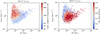 |
Fig. 12 Scatter plot of the velocity distribution as a function of cloud mass for simulation SILCC-0.5pc. Left: colours indicate the mass-weighted temperature in a sphere around the centre of the HOP cloud with a radius corresponding to twice the average size of the HOP cloud. Right: colours indicate the molecular fraction in the surrounding sphere. |
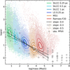 |
Fig. 13 Virial parameter as a function of cloud mass for all simulations. Coloured contour lines are the same as in Fig. 6. Over-plotted are the slope of the scaling (thick grey line), as well as the observational data compiled for the PPVII review (Chevance et al. 2023). |
4.3 Thermal state
In order to quantify the thermal state of the gas in the clouds identified in the different simulations, we have computed the mean temperature T for each cloud. We compare the distributions of mass-weighted average cloud temperatures in Fig. 14, where we show results from the LS, M51 and Ramses-F20 simulations, plus a representative example from the SILCC simulations.
From the figure, we see that there are some significant differences in the average cloud temperatures in the simulations. All of the simulations show a clear peak at low temperatures, but they do not agree on the location of this peak: it is found at T ~ 25 K in the M51 simulation, T ~ 100 K in the LS and Ramses-F20 simulations, and at T ~ 60 K in the SILCC simulation. This appears to be primarily due to a difference in the effectiveness of photoelectric heating in the various simulations. In the LS and Ramses-F20 simulations, the photoelectric heating rate is computed assuming no local attenuation of the interstellar radiation field. Since much of the cloud mass is located at a density close to the HOP threshold density, we would therefore expect the temperature of this gas to be comparable to that of a patch of unshielded ISM with a density n ~ 30 cm−3. For an interstellar radiation field strength comparable to the solar neighbourhood value, this is T ~ 100 K (Wolfire et al. 2003), in good agreement with the low T peak we find in these simulations. In the SILCC and M51 simulations, we attempt to account approximately for the effects of local attenuation using the TreeCol algorithm (Clark et al. 2012; Wünsch et al. 2018). The clouds formed in these simulations therefore feel an effective photoelectric heating rate that is lower than in the Ramses simulations, and hence have lower characteristic temperatures. Finally, the difference between the SILCC and M51 simulations stems from the fact that the two populations of clouds have similar mean densities but different sizes (see Fig. 6). The M51 clouds therefore have mean surface densities that are a factor of a few larger than the clouds in the SILCC 0.5 pc simulation, giving them higher mean extinctions and hence lower photoelectric heating rates.
The temperature distributions shown in Fig. 14 also differ significantly at the high T end. In the SILCC and M51 simulations, very few clouds have average temperatures as high as 1000 K, while in the LS and Ramses-F20 simulations, there is a substantial population of clouds with high mean temperatures, extending up to T ~ 104 K. This behaviour is a consequence of differences in the way that stellar feedback is modelled in the simulations. In the LS simulations, the effects of photo-ionisation feedback are included. As HOP identifies clouds based purely on their density structure, without reference to their chemical composition, it therefore extracts some clouds that have been partially or totally photo-ionised, but that have not yet expanded sufficiently to bring their mean density below the cloud identification density threshold. The peak in the temperature distribution at T ~ 104 K corresponds to fully ionised clouds, while clouds with temperatures between a few 100 K and 104 K have only been partially ionised, and hence have a mean temperature that is intermediate between the low temperature of their neutral portion and the ~ 104 K temperature of their ionised portion. In the Ramses-F20 simulations, ionising radiation is not explicitly followed with a radiative transfer code, but is accounted for approximately by maintaining the temperature of the gas in any grid cells containing massive stars at 104 K (Kretschmer & Teyssier 2020). Therefore, the mean cloud temperature in this simulation depends on the number of cells in the cloud that contain massive stars, with the highest mean temperatures corresponding to clouds in which most or all of the grid cells are affected by the local heating. Finally, we do not see this population of warm clouds in the SILCC or M51 simulations because these simulations do not include any treatment of photoionisation feedback. In principle, SN feedback could produce a similar effect if we were to happen to identify a cloud in which a supernova had just exploded, but in practice, clouds in which SNe have exploded are rapidly disrupted and so the chances of this occurring are relatively small. That said, we do find exactly one example of such a cloud in the M51 simulation, with mean temperature of ~3 × 10⁵ K, visible on the far right in Fig. 14.
The fact that we see such clear differences between the distributions of cloud-averaged temperatures in the different simulations indicates that this is a quantity that is very sensitive to how we chose to model the thermal physics of the ISM and the impact of stellar feedback in our simulations. However, the fact that many of the other cloud properties that we have examined agree well between different simulations demonstrates that even large differences in cloud temperatures have a relative small effect on the other properties of the clouds, consistent with the idea that these are shaped more strongly by turbulence than by thermal pressure.
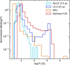 |
Fig. 14 Distribution of cloud-averaged temperatures. |
5 Discussion
We already discussed individual results extensively in their corresponding sections. Here we address further the issue of resolution and explore the dependence on the cloud extraction algorithm.
5.1 Resolution dependence
The influence of the resolution of the simulation on the extracted cloud population is most easily seen in the cloud mass spectrum. We already discussed in Sec. 3 that the peak of the mass spectrum depends on the resolution. However, if we normalise according to the number of clouds per unit area, we see that all simulations follow the same distribution. The effect of increasing the resolution is thus purely to be able to resolve an additional population of smaller clouds; the absolute number of large clouds remains the same. When the resolution is low, it is possible that some clouds become blended. In this case one would expect to find more massive objects. The universality of the obtained mass spectrum slope for simulations with different resolutions shows that this is not an issue, at least when structures are extracted with the algorithm used in this work. Some small clouds may be counted as being part of a larger cloud, but since their mass and size are negligible compared to the properties of the larger cloud, this does not change the statistics.
We also saw that the shape of the low-mass part of the mass spectrum depends on the simulation code. The LS and Ramses-F20 simulations show a gradual decline towards smaller and smaller masses, while the SILCC runs show a sharp cut-off at the resolution limit. The differences between the grid code simulations run with RAMSES (LS and Ramses-F20) and FLASH (SILCC) are related to the different refinement strategies used in the two codes. While both codes use refinement criteria that trigger grid refinement in dense regions, the SILCC simulations have block refinement, such that the entire rectangular block of 83 cells around the dense region is also refined in order to keep the grid structure simple. This results in a significant fraction of cells having high refinement levels, as illustrated in Table 3, which in turn allows for well-resolved turbulence inside the majority of the domain. By contrast, the RAMSES runs were refined in a very localised fashion, and hence although they resolve gravitationally collapsing structures well, they capture less of the turbulent cascade to small spatial scales that occurs in the more diffuse ISM. This results in them missing a population of small structures created by turbulence.
To verify this, we compare the results of two RAMSES test simulations of the stratified box type which apply different refinement criteria. The first simulation uses a targeted refinement strategy, similar to the one used in the LS simulations listed in Table 1, which focusses on following the gravitational collapse of dense objects. This is done by requiring the local Jeans length and mass, which vary with scale, to be resolved by a certain number of cells. The second simulation has more abundant refinement, meaning that refinement is triggered more frequently in lower density gas. This is achieved by setting a uniform limit on the mass that can be contained in a cell. This results in many more cells and thus significantly longer computation time. Figure 15 compares the mass spectra of the clouds extracted in these two runs. We see that the abundant strategy is able to resolve many more low-mass structures and has a mass spectrum with a shape comparable to what we found for the SILCC runs. The run with the selective refinement strategy has a peak at larger values and a low-mass tail which becomes more prominent over time as gravitational collapsing structures develop. This test indeed confirms that the difference in refinement strategy results in a different mass spectrum for SILCC and LS.
Number of cells and fractions of cells on each refinement level for the stratified box simulations.
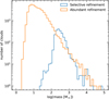 |
Fig. 15 Comparison of the cloud mass spectrum in two RAMSES test simulations with a similar setup to simulation LS using different refinement strategies. |
5.2 Cloud extraction parameters and other algorithms
There are many ways to extract clouds from simulations and the results depend on the implementation and chosen parameters of the extraction algorithm. In Appendix A.4 we test the dependence of the mass spectrum on the chosen parameters of the HOP algorithm. Notably, the saddle merging criterion is found to have a significant effect on the slope. If we do not use the saddle merging criterion, the mass spectrum is closer to a log-normal rather than having a power-law high-mass tail. Without saddle merging, the mass spectrum will depend strongly on resolution, since resolved substructures will be counted as individual objects. When enabling saddle merging, the slope of the power-law decreases with decreasing merging density value. When merging everything that touches, using the most aggressive merging strategy possible with ρsaddle = ρthreshold, the mass spectrum is significantly shallower than the value of ρsaddle = 10 ρthreshold we adopted in this work. The majority of small objects are absorbed into large cloud complexes.
The mechanics of HOP with the most aggressive saddle merging is similar to how the friends-of-friends (FOF) algorithm operates. For particle simulations, FOF dictates that two particles with a density above the required threshold belong to the same group if they are within a specified distance from one another, typically taken to be some fixed fraction of the mean inter-particle separation. For grid simulations, one typically requires the cells to be neighbours. Iffrig & Hennebelle (2017) used FOF to identify clouds in kpc-sized boxes similar to the LS simulations used in this work. They applied a slightly higher density threshold of 50 cm−3 and find that the slope of the mass spectrum depends on the strength of the magnetic field. Without magnetic field the fitted slope is around −1 or slightly steeper. For an initial field of 3–6 μG, comparable to the field strengths used in the stratified box simulations analysed in this work, they obtain shallower slopes, about −0.7 to −0.8. These values are shallower than what we recovered with HOP, in line with the difference observed when changing the saddle merge criterion.
The mass-size relation is also affected. Iffrig & Hennebelle (2017) report that their results are in line with the observed slope of 2.36, somewhat shallower than the general trend of −3 we found in Sec. 3. In Fig. 16, we see that we indeed find a shallower mass-size relation when extracting the clouds with a FOF-like algorithm. Small objects are merged into larger ones, tilting the slope.
Another approach is to use dendograms, which describe the hierarchy of structures in the form of a tree. Tress et al. (2021) extracted clouds from their M51 galaxy, that we also use in the comparison in this work, using SCIMES (Colombo et al. 2015). This stands for Spectral Clustering for Interstellar Molecular Emission Segmentation and is a technique mainly used in observations. It is based on the cluster analysis of dendrograms of 3D (in the PPV or PPP space) data cubes that performs particularly well for the identification of large structures such as the molecular clouds in spectroscopical observations of large fields in the Milky Way (e.g. Colombo et al. 2015; Schuller et al. 2017; Benedettini et al. 2020). SCIMES considers the dendrogram tree of the 3D structures in the data cube (using the implementation of Rosolowsky et al. 2008 for astronomical data-sets) and groups different leaves together into ‘clusters’ of leaves, based on one or more criteria. We note that the parameters of the extraction in Tress et al. (2021) are different than ours, which means that we should not over-interpret details in the numbers. They use the extraction based on molecular hydrogen with a threshold number density of ![Mathematical equation: $\[n_{\mathrm{H}_2, \min }=1 \mathrm{~cm}^{-3}\]$](/articles/aa/full_html/2024/06/aa48983-23/aa48983-23-eq5.png) . This does not simply translate into a total number density as shown in detail in e.g. Seifried et al. (2017) for the same chemical network. Furthermore, the dendrogram methods works on a grid-based data set, which requires the Arepo cells to be mapped onto a (locally) uniform grid. Whereas, this is not expected to yield systematically different results if the resolution is high enough, it might easily shape the outliers in the distributions. Nonetheless, many of the extracted cloud properties are well in line with our values. The bulk of the cloud masses extracted in (Tress et al. 2021) broadly range from 103−105 M⊙, slightly higher but well within the scatter given the differences for the parameters. The sizes of the clouds peak at ~ 10 pc, which is close to our sizes. Both the mass-size relation and the size-velocity dispersion relation are in line with the trends found in this work. Furthermore, the virial parameters are very similar (αvir ~ 10) as well as their flat scaling with mass. This illustrates that different cloud extraction methods do not always have to disagree.
. This does not simply translate into a total number density as shown in detail in e.g. Seifried et al. (2017) for the same chemical network. Furthermore, the dendrogram methods works on a grid-based data set, which requires the Arepo cells to be mapped onto a (locally) uniform grid. Whereas, this is not expected to yield systematically different results if the resolution is high enough, it might easily shape the outliers in the distributions. Nonetheless, many of the extracted cloud properties are well in line with our values. The bulk of the cloud masses extracted in (Tress et al. 2021) broadly range from 103−105 M⊙, slightly higher but well within the scatter given the differences for the parameters. The sizes of the clouds peak at ~ 10 pc, which is close to our sizes. Both the mass-size relation and the size-velocity dispersion relation are in line with the trends found in this work. Furthermore, the virial parameters are very similar (αvir ~ 10) as well as their flat scaling with mass. This illustrates that different cloud extraction methods do not always have to disagree.
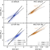 |
Fig. 16 Mass-size relation for the LS stratified boxes and M51 galaxy when using our default HOP parameters versus FOF-like merge criteria. Coloured contour lines are the same as in Fig. 6a. |
6 Summary and conclusions
In this paper, we extracted clouds from multi-physics ISM simulations using a set of four different types of (M)HD simulations (SILCC, Girichidis 2021; LS, Colman et al. 2022; M51, Tress et al. 2021; Ramses-F20, Brucy 2022). The set covers a large range in spatial scales from 0.25 pc for the smallest cells in patches of the ISM up to a full galactic disks with a diameter of 30 kpc. Furthermore, the simulations were performed using different codes (FLASH, RAMSES and AREPO) with distinctive numerical techniques and physics ingredients of varying complexity. For all data sets, we used a standardised 3D density-based extraction method build around the HOP algorithm.
We find that many properties of the extracted clouds follow robust trends across scales and very smooth transitions between the different simulations despite the vast differences in resolution, physics included, size of the box and setup geometry. In particular the relation between mass, size, shape and velocity dispersion (see Sects. 3 and 4.1 and Figs. 4, 6, 7 and 9) show remarkably consistent scaling properties. This suggests some universality of these relations, and that gravity and turbulence, which are equally present in all simulations, are the key drivers of (molecular) cloud properties.
More specifically, our results can be summarised as follows:
The geometry of the extracted clouds ranges from roundish object to complex filamentary networks. Consequently, the precise shape is only poorly represented by simple quantities such as the sphericity or the triaxiality. However these quantities, computed from a ellipsoidal approximation of the shape of the clouds, are useful to characterise their 3D extents. The sphericity and triaxiality are very consistent across all simulations and across the number of cells per cloud within each simulation with a sphericity of 0.25 − 0.4. This is not an artefact of the extraction algorithm, which is able to detect all complex shapes from the simulations.
The mass spectra of the clouds follows a remarkably consistent and universal distribution: the normalised number of clouds per unit area of interstellar gas results in a common shape of the high-mass end of the distributions with a slope of dN/d ln M ∝ −1 across 6 orders of magnitude. No scaling of individual simulations was required to match this universal high-mass distribution across the simulations.
The slope of the mass distribution in our simulations agrees with theoretical predictions but differs from other numerical work and observations. We show that this discrepancy can easily originate from the extraction method used.
The low-mass end of the distributions is sensitive to the applied refinement criterion. An aggressive refinement, such as used in SILCC that does not only act on a small volume around collapsing regions, allows for both higher resolution at intermediate densities and a better representation of the turbulent cascade. Consequently, in this case many more structures form in the presence of and driven by turbulent motions. The resulting mass distributions show the universal scaling down to a small multiple of the resolution limit of the simulation. This naturally comes at a much higher numerical cost. The original LS simulations use a more localised refinement, which results in a peak of the mass spectrum at significantly higher masses. However, tests with similarly aggressive refinement show a consistent evolution with SILCC.
The relation between cloud mass and size follows a smooth power law of the form M ∝ R3 across simulations. The normalisation reflects the density threshold used by the extraction algorithm.
The internal velocity dispersion also scales very smoothly across the setups. For the large clouds, the trend is a power law σ ∝ R0.75. For clouds smaller than ~0.5 pc we find a deviation from the power-law scaling towards higher velocity dispersions. The median value for σ seem to asymptotically approach ~0.5 km s−1. A detailed analysis shows that this base level of internal velocity dispersion results from supernova-driven turbulence rather than gravitationally driven collapse. The small (low-mass) clouds with higher σ show a higher mass-weighted temperature and reduced fraction of molecular gas, which is in line with turbulence driving from the hot and warm phases into the clouds.
A comparison with observational catalogues shows a similar trend of a power-law scaling of σ with size and a flat distribution for small clouds with a base level of internal velocity dispersion of approximately 1 km s−1. The scaling for the simulated clouds of σ ∝ R0.75 is steeper compared to the observed scaling of σ ∝ R0.6, which does not necessarily mean an inconsistency in the dynamics of clouds, but could also be related to the differently inferred sizes of the clouds between simulations and observations.
The scaling of the virial parameter αvir with mass agrees well with the αvir ∝ M−0.5 scaling found in observations of both molecular clouds and dense clumps. However, it is difficult to say whether this is a robust physical result or merely a consequence of the selection effects affecting both observational and numerical measurements of αvir.
The mean cloud temperatures do not agree well between simulations, primarily due to differences in the treatment of photoelectric heating and stellar feedback in the different models. However, the good agreement we find in other cloud properties despite this difference in temperatures suggests that the thermal pressure of the gas has only a small influence on these properties.
Care must be taken when comparing mean cloud properties between catalogues, as different simulations (or observations) may trace different parts of a universal cloud hierarchy. Catalogue averages reflect the resolution and volume under study.
The catalogues we produced along with the analysis tools are publicly available in the Galactica database4.
Acknowledgements
We thank the anonymous referee for their useful comments. This project was funded by the European Research Council under ERC Synergy Grant ECOGAL (grant 855130), led by Patrick Hennebelle, Ralf Klessen, Sergio Molinari and Leonardo Testi. The authors acknowledge Interstellar Institute’s program “II6” and the Paris-Saclay University’s Institut Pascal for hosting discussions that nourished the development of the ideas behind this work. The authors gratefully acknowledge computing resources provided by the Ministry of Science, Research and the Arts (MWK) of the State of Baden-Württemberg through bwHPC and the German Science Foundation (DFG) through grants INST 35/1134-1 FUGG and 35/1597-1 FUGG, and they thank for data storage at SDS@hd funded through grants INST 35/1314-1 FUGG and INST 35/1503-1 FUGG. RSK and SCOG furthermore acknowledge financial support from the Heidelberg Cluster of Excellence STRUCTURES in the framework of Germany’s Excellence Strategy (EXC-2181/1 – 390900948), and from the German Ministry for Economic Affairs and Climate Action in project MAINN (funding ID 50OO2206). CRediT author statement (more information about the roles defined by the CRediT system can be found here: https://www.elsevier.com/researcher/author/policies-and-guidelines/credit-author-statement): Tine Colman: Conceptualisation, Software, Formal Analysis, Investigation, Writing – Original Draft. Noé Brucy: Conceptualisation, Formal Analysis, Investigation, Writing – Original Draft, Visualisation, Data Curation. Philipp Girichidis: Conceptualisation, Formal Analysis, Investigation, Writing – Original Draft. Simon C. O. Glover: Conceptualisation, Writing – Original Draft. Milena Benedettini: Resources, Writing – Review & Editing. Juan D. Soler: Writing – Review & Editing. Robin G. Tress: Resources, Writing – Review & Editing. Alessio Traficante: Writing – Review & Editing. Patrick Hennebelle: Conceptualisation, Resources, Writing – Review & Editing, Funding Acquisition. Ralf S. Klessen: Conceptualisation, Writing – Review & Editing, Funding Acquisition. Sergio Molinari: Conceptualisation, Funding Acquisition. Marc-Antoine Miville-Deschênes: Resources, Writing – Review & Editing
Appendix A Structure finding algorithm
The full algorithm, including test setups, can be found in the ecogal_tools repository on gitlab. It is built around the HOP clump finder, as described and implemented by Eisenstein & Hut (1998). Here we give a summary of their implementation, discuss our adaptation and parameter choices for application to hydrodynamics simulations and present some test results.
Appendix A.1 Finding groups around local peaks
First, the list of particles is read from the input file. For this step, we need to provide HOP with the coordinates x, y, and z of each particle or cell5, as well as their mass and density. If we do not have density information, we can ask HOP to calculate it for us by applying a smoothing kernel. However due to grid codes already providing densities and SPH codes possibly using a variety of kernels, we think it more straightforward to leave the density calculation to the user in the case of hydrodynamics simulations. While we typically perform the structure finding on the density field, it can in theory be applied on any field.
A search tree is constructed based on the particle positions to allow for efficient neighbour searching. For each particle, the highest density neighbour among the Nhop closest neighbours (including the particle itself) is identified. We keep the default value of Nhop=16. Eisenstein & Hut (1998) verified that the result is insensitive to this parameter for particle simulations. For grid simulations, a minimum of 7 is required to probe the direct neighbours of a fully refined region. Adopting large value (e.g. 27 which would probe also the diagonal neighbours in a fully refined region) could lead to artificial merging of structures that are separated by cells that are not at the deepest refinement level. The larger Nhop, the larger the computation time.
Next, for each particle we follow the chain of densest neighbours. For the highest density neighbour, we find its own highest density neighbour, then find the highest density neighbour of that particle, etc. We proceed in this way along the chain until we eventually reach a particle that is its own densest neighbour. The particle we started with is then assigned to the group of the final particle. For example, we start at particle A which has a densest neighbour B. We then go to particle B and see that the densest neighbour of B is C. Arriving at C, we see that there is no particle around C that is denser than C, meaning that C is its own densest neighbour. Particle A is then assigned to the group of C. The name ‘hop’ actually refers to this process of hopping between neighbours. The result is a collection of peak patches around local density maxima. The resulting segmentation is outputted to file as an intermediate result, which can be reused later.
To prepare the field for the next step, HOP also investigates the boundaries of the identified structures. For each particle, we check whether any of the closest Nmerge neighbours belongs to a different structure. If this is indeed the case, we found a boundary and its density, called the saddle density, is defined as the average between the particle and the neighbour that is in the other group. For each pair of structures, the highest saddle density is recorded and outputted as an intermediate result. We set Nmerge=8, larger than the default value of 4, to account for the regularity of the neighbour locations in grid codes. When provided with information on the size of the computational domain, HOP accounts for periodic boundaries when determining neighbours.
Appendix A.2 Altering and merging groups
Once HOP has identified all the peak patches, we move to the regrouping phase executed by the REGROUP algorithm (Eisenstein & Hut 1998). This serves to exclude low density particles, to reduce noise and to merge structures according to user specified criteria. For example, a cloud could consist of multiple peaks which are blended together. Or we could have a cell with an unusually high density fluctuation with nothing else around it which should be considered as noise. Four parameters control this phase.
A density threshold rho_thresh is set to allow only cells with a density above this value to be included in structures.
A required peak density rho_peak is set to identify an individual structure, as opposed to noise or low amplitude fluctuations inside another structure.
A maximum allowed saddle density rho_saddle is set to identify an individual structure as opposed to the patch being part of a larger entity.
The structure has to have a minimum number of cells min_cells.
First, all particles which have a density below rho_thresh are removed from peak patches. Usually the value of this parameter is determined by the type of structure we want to obtain. We typically adopt the thresholds 1 cm−3 for cloud complexes, 30 cm−3 for clouds and 1000 cm−3 for clumps. It is important to note that generally these thresholds are arbitrary and that varying them can give interesting additional information. From an observational point of view, we can set the threshold to approximate the point where we can detect a certain tracer, e.g. CO. This, in turn is determined by the chemical species under study and the sensitivity of the detector.
Next, the algorithm merges structures based on the remaining criteria. If the peak density is not sufficient, observations would not pick it up as an individual structure. There are now several possibilities depending on whether it has neighbours or not. If the structure has a neighbour that does qualify as an individual entity and the saddle is above the saddle threshold, the structure is merged with this neighbour. If there are multiple neighbours, the one with the largest saddle density is chosen. When there are no suitable neighbours, the structure does not stand out enough from the background and is discarded.
The peak density criterion can be thought of as a required signal-to-noise ratio. For example, we could require the peak of the structure to be at least twice as strong as the background density rho_thresh to be distinguishable. The saddle threshold criterion is responsible for merging substructures back together. If the saddle density is higher than rho_saddle, we decide the structure is part of the neighbour with which it shares this saddle, rather than being an individual structure. When looking at clouds for example, we indeed expect a cloud to have substructure with multiple local density peaks inside one cloud. This criterion can also help to reduce differences when comparing simulations with different resolutions. When the resolution is higher, naturally more local density peaks are found and so we need to group them to recover the full cloud which envelopes multiple clumps. This also implies that the simulations must be able to resolve densities of at least this chosen saddle density.
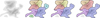 |
Fig. A.1 Illustration of structure identification and merging by HOP on a hypothetical density field. First a collection of peak patches around local maxima is identified. Then, the green structure is rejected because its peak density is not high enough. The cyan structure is merged into the blue one for the same reason. Next, the yellow structure is merged into the red one because the saddle density between the structures is larger than the saddle threshold, indicating that they are connected structures. |
Finally, we discard structures which consist of fewer than the minimum required number of cells. By using this criterion we can select structures that are sufficiently resolved.
The full process is illustrated in Figure A.1.
Appendix A.3 Calculating structure properties
Once we have identified which cells/particles belong to which structure, we calculate the structure properties. Users of our wrapper can easily select what type of properties they want to calculate. One can also easily extend the code to add additional properties of interest. Here we list some elemental ones that are studied in this work.
Appendix A.3.1 Position, mass, density and magnetic field
The total mass M is given by the sum of the masses of each particle or grid cell:
![Mathematical equation: $\[M=\sum_i m_i=\sum_i \rho_i V_i,\]$](/articles/aa/full_html/2024/06/aa48983-23/aa48983-23-eq6.png) (A.1)
(A.1)
where ρi is the density and Vi is the volume of the cell i. The average density is defined as
![Mathematical equation: $\[\rho=\frac{\sum_i m_i}{\sum_i V_i}.\]$](/articles/aa/full_html/2024/06/aa48983-23/aa48983-23-eq7.png) (A.2)
(A.2)
We also determine the maximum density inside the structure and the corresponding peak coordinates. The centre-of-mass coordinates are given by
![Mathematical equation: $\[x=\sum_i m_i x_{o, i} / M,\]$](/articles/aa/full_html/2024/06/aa48983-23/aa48983-23-eq8.png) (A.3)
(A.3)
where we take into account periodic boundaries by first re-centring around the peak location (and assuming the structure is significantly smaller than the box size of the simulation).
Appendix A.3.2 Size and shape
Once we know the centre of mass, we construct the inertia matrix using the centre-of-mass coordinates
![Mathematical equation: $\[I=\left[\begin{array}{ccc}\sum_i m_i\left(y_i^2+z_i^2\right) & -\sum_i m_i x_i y_i & -\sum_i m_i x_i z_i \\-\sum_i m_i x_i y_i & \sum_i m_i\left(x_i^2+z_i^2\right) & -\sum_i m_i y_i z_i \\-\sum_i m_i x_i z_i & -\sum_i m_i y_i z_i & \sum_i m_i\left(x_i^2+y_i^2\right)\end{array}\right],\]$](/articles/aa/full_html/2024/06/aa48983-23/aa48983-23-eq9.png) (A.4)
(A.4)
and find its eigenvalues λ1 ≤ λ2 ≤ λ3 through diagonalisation. We approximate the shape of the clouds by considering the ellipsoid with an uniform density that has the same inertia matrix eigenvalues. The half-axes a ≤ b ≤ c of this ellipsoid are given by
![Mathematical equation: $\[\begin{aligned}& a=\sqrt{\frac{5}{2 M}\left(\lambda_1+\lambda_2-\lambda_3\right)} \\& b=\sqrt{\frac{5}{2 M}\left(\lambda_1+\lambda_3-\lambda_2\right)} \\& c=\sqrt{\frac{5}{2 M}\left(\lambda_2+\lambda_3-\lambda_1\right).}\end{aligned}\]$](/articles/aa/full_html/2024/06/aa48983-23/aa48983-23-eq10.png) (A.5)
(A.5)
We tested visually that the corresponding ellipsoid matches well with the extent of the clouds. While this gives good results, it is worth recalling that clouds have a much more complex shape compared to a simple ellipsoid. We define the average size as the geometric mean of the three half-axes multiplied by 2,
![Mathematical equation: $\[L=2(a b c)^{1 / 3}.\]$](/articles/aa/full_html/2024/06/aa48983-23/aa48983-23-eq11.png) (A.6)
(A.6)
It is important to keep in mind that this definition corresponds to a diameter, rather than a radius.
Appendix A.3.3 Kinematic quantities
The centre-of-mass velocity (a.k.a. the bulk velocity) is simply the mass-weighted average velocity of the cells in the structure:
![Mathematical equation: $\[\bar{\boldsymbol{v}}=\frac{\sum_i m_i \boldsymbol{v}_i}{M}.\]$](/articles/aa/full_html/2024/06/aa48983-23/aa48983-23-eq12.png) (A.7)
(A.7)
The velocity dispersion is obtained using
![Mathematical equation: $\[\sigma=\sqrt{\frac{\sum_i m_i\left|\boldsymbol{v}_i-\bar{\boldsymbol{v}}\right|^2}{M}}.\]$](/articles/aa/full_html/2024/06/aa48983-23/aa48983-23-eq13.png) (A.8)
(A.8)
Appendix A.4 Choosing merge parameters
To determine suitable merge parameters, we first investigate the effect of each individual criterion on the extraction results. More specifically, we look at their influence on the cloud mass spectrum. Figure A.2 shows the results of our tests on LS-weak-driving, a stratified box simulation run with RAMSES. Requiring a minimum number of cells for a structure means we only select the larger objects, as seen in the top panel. As long as we are not too demanding, we recover the same highmass tail. The middle panel shows that peak merging on its own has a minor effect. It merges small structures with low peak-to-background ratios into larger structures, producing a spectrum which is somewhat more top heavy. Finally, the saddle merging has the largest effect on the high-mass slope, as seen in the bottom panel. Setting the ratio to 1 means merging everything that touches. Almost all of the small and intermediate mass structures have been merged into a handful of massive cloud complexes. Disabling saddle merging altogether (that is to say choosing a very large value) results in a sharp cut-off which is basically determined by the resolution. Adding an appropriate saddle merging criterion with respect to the density threshold allows one to recover large structures while keeping a significant population of lower mass objects.
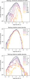 |
Fig. A.2 Effect of the merge parameters on the mass spectrum of the extracted clouds in LS-weak-driving. Top: Changing min_cells while disabling peak and saddle merging. Middle: Varying the ratio rho_peak/rho_thresh, while keeping min_cells=10 and disabling saddle merging. Bottom: Varying the ratio rho_saddle/rho_thresh while keeping min_cells=10 and disabling peak merging. |
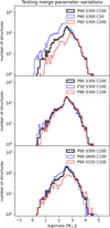 |
Fig. A.3 Effect on the mass spectrum of clouds in LS-weak-driving when varying the merge parameters around the chosen values: min_cells (C) = 100, rho_peak (P) = 2 x rho_thresh, rho_saddle (S) = 10 x rho_thresh. |
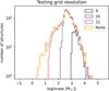 |
Fig. A.4 Study of the influence of resolution on the structure mass spectrum for LS-weak-driving. We limit the loading of the AMR tree to a certain refinement level, as indicated in the legend. Increasing the refinement by one level means the smallest spatial scale resolved becomes a factor two smaller and the volume of a cell is a factor 8 smaller. |
Now that we understand the impact of the merge parameters, we can make an educated choice. We want to obtain a catalogue of structures that are resolved, to avoid having to calculate the properties of unresolved structures close to the resolution limit. We therefore choose min_cells = 100, which accurately recovers the high-mass slope while neglecting a large amount of unresolved objects. Since the peak density criterion plays only a minor role, we can apply any desired signal-to-noise ratio. As a default value, we set rho_peak to be twice rho_thresh. The saddle threshold is the most difficult parameter to choose, and one might want to vary it depending on the application. Our tests show that a value of ten times rho_thresh gives good results. This selects structures in a specified density range and allows for the comparison of simulations with different resolutions, provided the saddle density is resolved in the lowest resolution run. Figure A.3 verifies the mass distribution does not change dramatically when slightly varying the chosen merge parameters.
Appendix A.5 Testing resolution
In Figure A.4 we demonstrate that the high-mass part of the cloud mass spectrum does not depend on the resolution. The cutoff at low masses does depend on resolution, especially since the minimum requested number of cells is kept the same.
Appendix A.6 Testing low density cutoff
In Figure A.5 we demonstrate that it is possible to recover the same cloud mass spectrum when neglecting low density parts of the simulation in the group finding phase of HOP. This is particularly interesting for simulations which contain many particles or cells and are thus memory heavy.
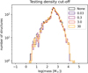 |
Fig. A.5 Study where we limited the input for HOP. to cells above a certain density threshold relative to the extraction threshold. We provide the resulting mass spectrum for LS-weak-driving. |
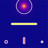 |
Fig. A.6 HOP. detection of simple structures in a synthetic volume. Various spherical or filamentary shapes were correctly detected by HOP. |
Appendix A.7 Tests on idealised structures
To test how good HOP. is at identifying structures and recovering shape information, we run the extraction algorithm on a synthetic volume populated by simple structures (spheres and filaments). HOP. was able to correctly identify all structures and recover the shape parameters (see Section 3.3). This is illustrated by Fig. A.6.
Appendix B Parameters of the galactic simulations
Table B.1 summarises the initial conditions used for the Ramses-F20 and the M51 simulations.
Initial conditions for the full galaxy simulations, with Npart being the resolution in number of particles, Hi the scale height, σi the initial velocity dispersion at a scale of 0.1Hi (when relevant), Ti the initial temperature, and Qmin the minimal value for the Toomre parameter. The gas particles are then used to generate the initial gas density, and the other are used directly.
Appendix C Fit of the mass spectrum
We fitted the mass spectrum in the appropriate range for each individual simulation.
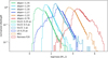 |
Fig. C.1 Fits of the individual cloud mass spectra |
Appendix D Variations with galactic radius
As mentioned in Section 3.1.4 and shown in Figure 5, we did not find a difference in the mass spectrum for the inner versus outer galaxy in our two galaxy simulations, with a boundary between inner and outer zone set at 7 kpc. However, Tress et al. (2021) did find that the masses of clouds in the very centre of the simulated M51 galaxy are typically larger. In Figure D.1 we compare the cumulative distribution for clouds in the inner 1 kpc of our galaxies versus that of clouds located in the remainder of the galaxy. For the cloud mass (top panel) in M51, we recover the qualitative result of Tress et al. (2021). Clouds also have higher velocity dispersions, as can be seen in the bottom panel. The Ramses-F20 galaxy on the other hand, has slightly less massive clouds in the centre and the distribution of velocity dispersions is very similar in both sub-regions. We caution that the statistics in the central region of both galaxies are rather poor.
The weight of the stellar and dark matter component is higher in the centre than in the outskirts. We would expect this to influence the mean statistical properties of the clouds. A more efficient channelling of the gas along the deeper galactic potential in the centre could lead to more massive structures. However this effect is modulated by other aspects, such as higher turbulence and shear which can easily disrupt large clouds. The gas fraction Mgas/(Mgas + Mstars) of the M51 simulation is overall lower than that of Ramses-F20 (see Table B.1). As a consequence, the impact of the weight of the non-gaseous components is higher in M51. This could provide a possible explanation for the different behaviour of the mass spectrum in both galaxies.
Another key difference between the two galaxies is their morphology. In particular, M51 has a central bar while Ramses-F20 does not (see Figure 1). Observations have shown that gas in the centre of barred galaxies has an increased velocity disperion (Sun et al. 2020). We indeed recover this behaviour in the bottom left panel of Figure D.1.
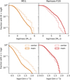 |
Fig. D.1 Comparison between key cloud properties in the centre of the galaxies versus those in the main body. The threshold between the two regions is taken at a galactic radius of 1 kpc. We show the cumulative distribution of cloud mass (top) and cloud velocity dispersion (bottom). |
References
- Audit, E., & Hennebelle, P. 2005, A&A, 433, 1 [CrossRef] [EDP Sciences] [Google Scholar]
- Bahcall, J. N., & Soneira, R. M. 1980, ApJS, 44, 73 [NASA ADS] [CrossRef] [Google Scholar]
- Bakes, E. L. O., & Tielens, A. G. G. M. 1994, ApJ, 427, 822 [NASA ADS] [CrossRef] [Google Scholar]
- Ballesteros-Paredes, J. 2006, MNRAS, 372, 443 [NASA ADS] [CrossRef] [Google Scholar]
- Ballesteros-Paredes, J., & Mac Low, M.-M. 2002, ApJ, 570, 734 [Google Scholar]
- Ballesteros-Paredes, J., Hartmann, L., & Vázquez-Semadeni, E. 1999, ApJ, 527, 285 [NASA ADS] [CrossRef] [Google Scholar]
- Ballesteros-Paredes, J., Hartmann, L. W., Vázquez-Semadeni, E., Heitsch, F., & Zamora-Avilés, M. A. 2011, MNRAS, 411, 65 [NASA ADS] [CrossRef] [Google Scholar]
- Ballesteros-Paredes, J., D’Alessio, P., & Hartmann, L. 2012, MNRAS, 427, 2562 [Google Scholar]
- Ballesteros-Paredes, J., Román-Zúñiga, C., Salomé, Q., Zamora-Avilés, M., & Jiménez-Donaire, M. J. 2019, MNRAS, 490, 2648 [Google Scholar]
- Bate, M. R., Bonnell, I. A., & Bromm, V. 2003, MNRAS, 339, 577 [NASA ADS] [CrossRef] [Google Scholar]
- Beaumont, C. N., Goodman, A. A., Alves, J. F., et al. 2012, MNRAS, 423, 2579 [NASA ADS] [CrossRef] [Google Scholar]
- Benedettini, M., Molinari, S., Baldeschi, A., et al. 2020, A&A, 633, A147 [NASA ADS] [CrossRef] [EDP Sciences] [Google Scholar]
- Benedettini, M., Traficante, A., Olmi, L., et al. 2021, A&A, 654, A144 [NASA ADS] [CrossRef] [EDP Sciences] [Google Scholar]
- Bergin, E. A., Hartmann, L. W., Raymond, J. C., & Ballesteros-Paredes, J. 2004, ApJ, 612, 921 [NASA ADS] [CrossRef] [Google Scholar]
- Bertoldi, F., & McKee, C. F. 1992, ApJ, 395, 140 [NASA ADS] [CrossRef] [Google Scholar]
- Bleuler, A., & Teyssier, R. 2014, MNRAS, 445, 4015 [Google Scholar]
- Blitz, L. 1993, in Protostars and Planets III, eds. E. H. Levy, & J. I. Lunine, 125 [Google Scholar]
- Bolatto, A. D., Leroy, A. K., Rosolowsky, E., Walter, F., & Blitz, L. 2008, ApJ, 686, 948 [NASA ADS] [CrossRef] [Google Scholar]
- Bouchut, F., Klingenberg, C., & Waagan, K. 2007, Numer. Math., 108, 7 [Google Scholar]
- Bouchut, F., Klingenberg, C., & Waagan, K. 2010, Numer. Math., 115, 647 [Google Scholar]
- Brucy, N. 2022, PhD thesis, CEA Saclay, Service d’Astrophysique, France [Google Scholar]
- Brucy, N., Hennebelle, P., Bournaud, F., & Colling, C. 2020, ApJ, 896, L34 [NASA ADS] [CrossRef] [Google Scholar]
- Brucy, N., Hennebelle, P., Colman, T., & Iteanu, S. 2023, A&A, 675, A144 [NASA ADS] [CrossRef] [EDP Sciences] [Google Scholar]
- Cahlon, S., Zucker, C., Goodman, A., Lada, C., & Alves, J. 2024, ApJ, 961, 153 [NASA ADS] [CrossRef] [Google Scholar]
- Chabrier, G. 2003, PASP, 115, 763 [Google Scholar]
- Chen, B. Q., Huang, Y., Yuan, H. B., et al. 2019, MNRAS, 483, 4277 [Google Scholar]
- Chen, B. Q., Li, G. X., Yuan, H. B., et al. 2020, MNRAS, 493, 351 [NASA ADS] [CrossRef] [Google Scholar]
- Chevance, M., Krumholz, M. R., McLeod, A. F., et al. 2023, in ASP Conf. Ser., 534, Protostars and Planets VII, eds. S. Inutsuka, Y. Aikawa, T. Muto, K. Tomida, & M. Tamura, 1 [Google Scholar]
- Clarke, C., & Oey, M. S. 2002, MNRAS, 337, 1299 [NASA ADS] [CrossRef] [Google Scholar]
- Clark, P. C., Glover, S. C. O., & Klessen, R. S. 2012, MNRAS, 420, 745 [NASA ADS] [CrossRef] [Google Scholar]
- Clark, P. C., Glover, S. C. O., Ragan, S. E., & Duarte-Cabral, A. 2019, MNRAS, 486, 4622 [Google Scholar]
- Colling, C., Hennebelle, P., Geen, S., Iffrig, O., & Bournaud, F. 2018, A&A, 620, A21 [NASA ADS] [CrossRef] [EDP Sciences] [Google Scholar]
- Colman, T., Robitaille, J.-F., Hennebelle, P., et al. 2022, MNRAS, 514, 3670 [NASA ADS] [CrossRef] [Google Scholar]
- Colombo, D., Hughes, A., Schinnerer, E., et al. 2014, ApJ, 784, 3 [NASA ADS] [CrossRef] [Google Scholar]
- Colombo, D., Rosolowsky, E., Ginsburg, A., Duarte-Cabral, A., & Hughes, A. 2015, MNRAS, 454, 2067 [NASA ADS] [CrossRef] [Google Scholar]
- Colombo, D., Rosolowsky, E., Duarte-Cabral, A., et al. 2019, MNRAS, 483, 4291 [NASA ADS] [CrossRef] [Google Scholar]
- Crutcher, R. M. 2012, ARA&A, 50, 29 [Google Scholar]
- Dame, T. M., Ungerechts, H., Cohen, R. S., et al. 1987, ApJ, 322, 706 [NASA ADS] [CrossRef] [Google Scholar]
- Dame, T. M., Hartmann, D., & Thaddeus, P. 2001, ApJ, 547, 792 [Google Scholar]
- de Avillez, M. A. 2000, MNRAS, 315, 479 [NASA ADS] [CrossRef] [Google Scholar]
- de Avillez, M. A., & Breitschwerdt, D. 2005, A&A, 436, 585 [NASA ADS] [CrossRef] [EDP Sciences] [Google Scholar]
- Dharmawardena, T. E., Bailer-Jones, C. A. L., Fouesneau, M., et al. 2023, MNRAS, 519, 228 [Google Scholar]
- Donovan Meyer, J., Koda, J., Momose, R., et al. 2013, ApJ, 772, 107 [NASA ADS] [CrossRef] [Google Scholar]
- Draine, B. T. 1978, ApJS, 36, 595 [Google Scholar]
- Draine, B. T. 2011, Physics of the Interstellar and Intergalactic Medium (Princeton University Press) [CrossRef] [Google Scholar]
- Duarte-Cabral, A., Colombo, D., Urquhart, J. S., et al. 2021, MNRAS 500, 3027 [Google Scholar]
- Dubey, A., Fisher, R., Graziani, C., et al. 2008, in ASP Conf. Ser., 385, Numerical Modeling of Space Plasma Flows, eds. N. V. Pogorelov, E. Audit, & G. P. Zank, 145 [Google Scholar]
- Ebagezio, S., Seifried, D., Walch, S., et al. 2023, MNRAS, 525, 5631 [NASA ADS] [CrossRef] [Google Scholar]
- Eisenstein, D. J., & Hut, P. 1998, ApJ, 498, 137 [NASA ADS] [CrossRef] [Google Scholar]
- Elmegreen, B. G., & Falgarone, E. 1996, ApJ, 471, 816 [NASA ADS] [CrossRef] [Google Scholar]
- Elmegreen, B. G., & Elmegreen, D. M. 2001, ApJ, 121, 1507 [CrossRef] [Google Scholar]
- Elmegreen, B. G., & Scalo, J. 2004, ARA&A, 42, 211 [Google Scholar]
- Falgarone, E., Phillips, T. G., & Walker, C. K. 1991, ApJ, 378, 186 [NASA ADS] [CrossRef] [Google Scholar]
- Federrath, C., & Klessen, R. S. 2012, ApJ, 761, 156 [Google Scholar]
- Fromang, S., Hennebelle, P., & Teyssier, R. 2006, A&A, 457, 371 [NASA ADS] [CrossRef] [EDP Sciences] [Google Scholar]
- Fryxell, B., Olson, K., Ricker, P., et al. 2000, ApJS, 131, 273 [Google Scholar]
- Fukui, Y., Kawamura, A., Minamidani, T., et al. 2008, ApJS, 178, 56 [Google Scholar]
- Geen, S., Hennebelle, P., Tremblin, P., & Rosdahl, J. 2016, MNRAS, 463, 3129 [CrossRef] [Google Scholar]
- Gent, F. A., Shukurov, A., Fletcher, A., Sarson, G. R., & Mantere, M. J. 2013, MNRAS, 432, 1396 [NASA ADS] [CrossRef] [Google Scholar]
- Girichidis, P. 2021, MNRAS, 507, 5641 [NASA ADS] [CrossRef] [Google Scholar]
- Girichidis, P., Walch, S., Naab, T., et al. 2016, MNRAS, 456, 3432 [NASA ADS] [CrossRef] [Google Scholar]
- Girichidis, P., Seifried, D., Naab, T., et al. 2018, MNRAS, 480, 3511 [NASA ADS] [CrossRef] [Google Scholar]
- Glover, S. C. O., & Clark, P. C. 2012a, MNRAS, 421, 116 [NASA ADS] [Google Scholar]
- Glover, S. C. O., & Clark, P. C. 2012b, MNRAS, 421, 9 [NASA ADS] [Google Scholar]
- Glover, S. C. O., & Mac Low, M.-M. 2007a, ApJS, 169, 239 [NASA ADS] [CrossRef] [Google Scholar]
- Glover, S. C. O., & Mac Low, M.-M. 2007b, ApJ, 659, 1317 [NASA ADS] [CrossRef] [Google Scholar]
- Glover, S. C. O., Federrath, C., Mac Low, M.-M., & Klessen, R. S. 2010, MNRAS, 404, 2 [NASA ADS] [Google Scholar]
- Gnat, O., & Ferland, G. J. 2012, ApJS, 199, 20 [NASA ADS] [CrossRef] [Google Scholar]
- Goldsmith, P. F. 2001, ApJ, 557, 736 [Google Scholar]
- Goldsmith, P. F., & Langer, W. D. 1978, ApJ, 222, 881 [Google Scholar]
- Gratier, P., Braine, J., Rodriguez-Fernandez, N. J., et al. 2012, A&A, 542, A108 [NASA ADS] [CrossRef] [EDP Sciences] [Google Scholar]
- Habing, H. J. 1968, Bull. Astron. Inst. Netherlands, 19, 421 [Google Scholar]
- Heiles, C. 1987, ApJ, 315, 555 [NASA ADS] [CrossRef] [Google Scholar]
- Hennebelle, P., & Chabrier, G. 2008, ApJ, 684, 395 [Google Scholar]
- Hennebelle, P., & Chabrier, G. 2011, ApJ, 743, L29 [Google Scholar]
- Hennebelle, P., & Falgarone, E. 2012, A&A Rev., 20, 55 [NASA ADS] [CrossRef] [Google Scholar]
- Hernquist, L. 1990, ApJ, 356, 359 [Google Scholar]
- Heyer, M. H., & Brunt, C. M. 2004, ApJ, 615, L45 [NASA ADS] [CrossRef] [Google Scholar]
- Heyer, M., & Dame, T. M. 2015, ARA&A, 53, 583 [Google Scholar]
- Heyer, M. H., Carpenter, J. M., & Snell, R. L. 2001, ApJ, 551, 852 [NASA ADS] [CrossRef] [Google Scholar]
- Heyer, M., Krawczyk, C., Duval, J., & Jackson, J. M. 2009, ApJ, 699, 1092 [Google Scholar]
- Hill, A. S., Joung, M. R., Mac Low, M.-M., et al. 2012, ApJ, 750, 104 [NASA ADS] [CrossRef] [Google Scholar]
- Hollenbach, D., & McKee, C. F. 1989, ApJ, 342, 306 [Google Scholar]
- Hopkins, P. F. 2012, MNRAS, 423, 2016 [NASA ADS] [CrossRef] [Google Scholar]
- Iffrig, O., & Hennebelle, P. 2017, A&A, 604, A70 [NASA ADS] [CrossRef] [EDP Sciences] [Google Scholar]
- Jeffreson, S. M. R., Kruijssen, J. M. D., Keller, B. W., Chevance, M., & Glover, S. C. O. 2020, MNRAS, 498, 385 [Google Scholar]
- Joung, M. K. R., & Mac Low, M.-M. 2006, ApJ, 653, 1266 [NASA ADS] [CrossRef] [Google Scholar]
- Joung, M. R., Mac Low, M.-M., & Bryan, G. L. 2009, ApJ, 704, 137 [NASA ADS] [CrossRef] [Google Scholar]
- Kauffmann, J., Pillai, T., & Goldsmith, P. F. 2013, ApJ, 779, 185 [NASA ADS] [CrossRef] [Google Scholar]
- Kennicutt, Jr., R. C. 1998, ApJ, 498, 541 [Google Scholar]
- Kennicutt, Robert, C., J., Edgar, B. K., & Hodge, P. W. 1989, ApJ, 337, 761 [NASA ADS] [CrossRef] [Google Scholar]
- Kim, W.-T., & Ostriker, E. C. 2007, ApJ, 660, 1232 [NASA ADS] [CrossRef] [Google Scholar]
- Kim, C.-G., & Ostriker, E. C. 2017, ApJ, 846, 133 [NASA ADS] [CrossRef] [Google Scholar]
- Klessen, R. S., & Burkert, A. 2000, ApJS, 128, 287 [NASA ADS] [CrossRef] [Google Scholar]
- Klessen, R. S., & Glover, S. C. O. 2016, Star Formation in Galaxy Evolution: Connecting Numerical Models to Reality, Saas-Fee Advanced Course (Springer-Verlag Berlin Heidelberg) 85 [NASA ADS] [CrossRef] [Google Scholar]
- Kretschmer, M., & Teyssier, R. 2020, MNRAS, 492, 1385 [Google Scholar]
- Kritsuk, A. G., Norman, M. L., Padoan, P., & Wagner, R. 2007, ApJ, 665, 416 [NASA ADS] [CrossRef] [Google Scholar]
- Krumholz, M. R., & McKee, C. F. 2005, ApJ, 630, 250 [Google Scholar]
- Krumholz, M. R., McKee, C. F., & Klein, R. I. 2005, Nature, 438, 332 [NASA ADS] [CrossRef] [Google Scholar]
- Kuijken, K., & Gilmore, G. 1989, MNRAS, 239, 605 [Google Scholar]
- Kuznetsova, A., Hartmann, L., Heitsch, F., & Ballesteros-Paredes, J. 2018, ApJ, 868, 50 [NASA ADS] [CrossRef] [Google Scholar]
- Lada, C. J., & Dame, T. M. 2020, ApJ, 898, 3 [NASA ADS] [CrossRef] [Google Scholar]
- Larson, R. B. 1981, MNRAS, 194, 809 [Google Scholar]
- Leike, R. H., Glatzle, M., & Enßlin, T. A. 2020, A&A, 639, A138 [NASA ADS] [CrossRef] [EDP Sciences] [Google Scholar]
- Lombardi, M., Alves, J., & Lada, C. J. 2010, A&A, 519, L7 [NASA ADS] [CrossRef] [EDP Sciences] [Google Scholar]
- Ma, Y., Wang, H., Zhang, M., et al. 2022, ApJS, 262, 16 [NASA ADS] [CrossRef] [Google Scholar]
- Mac Low, M.-M., & Klessen, R. S. 2004, Rev. Mod. Phys., 76, 125 [Google Scholar]
- Martizzi, D., Fielding, D., Faucher-Giguère, C.-A., & Quataert, E. 2016, MNRAS, 459, 2311 [NASA ADS] [CrossRef] [Google Scholar]
- Mathis, J. S., Mezger, P. G., & Panagia, N. 1983, A&A, 128, 212 [NASA ADS] [Google Scholar]
- McKee, C. F., & Ostriker, E. C. 2007, ARA&A, 45, 565 [Google Scholar]
- McKee, C. F., & Williams, J. P. 1997, ApJ, 476, 144 [CrossRef] [Google Scholar]
- Micic, M., Glover, S. C. O., Federrath, C., & Klessen, R. S. 2012, MNRAS, 421, 2531 [NASA ADS] [CrossRef] [Google Scholar]
- Miville-Deschênes, M.-A., Murray, N., & Lee, E. J. 2017, ApJ, 834, 57 [Google Scholar]
- Mouschovias, T. C., & Spitzer, Jr., L. 1976, ApJ, 210, 326 [NASA ADS] [CrossRef] [Google Scholar]
- Mouschovias, T. C., & Ciolek, G. E. 1999, in NATO Advanced Science Institutes (ASI) Series C, 540, 305 [Google Scholar]
- Navarro, J. F., Frenk, C. S., & White, S. D. M. 1996, ApJ, 462, 563 [Google Scholar]
- Nelson, R. P., & Langer, W. D. 1997, ApJ, 482, 796 [NASA ADS] [CrossRef] [Google Scholar]
- Oka, T., Hasegawa, T., Sato, F., et al. 2001, ApJ, 562, 348 [Google Scholar]
- Ossenkopf, V., & Henning, T. 1994, A&A, 291, 943 [NASA ADS] [Google Scholar]
- Ostriker, E. C., Stone, J. M., & Gammie, C. F. 2001, ApJ, 546, 980 [Google Scholar]
- Padoan, P., Nordlund, Å., Kritsuk, A. G., Norman, M. L., & Li, P. S. 2007, ApJ, 661, 972 [NASA ADS] [CrossRef] [Google Scholar]
- Ramírez-Galeano, L., Ballesteros-Paredes, J., Smith, R. J., Camacho, V., & Zamora-Avilés, M. 2022, MNRAS, 515, 2822 [CrossRef] [Google Scholar]
- Reid, M. J. 2022, AJ, 164, 133 [NASA ADS] [CrossRef] [Google Scholar]
- Rice, T. S., Goodman, A. A., Bergin, E. A., Beaumont, C., & Dame, T. M. 2016, ApJ, 822, 52 [Google Scholar]
- Roman-Duval, J., Jackson, J. M., Heyer, M., Rathborne, J., & Simon, R. 2010, ApJ, 723, 492 [NASA ADS] [CrossRef] [Google Scholar]
- Rosdahl, J., Blaizot, J., Aubert, D., Stranex, T., & Teyssier, R. 2013, MNRAS, 436, 2188 [Google Scholar]
- Rosolowsky, E. 2005, PASP, 117, 1403 [NASA ADS] [CrossRef] [Google Scholar]
- Rosolowsky, E. W., Pineda, J. E., Kauffmann, J., & Goodman, A. A. 2008, ApJ, 679, 1338 [Google Scholar]
- Rosolowsky, E., Hughes, A., Leroy, A. K., et al. 2021, MNRAS, 502, 1218 [NASA ADS] [CrossRef] [Google Scholar]
- Salpeter, E. E. 1955, ApJ, 121, 161 [Google Scholar]
- Sanders, D. B., Scoville, N. Z., & Solomon, P. M. 1985, ApJ, 289, 373 [NASA ADS] [CrossRef] [Google Scholar]
- Schneider, N., Bontemps, S., Simon, R., et al. 2011, A&A, 529, A1 [NASA ADS] [CrossRef] [EDP Sciences] [Google Scholar]
- Schuller, F., Csengeri, T., Urquhart, J. S., et al. 2017, A&A, 601, A124 [NASA ADS] [CrossRef] [EDP Sciences] [Google Scholar]
- Scoville, N. Z., Yun, M. S., Clemens, D. P., Sanders, D. B., & Waller, W. H. 1987, ApJS, 63, 821 [NASA ADS] [CrossRef] [Google Scholar]
- Seifried, D., Walch, S., Girichidis, P., et al. 2017, MNRAS, 472, 4797 [NASA ADS] [CrossRef] [Google Scholar]
- Shetty, R., Collins, D. C., Kauffmann, J., et al. 2010, ApJ, 712, 1049 [NASA ADS] [CrossRef] [Google Scholar]
- Shu, F. H., Adams, F. C., & Lizano, S. 1987, ARA&A, 25, 23 [Google Scholar]
- Simpson, C. M., Pakmor, R., Marinacci, F., et al. 2016, ApJ, 827, L29 [NASA ADS] [CrossRef] [Google Scholar]
- Singh, A., Matzner, C. D., Friesen, R. K., et al. 2021, ApJ, 922, 87 [CrossRef] [Google Scholar]
- Snow, T. P., & McCall, B. J. 2006, ARA&A, 44, 367 [NASA ADS] [CrossRef] [Google Scholar]
- Solomon, P. M., Rivolo, A. R., Barrett, J., & Yahil, A. 1987, ApJ, 319, 730 [Google Scholar]
- Sormani, M. C., Sobacchi, E., Shore, S. N., Treß, R. G., & Klessen, R. S. 2017, MNRAS, 471, 2932 [NASA ADS] [CrossRef] [Google Scholar]
- Spitzer, Jr., L. 1942, ApJ, 95, 329 [NASA ADS] [CrossRef] [Google Scholar]
- Springel, V. 2010, MNRAS, 401, 791 [Google Scholar]
- Stone, J. M., Ostriker, E. C., & Gammie, C. F. 1998, ApJ, 508, L99 [Google Scholar]
- Sun, J., Leroy, A. K., Schinnerer, E., et al. 2020, ApJ, 901, L8 [NASA ADS] [CrossRef] [Google Scholar]
- Szűcs, L., Glover, S. C. O., & Klessen, R. S. 2016, MNRAS, 460, 82 [CrossRef] [Google Scholar]
- Teyssier, R. 2002, A&A, 385, 337 [CrossRef] [EDP Sciences] [Google Scholar]
- Tielens, A. G. G. M. 2010, The Physics and Chemistry of the Interstellar Medium (Cambridge University Press) [Google Scholar]
- Toomre, A. 1964, ApJ, 139, 1217 [Google Scholar]
- Traficante, A., Duarte-Cabral, A., Elia, D., & et al. 2018a, MNRAS, 477, 2220 [NASA ADS] [CrossRef] [Google Scholar]
- Traficante, A., Lee, Y. N., Hennebelle, P., & et al. 2018b, A&A, 619, A7 [NASA ADS] [CrossRef] [EDP Sciences] [Google Scholar]
- Tress, R. G., Smith, R. J., Sormani, M. C., et al. 2020, MNRAS, 492, 2973 [Google Scholar]
- Tress, R. G., Sormani, M. C., Smith, R. J., et al. 2021, MNRAS, 505, 5438 [NASA ADS] [CrossRef] [Google Scholar]
- Urquhart, J. S., König, C., Giannetti, A., & et al. 2018, MNRAS, 473, 1059 [Google Scholar]
- van der Wel, A., Chang, Y.-Y., Bell, E. F., et al. 2014, ApJ, 792, L6 [NASA ADS] [CrossRef] [Google Scholar]
- Vazquez-Semadeni, E. 1994, ApJ, 423, 681 [Google Scholar]
- Vazquez-Semadeni, E., Passot, T., & Pouquet, A. 1995, ApJ, 441, 702 [NASA ADS] [CrossRef] [Google Scholar]
- Vázquez-Semadeni, E., González-Samaniego, A., & Colín, P. 2017, MNRAS, 467, 1313 [NASA ADS] [Google Scholar]
- Vázquez-Semadeni, E., Palau, A., Ballesteros-Paredes, J., Gómez, G. C., & Zamora-Avilés, M. 2019, MNRAS, 490, 3061 [Google Scholar]
- Waagan, K. 2009, J. Computat. Phys., 228, 8609 [NASA ADS] [CrossRef] [Google Scholar]
- Waagan, K., Federrath, C., & Klingenberg, C. 2011, J. Computat. Phys., 230, 3331 [NASA ADS] [CrossRef] [Google Scholar]
- Walch, S. K., Whitworth, A. P., Bisbas, T., Wünsch, R., & Hubber, D. 2012, MNRAS, 427, 625 [NASA ADS] [CrossRef] [Google Scholar]
- Walch, S., Girichidis, P., Naab, T., et al. 2015, MNRAS, 454, 238 [Google Scholar]
- Whitworth, D. J., Smith, R. J., Klessen, R. S., et al. 2023, MNRAS, 520, 89 [NASA ADS] [CrossRef] [Google Scholar]
- Williams, J. P., & McKee, C. F. 1997, ApJ, 476, 166 [NASA ADS] [CrossRef] [Google Scholar]
- Wolfire, M. G., Hollenbach, D., McKee, C. F., Tielens, A. G. G. M., & Bakes, E. L. O. 1995, ApJ, 443, 152 [Google Scholar]
- Wolfire, M. G., McKee, C. F., Hollenbach, D., & Tielens, A. G. G. M. 2003, ApJ, 587, 278 [Google Scholar]
- Wong, T., Hughes, A., Ott, J., et al. 2011, ApJS, 197, 16 [NASA ADS] [CrossRef] [Google Scholar]
- Wünsch, R., Walch, S., Dinnbier, F., & Whitworth, A. 2018, MNRAS, 475, 3393 [CrossRef] [Google Scholar]
The actual minimal size depends of the shape, but we note that ![Mathematical equation: $\[\sqrt[3]{100} \approx 4.64\]$](/articles/aa/full_html/2024/06/aa48983-23/aa48983-23-eq14.png) .
.
This information is in principle retrievable from clouds detected in 3D dust. However, so far no study has reported sizes along three orthogonal axes.
The question of whether the conventional definition of αvir is an adequate diagnostic of whether or not clouds are gravitationally bound is an interesting one (see e.g. Ramírez-Galeano et al. 2022), but is out of the scope of this study.
For regular grids we take the cell centre. For moving mesh codes, one can either pick the centre of mass in a cell or the location of the mesh generating point. In this work we opted for the latter. We note that in AREPO a mesh generating point is steered towards the centre of mass of the cell, so both are equivalent to first order.
All Tables
Compilation of observational studies, with summary of their underlying data used to produce the molecular cloud catalogue, and their reported mass-size relation.
Number of cells and fractions of cells on each refinement level for the stratified box simulations.
Initial conditions for the full galaxy simulations, with Npart being the resolution in number of particles, Hi the scale height, σi the initial velocity dispersion at a scale of 0.1Hi (when relevant), Ti the initial temperature, and Qmin the minimal value for the Toomre parameter. The gas particles are then used to generate the initial gas density, and the other are used directly.
All Figures
|
Fig. 1 Column density map for a single snapshot from each of the four listed groups of simulations. The panels show SILCC-0.5pc-3μG (a), LS-weak-driving (b), M51 (c), Ramses-F20 (d). Details of these simulations can be found in Table 1. The coloured symbols indicate the locations of the clouds identified by the HOP algorithm, with the colour corresponding to the internal velocity dispersion. |
| In the text | |
|
Fig. 2 Column density maps of selected clouds extracted from the simulations. The different rows show examples from SILCC-0.5-pc (a), LS-no-driving (b), M51 (c), Ramses-F20 (d). Column density is calculated in a box of three times the maximum extent of the object. Labels are added showing the cloud mass and velocity dispersion. The coloured symbol is used to refer to the cloud in the following figures in the paper. |
| In the text | |
|
Fig. 3 3D visualisations of the clouds from Fig. 2b, extracted from the LS stratified box simulations. The density scale is linear. The ellipsoid approximation (in cyan) and its half-axes (in black) are also shown. |
| In the text | |
|
Fig. 4 Comparison of the mass (top) and size (bottom) distribution of clouds in the different simulations, normalised according to the relevant surface area of the simulation. To guide the eye, we add a grey line indicating an appropriate power-law slopes of −1 for the mass spectrum in the top panel and −3 for the size distribution in the bottom panel. The dashed lines correspond to multiples of the spacial resolution in the SILCC and LS simulations. The dotted lines show multiples of the resolution for the Ramses galaxy. |
| In the text | |
|
Fig. 5 Comparison of the mass distribution of clouds in the inner 7 kpc of a galaxy versus those in the outskirts. While Ramses-F20 overall has a shallower mass spectrum than M51 (and the kpc boxes), there is no difference in the measured slope between the inner and the outer galaxy for either simulation. |
| In the text | |
|
Fig. 6 Correlation between cloud size and mass, with the size computed in two different ways. In panel a, the size is defined as the average between the three half-axis of the approximating ellipse, as determined by the structure algorithm. In panel b, the size is computed as the cubic root of the volume. Each dot represents one cloud. The contour lines show a kernel density estimate of the distribution. Starting from the innermost line, approximately 10, 30, 50, and 70% of the distribution lie within the respective contours. The symbols highlight the example clouds from Fig. 2. The grey line in panel a indicates a slope of 3. The solid and dotted line in panel b are iso-density lines for the detection and saddle threshold respectively, as defined in Sec. 2.1 and Appendix A. Their slopes are 3. |
| In the text | |
|
Fig. 7 General shapes of the clouds within the simulations. Panel a: relation between the ratio of the middle half-axis over the largest b/c and the ratio of the smallest half-axis over the largest a/c assuming clouds have a ellipsoidal shape. The characterisation of the shape the one used in van der Wel et al. (2014). The contour lines and symbols are the same as in Fig. 6a. Panel b: marginal distributions of the ratio of the ellipsoidal half-axes of the clouds between the simulations. |
| In the text | |
|
Fig. 8 Sphericity as a function of structure size, computed from the volume (a) or the number of cells (b). The solid line depicts the mean in a logarithmic bin of size, and is computed only if the bin contains at least 100 clouds. Contour lines and symbols are as in Fig. 6a. |
| In the text | |
|
Fig. 9 Cloud velocity dispersion as a function of the size. The dashed line illustrates a scaling of σ with size R0.75 while the curved solid line illustrates the trend of the centroids of each distributions. The contour lines and symbols are the same as in Fig. 6. |
| In the text | |
|
Fig. 10 Comparison of the 3D size-velocity dispersion relation found in the simulation with several cloud catalogues from observations. Coloured contours are as in Fig. 6. Observational data feature only the 1D line-of-sight velocity dispersion, which was here multiplied by |
| In the text | |
|
Fig. 11 Two examples showing the positions of the clouds with their respective density (left), temperature (middle), and velocity environment (right). In both cases the clouds are located at the edge between cold gas and a hot SN-driven bubble. The resulting high velocity dispersion is thus due to SN-driven turbulence that mixes hot gas into the clouds rather than by gravitational collapse. |
| In the text | |
|
Fig. 12 Scatter plot of the velocity distribution as a function of cloud mass for simulation SILCC-0.5pc. Left: colours indicate the mass-weighted temperature in a sphere around the centre of the HOP cloud with a radius corresponding to twice the average size of the HOP cloud. Right: colours indicate the molecular fraction in the surrounding sphere. |
| In the text | |
|
Fig. 13 Virial parameter as a function of cloud mass for all simulations. Coloured contour lines are the same as in Fig. 6. Over-plotted are the slope of the scaling (thick grey line), as well as the observational data compiled for the PPVII review (Chevance et al. 2023). |
| In the text | |
|
Fig. 14 Distribution of cloud-averaged temperatures. |
| In the text | |
|
Fig. 15 Comparison of the cloud mass spectrum in two RAMSES test simulations with a similar setup to simulation LS using different refinement strategies. |
| In the text | |
|
Fig. 16 Mass-size relation for the LS stratified boxes and M51 galaxy when using our default HOP parameters versus FOF-like merge criteria. Coloured contour lines are the same as in Fig. 6a. |
| In the text | |
|
Fig. A.1 Illustration of structure identification and merging by HOP on a hypothetical density field. First a collection of peak patches around local maxima is identified. Then, the green structure is rejected because its peak density is not high enough. The cyan structure is merged into the blue one for the same reason. Next, the yellow structure is merged into the red one because the saddle density between the structures is larger than the saddle threshold, indicating that they are connected structures. |
| In the text | |
|
Fig. A.2 Effect of the merge parameters on the mass spectrum of the extracted clouds in LS-weak-driving. Top: Changing min_cells while disabling peak and saddle merging. Middle: Varying the ratio rho_peak/rho_thresh, while keeping min_cells=10 and disabling saddle merging. Bottom: Varying the ratio rho_saddle/rho_thresh while keeping min_cells=10 and disabling peak merging. |
| In the text | |
|
Fig. A.3 Effect on the mass spectrum of clouds in LS-weak-driving when varying the merge parameters around the chosen values: min_cells (C) = 100, rho_peak (P) = 2 x rho_thresh, rho_saddle (S) = 10 x rho_thresh. |
| In the text | |
|
Fig. A.4 Study of the influence of resolution on the structure mass spectrum for LS-weak-driving. We limit the loading of the AMR tree to a certain refinement level, as indicated in the legend. Increasing the refinement by one level means the smallest spatial scale resolved becomes a factor two smaller and the volume of a cell is a factor 8 smaller. |
| In the text | |
|
Fig. A.5 Study where we limited the input for HOP. to cells above a certain density threshold relative to the extraction threshold. We provide the resulting mass spectrum for LS-weak-driving. |
| In the text | |
|
Fig. A.6 HOP. detection of simple structures in a synthetic volume. Various spherical or filamentary shapes were correctly detected by HOP. |
| In the text | |
|
Fig. C.1 Fits of the individual cloud mass spectra |
| In the text | |
|
Fig. D.1 Comparison between key cloud properties in the centre of the galaxies versus those in the main body. The threshold between the two regions is taken at a galactic radius of 1 kpc. We show the cumulative distribution of cloud mass (top) and cloud velocity dispersion (bottom). |
| In the text | |
Current usage metrics show cumulative count of Article Views (full-text article views including HTML views, PDF and ePub downloads, according to the available data) and Abstracts Views on Vision4Press platform.
Data correspond to usage on the plateform after 2015. The current usage metrics is available 48-96 hours after online publication and is updated daily on week days.
Initial download of the metrics may take a while.