| Issue |
A&A
Volume 686, June 2024
|
|
|---|---|---|
| Article Number | A53 | |
| Number of page(s) | 18 | |
| Section | Planets and planetary systems | |
| DOI | https://doi.org/10.1051/0004-6361/202348596 | |
| Published online | 29 May 2024 | |
The interplay between forming planets and photoevaporating discs
II. Wind-driven gas redistribution
1
University Observatory, Faculty of Physics, Ludwig-Maximilians-Universität München,
Scheinerstr. 1,
81679
Munich,
Germany
e-mail: This email address is being protected from spambots. You need JavaScript enabled to view it.
2
Excellence Cluster ORIGINS,
Boltzmannstr. 2,
85748
Garching,
Germany
Received:
13
November
2023
Accepted:
16
February
2024
Abstract
Context. Disc winds and planet–disc interactions are two crucial mechanisms that define the structure, evolution, and dispersal of protoplanetary discs. While winds are capable of removing material from discs, eventually leading to their dispersal, massive planets can shape their disc by creating sub-structures such as gaps and spiral arms.
Aims. We studied the interplay between an X-ray photoevaporative disc wind and the sub-structures generated due to planet–disc interactions to determine how their mutual interactions affect the disc’s and the planet’s evolution.
Methods. We performed 3D hydrodynamic simulations of viscous discs (α = 6.9 × 10⁻⁴) that host a Jupiter-like planet and undergo X-ray photoevaporation. We traced the gas flows within the disc and wind and measured the rate of accretion onto the planet, as well as the gravitational torque that is acting on it.
Results. Our results show that the planetary gap removes the wind’s pressure support, allowing wind material to fall back into the gap. This opens new pathways for material from the inner disc (and part of the outer disc) to be redistributed through the wind towards the gap. Consequently, the gap becomes shallower and the flow of mass across the gap in both directions is significantly increased, as is the planet’s mass-accretion rate (by factors of ≈5 and ≈2, respectively). Moreover, the wind-driven redistribution results in a denser inner disc and a less dense outer disc, which, combined with the recycling of a significant portion of the inner wind, leads to longer lifetimes for the inner disc, contrary to the expectation in a planet-induced photoevaporation scenario that has been proposed in the past.
Key words: hydrodynamics / protoplanetary disks / planet–disk interactions
© The Authors 2024
 Open Access article, published by EDP Sciences, under the terms of the Creative Commons Attribution License (https://creativecommons.org/licenses/by/4.0), which permits unrestricted use, distribution, and reproduction in any medium, provided the original work is properly cited.
This article is published in open access under the Subscribe to Open model. This email address is being protected from spambots. You need JavaScript enabled to view it. to support open access publication.
1 Introduction
The extensive diversity of exoplanets and exoplanetary systems discovered in recent years highlights the importance of understanding the many different processes involved in the formation and evolution of planets in protoplanetary discs. Two of the most important processes that can affect the structure, evolution, and dispersal of protoplanetary discs are planet–disc interactions and disc winds.
Through the gravitational influence on its surrounding material, a newly formed planet that is still embedded in a protoplanetary disc can generate complex sub-structures in the disc that can influence both the planet’s and the disc’s evolution (see e.g. Paardekooper et al. 2023, for a recent review). A planet excites spiral density waves at Lindblad resonances, and if the planet is massive enough, the torque that the spiral waves exert on the disc can become strong enough to overcome the viscous torque, at which point a gap will open in the disc along the planet’s orbit (Goldreich & Tremaine 1979, 1980; Papaloizou & Lin 1984). Numerical simulations show that at the edges of such gaps, the gas follows meridional flows, circulating between the lower and upper layers of the protoplanetary disc (e.g. Morbidelli et al. 2014; Fung & Chiang 2016). The disc, on the other hand, also has a gravitational influence on the planet, and asymmetric sub-structures in the disc can result in a net torque that acts on the planet, changing its angular momentum; this will lead to its migration through the disc, either radially inwards or outwards (e.g. Kley & Nelson 2012, and references therein). Recent observations, for example with the Atacama Large Mil-limeter/submillimeter Array (ALMA), have revealed that most discs are indeed highly sub-structured, including, among other features, gaps, spirals, and meridional flows that may be linked to the presence of planets (see e.g. the review by Pinte et al. 2023). These observations present an excellent testbed for theoretical models of planet–disc interactions. Interpreting them, however, requires a complex understanding of all the different processes at play.
During the last few decades, observational campaigns spanning multiple star-forming regions have shown that most protoplanetary discs have lifetimes of only a few million years (Haisch et al. 2001; Mamajek et al. 2009; Fedele et al. 2010; Ribas et al. 2014). Moreover, the observed disc fractions at different wavelengths suggest that most discs disperse from the inside out (see also Koepferl et al. 2013; Ercolano et al. 2015). While many physical processes have been proposed to drive the dispersal of discs, it is still mostly unconstrained which process is dominant at a given location and time. It is clear that accretion onto the star plays a major role in the disc’s evolution, but the mechanism that is responsible for the necessary transport of angular momentum is still uncertain and could be turbulence driven by various types of instabilities, magnetic winds, or a combination of the two (e.g. Lesur et al. 2023, for a recent review). Very likely, the dominant process varies with the location in the disc and its evolutionary stage. In recent years, magnetically driven disc winds have been shown to be able to drive mass loss and accretion at rates compatible with observations (e.g. Gressel et al. 2015,2020; Bai et al. 2016; Béthune et al. 2017; Wang et al. 2019; Lesur 2021), adding to a growing body of evidence that they play an important role in disc evolution, especially at early stage; later in the disc’s life, thermal winds may become the dominant dispersal mechanism (see also Ercolano & Pascucci 2017; Pascucci et al. 2020,2023). Models of thermal winds, in particular those driven by internal photoevaporation, have been very successful at explaining the lifetimes and fast inside-out dispersal of protoplanetary discs (e.g. Alexander et al. 2006; Gorti & Hollenbach 2009; Owen et al. 2010; Picogna et al. 2019), as well as numerous other observables, including some of the observed spectra of wind-tracing emission lines (Ercolano & Owen 2010, 2016; Weber et al. 2020; Rab et al. 2022), the spatially resolved [OI] 6300 Å spectral line in TW Hya (Rab et al. 2023), or stars with low accretion rates (Ercolano et al. 2023). We refer to Ercolano & Pascucci (2017), Ercolano & Picogna (2022), and Pascucci et al. (2023) for recent reviews on the topic.
Disc winds not only play an essential role in the disc’s dispersal, but they can also strongly affect the evolution of planets and vice versa. Multiple theoretical works have shown that pho-toevaporative winds can strongly affect the orbital migration and final semi-major axis distribution of planets (Alexander & Armitage 2009; Alexander & Pascucci 2012; Ercolano & Rosotti 2015; Jennings et al. 2018; Monsch et al. 2021a). Additionally, in an observational study, Monsch et al. (2019) constructed a catalogue of the X-ray luminosities and stellar and planetary properties of stars hosting giant planets and found a void in the distribution of giant planets in the plane of the semi-major axis versus X-ray luminosity, which could point towards the parking of giant planets close to the location of a gap that is opened by X-ray photoevaporation (Monsch et al. 2021b).
Moreover, an accreting planet that is massive enough to carve a gap can significantly reduce the mass flux across the gap, effectively starving the inner disc of material (e.g. Lubow & D’Angelo 2006). As a result, the wind-driven dispersal of the disc interior to the gap can be significantly accelerated, leading to the start of the transition disc phase, where the inner disc is depleted and the directly illuminated outer disc is quickly photoevaporated from the inside out (Alexander & Armitage 2009; Rosotti et al. 2013). This effect is sometimes referred to as planet-induced photoe-vaporation (PiPE). in a companion work (Weber et al. 2022), we show that a massive, gap-opening planet strongly affects the kinematics of a photoevaporative wind, an effect that could potentially be observed in emission line diagnostics as periodic variations in the spectral line profile, with peaks in the redshifted part of the spectrum that trace the asymmetries generated by the planet in the wind.
In recent years, multiple theoretical works have shown that magnetic winds, too, can strongly influence the gap-opening, planet migration, and accretion onto planets (e.g. Kimmig et al. 2020; Lega et al. 2021; Elbakyan et al. 2022; Nelson et al. 2023). Kimmig et al. (2020) find that a planet’s migration behaviour can differ strongly depending on the radial density gradients in the disc, with rapid type-III-like outward migration being possible under certain circumstances. Lega et al. (2021) show that migration can be fast or slow, depending on whether or not the torque from the planet is strong enough to block the accretion flow, and in a similar study Nelson et al. (2023) demonstrate that accretion rates onto the planet itself also depend on this criterion. Elbakyan et al. (2022) find that it is easier to open deep gaps in discs with magnetised winds than in a standard viscous disc. Aoyama & Bai (2023) carried out global 3D non-ideal magnetohydrodynamic (MHD) simulations of planet–disc interactions, including magnetic winds, and find that the magnetic flux concentrates in the corotation region of the planet, leading to a strongly enhanced angular momentum extraction from the gap region and an outflow that primarily originates from the disc surface outwards of the gap. Moreover, their gaps are wider and deeper than in the purely viscous or inviscid models, reducing the torque acting on the planet. With a different 3D global non-ideal MHD model, Wafflard-Fernandez & Lesur (2023) find that the planet deflects magnetic field lines at the disc surface, resulting in a more efficient wind at the outer edge of the gap and a less efficient wind at the inner edge; this creates an asymmetric gap and consequently an asymmetric torque acting on the planet, leading to slower or potentially even outward migration.
This highlights the importance of understanding planet–disc interactions and disc winds not just as two separate physical processes but as an intertwined system with feedback processes that play a crucial role in the evolution of newly formed planets. in this work we study the interplay between planet–disc interactions and photoevaporative disc winds, expanding upon prior work in this field by conducting global, 3D radiation-hydrodynamic simulations of a protoplanetary disc hosting a Jupiter-like planet and undergoing X-ray photoevaporation.
In Sect. 2, we describe the details of our numerical model and the assumptions made. In Sect. 3, we present our results, which are followed by a discussion in Sect. 4 and a summary in Sect. 5.
2 Methods
2.1 Model strategy and initial conditions
To reduce the computational cost of our simulations, we divided our models into three stages. In stage I, we started with a 2D model of a purely viscously evolving protoplanetary disc in the midplane (R–Φ plane), to which we added a Jupiter-like planet that was held fixed on its circular orbit. The model was then evolved until the sub-structures that were generated by the planet had reached a steady state in the gas density. In stage II, we extended the model into 3D space by adding a vertical dimension extending to about six disc scale heights to capture the planet–disc interactions fully. Again, the model was evolved until a quasi-steady state was reached. In stage III, we activated the accretion of gas onto the planet and extended the 3D grid in the vertical direction to about 29 disc scale heights to prepare for the inclusion of a disc wind. Moreover, we branched off the model. In the first branch, we switched on the temperature parametrisa-tion by Picogna et al. (2019) to model the temperature structure of the disc’s upper layers in the presence of extreme-ultraviolet (EUV) and X-ray irradiation from the central star, which results in a photoevaporative wind. In the second one, we kept evolving the disc purely viscously, which was achieved by turning off the temperature parametrisation by setting the X-ray luminosity LX to zero. All other physical parameters of the model remained the same across all stages. This allowed us to directly compare the effect of a thermal wind on the disc and planet evolution. From now on, we refer to the purely viscous model (without wind) as NOWIND and to the model with the temperature parametrisation enabled as PEWIND. An extensive list of parameters and their values can be found in Table 1 and we list here only the most important ones, namely the stellar mass M* = 0.7 M⊙, the viscosity parameter α = 6.9 × 10⁻⁴, the planet mass MP = MJ and the semi-major-axis a = 5.2 au. The details for the individual stages are described in the following subsections.
Parameters for the hydrodynamic models.
2.2 2D setup
To carry out our initial 2D simulations of the planet–disc interactions, we used the hydrodynamics version of the FARGO3D code (Benítez-Llambay & Masset 2016) with the orbital advec-tion algorithm of Masset (2000). We used a polar grid with 776 uniformly spaced zones in the azimuthal and 512 logarithmically spaced zones in the radial direction between 0.364 au and 26 au, centred on the star with M* = 0.7 M⊙. An overview of all grids used in the different stages is given in Table 2. In the initial setup, the surface density Σ was set by the profile
 (1)
(1)
For the initial surface density, we chose Σ0 = 30 g cm−2 at the base length unit R0 = 5.2 au and a slope p = 1. Furthermore, the setup assumes an isothermal, mildly flaring disc with flaring-index f = 0.25 that sets the aspect ratio according to h(R) = H/R = 0.05 (R/R0)f. We included viscosity using the well-known α parametrisation by Shakura & Sunyaev (1973) with α = 6.9 × 10⁻⁴. Periodic boundary conditions were applied in the azimuthal direction. In the radial direction, the azimuthal velocity and density were extrapolated using a Keplerian profile and the initial surface density profile, respectively, and an antisymmetric boundary condition was used for the radial velocity. To prevent oscillations at the boundary, we applied the wave-dampening method by De Val-Borro et al. (2006) with the timescale τdamp = 0.3 and a width parameter ldamp (Damping-Zone) of 1.15, roughly corresponding to 10 percent of the radius at the boundary.
The planet was modelled by including an additional gravitational potential of the form
 (2)
(2)
with a smoothing length defined by s = 0.6 h(R) R (ThicknessS-moothing). Since we used a reference frame that is corotating with the planet, we also included the indirect term that arises from the star’s acceleration by the planet. We assumed a circular orbit with a fixed semi-major axis, aP = 5.2 au, and a fixed mass, MP = MJ. To prevent shocks from inserting a massive planet into an unperturbed disc, we slowly increased its mass to its final value during the first 20 orbits. The model was run for 1000 orbits until a steady state was achieved.
2.3 3D setup
We used the results of our initial 2D simulation to inform the setup of our 3D model by mapping the density and azimuthal velocity information from the 2D model into a 3D spherical grid. For the density, we assumed hydrostatic equilibrium, while the azimuthal velocity was set according to
![Mathematical equation: ${v_\phi } = {v_{\rm{K}}}{\left[ {( - p - q){{\left( {{H \over R}} \right)}^2} + (1 - q) - {{ - qR} \over {\sqrt {{R^2} + {Z^2}} }}} \right]^{1/2}},$](/articles/aa/full_html/2024/06/aa48596-23/aa48596-23-eq3.png) (3)
(3)
which takes into account the force balance in the radial and vertical directions (e.g. Nelson et al. 2013). Here, R and Z are the cylindrical radius and height above the midplane, respectively, and q = 0.5 defines the slope of the temperature profile T(R) = T0(R/R0)−q and can also be expressed as q = 1 − 2f. The radial and polar velocities were set to zero. Although this does not take local deviations due to the planet and its substructures into account, it is sufficiently accurate for reducing the time required for the sub-structures in the 3D model to reach a quasi-steady state in the gas density, compared to a start from a smooth disc without any sub-structure.
We performed all 3D simulations using a modified version of the PLUTO code (Mignone et al. 2007). The code switch is merely for convenience, as our photoevaporation model is already implemented in PLUTO, whereas the 2D model was quicker to set up in FARGO3D. The 3D models are run in a spherical grid, spanning in the radial direction from r = 1 .456 au to r = 13 au and in stage II (stage III) from θ = 1.274 (0.6), corresponding to ≈6 (29) scale heights at the location of the planet, to  (the disc midplane). We used a nested static grid to achieve a resolution of ≈0.05RH inside two Hill radii RH from the planet. The details of the grids are listed in Table 2. To further reduce the computational cost, we assumed symmetry with respect to the midplane, which allowed us to model only half of the disc. To do this, we chose our boundary conditions in the polar direction to be reflective at the midplane. On the other side, we used a reflective boundary in stage II and an open boundary in stage III to allow the wind to escape the domain. We note that the open boundary may cause reflections when the outflowing gas is subsonic, which is indeed the case in most parts of the simulation domain. However, we verified that the structure of the wind does not differ in a significant way from that in the previous generation of models presented in Weber et al. (2022). In that work, the focus lay on the inner regions of the wind, and thus a much larger domain with the upper polar boundary very close to the polar axis was used. In the radial directions, we again extrapolated the azimuthal velocity component using a Keplerian profile and chose an open boundary condition for the other quantities. At the azimuthal boundary, periodic conditions are applied. As in the 2D model, we applied the wave-dampening method by De Val-Borro et al. (2006) with a width wdamp = 0.4 au and timescale τdamp = 0.3. Viscosity was implemented using PLUTO’s default implementation with zero bulk viscosity. This means that the stress tensor was calculated according to
![Mathematical equation: ${\bf{\tau }} = \rho v\left[ {\nabla {\bf{v}} + \left( {\nabla {{\bf{v}}^{\rm{T}}}} \right) - {2 \over 3}(\nabla \cdot {\bf{v}}){\bf{I}}} \right],$](/articles/aa/full_html/2024/06/aa48596-23/aa48596-23-eq5.png)
where I is the identity matrix and  is the kinematic viscosity, with cs being the sound speed and ΩK the Keplerian angular velocity.
As in the 2D model, the planet is implemented as an additional gravitational potential, where we adopted the potential from Klahr & Kley (2006), which, in 3D, is more accurate than the classical smoothed potential that we used for the 2D model:
![Mathematical equation: ${\Phi _{\rm{P}}} = \left\{ {\matrix{ { - {{G{M_{\rm{P}}}} \over d}\left[ {{{\left( {{d \over {{r_{{\rm{sm}}}}}}} \right)}^4} - 2{{\left( {{d \over {{r_{{\rm{sm}}}}}}} \right)}^3} + 2{d \over {{r_{{\rm{sm}}}}}}} \right],} \hfill & {{\rm{ if }}d \le {r_{{\rm{sm}}}}} \hfill \cr { - {{G{M_{\rm{P}}}} \over d},} \hfill & {{\rm{ if }}d > {r_{{\rm{sm}}}}} \hfill \cr } .} \right.$](/articles/aa/full_html/2024/06/aa48596-23/aa48596-23-eq9.png) (4)
(4)
Here, d is the distance from the planet and rsm the smoothing length, which we set to 0.5 RH, such that the potential will be smoothed if the distance to the planet is less than 0.5 Hill radii. Again, we used a rotating reference frame and added the indirect term ΦInd,P = −GMP/aP to the potential to account for the acceleration of the star due to the planet. The planet is fixed on its circular orbit and does not accrete in stage II.
We ran the model in stage II for 444 orbits, after which we extended the grid in the vertical direction to that of stage III. This allowed us to include a significant portion of the disc wind that is launched in stage III. After another 40 orbits, we activated the accretion onto the planet, which is detailed in Sect. 2.3.2, and branched off the model into the two branches with photoevapora-tion turned on or off. Photoevaporation was implemented via the temperature parametrisation by Picogna et al. (2019). The details are provided in the following subsection. The two branches were then run for another 200 orbits. To trace gas flows in the disc and wind, we added passive scalar tracers after the first 100 orbits of stage III; the details are given in Sect. 2.3.3.
Grids used in the hydrodynamic models.
2.3.1 Temperature structure and photoevaporation model
When modelling thermal winds, it is important to accurately determine the temperatures in the wind and at the discwind interface. To this end, we implemented the temperature parametrisation by Picogna et al. (2019) for a photoevaporative wind driven by EUV + X-ray irradiation from the central star.
The parametrisation is derived for a 0.7 M⊙ star that irradiates the disc with the synthetic EUV + X-ray spectrum presented by Ercolano et al. (2008a, 2009) with an X-ray luminosity of LX = 2 × 1030 erg s−1. The disc is assumed to have solar abundances (Asplund et al. 2005), depleted according to Savage & Sembach (1996) to account for the gas locked in dust grains. With this setup Picogna et al. (2019) carried out detailed radiative transfer calculations with the gas photoionisation and dust radiative transfer code MOCASSIN (Ercolano et al. 2003, 2005, 2008b), which includes all relevant microphysical processes to self-consistently solve the ionisation and thermal balance of the gas and dust. From the result, they then created a temperature parameterisation that depends only on parameters that are easily accessible during the hydrodynamic simulation: the column number density, NH, along the line of sight towards the star and the local ionisation parameter ξ = LX/nr2, where n is the local number density and r the distance to the star. It is applied where the column density is less than 2.5 × 1022 cm−2, which is the maximum penetration depth of X-rays Ercolano et al. (2009), and it covers the wind and disc-wind interface. At higher column densities, it is assumed that the irradiation from the star is screened and the gas temperatures are coupled to the dust temperatures, which are adopted from D’Alessio et al. (2001). For more details, we refer to Picogna et al. (2019).
The advantage of this parameterisation is that it enables efficient temperature updates during every hydrodynamic timestep while maintaining high accuracy to the full radiative transfer calculation. The disadvantage is that it neglects any additional heating by the planet or its sub-structures, which could have implications for the gas dynamics, especially close to the planet, for example for material that is accreting onto the planet. However, since our Jupiter-mass planet is well in the regime of runaway gas accretion, where the accretion rate is only limited by the amount of gas the disc can supply, the exact temperature structure and gas dynamics close to the planet are less important. We therefore approximated the temperature in the vicinity of the planet using a simple 1D radial power-law profile with an exponential cut-off that is similar to the profile Szulágyi (2017) find for a Jupiter-mass planet with a temperature of 4000 K:
 (5)
(5)
where d is the distance to the planet. Another shortcoming of this approach is that it neglects heating in shaded regions from a diffuse EUV or X-ray field that could change the temperature structure in the planetary gap. To verify that this effect is not strong enough to affect our results significantly, we post-processed our model a posteriori with MOCASSIN to find the temperature structure in the shaded gap region when the diffuse field is accounted for. We present the details of this test in Appendix A.
2.3.2 Gas accretion by the planet
To model the accretion of gas onto the planet, we used a simple method that is similar to the approaches described by D’Angelo & Lubow (2008) and Dürmann & Kley (2017). At each hydrody-namic time step ∆t, we remove an amount of gas within 0.5 RH of the planet, which is given by  , where τacc can be understood as an accretion timescale. We chose
  inside 0.5 RH and
  inside 0.25 RH, which means that the accretion is twice as efficient in the inner quarter of the Hill sphere. For simplicity, we only removed the accreted mass from the disc without adding it to the planet, which is justified considering that our simulation will be evolved only for short timescales and the total accreted mass will be small compared to the planet’s mass.
This accretion method, while simplistic, is sufficient to estimate accretion rates in the runaway gas accretion scenario that we want to model here. It is not our focus to study the detailed dynamics of accretion flows but to estimate the influence that a wind can have on the accretion rate due to the redistribution of disc material. More accurate modelling would require higher resolution and a more sophisticated treatment of the heating and cooling processes in the vicinity of the planet. However, this would be too computationally demanding for our global model.
2.3.3 Gas tracers
To trace and quantify the radial redistribution of gas in the models, we added multiple passive scalars Qk as tracer variables. They obey the advection equation
 (6)
(6)
where k is the index of the tracer, ρ the gas density and v the velocity vector. The tracers were placed between 2 and 10 au in radial bins of width 0.5 au that span the entire vertical and annular domain. This was done by setting Qk = 1 within the radial bin and Qk = 0 elsewhere so that each tracer initially traced 100% of the mass in its bin. We added the tracers only after the first 100 orbits of stage III to ensure that the photoevaporative wind is fully established at their introduction. As a result, the initial amount of mass that they trace differs between the models. To address this problem, we present in our results also a version where we perform our analysis after weighing the PEWIND model with the fraction of the initially traced mass,
 (7)
(7)
3 Results
In this section, we present the results of our simulations. Unless stated otherwise, or unless we present a temporal evolution, we show averaged quantities calculated from 100 snapshots during the last ten orbits of the simulation (orbit 190–200 for the NOWIND and PEWIND models). When mentioning a radius or radial components, we refer to the cylindrical radius (capital R) unless we explicitly refer to the spherical radius (lowercase r).
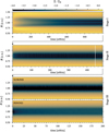 |
Fig. 1 Surface density evolution during the different model stages, normalised by the initial surface density profile. From top to bottom: stage I (2D model), stage II (start of 3D model), and stage III with the NOWIND and PEWIND models, respectively. The white vertical line in the second panel indicates the time at which the model was vertically extended to the final 3D grid (see Sect. 2.3 for details). A black arrow between two panels means that the following stage was started from the end of the previous stage. We note that the scale of the time axis varies between the panels. |
3.1 Surface density structure and evolution
Figure 1 shows the 1D gas surface density evolution for all model stages. It can be seen that in stage one (the initial 2D model), the planet opens up a deep gap over the course of a few hundred orbits. In the middle of the gap, where the planet is located, remains a bump in the surface density from gas accumulating in the circumplanetary region. The surface density reaches a steady state after 600–800 orbits.
After 1000 orbits, we extend the model into three dimensions and start stage II. During the first ≈40 orbits, the surface density adjusts to the new 3D structure before it, too, reaches a steady state. The width and depth of the gap in the 2D and 3D models are similar. After 444 orbits in stage II (marked by the white vertical line in the second panel of Fig. 1), we again extend the domain in the vertical direction to allow the disc wind to be included in the next stage. Since the newly created space is virtually empty with the gas density set to the floor density, the model does not need to adjust, which we verify by running it for another 40 orbits.
In stage III, we activate the gas accretion onto the planet and start another model branch, where the temperature parametrisation described in Sect. 2.3.1 is also active. We refer to the models with and without photoevaporation by the identifiers PEWIND and NOWIND, respectively. In both models, the surface density bump at the planet’s location very quickly disappears as the planet undergoes runaway gas accretion. While there is no change in the width of the gap in either model, in the PEWIND model, the depth of the gap reduces by more than an order of magnitude within fewer than 30 orbits after the start of stage III.
We present the 2D structure of the stage III models in Fig. 2, where it is visible that the reduction of the depth of the gap in the PEWIND model is relatively uniform, almost around the entire azimuth. Only close to the planet, where the gas is following horseshoe orbits, the surface density is lower than in the rest of the gap. Outside the gap, the models remain comparable in their overall disc structure, including the width of the gap and the geometry of the spirals.
In Fig. 3, we present the initial 1d gas surface density profile and the azimuthally averaged surface density profiles at the end of every stage in detail. Comparing the profile of the PEWIND model with that at the end of stage III confirms that the gap has become shallower by a factor of ≈ 10 and even more when we compare it to the NOWIND model, where the gap has been depleted further by the accreting planet. The width of the gap is not affected. Outside the gap, the surface density stays similar between the 3D models, but the PEWIND model exhibits a slightly reduced surface density between approximately 6.5 and 8 au.
Figure 4 shows a 3D representation of the density in the PEWIND model, overlaid with gas streamlines in the disc and wind (white), as well as streamlines that show example paths along which gas can be transported into the planet’s Hill sphere (green). Some paths lead directly through the bound disc, while others lead through the wind onto the planet or into the gap and subsequently onto the planet.
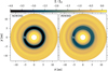 |
Fig. 2 Surface density maps of the NOWIND (left panel) and PEWIND (right panel) models, normalised by the initial surface density profile. The dashed white circle indicates the Hill sphere of the planet. |
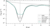 |
Fig. 3 averaged 1D surface density profiles. The dashed grey line indicates the location of the planet. |
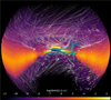 |
Fig. 4 3D visualisation of the density in the PEWIND model created from a snapshot a t = 100 orbits. The dotted lines are gas streamlines. Their colour represents the integration time, which is useful for understanding the direction gas follows along the streamline (from white to green). The cyan tubes are gas streamlines traced back from within the planet’s Hill sphere and indicate example paths that the gas can take towards the planet. |
3.2 Disc structure
In previous work (Weber et al. 2022), we have found that the planetary sub-structures, especially a gap in the disc gas, can profoundly affect the structure and kinematics of a photoevaporative wind. In the presence of a gap, the pressure gradient in the wind-launching region and even beyond the gap is significantly altered, and since a photoevaporative wind is a thermal wind driven by pressure gradient forces, the wind itself is strongly affected, too, which we can also observe in our PEWIND model. In this work, we are mainly interested in the implications of this for the disc and the planet. We only briefly touch upon the impact on the wind and direct readers to our previous work for more details.
In Fig. 5, we show the azimuthally averaged density, pressure and gas temperature structure of the stage III models. The panels in the top row show the density structure, overlaid with density contours that indicate the gap profile. The crucial difference between the models is the heating by EUV + X-ray irradiation from the central star that is applied in the PEWIND model via the temperature parametrisation. The panels in the third row show the resulting temperature structure, overplotted by column density contours up to 2.5 × 1022 cm−2, which is the maximum penetration depth of the X-rays. At the heated surface layers of the disc, the PEWIND model experiences a sharp temperature rise (third row), accompanied by a sharp drop in the gas density, which is in contrast to the NOWIND model, where the density falls off exponentially in the vertical direction. The transition from cold to hot gas can be understood as the transition from the bound disc to the wind-launching region, which happens at column number densities between 2.5 × 10²¹ and 2.5 × 1022 cm−2. A strong pressure gradient develops in this region, pointing away from the disc surface (second row), which can launch a dense wind. However, at the location of the planetary gap, where the density and temperature of the bound disc are low, the pressure is also low. As a result, the pressure gradient is pointing into the gap and no wind is launched from the location of the gap. We discuss the structure of the wind in more detail in the next section.
As seen in the top-right panel, the disc in the PEWIND model has a slightly lower density (by a few percent) radially outside the gap. This can be explained by the mass that has been redistributed or lost due to the wind during the simulation. We can confirm this with a quick estimation: The measured mass-loss rate due to the wind inside the domain is ≈5 × 10⁻⁹ M⊙ yr−1 (see Sect. 3.7 for details). If the mass-loss rate were constant, we would expect to have lost ≈1.42 × 10⁻⁵ M⊙ during our simulation. The difference in total disc mass between the two models is ≈1.37 × 10⁻⁵ M⊙, which corresponds to ≈2.5% of the mass at the start of stage III, consistent with the percent-level difference in the density in the outer disc. Radially inside of the gap, as already noted in the previous section, the gas density is enhanced, and a region of increased density extends radially towards the star into the inner disc down to R ≈ 3 au. A possible explanation could be that a fraction of the surplus gas inside the gap is viscously transported radially inwards. In that case, the planetary gap would be less efficient in blocking the accretion flows towards the star in a model that includes a photoevaporative wind. We discuss the details of this gas redistribution and its implications in the following sections.
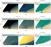 |
Fig. 5 From top to bottom: azimuthally averaged gas density, gas pressure, and gas temperature. From left to right: NOWIND model, PEWIND model, and their relative difference. Dashed white lines are density contours for (from top to bottom) 10−17 to 10−13 g cm−3 in increments of one order of magnitude. Dotted red lines are column density contours for (from top to bottom) 2.5 × 10²⁰, 2.5 × 10²¹, and 2.5 × 1022 cm−2. The arrows in the second row represent the pressure gradient force. In the right column, only the contours of the PEWIND model are shown. The white circles indicate the extent of the planet’s Hill sphere. |
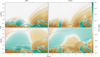 |
Fig. 6 Azimuthally averaged radial and vertical mass flux. The dotted black lines are density contours for (from top to bottom) 10−17 to 10−13 g cm−3 in increments of one order of magnitude. The dashed black circles show the Hill sphere of the planet. The white solid lines are streamlines of the gas. |
3.3 Wind structure and gas redistribution
In Fig. 6, we present the radial and vertical components of the azimuthally averaged mass flux overlaid with the gas streamlines. The kinematic structure of the bound disc is very similar between the models, in agreement with our findings in the previous section that the wind has no significant impact on the bound disc outside of the gap, aside from slight differences in the density. Particularly noteworthy are the meridional circulations that can be seen at the edges of the gap in both models. The only exception is inside the gap above the planet’s Hill sphere, where the PEWIND model has a lot of additional momentum directed radially outwards and downwards, towards the midplane. This momentum is delivered to the gap by the wind. The streamlines demonstrate that the wind is launched from the disc surface everywhere except at the location of the planetary gap. This leads to a zone of low density and pressure in the wind above the gap, causing the pressure gradient in the surrounding wind to point towards that zone. As a result, material that is launched into the wind from the inner disc is driven towards this zone, where it then falls back into the gap, and the same is true for material launched close to the outer edge of the gap. The two flows then collide above the gap’s outer edge, followed by the infall of wind material into the gap. The collision of the opposing flows prevents the direct delivery of gas through the wind across the gap from the inner to the outer disc and vice versa. Instead, mass transport across the gap happens only after the gas is delivered to the gap and subsequently pushed towards the edges by the planet’s torque.
It is important to notice that this effect is entirely dominated by the presence of the gap and its implications on the pressure field and not due to the gravitational potential of the planet, which is negligible at the height of the disc surface. This means that the described behaviour is similar around the entire azimuth and not limited to locations close to the planet.
Above the gap, at heights z ≈ 2 au, is a turning point where the wind turns vertically upwards again. This is further evidence that the wind structure in this region is not significantly affected by reflections at the open polar boundary.
In addition to the gas that is delivered to the gap through the wind, the PEWIND model also has an increased radial and vertical mass flux directly at the gap edges. This can be seen better in the relative difference of the mass flux magnitude within the meridional plane, which we show in Fig. 7, where we marked these regions with yellow ellipses. The increased flux in these regions is likely due to a combination of additional gas delivered by the wind and increased acceleration towards the gap by thermal pressure from the heated disc surface. Moreover, as discussed in the previous section, the gas density is increased in the PEWIND model radially interior to the gap. Consequently, the inner meridional flow carries more mass than in the NOWIND model, which is delivered into that region. At the outer gap, the opposite effect would be expected, but the decrease in mass is outweighed by the mass delivered through the wind and the enhanced acceleration.
These delivery paths combined result in a significant flux directly above the planet’s corotation region that flows towards the outer edge of the gap and vertically towards the midplane. To quantify the amount of extra mass that is delivered through these pathways, we calculate the mass-flux through a ring surface defined by the red line in Fig. 7. This surface spans across the gap, starting and ending where the 10−15 g cm−3 density contours of both models meet, which roughly coincides with the borders of the region of enhanced mass-flux in the PEWIND model. For the PEWIND model, we find a rate of ṁgap,v ≈ 10.7 MJMyr−1 (≈1.0 × 10⁻⁸ M⊙yr−1) flowing through this surface into the gap, compared to ≈2.l MJ Myr−1 (≈2.0 × 10⁻⁹ M⊙yr−1) in the NOWIND model. We list the most important quantities measured in our models in Table 3. We note that this measurement does not give an accurate picture of the total mass that flows into and out of the gap in both models, as it does not account for flows below this surface. Instead, it serves to estimate the amount of gas delivered from the vertical direction.
Overview of the most important quantities measured in the models.
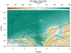 |
Fig. 7 Relative difference of the azimuthally averaged mass flux magnitude in the meridional plane. The dotted black lines are density contours of the PEWIND model for (from top to bottom) 10−17 to 10−13 g cm−3 in increments of one order of magnitude. The dashed grey lines are the same contours for the NOWIND model. The red line defines the ring surface through which we calculate the vertical mass flux into the gap. The solid yellow ellipses highlight the gap edges with increased mass-flux in the PEWIND model. The dashed black circle shows the Hill sphere of the planet. The white solid lines are streamlines of the gas in the PEWIND model. |
3.4 Accretion onto the planet
As discussed in the previous sections, the depth of the planetary gap is reduced in the PEWIND model by more than an order of magnitude. Therefore, the amount of mass available for accretion onto the planet is significantly increased. In Fig. 8, we present the temporal evolution of the accreted mass and the accretion rates onto the planet in both models, measured as the amount of mass removed from inside the Hill sphere, as described in Sect. 2.3.2. After 200 orbits, the planets have accreted 5.6 × 10⁻³ MJ and 11.1 × 10⁻³ MJ in the NOWIND and PEWIND models, respectively. For the mean accretion rate during the last 50 orbits, we measure MP ≈ 1.8 MJ Myr−1 and 4.0 MJ Myr−1, showing that the accretion rate in the PEWIND model is more than twice the rate in the NOWIND model. While significant, this increase in the accretion rate is much lower than the order of magnitude increase in the surface density in the gap. However, as discussed in Sect. 3.1, the density in the gap is not constant along the entire azimuth. It can be seen in Fig. 2 that very close to the planet, the density is lower than far away from the planet. This is because the gas within the coorbital region follows horseshoe orbits and does not necessarily reach the planet’s Hill sphere. In fact, the majority of the gas that reaches the Hill sphere usually does so from the vertical direction (D’Angelo et al. 2003), but the specific dynamics close to the planet and the structure of the circumplanetary disc depend strongly on the thermodynamics in the circumplanetary region (e.g. Szulágyi et al. 2016), which we model only in the very basic manner described in Sect. 2.3.1. Our measured accretion rates can, therefore, only provide a rough approximation. It is nevertheless clear that photoevaporation increases the amount of mass available for accretion.
In the right panel in Fig. 8, it can be seen that the planets in both models accrete with the same rate at the start of stage III, but while in the NOWIND model, the rate quickly drops after the initially available circumplanetary material is accreted, in the PEWIND model, photoevaporation can sustain the initial accretion rate already after only a few orbits before the accretion rate increases to its final value, which is reached after ≈50 orbits.
To study which parts of the disc contribute most to the mass that the planet accretes, we added passive scalars to our simulations, allowing us to trace gas flows and determine the origin of the accreted gas. Starting at orbit 100, we placed 16 passive scalars as tracers in radial bins of 0.5 au width between 2 and 10 au. The bins span the entire vertical extent of the disc. Figure 9 shows the contribution of each radial bin to the accreted mass, the cumulative radial profile, and the fraction that each tracer contributes to the difference of total accreted mass between the models, all evaluated at orbit 150. Since we place the tracers starting only at orbit 100, where there are already density differences between the models, the tracers do not trace the exact same amount of mass between the models. However, this is only significant inside the gap, where the density difference is considerable. To show this, we also present the contribution of the radial bins in the PEWIND model after weighting them by the initially traced mass, which represents the most extreme case and can be considered a limiting case. This is shown as the dashed line in the top panel of Fig. 9. As is evident from the figure, the planet in the PEWIND model can accrete more material than in the NOWIND model from all radial bins up until 9.5 au, beyond which it accretes slightly less than in the NOWIND model. This is consistent with the wind being less efficient at delivering material towards the gap from larger radii outside of the gap because, at large radii, the influence of the gap decreases up until the point where the wind is launched radially outwards again, as would be expected if there was no gap.
A particularly notable difference between the models is the contribution of the bins at R < 3 au: It can be seen from the cumulative profile that in the PEWIND model, ≈3% of the total accreted mass originates inside three au, in contrast to the NOWIND model where there is no significant contribution from inside that radius.
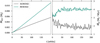 |
Fig. 8 Amount of mass accreted by the planet (left) and mass accretion rates onto the planet (right). |
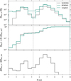 |
Fig. 9 Origin of the mass that was accreted by the planet. Top panel: contribution of the radial bins to the mass accreted by the planet, traced with passive scalars introduced at t = 100 and evaluated at t = 150 orbits. The dashed line shows the profile of the PEWIND model, weighted to account for the discrepancy in the initial amount of mass traced in each bin. Middle panel: cumulative radial profile. Bottom panel: contribution fraction of each radial bin to the additionally accreted mass in the PEWIND model. The grey vertical lines indicate the location of the planet. |
3.5 Planet migration
During our simulations, we also calculated the disc’s gravitational torque that is acting on the planet by integrating over the entire disc, where we followed Crida et al. (2008) and Kley et al. (2009) to apply a tapering function:
![Mathematical equation: ${f_\Gamma }(d) = \left[ {\exp \left( { - {{d/{R_{\rm{H}}} - b} \over {b/10}}} \right)} \right],$](/articles/aa/full_html/2024/06/aa48596-23/aa48596-23-eq16.png) (8)
(8)
with d being the distance from the planet and b = 0.8 a torque cut-off radius in units of RH. This ensures that contributions from gas that is gravitationally bound to the planet are ignored, which is important because, in a more realistic model that does not neglect self-gravity, this gas should experience the same torque as the planet and therefore be considered a part of it. During our analysis of the torques, we used the standard normalisation (Paardekooper et al. 2010):
 (9)
(9)
The left panel of Fig. 10 shows the temporal evolution of the torque. Initially, the magnitude of the torques decreases over time in both models, but the decrease is faster in the PEWIND model. After ≈100 orbits, the torque appears to reach a steady state in the NOWIND model, while it decreases further in the PEWIND model, albeit at a slightly reduced rate. At the end of stage III, the torque in the PEWIND model is reduced almost by a factor of 2. If we assume that the torque remains constant in the NOWIND model, we can estimate the migration timescale as
 (10)
(10)
where Jp is the planet’s angular momentum. Evaluating the timescale for the NOWIND model, we find τM,NOWIND ≈ 5.3 × 10⁵ yr. For the PEWIND model, we find τM,PEWIND ≈ 9.9 × 10⁵ yr; however, the torque will likely continue to decrease in this model, slowing down the migration even more.
As is best visible in the cumulative torque and the radial torque distribution, most of the difference between the models arises between 0.8 and 1.4 ap, which corresponds to 4.16 and 7.28 au, but only a minor contribution comes from inside the corotation region, defined by the extent of the Hill sphere (marked yellow in the figure). The difference can likely be explained by the enhanced density observed radially interior to the gap in the PEWIND model (see Sect. 3.2), leading to a higher positive torque around R = 0.9 ap. The same argument holds the other way around: radially outside the gap, the density is smaller, leading to a weaker negative torque around R = 1.2 ap.
3.6 Mass transport across the gap
The transport of mass across a deep planetary gap can significantly be reduced by an accreting planet, depending on how efficient the planet is in accreting the gas that is supplied from disc (e.g. Lubow & D’Angelo 2006). It was proposed in the past that this could lead to the starvation of the inner disc, resulting in an accelerated dispersal of the inner disc, which could start the transition disc phase, where a photoevaporative wind quickly evaporates away the fully exposed inner edge of the gas cavity (Alexander & Armitage 2009; Rosotti et al. 2013). This process is often called PIPE. Using our 3D models, we can investigate this scenario in full detail, taking into account not only the mass loss but also the redistribution of gas by the wind.
In Fig. 11, we present the mass rates crossing the gap either from the outside in or vice versa. The rates are calculated using our radially binned passive scalar tracers. Gas originating in a particular bin is considered to have crossed the gap if transported across the bin between 5.0 and 5.5 au (shaded in grey in the figure). In the NOWIND model, the total rates of inward and outward transport are ṁcross,in ≈ 2.0 × 10⁻¹⁰ M⊙ yr−1 and ṁcross,out ≈ 6.1 × 10⁻¹¹ M⊙ yr−1, respectively. The PEWIND model has increased rates by factors of 5.4 and 5.1 with 9.9 × 10⁻¹⁰ M⊙ yr−1 and 3.3 × 10⁻¹⁰ M⊙ yr−1, respectively. If we use the simple estimation for the steady state accretion rate onto the star in an unperturbed disc, ṁacc = 3πvΣ with v = αcsH and  , we find ṁacc ≈ 6.6 × 10⁻¹⁰ M⊙ yr−1. This rate is exceeded in the PEWIND model, while in the NOWIND model, only ≈30% of it can be sustained. Moreover, we note that our reported values should be considered lower limits because our tracers are only placed between 2 and 10 au and mass further inside or outside is ignored in this calculation. In particular, this could affect the outward transport rates of the PEWIND model, as the rates are still high for the innermost radial bin between 2 and 2.5 au. Pho-toevaporation usually cannot launch a wind very close to the star (R ⪅ 2 au) because the pressure gradients are not strong enough for the resulting force to overcome the strong gravitational force in the innermost regions of the disc. However, it is nevertheless possible for gas from the inner disc to be pushed outwards along the disc surface and later be picked up by the wind, a process that is facilitated by the presence of a gap that increases the pressure gradient in the radial direction (see also Weber et al. 2022).
In Sect. 3.3, we have seen that the wind cannot deliver material across the gap directly, because it collides with the opposing wind from the other side of the gap, leading to the infall of wind material into the gap. However, the material delivered into the gap can indirectly cross the gap, when the torque from the planet pushes the material towards the edges of the gap, from where it can subsequently diffuse viscously. To provide a more intuitive picture, we visualised the two flows from the outer and inner disc in Appendix B, where we show three different snapshots of the innermost tracer in Fig. B.1 and of a tracer near the outer gap edge in Fig. B.2. Since the disc is viscously accreting onto the star, gas at the outer edge of the gap is not effectively transported farther outwards. Instead, it accumulates at the edge of the gap. In Fig. 12, we show the gas density traced by the tracer originating in our innermost radial bin between 2 and 2.5 au. Between R = 6.5 and 7.5 au, at the location of the meridional flow, the traced gas appears to accumulate, with the tracer density quickly falling off at larger radii.
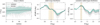 |
Fig. 10 Torque evolution (left panel), radial torque distribution (middle panel), and cumulative radial torque (right panel). The temporal evolution was smoothed with a Gaussian kernel over ten orbits to make the plot more readable, and the shaded area indicates the spread of the actual samples. In the other panels, the shaded area indicates the standard deviation from the mean, calculated from 1000 samples between orbit 190 and 200. The yellow vertical band marks the extent of the planet’s Hill sphere, and horizontal and vertical dashed lines indicate the zero point and the planet’s location, respectively. |
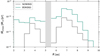 |
Fig. 11 Contribution of the radial bins to the rate of mass crossing the gap either outwards (if to the right of the grey shaded area) or inwards (if to the left of it). |
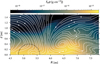 |
Fig. 12 Closeup view of the outer gap edge, showing the density of gas traced by the innermost tracer, i.e. gas that originated between R = 2 and 2.5 au and was transported across the gap. Solid white lines are streamlines, and the dashed black circle indicates the extent of the planet’s Hill sphere. |
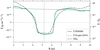 |
Fig. 13 Azimuthally averaged surface mass-loss profile of the PEWIND model. The coloured circles indicate the individual samples and the green solid line is obtained by smoothing the samples using a Gaussian kernel with σ = 3. The dashed black line shows the surface mass-loss profile of the primordial disc by Picogna et al. (2019), which does not have any sub-structures; the vertical dashed line indicates the planet’s location. The dashed-dotted black line shows the 1d surface density profile. |
3.7 Wind mass-loss rate and profile
In Fig. 13, we show the azimuthally averaged surface mass-loss profile in the PEWIND model. The profile was calculated from the mass flux measured through the surface that is 0.4 au above the surface where the temperature gradient reaches its maximum (the transition from blue to yellow in Fig. 5). Consistent with the streamlines discussed in the previous section, the profile shows an infall of mass between 4 and 6.4 au. For comparison, we also show the surface mass-loss profile of the unperturbed primordial disc in Picogna et al. (2019). Although there are differences in the initial conditions between their setup and ours (primarily in disc mass and viscosity), and they use a different method to calculate the mass-loss profiles, the profiles should be robust against these differences since the wind mass-loss profile is mainly dependent on the X-ray spectrum and luminosity, the stellar mass and the disc aspect ratio, all of which we adopted from their model. Indeed, the two profiles reach similar mass-loss rates far away from the planetary gap. The total rate for mass that is lost through this surface (and not falling back) is ṁwind ≈ 5.2 × 10⁻⁹ M⊙ yr−1. However, since the mass-loss close to the domain boundaries can be affected by the wave-dampening we apply, we limit our analysis to the radial range between 2 and 10 au, where the model experiences a wind mass-loss rate of ≈4.1 × 10⁻⁹ M⊙ yr−1. Of that, ≈1.1 × 10⁻⁹ M⊙ yr−1 is lost inside the planet’s orbit. In the same radial range, the surface mass-loss profile of Picogna et al. (2019) yields a rate of ≈6.4 × 10⁻⁹ M⊙ yr−1 of which ≈2.5 × 10⁻⁹ M⊙ yr−1 are lost inside 5.2 au. The total rate for mass falling back into the gap is ≈7.4 × 10⁻¹⁰ M⊙ yr−1. We note that this infall rate only includes gas lifted by at least 0.4 au from the surface and does not include material transported into the gap while staying below that threshold. It is therefore much lower than the rate we found in Sect. 3.3.
4 Discussion
4.1 Inner disc lifetime and PIPE
As shown in the previous sections, a significant fraction of the wind launched from the inner disc is recycled by falling back into the gap and then transported inwards again. In consequence, the wind mass-loss rate in the inner disc is reduced by a factor of ≈2.5 to ≈1.1 × 10⁻⁹ M⊙ yr−1 (see Sect. 3.7). Additionally, due to the increase in mass that is loaded into the gap from outside of the planet’s orbit and then pushed by the planet’s torque towards the edges of the gap, an inward mass transport across the gap is sustained at a rate of ≈10−9 M⊙ yr−1 (see Sect. 3.6). This rate is about 50% higher than the viscous accretion rate in the unperturbed disc despite the presence of a strongly accreting planet. If we assume that all rates remain constant and that the star always accretes gas at the viscous rate, ṁvisc, we can make a simple estimate of the lifetime of the inner disc, τinner:

Minner is the mass of the inner disc. This is, of course, not an accurate estimate. In reality, the rates will not remain constant over the entire lifespan. For example, the accretion rate decreases with decreasing density. But it is still useful for a comparison between the different models. In the case without a planet, we assume that ṁcross,in = ṁvisc, so that the mass accretion rate onto the star balances the resupply from the outer to the inner disc and the inner disc mass decreases with the wind mass-loss rate. The inner disc would then be dispersed after only 80 kyr. In the PEWIND model, the lifetime would be extended by more than a factor of 3 to 260 kyr. In the NOWIND model, the inner disc would be accreted by the star within 455 kyr. If the planetary gap acts as a filter for the dust in the disc, the increased lifetime of the inner gas disc could potentially explain the higher-than-expected occurrence rate of observed accreting transitions discs with large dust cavities (e.g. Ercolano & Pascucci 2017).
The prolonged lifetime of the PEWIND model compared to a model with no planet is opposite to the expectation in the proposed PIPE scenario (Alexander & Armitage 2009; Rosotti et al. 2013), which is based on the assumption that a gap-opening planet reduces the rate of viscous mass-transport to the inner disc. Hydrodynamic simulations show that planets typically reduce the mass flow across the gap to 10–25% of the viscous steady-state accretion rate (Lubow & D’Angelo 2006). Considering the wind recycling and the additional mass-loading across the gap, PIPE can only operate if this reduction exceeds the effects of the wind-driven redistribution, which could be the case for more viscous discs with higher accretion rates.
The effects of the gap on the photoevaporative wind depend primarily on the width of the gap, which increases with increasing orbital radius and decreasing planet-to-star mass ratio, disc scale height and viscosity (Kanagawa et al. 2015). We therefore expect the effects to be more substantial if the disc is less viscous, the planet more massive, or the orbit larger. However, the exact relation between the width of the gap and the size of the affected wind region is unclear because the latter also depends on the temperature and density gradients in the wind itself, which are not scale-invariant so that more models would have to be run to make accurate predictions.
4.2 Observational signatures
In a companion work Weber et al. (2022) studied the effect that the modified wind structure has on the spectral line profiles of forbidden emission lines that are commonly used as disc wind tracers (e.g. O I 6300 Å). They find that while the region above the gap, where the kinematics of the wind is affected the most, is not very well traced by the wind, the asymmetric substructures that are generated by the planet do leave an imprint in the wind that can cause variations in the line profiles that could be observed with high spectral resolution (R ≈ 100 000). Most notably, the peak of the line profiles can move between the blue-and the redshifted parts of the spectrum on timescales of less than a quarter of the planet’s orbit.
In recent years, molecular line observations with ALMA have very successfully been used to detect kinematic signatures of planets via the distortion of the disc’s gas flow (e.g. Pinte et al. 2018; Teague et al. 2019; Wölfer et al. 2023; review by Pinte et al. 2023). In particular, it has become possible to map the 3D gas flow in the vicinity of the planet and, by doing so, to reveal exciting signatures, for example, of meridional flows (e.g. Teague et al. 2019; Yu et al. 2021). Galloway-Sprietsma et al. (2023) even find evidence for an upward flow arising from the location of the gap of AS 209, which could be evidence for a disc wind. In light of these new possibilities, investigating our photoevaporative wind’s effect on these observations would be extremely interesting. Unfortunately, the spatial resolution of the observations currently limits this kind of analysis to planets at larger separations than that in our model. However, we present in a future work synthetic observations of our model with a planet at a larger distance from the star to investigate the effect that photoevaporation has on the kinematic signatures of the planet.
One of our main findings in this work is that the photoe-vaporative wind refills the gap, reducing its depth by more than an order of magnitude. This possibility should be considered when inferring disc or planet properties, such as the viscosity parameter α or the planet’s mass from observed gap depths (e.g. Kanagawa et al. 2015; Liu et al. 2018).
4.3 Mixing and reprocessing of disc material
Our results show that a photoevaporative wind can redistribute material from the inner disc towards the gap and the circum-planetary region, from where it can be accreted by the planet or accumulate near the meridional flows at the gap edges. This could have significant consequences on the gas composition near the gap or in the planet’s atmosphere because the gas in the inner disc is expected to have a different composition than that in the outer disc. For example, inward drifting and evaporating pebbles can significantly enrich the inner disc with volatile vapour (e.g. H2O inside the water snow line; Booth et al. 2017; Schneider & Bitsch 2021). If it is then transported through the wind towards the planet, this could enrich the planet’s atmosphere with heavy elements, even if the planet is located beyond the respective snow lines of the volatiles. Such enrichment is not only observed for most hot-Jupiters (Thorngren et al. 2016) but also for the giant planets in the Solar System, which all have an enhanced heavy element mass-fraction compared to the solar value (e.g. review by Guillot et al. 2023).
It should also be considered that when gas or dust is transported through the wind or along the disc surface, it is subject to a high-temperature environment with highly energetic EUV or X-ray irradiation from the central star. This allows for a reprocessing of the material that is impossible in the disc’s interior. one such process is isotope selective photodissociation, an essential mechanism for isotope fractionation, especially for oxygen and nitrogen isotopes (Visser et al. 2009; Furuya & Aikawa 2018; review by Nomura et al. 2023). Isotopic ratios are valuable tools for tracing the chemical evolution and origin of objects in our Solar System. However, to link them to planetary formation theories, it is necessary to take into account the environment that the gas and dust were already subject to in the protoplanetary disc.
Besides the gas, photoevaporation could also help redistribute small dust grains in the disc. Using the same photoevap-oration model as in our model, Franz et al. (2020, 2022) find that the photoevaporative wind can entrain dust grains with a size of up to ≈11 µm. This depends strongly on the amount of small grains that are available on the disc surface, and thus on the degree of vertical mixing in the disc, for example, by the vertical shear instability (e.g. Flock et al. 2017, 2020). In Sect. 3.3, we have also seen that the meridional flows, where some of the redistributed material accumulates, contribute significantly to mass delivery into the gap. They could also stir up dust grains from the midplane towards the surface, where they could undergo further reprocessing.
Addressing the above points will require the detailed postprocessing of our model to calculate the chemical evolution of the gas and, ideally, the dust. While this is beyond the scope of this work, the model presented here can serve as the basis for future investigations.
4.4 Comparison with magnetic wind models
Several studies that have been published recently have investigated the interplay between planet-hosting discs and magnetic winds. In particular, Aoyama & Bai (2023) and Wafflard-Fernandez & Lesur (2023) independently find that the magnetic field lines concentrate in the gap and are deflected by the planet such that a magnetic wind is driven most dominantly from the outer edge of the gap. This is in contrast to our findings with a photoevaporative wind, which promotes a vertical infall into the gap also at the outer edge. As we find in our model, Wafflard-Fernandez & Lesur (2023) report reduced migration rates of the planet in the presence of an MHD wind, a result of their gap becoming asymmetric with the outer gap being deeper radially outside of the planet than inside. Aoyama & Bai (2023) also find that the gaps become deeper and wider in their MHD simulations.
It is likely that, in reality, disc winds are not either purely magnetic or purely thermal, but both mechanisms operate simultaneously, and their relative importance may vary with the evolutionary stage of the disc (e.g. Pascucci et al. 2020). In that case, a magnetic wind could act against the infall of a thermal component in the wind if it is strong enough to overcome the inverted thermal pressure gradient and sustain the wind above the gap. However, if the magnetic wind cannot completely prevent the infall, some of the effects observed in both models could amplify each other. For instance, the reduced migration rate is observed with both types of winds. It is also expected that with wider gaps, a larger volume of the wind is affected. Wind models that combine both (non-ideal) MHD effects and photoevaporation currently exist only for 2D axisymmetric discs without planets, but they still provide very useful insights into the wind-launching processes.
Wang et al. (2019) developed non-ideal MHD disc wind models including self-consistent thermochemistry. They find that their magneto-thermal wind is predominantly launched by the magnetic toroidal pressure gradient and that radiative heating affects the wind launching only weakly, although the mass-loss rate of their wind depends on the ionisation fraction near the wind base and is thus moderately affected by the luminosity of high-energy radiation, mainly soft far-ultraviolet (FUV) and Lyman-Werner photons. In their model, the X-ray luminosity affects the accretion rate rather than the wind mass-loss rate. However, they only include 3 keV X-ray photons, and as was shown by Ercolano et al. (2009), the heating in the wind-launching region is by far dominated by the soft X-ray band (<1 keV). In a similar model with more complete radiation physics (but still mainly focused on FUV-driven processes), Gressel et al. (2020) find a wind that is launched magneto-centrifugally rather than by magnetic toroidal pressure, so the mass loss is also only moderately affected by thermochemical effects. In both cases, the dynamics of the magnetic wind do not depend strongly on the thermal pressure, and its behaviour in the presence of a gap would depend on the impact of the gap on the magnetic field.
Other models indicate that thermal pressure may play an important role even in the presence of a magneto-thermal wind: Rodenkirch et al. (2020) modelled a wind that includes ohmic diffusion as a non-ideal MHD effect and implements the same temperature and ionisation parametrisation by Picogna et al. (2019) that is used in this work. They find that photoevapora-tion is the dominant launching mechanism for weak magnetic fields with a plasma parameter β > 107. With a different model that includes all non-ideal MHD effects and again the same temperature parametrisation, Sarafidou et al. (2024) find that while the inner regions of the disc (R ≤ 1.5 au) are always dominated by magnetic winds, photoevaporation can dominate the mass loss at larger radii for stronger magnetic fields (β ≥ 105 or even stronger), depending on the X-ray luminosity. Moreover, they find that beyond the footpoint of the wind, it is generally sustained thermally rather than magnetically. In that case, the thermal pressure may dominate over the magnetic field in the region above the gap where the pressure gradient is inverted, such that the infall is sustained against the magnetic wind, especially from the inner disc, considering the magnetic wind is expected to be weaker at the inner edge of the gap. However, without detailed models of non-ideal magneto-thermal winds in protoplanetary discs with gaps, the outcome of this scenario remains unclear.
5 Summary
We have performed 3D radiation-hydrodynamic simulations of a photoevaporating, viscous (α = 6.9 × 10⁻⁴) protoplanetary disc hosting a Jupiter-like planet. We studied the interplay between the photoevaporative wind and the sub-structures generated by the planet, particularly the gap, and traced the redistribution of the gas and its accretion onto the planet. For comparison, we also ran the model with photoevaporation switched off. We refer to the models with and without photoevaporation with the identifiers PEWIND and NOWIND, respectively. Our results show that:
At the location of the gap carved by the planet, a photoevap-orative wind cannot be supported. In the vicinity of the gap, the pressure gradient in the wind is inverted, and the wind falls back into the gap. Consequently, the depth of the gap is reduced by more than an order of magnitude. The same mechanism is at work not only in the wind but also at the hot, uppermost layers of the disc surface at the inner and outer edge of the gap;
The continuous resupply of gas into the gap significantly increases the amount of mass the planet has available for accretion. In our simplified accretion model, this leads to a factor of 2 increase in the planet’s accretion rate. Most of the additionally accreted gas originates from a radius up to ≈8 au, beyond which the wind structure is not significantly affected by the presence of the gap. It is particularly noteworthy that ≈3 percent of the accreted mass originates inside R < 3 au if photoevaporation is operating. In the NOWIND model, this region does not significantly contribute to the accreted mass;
The modified density structure of the disc leads to a reduction in the torque that is acting on the planet. After 200 orbits, the migration timescale is already reduced by almost a factor of 2 compared to the case without pho-toevaporation, and the torque is expected to continue to decrease;
After being delivered to the gap, the material that is not accreted by the planet is pushed towards the edges of the gap by the gravitational torque of the planet, from where it viscously diffuses in the bound disc. This leads to an increase in the gap-crossing rates by a factor of ≈5 in both directions compared to the NOWIND model. Consequently, the rate of mass crossing the gap from the outer disc to the inner disc in the PEWIND model is higher than the viscous accretion rate that would be expected in an unperturbed disc without a planet;
The increased inward crossing rate, in combination with the recycling of a significant portion of the wind that is falling back to the gap, results in a slower dispersal and, therefore, a longer lifetime for the inner disc compared to a model without a planet. This is opposite to the PIPE scenario that has been proposed in the past.
The wind-driven redistribution of gas could potentially influence the chemical and isotopic composition of the planet’s atmosphere and the material in the vicinity of the gap. In future work, we will present an adapted model more suitable for creating synthetic observations of molecular (CO) emissions and compare them to actual observations. It is unclear how a magnetic wind would change our results. Models of non-ideal magneto-thermal winds in protoplanetary discs with gaps will be valuable for determining whether an infall would also happen in the presence of magnetic fields.
Acknowledgements
We would like to thank the anonymous referee for a constructive report that improved the manuscript. This research was supported by the Excellence Cluster ORIGINS, which is funded by the Deutsche Forschungsge-meinschaft (DFG, German Research Foundation) under Germany’s Excellence Strategy — EXC-2094-390783311. GP and BE acknowledge the support of the Deutsche Forschungsgemeinschaft (DFG, German Research Foundation) – 325594231. The simulations have been carried out on the computing facilities of the Computational Center for Particle and Astrophysics (C2PAP).
Appendix A Influence of the diffuse EUV and X-ray field on the temperature structure of the gap
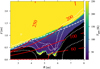 |
Fig. A.1 Temperature structure of a density slice at Φ = 0 post-processed with MOCASSIN. The dashed white line shows the contour for a column number density of 2.5 × 1022 cm−2, above which the temperature is fixed to the dust temperature. The red solid lines are contours of the dust temperature. The dotted white lines are density contours for (from top to bottom) 10−16 to 10−13 g cm−3 in increments of one order of magnitude and indicate the structure of the gap. The black region is too far inside the disc to receive any energy packets in the radiative transfer calculation, which means it is shielded from stellar radiation or the diffuse field. |
A shortcoming of the temperature parametrisation used in our models is that any heating by diffuse EUV or X-ray radiation is neglected. To verify that this effect is not strong enough to affect our result significantly, we took a density slice of our model at Φ = 0 in the Rθ plane and post-processed it with MOCASSIN, using the same configuration as was used by Picogna et al. (2019) to derive the parametrisation. We present the resulting temperature structure inside the gap in Fig. A.1. Most of the gap is not significantly heated by the diffuse field, and the temperature remains below the dust temperature. In our model, the dust temperature is assumed where the column number density exceeds 2.5 × 1022 cm−2. Hence, the diffuse field has only an effect if it can heat the gas beyond the dust temperature. This is the case only deep inside the gap, close to the 10−14 g cm−3 density contour, where the temperature reaches up to ≈250 K. However, this temperature and the resulting pressure gradient are more than an order of magnitude lower than the opposing gradient at the surface of the disc and not sufficient to launch a photoevapora-tive wind inside the gap. We can illustrate this using the basic concept of the gravitational radius (Liffman 2003),
 (A.1)
(A.1)
which is often used to approximate the radius outside of which a photoevaporative wind can be launched. Here, mp is the proton mass, kB is the Boltzmann constant, and T is the gas temperature. For T = 250 K, we find Rg ≈ 100 au, much larger than the radius of the gap.
Appendix B Snapshots of gas tracers
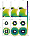 |
Fig. B.1 Poloidal mass flux of the gas originating in the innermost radial tracer bin between R = 2 and 2.5 au at t = 5, 25, and 50 orbits. The top panels show the azimuthal average, and the bottom panels show the traced mass flux in the midplane. The dotted black lines are density contours for (from top to bottom) 10−17 to 10−13 g/cm3 in increments of one order of magnitude. The red circle indicates the extent of the planet’s Hill sphere. The dashed grey lines show the boundaries of the radial bin, inside of which the tracer was originally distributed. |
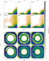 |
Fig. B.2 Same as Fig. B.1 but for the tracer that originates in the radial bin between R = 6 and 6.5 au |
References
- Alexander, R. D., & Armitage, P. J. 2009, ApJ, 704, 989 [Google Scholar]
- Alexander, R. D., & Pascucci, I. 2012, MNRAS, 422, L82 [NASA ADS] [CrossRef] [Google Scholar]
- Alexander, R. D., Clarke, C. J., & Pringle, J. E. 2006, MNRAS, 369, 229 [CrossRef] [Google Scholar]
- Aoyama, Y., & Bai, X.-N. 2023, ApJ, 946, 5 [NASA ADS] [CrossRef] [Google Scholar]
- Asplund, M., Grevesse, N., & Sauval, A. J. 2005, Cosmic Abundances as Records of Stellar Evolution and Nucleosynthesis, 336, 25 [NASA ADS] [Google Scholar]
- Bai, X.-N., Ye, J., Goodman, J., & Yuan, F. 2016, ApJ, 818, 152 [Google Scholar]
- Benítez-Llambay, P., & Masset, F. S. 2016, ApJS, 223, 11 [Google Scholar]
- Béthune, W., Lesur, G., & Ferreira, J. 2017, A&A, 600, A75 [NASA ADS] [CrossRef] [EDP Sciences] [Google Scholar]
- Booth, R. A., Clarke, C. J., Madhusudhan, N., & Ilee, J. D. 2017, MNRAS, 469, 3994 [Google Scholar]
- Crida, A., Sándor, Z., & Kley, W. 2008, A&A, 483, 325 [NASA ADS] [CrossRef] [EDP Sciences] [Google Scholar]
- D’Alessio, P., Calvet, N., & Hartmann, L. 2001, ApJ, 553, 321 [Google Scholar]
- D’Angelo, G., & Lubow, S. H. 2008, ApJ, 685, 560 [CrossRef] [Google Scholar]
- D’Angelo, G., Kley, W., & Henning, T. 2003, ApJ, 586, 540 [Google Scholar]
- De Val-Borro, M., Edgar, R. G., Artymowicz, P., et al. 2006, MNRAS, 370, 529 [NASA ADS] [CrossRef] [Google Scholar]
- Dürmann, C., & Kley, W. 2017, A&A, 598, 80 [Google Scholar]
- Elbakyan, V., Wu, Y., Nayakshin, S., & Rosotti, G. 2022, MNRAS, 515, 3113 [NASA ADS] [CrossRef] [Google Scholar]
- Ercolano, B., & Owen, J. E. 2010, MNRAS, 406, 1553 [NASA ADS] [Google Scholar]
- Ercolano, B., & Owen, J. E. 2016, MNRAS, 460, 3472 [Google Scholar]
- Ercolano, B., & Pascucci, I. 2017, Roy. Soc. Open Sci., 4, 170114 [Google Scholar]
- Ercolano, B., & Picogna, G. 2022, Eur. Phys. J. Plus, 137, 1357 [NASA ADS] [CrossRef] [Google Scholar]
- Ercolano, B., & Rosotti, G. 2015, MNRAS, 450, 3008 [Google Scholar]
- Ercolano, B., Barlow, M. J., Storey, P. J., & Liu, X. W. 2003, MNRAS, 340, 1136 [Google Scholar]
- Ercolano, B., Barlow, M. J., & Storey, P. J. 2005, MNRAS, 362, 1038 [Google Scholar]
- Ercolano, B., Drake, J. J., Raymond, J. C., & Clarke, C. C. 2008a, ApJ, 688, 398 [Google Scholar]
- Ercolano, B., Young, P. R., Drake, J. J., & Raymond, J. C. 2008b, ApJS, 175, 534 [NASA ADS] [CrossRef] [Google Scholar]
- Ercolano, B., Clarke, C. J., & Drake, J. J. 2009, ApJ, 699, 1639 [Google Scholar]
- Ercolano, B., Koepferl, C., Owen, J., & Robitaille, T. 2015, MNRAS, 452, 3689 [NASA ADS] [CrossRef] [Google Scholar]
- Ercolano, B., Picogna, G., & Monsch, K. 2023, MNRAS, 526, L105 [NASA ADS] [CrossRef] [Google Scholar]
- Fedele, D., Van Den Ancker, M. E., Henning, T., Jayawardhana, R., & Oliveira, J. M. 2010, A&A, 510, A72 [NASA ADS] [CrossRef] [EDP Sciences] [Google Scholar]
- Flock, M., Nelson, R. P., Turner, N. J., et al. 2017, ApJ, 850, 131 [Google Scholar]
- Flock, M., Turner, N. J., Nelson, R. P., et al. 2020, ApJ, 897, 155 [Google Scholar]
- Franz, R., Picogna, G., Ercolano, B., & Birnstiel, T. 2020, A&A, 635, A53 [EDP Sciences] [Google Scholar]
- Franz, R., Ercolano, B., Casassus, S., et al. 2022, A&A, 657, A69 [NASA ADS] [CrossRef] [EDP Sciences] [Google Scholar]
- Fung J. & Chiang E. 2016 ApJ 832 105 [NASA ADS] [CrossRef] [Google Scholar]
- Furuya, K., & Aikawa, Y. 2018, ApJ, 857, 105 [Google Scholar]
- Galloway-Sprietsma, M., Bae, J., Teague, R., et al. 2023, ApJ, 950, 147 [NASA ADS] [CrossRef] [Google Scholar]
- Goldreich, P., & Tremaine, S. 1979, ApJ, 233, 857 [Google Scholar]
- Goldreich, P., & Tremaine, S. 1980, ApJ, 241, 425 [Google Scholar]
- Gorti, U., & Hollenbach, D. 2009, ApJ, 690, 1539 [Google Scholar]
- Gressel, O., Turner, N. J., Nelson, R. P., & McNally, C. P. 2015, ApJ, 801, 84 [NASA ADS] [CrossRef] [Google Scholar]
- Gressel, O., Ramsey, J. P., Brinch, C., et al. 2020, ApJ, 896, 126 [Google Scholar]
- Guillot, T., Fletcher, L. N., Helled, R., et al. 2023, ASP Conf. Ser., 534, 947, Protostars and Planets VII, eds. S. Inutsuka, Y. Aikawa, T. Muto, K. Tomida, & M. Tamura [Google Scholar]
- Haisch, K. E., Jr., Lada, E. A., & Lada, C. J. 2001, ApJ, 553, L153 [NASA ADS] [CrossRef] [Google Scholar]
- Jennings, J., Ercolano, B., & Rosotti, G. P. 2018, MNRAS, 477, 4131 [Google Scholar]
- Kanagawa, K. D., Muto, T., Tanaka, H., et al. 2015, ApJ, 806, L15 [NASA ADS] [CrossRef] [Google Scholar]
- Kimmig, C. N., Dullemond, C. P., & Kley, W. 2020, A&A, 633, A4 [NASA ADS] [CrossRef] [EDP Sciences] [Google Scholar]
- Klahr, H., & Kley, W. 2006, A&A, 445, 747 [NASA ADS] [CrossRef] [EDP Sciences] [Google Scholar]
- Kley, W., & Nelson, R. P. 2012, ArA&A, 50, 211 [NASA ADS] [CrossRef] [Google Scholar]
- Kley, W., Bitsch, B., & Klahr, H. 2009, A&A, 506, 971 [NASA ADS] [CrossRef] [EDP Sciences] [Google Scholar]
- Koepferl, C. M., Ercolano, B., Dale, J., et al. 2013, MNRAS, 428, 3327 [Google Scholar]
- Lega, E., Nelson, R. P., Morbidelli, A., et al. 2021, A&A, 646, A166 [NASA ADS] [CrossRef] [EDP Sciences] [Google Scholar]
- Lesur, G. R. 2021, A&A, 650, A35 [NASA ADS] [CrossRef] [EDP Sciences] [Google Scholar]
- Lesur, G., Flock, M., Ercolano, B., et al. 2023, ASP Conf. Ser., 534, 465, Protostars and Planets VII, eds. S. Inutsuka, Y. Aikawa, T. Muto, K. Tomida, & M. Tamura [NASA ADS] [Google Scholar]
- Liffman, K. 2003, PASA, 20, 337 [NASA ADS] [CrossRef] [Google Scholar]
- Liu, S.-F., Jin, S., Li, S., Isella, A., & Li, H. 2018, ApJ, 857, 87 [NASA ADS] [CrossRef] [Google Scholar]
- Lubow, S. H., & D’Angelo, G. 2006, ApJ, 641, 526 [Google Scholar]
- Mamajek, E. E., Usuda, T., Tamura, M., & Ishii, M. 2009, in EXOPLANETS AND DISKS : THEIR FORMATION AND DIVERSITY: Proceedings of the International Conference, AIP Conf. Proc. 1158, 3 [NASA ADS] [CrossRef] [Google Scholar]
- Masset, F. 2000, A&AS, 141, 165 [NASA ADS] [CrossRef] [EDP Sciences] [Google Scholar]
- Mignone, A., Bodo, G., Massaglia, S., et al. 2007, ApJS, 170, 228 [Google Scholar]
- Monsch, K., Ercolano, B., Picogna, G., Preibisch, T., & Rau, M. M. 2019, MNRAS, 483, 3448 [Google Scholar]
- Monsch, K., Picogna, G., Ercolano, B., & Kley, W. 2021a, A&A, 646, A169 [NASA ADS] [CrossRef] [EDP Sciences] [Google Scholar]
- Monsch, K., Picogna, G., Ercolano, B., & Preibisch, T. 2021b, A&A, 650, A199 [NASA ADS] [CrossRef] [EDP Sciences] [Google Scholar]
- Morbidelli, A., Szulágyi, J., Crida, A., et al. 2014, Icarus, 232, 266 [Google Scholar]
- Nelson, R. P., Gressel, O., & Umurhan, O. M. 2013, MNRAS, 435, 2610 [Google Scholar]
- Nelson, R. P., Lega, E., & Morbidelli, A. 2023, A&A, 670, A113 [NASA ADS] [CrossRef] [EDP Sciences] [Google Scholar]
- Nomura, H., Furuya, K., Cordiner, M. A., et al. 2023, ASP Conf. Ser., 534, 1075, Protostars and Planets VII, eds. S. Inutsuka, Y. Aikawa, T. Muto, K. Tomida, & M. Tamura [NASA ADS] [Google Scholar]
- Owen, J. E., Ercolano, B., Clarke, C. J., & Alexander, R. D. 2010, MNRAS, 401, 1415 [Google Scholar]
- Paardekooper, S. J., Baruteau, C., Crida, A., & Kley, W. 2010, MNRAS, 401, 1950 [NASA ADS] [CrossRef] [Google Scholar]
- Paardekooper, S., Dong, R., Duffell, P., et al. 2023, ASP Conf. Ser., 534, 685, Protostars and Planets VII, eds. S. Inutsuka, Y. Aikawa, T. Muto, K. Tomida, & M. Tamura [NASA ADS] [Google Scholar]
- Papaloizou, J., & Lin, D. N. C. 1984, ApJ, 285, 818 [NASA ADS] [CrossRef] [Google Scholar]
- Pascucci, I., Banzatti, A., Gorti, U., et al. 2020, ApJ, 903, 78 [Google Scholar]
- Pascucci, I., Cabrit, S., Edwards, S., et al. 2023, ASP Conf. Ser., 534, 567, Protostars and Planets VII, eds. S. Inutsuka, Y. Aikawa, T. Muto, K. Tomida, & M. Tamura [NASA ADS] [Google Scholar]
- Picogna, G., Ercolano, B., Owen, J. E., & Weber, M. L. 2019, MNRAS, 487, 691 [Google Scholar]
- Pinte, C., Price, D. J., Ménard, F., et al. 2018, ApJ, 860, L13 [Google Scholar]
- Pinte, C., Teague, R., Flaherty, K., et al. 2023, ASP Conf. Ser., 534, 645, Protostars and Planets VII, eds. S. Inutsuka, Y. Aikawa, T. Muto, K. Tomida, & M. Tamura [NASA ADS] [Google Scholar]
- Rab, Ch., Weber, M., Grassi, T., et al. 2022, A&A, 668, A154 [NASA ADS] [CrossRef] [EDP Sciences] [Google Scholar]
- Rab, C., Weber, M. L., Picogna, G., Ercolano, B., & Owen, J. E. 2023, ApJ, 955, L11 [NASA ADS] [CrossRef] [Google Scholar]
- Ribas, Á., Merín, B., Bouy, H., & Maud, L. T. 2014, A&A, 561, A54 [NASA ADS] [CrossRef] [EDP Sciences] [Google Scholar]
- Rodenkirch, P. J., Klahr, H., Fendt, C., & Dullemond, C. P. 2020, A&A, 633, A21 [NASA ADS] [CrossRef] [EDP Sciences] [Google Scholar]
- Rosotti, G. P., Ercolano, B., Owen, J. E., & Armitage, P. J. 2013, MNRAS, 430, 1392 [Google Scholar]
- Sarafidou, E., Gressel, O., Picogna, G., & Ercolano, B. 2024, MNRAS, 530, 5131 [NASA ADS] [CrossRef] [Google Scholar]
- Savage, B. D., & Sembach, K. R. 1996, ApJ, 470, 893 [Google Scholar]
- Schneider, A. D., & Bitsch, B. 2021, A&A, 654, A71 [Google Scholar]
- Shakura, N. I., & Sunyaev, R. A. 1973, A&A, 24, 337 [NASA ADS] [Google Scholar]
- Szulágyi, J. 2017, ApJ, 842, 103 [Google Scholar]
- Szulágyi, J., Masset, F., Lega, E., et al. 2016, MNRAS, 460, 2853 [Google Scholar]
- Teague, R., Bae, J., & Bergin, E. A. 2019, Nature, 574, 378 [NASA ADS] [CrossRef] [Google Scholar]
- Thorngren, D. P., Fortney, J. J., Murray-Clay, R. A., & Lopez, E. D. 2016, ApJ, 831, 64 [NASA ADS] [CrossRef] [Google Scholar]
- Visser, R., van Dishoeck, E. F., & Black, J. H. 2009, A&A, 503, 323 [NASA ADS] [CrossRef] [EDP Sciences] [Google Scholar]
- Wafflard-Fernandez, G., & Lesur, G. 2023, A&A, 677, A70 [NASA ADS] [CrossRef] [EDP Sciences] [Google Scholar]
- Wang, L., Bai, X.-N., & Goodman, J. 2019, ApJ, 874, 90 [Google Scholar]
- Weber, M. L., Ercolano, B., Picogna, G., Hartmann, L., & Rodenkirch, P. J. 2020, MNRAS, 496, 223 [NASA ADS] [CrossRef] [Google Scholar]
- Weber, M. L., Ercolano, B., Picogna, G., & Rab, C. 2022, MNRAS, 517, 3598 [NASA ADS] [CrossRef] [Google Scholar]
- Wölfer, L., Facchini, S., van der Marel, N., et al. 2023, A&A, 670, A154 [CrossRef] [EDP Sciences] [Google Scholar]
- Yu, H., Teague, R., Bae, J., & Oberg, K. 2021, ApJ, 920, L33 [NASA ADS] [CrossRef] [Google Scholar]
All Tables
All Figures
|
Fig. 1 Surface density evolution during the different model stages, normalised by the initial surface density profile. From top to bottom: stage I (2D model), stage II (start of 3D model), and stage III with the NOWIND and PEWIND models, respectively. The white vertical line in the second panel indicates the time at which the model was vertically extended to the final 3D grid (see Sect. 2.3 for details). A black arrow between two panels means that the following stage was started from the end of the previous stage. We note that the scale of the time axis varies between the panels. |
| In the text | |
|
Fig. 2 Surface density maps of the NOWIND (left panel) and PEWIND (right panel) models, normalised by the initial surface density profile. The dashed white circle indicates the Hill sphere of the planet. |
| In the text | |
|
Fig. 3 averaged 1D surface density profiles. The dashed grey line indicates the location of the planet. |
| In the text | |
|
Fig. 4 3D visualisation of the density in the PEWIND model created from a snapshot a t = 100 orbits. The dotted lines are gas streamlines. Their colour represents the integration time, which is useful for understanding the direction gas follows along the streamline (from white to green). The cyan tubes are gas streamlines traced back from within the planet’s Hill sphere and indicate example paths that the gas can take towards the planet. |
| In the text | |
|
Fig. 5 From top to bottom: azimuthally averaged gas density, gas pressure, and gas temperature. From left to right: NOWIND model, PEWIND model, and their relative difference. Dashed white lines are density contours for (from top to bottom) 10−17 to 10−13 g cm−3 in increments of one order of magnitude. Dotted red lines are column density contours for (from top to bottom) 2.5 × 10²⁰, 2.5 × 10²¹, and 2.5 × 1022 cm−2. The arrows in the second row represent the pressure gradient force. In the right column, only the contours of the PEWIND model are shown. The white circles indicate the extent of the planet’s Hill sphere. |
| In the text | |
|
Fig. 6 Azimuthally averaged radial and vertical mass flux. The dotted black lines are density contours for (from top to bottom) 10−17 to 10−13 g cm−3 in increments of one order of magnitude. The dashed black circles show the Hill sphere of the planet. The white solid lines are streamlines of the gas. |
| In the text | |
|
Fig. 7 Relative difference of the azimuthally averaged mass flux magnitude in the meridional plane. The dotted black lines are density contours of the PEWIND model for (from top to bottom) 10−17 to 10−13 g cm−3 in increments of one order of magnitude. The dashed grey lines are the same contours for the NOWIND model. The red line defines the ring surface through which we calculate the vertical mass flux into the gap. The solid yellow ellipses highlight the gap edges with increased mass-flux in the PEWIND model. The dashed black circle shows the Hill sphere of the planet. The white solid lines are streamlines of the gas in the PEWIND model. |
| In the text | |
|
Fig. 8 Amount of mass accreted by the planet (left) and mass accretion rates onto the planet (right). |
| In the text | |
|
Fig. 9 Origin of the mass that was accreted by the planet. Top panel: contribution of the radial bins to the mass accreted by the planet, traced with passive scalars introduced at t = 100 and evaluated at t = 150 orbits. The dashed line shows the profile of the PEWIND model, weighted to account for the discrepancy in the initial amount of mass traced in each bin. Middle panel: cumulative radial profile. Bottom panel: contribution fraction of each radial bin to the additionally accreted mass in the PEWIND model. The grey vertical lines indicate the location of the planet. |
| In the text | |
|
Fig. 10 Torque evolution (left panel), radial torque distribution (middle panel), and cumulative radial torque (right panel). The temporal evolution was smoothed with a Gaussian kernel over ten orbits to make the plot more readable, and the shaded area indicates the spread of the actual samples. In the other panels, the shaded area indicates the standard deviation from the mean, calculated from 1000 samples between orbit 190 and 200. The yellow vertical band marks the extent of the planet’s Hill sphere, and horizontal and vertical dashed lines indicate the zero point and the planet’s location, respectively. |
| In the text | |
|
Fig. 11 Contribution of the radial bins to the rate of mass crossing the gap either outwards (if to the right of the grey shaded area) or inwards (if to the left of it). |
| In the text | |
|
Fig. 12 Closeup view of the outer gap edge, showing the density of gas traced by the innermost tracer, i.e. gas that originated between R = 2 and 2.5 au and was transported across the gap. Solid white lines are streamlines, and the dashed black circle indicates the extent of the planet’s Hill sphere. |
| In the text | |
|
Fig. 13 Azimuthally averaged surface mass-loss profile of the PEWIND model. The coloured circles indicate the individual samples and the green solid line is obtained by smoothing the samples using a Gaussian kernel with σ = 3. The dashed black line shows the surface mass-loss profile of the primordial disc by Picogna et al. (2019), which does not have any sub-structures; the vertical dashed line indicates the planet’s location. The dashed-dotted black line shows the 1d surface density profile. |
| In the text | |
|
Fig. A.1 Temperature structure of a density slice at Φ = 0 post-processed with MOCASSIN. The dashed white line shows the contour for a column number density of 2.5 × 1022 cm−2, above which the temperature is fixed to the dust temperature. The red solid lines are contours of the dust temperature. The dotted white lines are density contours for (from top to bottom) 10−16 to 10−13 g cm−3 in increments of one order of magnitude and indicate the structure of the gap. The black region is too far inside the disc to receive any energy packets in the radiative transfer calculation, which means it is shielded from stellar radiation or the diffuse field. |
| In the text | |
|
Fig. B.1 Poloidal mass flux of the gas originating in the innermost radial tracer bin between R = 2 and 2.5 au at t = 5, 25, and 50 orbits. The top panels show the azimuthal average, and the bottom panels show the traced mass flux in the midplane. The dotted black lines are density contours for (from top to bottom) 10−17 to 10−13 g/cm3 in increments of one order of magnitude. The red circle indicates the extent of the planet’s Hill sphere. The dashed grey lines show the boundaries of the radial bin, inside of which the tracer was originally distributed. |
| In the text | |
|
Fig. B.2 Same as Fig. B.1 but for the tracer that originates in the radial bin between R = 6 and 6.5 au |
| In the text | |
Current usage metrics show cumulative count of Article Views (full-text article views including HTML views, PDF and ePub downloads, according to the available data) and Abstracts Views on Vision4Press platform.
Data correspond to usage on the plateform after 2015. The current usage metrics is available 48-96 hours after online publication and is updated daily on week days.
Initial download of the metrics may take a while.