| Issue |
A&A
Volume 686, June 2024
|
|
|---|---|---|
| Article Number | A79 | |
| Number of page(s) | 30 | |
| Section | Extragalactic astronomy | |
| DOI | https://doi.org/10.1051/0004-6361/202347883 | |
| Published online | 30 May 2024 | |
The carbon-rich type Ic supernova 2016adj in the iconic dust lane of Centaurus A: Potential signatures of an interaction with circumstellar hydrogen⋆,⋆⋆
1
Department of Physics and Astronomy, Aarhus University, Ny Munkegade 120, 8000 Aarhus C, Denmark
e-mail: This email address is being protected from spambots. You need JavaScript enabled to view it.
2
Planetary Science Institute, 1700 E Fort Lowell Rd., Ste 106, Tucson, AZ 85719, USA
3
Hamburger Sternwarte, Gojensbergweg 112, 21029 Hamburg, Germany
4
Observatories of the Carnegie Institution for Science, 813 Santa Barbara St., Pasadena, CA 91101, USA
5
School of Physics, O’Brien Centre for Science North, University College Dublin, Belfield, Dublin 4, Ireland
6
Institute of Space Sciences (ICE, CSIC), Campus UAB, Carrer de Can Magrans, s/n, 08193 Barcelona, Spain
7
Institut d’Estudis Espacials de Catalunya (IEEC), 08034 Barcelona, Spain
8
Department of Physics, Florida State University, 77 Chieftain Way, Tallahassee, FL 32306, USA
9
Carnegie Observatories, Las Campanas Observatory, Casilla 601, La Serena, Chile
10
The Oskar Klein Centre, Department of Physics, Stockholm University, AlbaNova, 10691 Stockholm, Sweden
11
Tuorla Observatory, Department of Physics and Astronomy, 20014 Turku, Finland
12
Department of Physics, University of Warwick, Coventry CV4 7AL, UK
13
National Astronomical Observatory of Japan, National Institutes of Natural Sciences, 2-21-1 Osawa, Mitaka, Tokyo 181-8588, Japan
14
School of Physics and Astronomy, Faculty of Science, Monash University, Clayton, Victoria 3800, Australia
15
European Southern Observatory, Alonso de Córdova 3107, Casilla 19, Santiago, Chile
16
Department of Physics, Virginia Tech, Blacksburg, VA 24061, USA
17
George P. and Cynthia Woods Mitchell Institute for Fundamental Physics and Astronomy, Department of Physics and Astronomy, Texas A&M University, College Station, TX 77843, USA
18
INAF – Osservatorio Astronomico di Capodimonte, Salita Moiariello 16, 80131 Napoli, Italy
19
Department of Physics, Ariel University, Ariel, Israel
20
CENTRA-Centro de Astrofísica e Gravitacao and Departamento de Fisica, Instituto Superior Tecnico, Universidade de Lisboa, Avenida Rovisco Pais, 1049-001 Lisboa, Portugal
21
Astronomical Observatory, University of Warsaw, Al. Ujazdowskie 4, 00-478 Warszawa, Poland
22
Department of Physics and Astronomy, Michigan State University, East Lansing, MI 48824, USA
23
Astrophysics Research Centre, School of Mathematics and Physics, Queens University Belfast, Belfast BT7 1NN, UK
24
Department of Physics and Astronomy, Johns Hopkins University, Baltimore, MD 21218, USA
25
Space Telescope Science Institute, 3700 San Martin Drive, Baltimore, MD 21218, USA
Received:
4
September
2023
Accepted:
11
March
2024
Abstract
We present a comprehensive data set of supernova (SN) 2016adj located within the central dust lane of Centaurus A. SN 2016adj is significantly reddened and after correcting the peak apparent B-band magnitude (mB = 17.48 ± 0.05) for Milky Way reddening and our inferred host-galaxy reddening parameters (i.e., RVhost = 5.7±0.7 and AVhost = 6.3 ± 0.2 mag), we estimated it reached a peak absolute magnitude of MB ∼ −18. A detailed inspection of the optical and near-infrared (NIR) spectroscopic time series reveals a carbon-rich SN Ic and not a SN Ib/IIb as previously suggested in the literature. The NIR spectra show prevalent carbon-monoxide formation occurring already by +41 days past B-band maximum, which is ≈11 days earlier than previously reported in the literature for this object. Interestingly, around two months past maximum, the NIR spectrum of SN 2016adj begins to exhibit H features, with a +97 days medium resolution spectrum revealing both Paschen and Bracket lines with absorption minima of ∼2000 km s−1, full-width-half-maximum emission velocities of ∼1000 km s−1, and emission line ratios consistent with a dense emission region. We speculate that these attributes are due to a circumstellar interaction (CSI) between the rapidly expanding SN ejecta and a H-rich shell of material that formed during the pre-SN phase. A bolometric light curve was constructed and a semi-analytical model fit suggests the SN synthesized 0.5 M⊙ of 56Ni and ejected 4.7 M⊙ of material, though these values should be approached with caution given the large uncertainties associated with the adopted reddening parameters and known light echo emission. Finally, inspection of the Hubble Space Telescope archival data yielded no progenitor detection.
Key words: supernovae: general / supernovae: individual: 2016adj
Photometry (Table A.3) is available at the CDS via anonymous ftp to cdsarc.cds.unistra.fr (130.79.128.5) or via https://cdsarc.cds.unistra.fr/viz-bin/cat/J/A+A/686/A79
Spectra presented in this paper are available on https://www.wiserep.org/ (Yaron & Gal-Yam 2012).
© The Authors 2024
 Open Access article, published by EDP Sciences, under the terms of the Creative Commons Attribution License (https://creativecommons.org/licenses/by/4.0), which permits unrestricted use, distribution, and reproduction in any medium, provided the original work is properly cited.
This article is published in open access under the Subscribe to Open model. This email address is being protected from spambots. You need JavaScript enabled to view it. to support open access publication.
1. Introduction
Contemporary transient surveys are discovering thousands of supernovae (SNe) per year. The multitude of transients now being discovered early and in an unbiased manner is enabling the community to statistically characterize the observational properties of many types of transients. However, single objects displaying peculiar characteristics or occurring in nearby galaxies continue to play an important role in understanding late stages of stellar evolution and SN explosions.
Nearby events favor a detection close to the epoch of explosion, longer follow-up campaigns, the study of their environments, and, in some instances, the direct detection of the progenitor stars in pre-explosion archival images. When located in close proximity, even highly reddened SNe can be detected and observed, further enabling the study of the circumstellar and interstellar dust properties of the host galaxy.
In this paper we present a comprehensive data set gathered from an assortment of ground- and space-based facilities of the stripped-envelope (SE) SN 2016adj, located in NGC 5128. As indicated by Fig. 1, SN 2016adj is positioned in close proximity to a bright foreground star, slightly northwest of the center of the galaxy, and well within the iconic central dust lane of the parent galaxy, which hosts the active galactic nucleus known as Centaurus A.
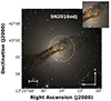 |
Fig. 1. Colored image of Centaurus A (NGC 5128) constructed from RGB images obtained with the Swope telescope located at the Las Campanas Observatory. SN 2016adj occurred within the central dust lane, just southeast of a very bright, and typically saturated foreground star. |
Given the proximity to Earth, SN 2016adj offers an excellent opportunity to study a SE SN in a significantly dusty environment and the conditions associated with the formation of carbon-monoxide (CO) molecules. Before delving into our analysis, we provide information on SN 2016adj’s story of discovery and the community’s earlier efforts in determining its spectral classification.
SN 2016adj was discovered on 2016 February 08.56 UT (i.e., JD-2457427.06) by the Backyard Observatory Supernova Search (BOSS; Marples et al. 2016) at an apparent V-band magnitude of 14.0 mag. As previously mentioned, SN 2016adj occurred in Centaurus A with (J2000.0) coordinates of  and Dec = −43° 00′57
 96 (Kelly et al. 2016). An inspection of Fig. 1 revealed that SN 2016adj is located (on the sky) in close proximity to a bright foreground star.
Kiyota et al. (2016) reported on 2016 February 08.69 UT multicolor photometry of SN 2016adj suggesting the light emitted by SN 2016adj suffered significant reddening. An inspection of a low signal-to-noise optical spectrum of SN 2016adj, obtained with the Lijiang 2.4-m telescope on 2016 February 08.9 UT, led Yi et al. (2016) to initially report a tentative hydrogen-rich SN II classification. A spectrum taken several hours later (2016 February 09.2 UT) at the Las Campanas Observatory (LCO) led to the first indication of SN 2016adj of being a stripped envelope SN Ib (Stritzinger et al. 2016). Soon after, Hounsell et al. (2016) and Thomas et al. (2016) both proposed a SN IIb classification. From our detailed study of the optical and near-infrared (NIR) spectra presented in Sect. 3, and following the standard SN classification taxonomy, we demonstrate that SN 2016adj is in fact a carbon-rich SN Ic.
Distance to Centaurus A. Centaurus A was discovered by James Dunlop in the 1820s and is the fifth brightest galaxy in the night sky. To date, Centaurus A has served as a laboratory to study black-hole accretion physics, determine AGN feedback effects, and understand spectacular X-ray and radio jets (see Israel 1998, for a review). The Hubble type of Centaurus A is widely debated with different camps of thought favoring either an S0p or E0p Hubble type, however, as discussed by Harris (2010), there are indications from its halo and individual stars it is more akin to an Ep galaxy.
To date Centaurus A has hosted the peculiar type Ia SN 1986G, which was also located within the central dust lane, southeast from the center. Given the discovery of these two SNe within the central region of Centaurus A strongly suggests it experienced merger activity which generated a burst of star formation (see, e.g., Della Valle & Panagia 2003). The observed colors of SN 1986G suggest significant host-galaxy reddening, which Phillips et al. (1987) characterized with a host-galaxy color excess of E(B − V)host ∼ 0.7 mag (see also Ashall et al. 2016), while polarimetry studies suggest a total-to-selective absorption coefficient of  (Hough et al. 1987; Patat et al. 2015). As shown in Sect. 4, we infer host-galaxy reddening parameters along the line-of-sight to SN 2016adj of
  and
and  mag.
mag.
The NASA Extragalactic Database (NED)1 provides a heliocentric red-shift z = 0.00183 ± 0.00002 and a red-shift velocity of 547 ± 5 km s−1 (Fouque et al. 1992). NED provides a number of direct distance measurements included the Cepheid distance d = 3.42 ± 0.18 (random) ±0.25 (systematic) Mpc (Ferrarese et al. 2007), or a distance modulus μ = 27.67 ± 0.12 (random) ±0.16 (systematic) mag, which is adopted throughout our analysis to set the absolute flux scale.
The structure of this paper is as follows. Brief properties of our data set are presented in Sect. 2, followed by our analysis of the spectroscopic and photometric evolution in Sects. 3 and 4, respectively. Rough estimates of key explosion parameters are estimated in Sect. 5, while in Sect. 6 pre-explosion images are examined to place loose constraints on the progenitor star. Next in Sect. 7 our results of modeling the CO first overtone feature are presented, followed by Sect. 8 dedicated to the emergence of hydrogen features in the post maximum near-IR spectra of SN 2016adj as well as a discussion on the increasing incidences of hydrogen features appearing in other SNe Ic which interact with H-rich circumstellar material. The manuscript ends with our conclusions in Sect. 9, which is then followed by four appendices including a number of complementary figures based on the analysis of both our unpublished and published data.
2. Data acquisition and reduction
We present an extensive ground-based set of observations of SN 2016adj, complemented with some public ultraviolet (UV) observations. More complete details on the various facilities, the data obtained, and the reduction techniques applied are provided in Appendix A.
In short, the bulk of the ground-based optical and NIR photometry and spectroscopy were taken by Carnegie Supernova Project-II (Phillips et al. 2019, hereafter CSP-II) and the Public ESO Spectroscopic Survey of Transient Objects (Smartt et al. 2015, hereafter PESSTO). Finally, the earliest optical image was fortuitously obtained with the ESO-Paranal VST (VST Survey Telescope) ∼20 days prior to maximum light.
Turning to space-based data, a measurement of the pre-maximum ultraviolet (UV) flux is obtained from single channel images obtained with the UVOT camera on board the Neil Gehrels Swift Observatory (Gehrels et al. 2004).
3. Spectroscopy
3.1. Optical
Sixteen optical spectra of SN 2016adj are plotted in Fig. 2 covering 14 epochs between −7 days to +156 days2. A journal of all spectroscopic observations of SN 2016adj is provided in Table 1. As previously noted by the initial classification reports and clearly apparent in Fig. 2, the blue end of the optical spectra suffers prevalent suppression in flux due to significant host reddening. Additional signatures of high host reddening take the forms of the conspicuous Na I D λλ5890, 5896 doublet feature, and as well with the 5780 Å diffuse interstellar band (DIB) line resolved in the +2.4 days spectrum obtained with the Magellan telescope equipped with the medium resolution spectrograph MagE. The Na I D features along with other prominent features in the spectra of SN 2016adj are marked with vertical lines and labeled in Fig. 2, while Table 2 summarizes the ions attributed to the various spectral features identified in the optical time series.
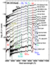 |
Fig. 2. Optical spectra of SN 2016adj from −7 days to +156 days. Phase and telescope facility are indicated on the right of each spectrum. Prevalent spectral features are marked with vertical dashed lines and labeled. Telluric absorption features are labeled with Earth symbols, while for the +43 days to +49 days spectra possible over-subtraction of host-galaxy Hα emission is masked by a translucent black region (see Appendix A.2 for details). |
Journal of spectroscopic observations.
Spectral line IDs in the optical.
The earliest optical spectra are relatively featureless exhibiting only a handful of notches, however by a week past maximum, a number of prominent P Cygni features do emerge. Specifically, the Ca II NIR triplet and the nearby O Iλ7774 lines are observed from the first epochs with ever-increasing pEW values. At the blue end of the spectra extended below 4000 Å, narrow Ca II H&K features are also identified around maximum light. Between −7 days to +8 days the spectra also exhibit a feature around 6500 Å, which the classification reports mentioned in Sect. 1 largely attribute to Hα and hence the initial SN Ib/IIb classification of SN 2016adj. If this classification were correct then He I features are expected to be present. However the maximum phase optical spectra do not exhibit any evidence of such features. Moreover, He I features do not emerge in any of the post maximum spectra when such features are known to emerge in SNe IIb/Ib (see Holmbo et al. 2023, and references therein). As an alternative, we suggest the 6500 Å feature is formed by C IIλ6580 (e.g., Valenti et al. 2008). Furthermore, an absorption feature around ∼7100 Å could be produced by C IIλ7234. In support of these C II associations are at least ten individual C I features identified in the NIR spectra of SN 2016adj (see below).
Scrutiny of the last two spectra obtained on +116 days and +156 days of SN 2016adj in Fig. 2 reveals the emergence of forbidden [O I] λλ6300, 6363 and [Ca II] λλ7291, 7324 lines, as well as narrow emission lines of Hβ and Hα. The Balmer lines are characterized by a full-width-half-maximum velocity (vFWHM) of a few 100 km s−1, and are attributed to an underlying H II region.
Figure 3 shows the time evolution of the Doppler velocity at maximum absorption (−vabs) inferred from the early C IIλ6580 and C IIλ7234 features, the Fe IIλλ5018, 5169 features, the Sc IIλλ5531, 5663, 6246 features, as well as the C Iλ9086, C Iλ10695, C Iλ11330 and C Iλ12615 features. While Sc is often seen in SNe II (arising from primordial material in the H envelope), similar Sc II lines have recently been detected in the superluminous type Ic SN 2020wnt (Gutiérrez et al. 2022) and the type Ic SN 2021krf (Ravi et al. 2023).
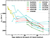 |
Fig. 3. Measurements of −vabs for a handful of mostly prominent features (see legend) in the optical and NIR spectra of SN 2016adj, plotted vs. days relative to the epoch of the B-band maximum. |
The ejecta velocity values inferred from SN 2016adj are on the low side of mean SNe Ic values from literature samples, however, they are not unprecedented. For example, similar low ejecta velocities have been inferred in a handful of other SNe Ic including SNe 2004gt, 2007hn, 2009dt, 2011dm, and 2021kfr (e.g., Valenti et al. 2016; Taddia et al. 2018a; Holmbo et al. 2023; Ravi et al. 2023). One should also keep in mind that SNe Ic exhibit a range of rise times, and therefore one must approach with caution comparisons of ejecta velocity measurements of objects scaled in phase with respect to peak brightness rather than explosion epoch. Nevertheless, the low ejecta velocity of SN 2016adj hints at it having a low explosion energy, a high ejecta mass, or a combination of the two (see below).
3.2. NIR Spectroscopy: Early C I and post-maximum H I features
Our NIR time series offers a rare chance to view in detail the evolution of this wavelength region of a SN Ic over a six month period. The NIR spectral time series of SN 2016adj plotted in Fig. 4 extends from +0 days to +176 days. Prominent features in the spectra are indicated with vertical lines and labeled. A summary of these features are provided in Table 3, and include the Ca II triplet, ten conspicuous C I features, two subtle O Iλ9263 and O Iλ11 287 features, and the Mg Iλ15 025 and Mg Iλ21465 features. The −vabs values of four of these C I features are plotted in Fig. 3 along with the values inferred from the various optical lines. The velocity of these C I features are in good agreement with those inferred from the C II features present in the early optical spectra.
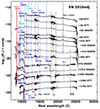 |
Fig. 4. NIR spectral time series of SN 2016adj covering 6 months of evolution beginning from the epoch of the B-band maximum. The phase and telescope are indicated to the right of the spectra. The locations of various spectral features are identified with vertical dashed lines and labeled. The lines indicate the spectra where the features are identified. Telluric regions were labeled with an Earth symbol. |
Spectral line IDs in the NIR.
Banerjee et al. (2018) presented a NIR time series of SN 2016adj from −5 days to +61 days, and in their analysis preferred a SN IIb classification. Contrary to Banerjee et al. (2018), we do not identify from the onset of observations hydrogen features associated with Pa-δ (Pa-7) λ10 049, Pa-γλ10 938, Pa-βλ12 822, and Br-γλ21 661. Furthermore, we do not find features attributable to Pa-δ and Pa-βλ12 822. A feature around ∼21 500 Å is more likely Mg Iλ21 465 rather than Br-γλ21 661. There is a notch in the early spectra that could be Pa-γλ10 938, but the identification is not conclusive. Banerjee et al. (2018) also suggest a feature around ∼9230 Å that might be produced by a blend of Pa-ζ (Pa-9) λ9232 and Mg Iλ9258 blend, however, based on the location and time evolution of the feature, we suggest a O Iλ9263 identification. We note that the NIR time series shows no evidence of Pa-αλ18751 at any time; however, Pa-α must be very strong to see the signal through the telluric haze (see, e.g., Shahbandeh et al. 2022).
Interestingly, by +58 days (corresponding to the last epoch spectrum presented by Banerjee et al.) we identify the emergence of a handful of hydrogen features. Among our time series these features are best revealed in the medium-resolution echelle spectrum obtained on +97 days. Plotted in the top panel of Fig. 5 is the +116 days optical spectrum with the two narrow Balmer emission features marked and labeled, while the middle panel displays the +97 days spectrum containing hydrogen features attributed to: Pa-δ, Pa-γ, Pa-β, Br-ζ, and Br-γ. The seven hydrogen features contained within the top two panels are also plotted in velocity space within the bottom row of Fig. 5. The optical spectrum reveals narrow Hβ and Hα emission with vFWHM∼ a few ×100 km s−1. Inspection of the features (see also Fig. 2) seem to tentatively suggest a broader component for both features, however, this is speculative due to the poor signal-to-noise of the data. In the optical data the narrow component is likely due to nebular emission lines associated with an underlying H II region (see Appendix B). Turning to the NIR Paschen lines, they exhibit P Cygni profiles with −vabs ∼ 1500 − 2500 km s−1.3 The wavelength regions containing the Bracket lines are of lower signal-to-noise, but they also exhibit emission features with vFWHM ∼ 1000 km s−1 with some line structure.
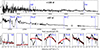 |
Fig. 5. Potential signatures of an interaction with circumstellar hydrogen. Top: Low-resolution optical- +116 days and middle: echelle NIR +97 days spectra of SN 2016adj. The optical and NIR spectra have been color-corrected to match coeval broad-band photometry. Both spectra are de-reddened using the reddening parameters estimated in Sect. 4.2. The positions of conspicuous hydrogen features are marked with vertical lines and labeled. Bottom: Zoom in velocity space of the Balmer, Paschen and Bracket series features. The Paschen features exhibit P Cygni profiles with −vabs values ∼1500 − 3000 km s−1 and vFWHM ∼ 1000 km s−1. The red lines correspond to pseudo-continuum fits determined by Monte Carlo simulations. We note that the flux of the nebular [N II] λλ6548,6584 lines on either side of Hα is not included in its emission-line flux measurement. |
We next measure the emission and absorption line flux values associated with the H features in the two spectra shown in Fig. 5. To do so, a blue and red edge for the features is first defined by applying an iterative second order polynomial fit, which enables the pseudo-continuum associated with the features to be defined. Emission and absorption flux values are then estimated by integration of the flux contained within the area defined by the emission and absorption components and the pseudo-continuum. This process is applied following a Monte Carlo approach consisting of 100 realizations, which provide an estimate on the uncertainty of the estimated flux values. The MC realizations are over-plotted with the features shown in the bottom panels of Fig. 5, and the emission and absorption flux values are summarized in Table 4. In Sect. 8 the emission-line flux values are used as a diagnostic to estimate the density of the line forming region.
3.3. SN 2016adj is a type Ic supernova
Banerjee et al. (2018) alluded to the possibility that SN 2016adj could be a hydrogen- and helium-deficient SNe Ic, but due to a lack of optical spectra and interpretation of the NIR spectra that is contrary to our own, they preferred a SNe IIb classification. Based on the detailed comparisons to other SE SNe, we find SN 2016adj is a SN Ic. Here the optical and NIR spectra of SN 2016adj are compared to similar epoch observations of the various SE SN subtypes in order to support our reclassification of SN 2016adj4.
First, Fig. 6 compares the −3 days, +5 days and +26 days optical spectra of SN 2016adj to similar phase spectra of the type IIb SN 2011dh (Ergon et al. 2014), the type Ib SN 2007Y (Stritzinger et al. 2009), and the type Ic SN 2005az (Bianco et al. 2014). These objects were chosen as they are excellent representatives of their SE SN subtype and have similar phase spectra as SN 2016adj. The spectra of SN 2005az are found to be very similar to those of SN 2016adj. Both objects clearly lack the Balmer features that are quite prevalent in SN 2011dh. Moreover, SN 2005az and SN 2016adj do not exhibit over their evolution He I lines which are so apparent in the post-maximum spectra of SN 2007Y and SN 2011dh. From this comparison alone, we find that SN 2016adj is fully consistent with being a SN Ic.
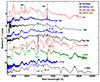 |
Fig. 6. Selection of optical spectra of SN 2016adj de-reddened and compared with similar phase spectra of the type IIb SN 2011dh (Ergon et al. 2014), the type Ib SN 2007Y (Stritzinger et al. 2009), and the type Ic SN 2005az (Bianco et al. 2014; Modjaz et al. 2014). The epochs labeled next to each spectra are relative to the epoch of r-band maximum. Similar to the type Ic SN 2005az, the spectra of SN 2016adj lack Balmer lines (dashed magenta) and He I features (red dash lines), both of which develop past maximum in the SNe 2007Y and 2011dh. C II lines are indicated with blue dashed lines. |
Turning to longer wavelengths, Fig. 7 compares the +32 days NIR spectrum of SN 2016adj with the ≈+15 days spectrum of the type Ic SN 2007gr (Valenti et al. 2008), the +16 days spectrum of SN 2011dh (Ergon et al. 2014), and a SYNOW synthetic spectrum for solely C I (Millard et al. 1999). The spectra of SN 2007gr and SN 2016adj are nearly identical, exhibiting the same features including, most notably, the C I lines. As compared to SN 2011dh, both objects lack the prominent He Iλ20581 line. Within this context, the strong 10 500 Å feature in SN 2007gr and SN 2016adj is attributed to C Iλ10 695 as is supported by the comparison with the SYNOW spectrum. In the case of SN 2011dh, its 10 500 Å feature is then attributed to He Iλ10 831 with a possible contribution from C Iλ10 695. Based on these findings, the NIR spectra of SN 2016adj are in full agreement with it being a SN Ic.
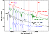 |
Fig. 7. De-reddened NIR spectrum of SN 2016adj taken at +32 days compared with a +15 days spectrum of the type Ic SN 2007gr (Valenti et al. 2008), a +16 days spectrum of the type IIb SN 2011dh (Ergon et al. 2014), and the SYNOW synthetic spectrum computed for C I (Millard et al. 1999). Prevalent C I lines, as for example the strong feature around 11 000 Å, are present in the NIR spectrum of SN 2016adj. As in the optical, no traces of He I are identified in the longer wavelength spectrum of SN 2016adj. This is contrary to the He I features in the spectrum of SN 2011dh, particularly the prevalent P Cygni feature at 20 581 Å. |
3.4. Detection of the first CO overtone
CO emission was first identified in SN 2016adj by Banerjee et al. (2016), who noted the presence of the first CO overtone (2–0) band head (2.25 − 2.45 μm) in a spectrum obtained at +52.6 days. The same authors confirmed this initial assessment with a spectrum obtained at +58.7 days (Banerjee et al. 2018). Turning to our NIR spectroscopic time series extending through +176 days (see Fig. 4), the first CO overtone is found to have emerged already by +41 days. This is ≈10 days earlier than previously reported, and to our knowledge, among the earliest CO signature detected in the wake of a supernova (Banerjee et al. 2018; Ravi et al. 2023).
In Sect. 7 we turn to CO models to estimate key physical parameters characterizing the underlying CO emission region.
4. Photometry
4.1. Light curve parameters
Our UV/optical (UVW1, u, B, g, V, r, i) and NIR (Y, J, H, K) light curves of SN 2016adj are shown in Fig. 8. The bulk of the photometry follows the flux evolution beginning a few days prior to the epoch of B-band maximum through ≈+70 days in the optical and ≈+210 days in the NIR. In addition, a very early (−19.7 days) i-band photometric measurement was computed from a serendipitous image obtained by the VST.
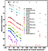 |
Fig. 8. Optical and NIR photometry of SN 2016adj plotted relative to the epoch of the B-band maximum from observations obtained by CSP-II, PESSTO, with the ESO-Paranal VLT Survey Telescope (VST) equipped with OmegaCAM, and with the UVOT camera on board Swift. To facilitate the comparison of photometry obtained with different instruments, in some cases offsets have been applied as indicated in the legend. A low-order polynomial function is overplotted on each light curve and used to infer the time and value of peak. Epochs of spectroscopic observations are indicated by black (visual) and red (NIR) segments. |
The light curves of SN 2016adj in the bluer bands are much fainter than the light curves of the redder bands. This is a result of the significant host-galaxy reddening affecting the light of SN 2016adj. Indeed, the K-band photometry is ≈6 magnitudes brighter than the V-band photometry, suggesting a host-galaxy visual extinction of the same order. An indication of significant extinction is also evident from the comparison between the observed colors of SN 2016adj with those of SE SNe intrinsic color-curve templates (see below).
Comparison among the light curves indicates that the bluer bands decline faster than the redder bands. This is typical of the evolution documented in both SNe II and SE SNe samples (e.g., Taddia et al. 2015, 2018b; Valenti et al. 2016; Hicken et al. 2017; de Jaeger et al. 2019). The epoch and apparent magnitude at peak for each light curve was determined through the use of low order polynomial fits, as well as the light-curve decline rate parameter Δm15 (Phillips 1993). The values of these light curve parameters and the absolute peak magnitudes (see below) are summarized in Table 5.
Light curve parameters.
4.2. Reddening of SN 2016adj
According to Schlafly & Finkbeiner (2011) and reported by NED, the Milky Way reddening in the direction of Centaurus A is non-negligible with a color excess of E(B − V)MW = 0.1 mag, which upon adopting the standard Milky Way total-to-selective absorption coefficient, RV = 3.1, corresponds to the Milky Way visual extinction value  mag. Located within the central dust lane of Centaurus A, it is not surprising that SN 2016adj suffers significant host-galaxy reddening. This is manifested in the significant suppression of flux on the blue end of the optical spectra (see Fig. 2) and the presence of conspicuous and saturated Na I D features.
Determining an accurate estimate of the host reddening of SN 2016adj is a challenging task. As a first step the equivalent width (EW) of the DIB 5780 Å feature measured from our MagE spectrum implies, following Eq. (6) of Phillips et al. (2013), an  mag. Assuming an RV ∼ 3.1 this corresponds to E(B − V)host ∼ 1.0 mag.
Turning to pre-explosion (February 2015) integrated field spectroscopy observations obtained with the VLT (+MUSE; see Appendix B) and assuming a canonical Hα/Hβ intrinsic ratio of 2.86, the Balmer decrement implies a gas-phase color excess at the location of SN 2016adj of E(B − V)gas = 0.92 ± 0.37 mag.
We next estimated the host reddening by comparing the observed colors of SN 2016adj to the intrinsic SE SN color-curve templates presented by Stritzinger et al. (2018). Plotted in Fig. 9 are the (X − V, where X = u, B, g, r, i, Y, J, H colors) of SN 2016adj corrected for Milky Way reddening and the SN Ic color-curve templates. Taking the mean difference between the Milky Way reddening-corrected colors and the color-curve templates for each color combination, yields the E(V − X)host values plotted as a function of the effective filter wavelength in Fig. 10. Overplotted to these values are three different best-fit reddening laws representing the Fitzpatrick (1999, hereafter FTZ99) reddening law with  and
and  = 5.7 ± 0.7 mag (reduced χ2 = 20.7), the Goobar (2008, G08) power-law model (reduced χ2 = 11.5), and the FTZ99 law with
  set as a free parameter (reduced χ2 = 5.6). Given the reduced χ2 values we adopt in our analysis the host reddening parameters of
  = 5.7 ± 0.7 and
  = 6.3 ± 0.2 mag (i.e., E(B − V)host = 1.1 mag), which is consistent with the reddening estimated from Balmer decrement measurements computed using a MUSE spectrum.
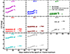 |
Fig. 9. Optical and optical/NIR colors of SN 2016adj corrected for Milky Way reddening (filled symbols) vs. days relative to the time of the V-band maximum. The solid lines correspond to the SN Ic intrinsic color-curve templates presented by Stritzinger et al. (2018), while the unfilled symbols correspond to the fit of the templates to the filled symbols. The E(V − H)host color excess suggests an |

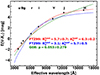 |
Fig. 10. Optical and NIR E(V − X)host (where X = u, B, g, r, i, Y, J, H) color excess measurements of SN 2016adj, plotted as a function of the effective wavelength of passband X. Each color excess measurement represents the difference between the observed color (corrected for E(B − V)MW) and the intrinsic color-curve template for SN Ic shown in Fig. 9. The red dashed line corresponds to the best Fitzpatrick (1999) reddening law model fit characterized by a ratio of total-to-selective absorption |


To assess the validity of the FTZ99 model characterized by a high  value, we turn to Fig. 11 which presents a comparison between an intrinsic SN Ic template spectrum at maximum (Holmbo et al. 2023) and SN 2016adj at −1.6 days. The spectrum of SN 2016adj is shown corrected for the two sets of reddening parameters, that is,
  = 3.1 and
  = 5.7 mag, and
  = 5.7 and
  = 6.3 mag. Clearly the spectrum of SN 2016adj corrected for the higher reddening parameters provides a much better match to the shape of the template spectrum. This gives an additional measure of confidence that the reddening values inferred with a higher
  value more accurately describe the reddening of this system.
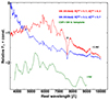 |
Fig. 11. Comparison of the −1.6 days spectrum of SN 2016adj de-reddened for Milky Way reddening and also assuming the two different sets of reddening parameters discussed in Sect. 4.2 and indicated in the plot. Also plotted in green is the CSP-I SN Ic spectral template at +0 days (Holmbo et al. 2023). |
A high  value as inferred for SN 2016adj is not without precedent. For example, RV values on the level of 4–6 have been inferred from observations of the Ophiuchus and Taurus molecular clouds (e.g., Mathis 1990). Moreover, Stritzinger et al. (2018) demonstrated that SNe Ic are more likely to occur in environments characterized by larger
  values compared to SNe IIb/Ib, while high values of RV are expected as SNe Ic are preferentially associated with regions of on-going star formation (Anderson et al. 2015; Galbany et al. 2017; Sextl et al. 2023).
4.3. Absolute magnitude light curves of SN 2016adj
With reddening parameters and distance in hand, the absolute magnitude light curves of SN 2016adj are readily computed as shown in Fig. 12. To demonstrate the effects of host-reddening, absolute magnitudes are plotted with (empty circles) and without (filled circles) host-reddening correction. Also shown in the figure are the canonical SE SN light curves from Taddia et al. (2018b), scaled to match the average SN Ic peak absolute magnitudes and shifted to match the average time differences between the epochs of maximum in the different filters. Clearly, the absolute light curves of SN 2016adj corrected for host reddening provide a much better match to the template light curves. Also plotted in Fig. 12 are the light curves of the type Ic SN 2005az (Bianco et al. 2014), which is spectroscopically similar to SN 2016adj.
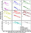 |
Fig. 12. Absolute magnitude light curves of SN 2016adj compared to the CSP-I SE SN template light curve scaled in time and to the average peak absolute magnitude determined from the CSP-I SN Ic sample. The light curves of SN 2016adj are plotted with and without host-extinction correction as indicated in the legend. The prevalent reddening is visible in the bluer bands with the Milky Way reddening corrected light curves of SN 2016adj being much fainter compared with the average SN Ic light curves. Also shown for comparison are the light curves of the type Ic SN 2005az (Bianco et al. 2014) which, as demonstrated in Fig. 6, is spectroscopically similar to SN 2016adj. The error bars accompanying the magnitudes of SN 2016adj account for the uncertainties in the distance and the reddening parameters |


The extinction-corrected light curves of SN 2016adj suggest it reached an absolute peak B-band magnitude MB ∼ −18.0 ± 0.1, which is approximately a magnitude more luminous than the “average” SN Ic. The peak absolute magnitudes for the entire sequence of light curves computed with and without host-extinction corrections are listed in Table 5. Inspection of the other bands red-ward of the B band reveals peak values between ∼ − 18.5 to −19.1 mag.
5. Bolometric properties and explosion parameters
5.1. Pseudo-bolometric light curves and peak luminosity
Here we describe the techniques used to construct the pseudo-bolometric light curves of SN 2016adj which are used to estimate key explosion parameters based on semi-analytical models appropriate for SE SNe (e.g., Arnett 1982; Khatami & Kasen 2019).
First, the broad-band optical and NIR photometry of SN 2016adj was linearly interpolated in time and corrected for reddening. The resulting magnitudes were converted to their respective AB magnitude values using the terms provided in Table 16 of Krisciunas et al. (2017) and then converted to monochromatic fluxes. These flux points ranging over optical to NIR wavelengths enable us to construct spectral energy distributions (SEDs) of SN 2016adj for each epoch of observations and are corrected for the dust reddening using the FTZ99 reddening law characterized by  = 5.7
= 5.7  = 6.3 mag (see Sect. 4.2).
With SEDs extending from the u to the Ks bands in hand, black body (BB) functions were fit to each SED enabling estimates of the BB temperature (TBB) and the BB radius (RBB) of the underlying emission region. The results of this procedure are plotted in Fig. 13 with the TBB and RBB profiles plotted in the middle and bottom panels, respectively. The inferred BB parameters reveal a maximum RBB of about 4 × 1015 cm and TBB values decreasing over time from 6000 K to 5000 K5.
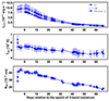 |
Fig. 13. Bolometric light curves (top), black-body temperature profile (middle), and black-body radius profile (bottom) of SN 2016adj. Using broadband photometry corrected for both Milky Way and host-galaxy reddening, bolometric light curves were computed by: (i) integrating the best-fit Planck function to the SEDs (dashed line denoted by LBB), (ii) trapezoidal integration of the SEDs (filled squares denoted by L∫) and (iii) through the combination of the g- and i-band photometry combined with the bolometric corrections presented by Lyman et al. (2014, filled circles denoted LBC, Lyman). We adopted our best host-reddening estimate, that is, a FTZ99 reddening law with |


The pseudo-bolometric luminosity of SN 2016adj was computed following three methods. In the first method each SED was summed over wavelength using trapezoidal integration to obtain the UltaViolet-Optical-nIR (UVOIR) flux (FUVOIR), which was multiplied with 4πD2 to produce the UVOIR luminosity (LUVOIR). In the second method, the best-fit BB Planck functions were integrated and multiplied by 4πD2 to obtain LBB, and in the third approach the g- and i-band photometry was combined with the bolometric corrections presented by Lyman et al. (2014). The resulting pseudo-bolometric light curves constructed following these methods are plotted in the top panel of Fig. 13, while the middle and bottom panel display the temporal evolution of TBB and RBB, respectively.
The pseudo-bolometric light curve computed using the Lyman et al. (2014) corrections indicates the SN reached a peak luminosity ∼9.5 ± 1.5 × 1042 erg s−1. Here the uncertainty accounts for the error in the adopted distance translating to about 12% uncertainty in luminosity. An additional 16% systematic error should be added due to the reddening uncertainty. The pseudo-bolometric light curve computed with the simple integration of the SEDs starts at around maximum when all the bands are covered, and it is obviously fainter than the other two bolometric light curves which include extrapolation corrections for wavelengths not covered by the observed passbands. The pseudo-bolometric light curve computed via BB integration is slightly brighter than the one obtained with the Lyman et al. bolometric corrections, as it tends to overestimate the flux in the UV which does not follow the emission of a BB function.
5.2. Explosion epoch
An estimate of the explosion epoch of SN 2016adj is needed before we can accurately fit its bolometric light curve with semi-analytical models. In Fig. 14 the i-band light curve of SN 2016adj (in flux units) is plotted along with that of the SDSS-II SN Ibc template i-band light curve (Taddia et al. 2015); scaled and shifted to match the peak of SN 2016adj. The template reproduces the light curve shape quite well without the need to use a light-curve stretch parameter.
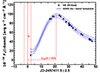 |
Fig. 14. Observed i-band photometry of SN 2016adj in flux units (black symbols) vs. days relative to the estimated explosion epoch (JD–2457411.5 ± 2.5). Overplotted as a blue solid line is the SN Ib/c i-band template light curve presented by Taddia et al. (2015), scaled and shifted to match the light curve of SN 2016adj. The blue dashed lines corresponds to a 1-σ uncertainty error snake. The epoch of the inferred explosion time, t0, is indicated by the vertical red solid line and assumes an i-band rise time of 21 days (see Taddia et al. 2015). The time difference between the inferred explosion date and the first i-band epoch is 2.5 days, which corresponds to the uncertainty of our estimated rise time. |
If we assume that the template peak corresponds to the peak of the observed i-band light-curve of SN 2016adj on JD-2457432.5 ± 2.5, we infer an explosion epoch of JD-2457411.5 ± 2.5. The quoted uncertainty corresponds to the difference between the derived explosion epoch and the first i-band detection of SN 2016adj. The difference between our inferred explosion epoch and the epoch of i-band maximum indicates a rise time of 21.0 ± 2.5 days. This value is about a week longer than the average rise time value inferred from an analysis by Taddia et al. (2015) of the SDSS-II SN Ic and SNe Ic-BL samples, and more aligned with the average rise-time values inferred from their SN IIb and SN Ib samples. However, longer SNe Ic rise times are not without precedent, for example, SN 2007ms (≈22 days, Prentice et al. 2016), SN 2011bm (≈40 days, Valenti et al. 2012), iPTF11jgj (≈21 days, Prentice et al. 2016; Barbarino et al. 2021), and SN 2021krf (≈24 days, Ravi et al. 2023) exhibited rise times in excess of 20 days.
5.3. Explosion parameters via Arnett’s model
With the epoch of explosion in hand, the pseudo-bolometric light curve constructed using the Lyman et al. (2014) bolometric correction is plotted in Fig. 15, along with our best-fit Arnett (1982) model. Following the procedure adopted by Taddia et al. (2018b), the Arnett model was fit to the luminosity measurements extending to 40 days past explosion which in the case of SN 2016adj is 61 days past explosion. At this phase the ejecta is still optically thick to the gamma-ray photons produced from the 56Co to 56Fe decay chain. The model assumes the ejecta has a constant density and a constant opacity of 0.07 cm2 g−1 (see Taddia et al. 2018b), and the velocity of the bulk of the ejecta at maximum is 6500 ± 2500 km s−1, as inferred from the optical C II and C I features (see Fig. 3).
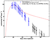 |
Fig. 15. Pseudo-bolometric light curve of SN 2016adj constructed with the bolometric corrections from Lyman et al. (2014) and plotted along with our best-fit Arnett (1982) model. The model was fit to the luminosity measurements shown in blue and consisting of epochs extending up to 61 days post explosion when the ejecta remains to be optically thick to the gamma-rays emitted by radioactive decay (see Taddia et al. 2018b, and references therein). |
The pseudo-bolometric light curve of SN 2016adj and the best-fit Arnett model are plotted Fig. 15. The model fit corresponds to an ejecta mass  , an explosion kinetic energy
  erg s−1, and a 56Ni mass
  . Here the uncertainties account for the errors on the ejecta velocity and the inferred explosion epoch. The ejecta velocity error dominates the uncertainties on EK and Mej, while the explosion epoch error mainly contributes to the 56Ni estimate. In addition to these uncertainties, we add an error of ±0.1 M⊙ to Mej to account for the fitting error, which is negligible to the EK and 56Ni estimates. Furthermore, related to the uncertainties in the adopted distance (12%), the reddening parameters (16%), and possible (10%) contamination from an underlying light echo (see Stritzinger et al. 2022), we tack onto the 56Ni uncertainty value ±0.06 M⊙, ±0.08 M⊙, and ±0.05 M⊙, respectively. We also considered the affect of the temporal range of the data used to compute the best-fit Arnett model. Changing the fitting restriction from 61 days post explosion by ±20 days results in explosion parameter estimates of Mej, EK and the 56Ni mass that differ by the modest levels of ±11%, ±8%, and ±4%, respectively.
Inspection of Fig. 15 reveals that the best-fit model significantly diverges from the bolometric light curve beginning around +40 days past explosion. This could be indicative of an additional energy source beyond 56Ni decay and light echo emission, which would then contribute to the high peak luminosity of SN 2016adj. Additional energy sources considered in previous SE SNe studies include CSI, or emission magnetic dipole radiation emitted by a proto-neutron star in the form of a either a magnetar or millisecond pulsar (e.g., Kasen & Bildsten 2010; Ravi et al. 2023). In context with SN 2016adj, spectroscopic signatures of CSI only appear well after maximum light making this not a very viable possibility (see Sect. 8), while magnetar emission models tend to produce SNe with longer rise times, high peak luminosities, and broad light curves (e.g., Kasen & Bildsten 2010; Taddia et al. 2018a; Gutiérrez et al. 2021; Omand & Sarin 2024).
With the caveats related to the high uncertainty in the peak pseudo-bolometric luminosity of SN 2016adj and that the basis of Arnett’s Rule relies on a number of assumptions in mind, we briefly compare our results for SN 2016adj to those in the literature. Barbarino et al. (2021, see their Table 7) compares average explosion parameters estimates of the iPTF SN Ic sample to those found by other authors who consider various size SN Ic samples (Drout et al. 2011; Lyman et al. 2016; Prentice et al. 2016, 2019; Taddia et al. 2018b). In general, the explosion parameters computed for SN 2016adj are not radically different than the average values listed by Barbarino et al. (2021). The EK and Mej estimates are within the range of the average values found by most of the other works, while the 56Ni mass of 0.5 M⊙ is a factor of two more than the typically average value of 0.25 M⊙. Though it is worth mentioning the SN Ic sample of Barbarino et al. (2021) contained a number of objects with 56Ni masses of ∼0.5 M⊙ (see also Sollerman et al. 2022, for a similar analysis using a Zwicky Transient Factory SE SNe sample).
When considering all of the uncertainties, the minimum of the 56Ni mass confidence interval of ≈0.3 M⊙ is relatively high compared to the typical sample median values (see Table 9 in Taddia et al. 2018b). However, 56Ni masses in excess of 0.3 M⊙ for SNe Ic are not without precedent. Anderson (2019) presented a meta-analysis regarding 56Ni mass estimates for both hydrogen-rich and SE SNe, finding a median SN Ic 56Ni mass of  , with a handful of objects, for example, PTF 12gzk (Prentice et al. 2016), iPTF15dtg (Taddia et al. 2016), and SN 2011bm (Valenti et al. 2012; Lyman et al. 2016; Prentice et al. 2016) with values exceeding 0.3 M⊙. We conclude here by pointing out that within standard core-collapse SNe simulations it is difficult to produce ≳0.2 M⊙ of 56Ni (see, e.g., Müller 2016; Sollerman et al. 2022, and references therein), implying values inferred from Arnett’s model are overestimated and/or objects with high 56Ni estimates have an additional energy source contributing to their bolometric emission.
6. Progenitor analysis using pre-explosion imaging
We searched the ESO and HST archives for pre-explosion images of Centaurus A containing the position of SN 2016adj. A full summary of the analysis is presented in Appendix C. In short, no source is detected at the position of SN 2016adj in a series of HST (+WFC3; Wide Field Camera 3) and VLT (+NACO; Nasmyth Adaptive Optics System (NAOS); Near-Infrared Imager and Spectrograph (CONICA)) pre-explosion images. Nevertheless, two of the HST images were of high enough quality that limiting magnitudes could be determined, though these do suffer from the uncertainties related to the estimated dust reddening properties. As described in Sect. C.3, we find limiting apparent magnitudes of mF814W > 26.4 mag and mF545M = 25.9 mag. Similarly, the NACO images allow us to place limits of J > 21.6, H > 20.9 and Ks > 21.1 mag on the progenitor. Unfortunately neither the optical limits from HST not the IR limits from NACO allow us to place any meaningful constraint on the progenitor luminosity. The vast majority of known WR stars are fainter than −5.7 in F814W (Eldridge et al. 2013), while the dusty WR stars that are bright in the IR (e.g., Rate & Crowther 2020) would go similarly undetected in our data (K > −7.5).
7. CO emission
7.1. The CO first overtone
The first CO overtone feature in the +41 days NIR spectrum of SN 2016adj is among the earliest detection yet documented in a SN. For comparison, the feature was detected in the type Ic SN 2021krf by +43 days (Ravi et al. 2023), in the type Ic SN 2013ge by +48 days (Drout et al. 2016), while the type Ic SN 2007gr showed signatures of CO by +70 days (Hunter et al. 2009). In addition, in the ∼14 mostly SNe II with CO emission, the CO signature typically emerged months later (Banerjee et al. 2018; Davis et al. 2019).
7.2. CO model fitting
We now turn to comparison of a grid of CO emission models with the first CO overtone feature in the +97 days and +159 days medium-resolution NIR spectra of SN 2016adj. This enables the estimate of key physical parameters of the CO gas including: the temperature (TCO), the velocity (vCO), the ratio of CO+ to CO (aka frac), and a lower limit on the CO mass. First, a grid of CO emission models was computed using a recently developed module contained within the non-LTE HYDrodynamical RAdiation code HYDRA (see Höflich 2003, 2009; Hristov et al. 2021; Hoeflich et al. 2021, and references therein), which enables the determination of the vibrational transition opacities for CO and SiO gas over a range of parameter space.
To determine the best-fit model(s) appropriate for the CO emission in SN 2016adj, a six parameter function was created and used to determine the best-fit. Fitting was performed following a Markov chain Monte Carlo (MCMC) calculation making use of the Python emcee package. The model parameters consist of: (i) an amplitude (A) parameter proportional to the CO mass (MCO), (ii) an underlying continuum fit parameter (b) extending between 22 850 Å to 25 000 Å, (iii) TCO, (iv) vCO, (v) frac, and (vi) a velocity parameter (z). Parameter b takes the functional form of λ−2 and stems from the continuum radiation being formed by free–free emission (Rybicki & Lightman 1979). The z parameter accounts for an arbitrary shift between vCO and the grid of models, although the origin of such velocity offset is unclear. Possibilities include the offset of the progenitors orbital velocity to its host’s systemic velocity, a peculiar velocity of the progenitor within its host, or if the progenitor belongs to a double star system, the binary orbital velocity.
Figure 16 displays the first CO overtone feature in the color-corrected and de-reddened +97 days spectrum of SN 2016adj. Over-plotted is the best-fit MCMC model and the underlying continuum flux extrapolation. For completeness, the MCMC corner plot containing the posterior probability distributions of the model-fit parameters is presented in Fig. D.1. Overall the model agrees well with the data and corresponds to model-fit parameters of A = 1.43 ± 0.12, b = 2.59 ± 0.11 TCO = 3830 ± 170 K, vCO = 2010 ± 270 km s−1, frac = 0.002, z = 0.00145 ± 0.00091. The low inferred value of frac suggests the emission region lacks gamma-rays, non thermal electrons, and/or He+. The underlying CO mass is estimated following: For an optically thin emission region the emissivity per unit mass is given by ηλ = κλ(ρ, v, T)*Bλ(T). Thus the total flux observed will be given by Fλ = MCOηλ/4πD2. Using the fitting results, we find MCO ≈ 2.5 × 10⁻³ M⊙. This value is an upper limit as radiative transfer effects will reduce the emitted luminosity by a factor < 1, however, a non-isothermal emission region could increase the emitted flux.
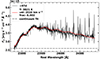 |
Fig. 16. First CO overtone feature in the +97 days NIR medium-resolution spectrum of SN 2016adj (solid black line) compared with the best-fit model (solid red line) characterized by the parameters listed in the legend. The dot-dashed black line corresponds to the underlying continuum flux. |
As previously mentioned, Banerjee et al. (2018) reported on CO emission in SN 2016adj present in their NIR spectral time series. Using a model developed by Das et al. (2009) they estimated from a +64 days spectrum the model parameters: TCO = 4600 ± 400 K, vCO = 3400 ± 150 km s−1, and MCO = 2.1 ± 0.4 × 10⁻⁴ M⊙.
8. Late-time hydrogen features
8.1. Potential signatures of interaction with circumstellar hydrogen
The H features in the post maximum NIR spectra of SN 2016adj with −vabs ≈ 1500 − 3000 km s−1 and vFWHM ∼ 1000 km s−1, coupled with the time scale of their appearance suggests they arise from a narrow decoupling region. The density of the emitting gas can be estimated through the use of line ratios in the classical emission-line nebular case (Osterbrock & Ferland 2006). Using the emission-line flux values determined from the post-maximum spectra presented in Fig. 5 and listed in Table 4, H emission-line ratios are computed relative to Pa-β. The resulting line ratios are listed in Table 6. The inferred line ratios are inconsistent with pure recombination values (i.e., Pγ/Pβ ∼ 0.6) for a gas with a reasonable range of temperature and in pure local thermal equilibrium (LTE). In fact both the Paschen and Bracket line ratios indicate these features are associated with an optically thick gas in non-LTE (NLTE) with electron densities of ne ≳ 1010 − 1011 cm−3 (e.g., Lynch et al. 2000).
Hydrogen emission-line ratios.
Turning to temporal emergence of the H features in the NIR spectra of SN 2016adj, adopting the phase of the spectrum plotted in Fig. 5, photoionization of the shell by the SN shock breakout radiation field, implies a distance (hereafter Ds) between the progenitor and a circumstellar (CS) shell of ∼0.08 pc. However, if the shell was located at this Ds then the H features should have appeared earlier. We therefore assume in the following that the ionization of the shell is caused by CS interaction (hereafter CSI) with the SN ejecta (e.g., Simon & Axford 1966; Chevalier & Fransson 1994). Adopting a velocity for the fastest portion of the SN ejecta to be 25 000 km s−1, CSI implies Ds ∼ 0.007 pc. Adopting a Wolf-Rayet (WR) wind velocity of 1000 km s−1 indicates that the purported shell formed around a decade prior to the supernova.
A confined, optically thick emission region could be associated with a shell located within the CS environment of a WR star (see Crowther 2007, for a review). Often located at or near the center of a complex ring nebula (e.g., Smith 1967), WR stars exhibit significant diversity (e.g., Grosdidier et al. 1998; Marchenko et al. 2010) linked to their robust line-driven winds and other potential mass-loss mechanisms (see Puls et al. 2008).
The morphology and substructures of known WR associated nebula led to the establishment of a classification system (see Chu 1981, and references therein). Firstly, R-type nebula are photoionized H II regions in the nearby vicinity of an WR star. Bona fide associations between WR stars and nebulae include wind-driven W-type WR stars (e.g., Johnson & Hogg 1965; Avedisova 1972; Cappa et al. 2005) and post common envelope evolution E-type WR stars (e.g., Podsiadlowski et al. 2010; Jiménez-Hernández et al. 2020; Schrøder et al. 2020). W-type WR stars exhibit a variety of CS shell(s) and/or wind blown CS bubbles, which can form by a variety of processes.
CS shells may form via wind–wind interaction (e.g., Bransford et al. 1999), for example, putative luminous blue variable (LBV)-like mass ejections (see Smith & Arnett 2014; Vink 2017), or binary interaction with a companion (e.g., Yoon 2017). On the other hand, W-type WR stars associated with colliding-wind binary systems (e.g., WR 140) and pin wheel dust nebulae form a shell from wind-wind interaction between two massive stars during their periastron passage (e.g., Tuthill et al. 2006; Williams et al. 2021). In the case of E-type WR stars such as WR 124 located within the nebula M1-67, its complex 3D structure consisting of bipolar outflows, wind-blown bubbles, and a toroidal structure is aligned with expectations of a binary system that experienced post common envelope evolution (e.g., Chu 1981; Zavala et al. 2022).
The Ds values inferred for a CS shell surrounding SN 2016adj are inconsistent with the order of magnitude higher values reported in the literature for resolved shells produced by wind-wind interaction around WR stars that exhibit Ds values of ≳10 pc (see Bransford et al. 1999, their Tables 1 and 2). In other words, as the early SN spectra of SN 2016adj are devoid of H features and the appearance time scale of H in the post maximum spectra could be explained by shell formation from binary interaction. This could take the form of either Roche Lobe overflow, or an LBV-like eruption from a companion star (see, e.g., Kuncarayakti et al. 2018).
Figure 17 contains a cartoon schematic of a SN Ic interacting with a CS shell located within Ds ∼ 0.007 pc from the SN progenitor. The left panel is a snapshot post SN explosion and includes the formation of CO within the wake of the SN ejecta, the WR wind of the progenitor sweeping up CS material, and the H-rich shell. The right panel is a snapshot after the CS shell is shocked by the expanding SN ejecta that generates X-rays which then photoionize the shell. The shell consists of a forward shock, a reverse shock, and post shocked gas.
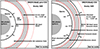 |
Fig. 17. Cartoon of SN 2016adj experiencing a circumstellar interaction (CSI). Left: H-rich shell located within Ds ∼ 0.007 pc of an infant SN delimited with a cavity formed by its progenitor WR wind. The expanding SN ejecta is indicated, along with the CO freshly synthesized within the wake of the SN ejecta. Right: schematic after the shell has been shocked by the expanding SN ejecta. CSI produces both forward and reverse shocks, and the ionization of hydrogen. |
If the origins of the CSM are from a companion star then one would naturally not expect to see any He features. Alternatively, if the CSM originated from the progenitor He could remain hidden due to its high-ionization potential.
8.2. Incidences of H signatures in SNe Ic
The nearby and well-observed type IIb SN 1993J was the first SE SN to exhibit strong evidence of CSI at late phases in the form of Balmer emission features (Filippenko et al. 1994; Patat et al. 1995; Fransson et al. 1996; Houck & Fransson 1996; Chevalier 1997; Matheson et al. 2000). Over the past decade a growing number of SE SNe have been recognized to exhibit (typically late phase) signatures of CSI. In cases of SNe IIb/Ib, these signatures take the form of either CSI emission features, high-ionization coronal features, broadband emission excesses, and/or X-ray emission (e.g., Ben-Ami et al. 2014; Morales-Garoffolo et al. 2014; Maeda et al. 2015; Milisavljevic et al. 2015; Margutti et al. 2017; Mauerhan et al. 2018; Bostroem et al. 2020; Chandra et al. 2020; Kilpatrick et al. 2021; Zenati et al. 2022; Maeda et al. 2023).
Focusing on SNe Ic with claimed CSI produced H signatures, Roy et al. (2016) attributed an excess of flux at peak and the presence of a secondary post-maximum light-curve peak in SN 2012aa to CSI between SN ejecta and a massive H-shell, despite only a tentative detection of Hα. On the other hand, SN 2017dio was the first SN Ic to exhibit prominent hydrogen and helium emission features at early times suggested to be produced from CSI (see Kuncarayakti et al. 2018). CSI driven H emission features and other coronal lines have also been observed in the late phase optical/NIR spectrum of the superluminous type Ic SN 2017ens (Chen et al. 2018), and in the late phase optical spectrum of the bright type Ic-BL SN 2018ijp (Tartaglia et al. 2021).
Recently, the late phase observations of the SN 2021ocs were shown to exhibit features associated with intermediate-mass elements typically not seen in SE SNe (Kuncarayakti et al. 2022). Kuncarayakti et al. (2022) attributed these features to allowed and forbidden transitions of O and Mg which get illuminated by CSI. Most recently, the type Ic-BL SN 2022xxf containing a double hump light curve with each hump reaching the same brightness has also been suggested to experience significant CSI (Kuncarayakti et al. 2023). Finally, Ravi et al. (2023) presented observations on the type Ic SN 2021krf exhibiting an excess of late-phase emission relative to expectations of energy deposition being solely due to 56Co decay. However, due to a lack of CSI spectral features of H, He and/or coronal lines, Ravi et al. (2023) considered the possibilities of an IR echo associated with either pre-existing and/or newly synthesized dust, or emission linked to magnetic dipole radiation from a newly formed neutron star.
Clearly, the time scales and strength of the CSI signatures observed to date in SE SN progenitors suggests a diversity in pre-SN mass-loss histories and underlying progenitor systems. If CSM originates from erupted mass loss of the progenitor star in the lead-up of going core collapse (Dessart et al. 2010; Owocki et al. 2019), Tsuna & Takei (2023) suggest fallback could be suppressed by the star’s radiation pressure. Depending on the amount of ejected material and the radiation pressure of the progenitor star, a cavity devoid of CSM will form around the star. This could account for CSI to naturally occur weeks to months after explosion. A similar effect would also be expected if CSM originated from a companion.
We note that for some SNe (e.g., PTF11iqb, Smith et al. 2015 and iPTF14hls, Andrews & Smith 2018) signatures of late-time CSI have been explained as arising from a disk or torus of CSM that is initially overrun by the SN ejecta, before it is revealed at late times as the optical depth along the line-of-sight drops (Andrews & Smith 2018). In the case of these two objects the late-time Hα line profile showed a distinctive double-peaked emission profile as is expected for an asymmetric geometry; while for SN 2016adj we do not see such a line profile. We cannot exclude a combination of geometry and viewing angle that gives rise to such initially hidden interaction, but equally, there is a lack of evidence in favor of such a scenario.
9. Conclusion
We have presented a detailed analysis of the carbon-rich type Ic SN 2016adj located in the iconic dust lane of the famous early type galaxy Centaurus A. Unsurprisingly, SN 2016adj is found to suffer significant host reddening, preventing an accurate estimate of its peak luminosity and explosion parameters. However, our unique post maximum NIR spectroscopic time series reveals two interesting aspects. The CO first overtone feature appears by +41 days making this the earliest detection in a SN Ic. Modeling of the CO bandhead as captured by two medium-resolution NIR spectra provides an upper limit on the CO mass of MCO ∼ 10−3 M⊙. Secondly, the NIR spectra document the emergence of a handful of P Cygni spectral features that we attribute to H Paschen and Bracket line transitions. These features could arise from CSI between rapidly expanding SN ejecta and a H-rich shell. Such a shell could originate from mass loss experience by the progenitor star in the decades prior to undergoing core-collapse, or alternatively from a companion star which experienced an episode of mass loss. Whatever the origin, the post-maximum H features present in the NIR spectra of SN 2016adj place it among a growing group of SNe Ic, SNe Ic-BL and SLSN-Ic in the literature displaying signatures of CSI involving H-rich material.
A key take away from this study is that medium-resolution NIR spectroscopy offers significant potential to further unravel the pre-SN mass loss history of SE SNe progenitor systems. We therefore recommend future SE SN observational campaigns seek to obtain such data out to late phases. Such observations could serve as a forensic tool to map out the heterogeneous nature of SE SNe mass-loss histories, CSI, and perhaps, a means to disentangle binary versus single star progenitor systems. Fortunately new facilities such as SOXS (son of X-shooter) and NTE (NOT transient explorer) will soon come online, making such data commonplace.
Rest-frame phases of observations are provided throughout, unless explicitly stated, with respect to the epoch of the B-band maximum, which occurred on JD-2457433.5 (see Table 5).
In the spirit of transparency, Fig. A.1 contains sections of the post-maximum NIR spectra with each subpanel centered on the zero velocity of a different Paschen lines.
We briefly explain here why we do not classify SN 2016adj as an SN II. The H lines associated with this object and which we attribute to CSI interaction (see Sect. 8.1) are extremely weak (weaker than C, see Sect. 3.2). It is very unlikely that there are significant amounts of H present in the ejecta, as it is exceedingly difficult to hide hydrogen due to its low ionization potential. The rise time of SN 2016adj is consistent with what is seen in SE SNe, but markedly longer than most SNe II (Sect. 5.2). The emergence of CO at 41 days after maximum (Sect. 3.4) is also similar to what is seen in other SE SNe, and in contrast to the 100 days and later time scales of CO emergence documented in SNe II (Sect. 7.1).
Banerjee et al. (2018) estimated TBB = 3680 K, from a BB fit to a combined optical/NIR spectrum. The discrepancy is largely attributed to their lower adopted host-galaxy color excess of E(B − V)host = 0.60 mag.
Acknowledgments
We appreciate constructive discussions with S. Bose and N. B. Suntzeff. The work of the CSP-II has been generously supported by the National Science Foundation under grants AST-1008343, AST-1613426, AST-1613455, and AST-1613472, and by the Danish Research Foundation via a Sapere Aude Fellowship. M.D.S. is supported by grants from the Independent Research Fund Denmark (IRFD; 8021-00170B and 10.46540/2032-00022B). L.G. acknowledges financial support from the Spanish Ministerio de Ciencia e Innovación (MCIN), the Agencia Estatal de Investigación (AEI) 10.13039/501100011033, and the European Social Fund (ESF) “Investing in your future” under the 2019 Ramón y Cajal program RYC2019-027683-I and the PID2020-115253GA-I00 HOSTFLOWS project, from Centro Superior de Investigaciones Científicas (CSIC) under the PIE project 20215AT016, and the program Unidad de Excelencia María de Maeztu CEX2020-001058-M. This work was funded in part by ANID, Millennium Science Initiative, ICN12_009. MN is supported by the European Research Council (ERC) under the European Union’s Horizon 2020 research and innovation programme (grant agreement No. 948381) and by UK Space Agency Grant No. ST/Y000692/1. This research has made use of the NASA/IPAC Extragalactic Database (NED), which is operated by the Jet Propulsion Laboratory, California Institute of Technology, under contract with the National Aeronautics and Space Administration. Facilities. Based on observations made with facilities at the Las Campanas Observatory including the Swope telescope, the du Pont telescope, and the Magellan telescopes. Data was also obtained with the ESO-La Silla NTT observatory (ESO programme IDs 191.D-0935 and 197.D-1075), the ESO-Paranal VLT (Programme IDs 094.B-0298 and 098.D-0540), and the ESO-Paranal VST (Program ID 60.A-9800). Finally, some data presented were obtained with the Swift Space Telescope. Software: This research made use of Astropy (Price-Whelan et al. 2018) and Photutils (Bradley et al. 2020). Photometry of SN 2016adj was computing using the Aarhus-Barcelona FLOWS projects automated photometry pipeline available for download on https://github.com/SNflows. HYDRA has been used to calculate the CO model spectra, and the gamma-ray transport (Höflich 1990, 2003, 2009; Hristov et al. 2021).
References
- Anderson, J. P. 2019, A&A, 628, A7 [NASA ADS] [CrossRef] [EDP Sciences] [Google Scholar]
- Anderson, J. P., James, P. A., Habergham, S. M., Galbany, L., & Kuncarayakti, H. 2015, PASA, 32, e019 [NASA ADS] [CrossRef] [Google Scholar]
- Andrews, J. E., & Smith, N. 2018, MNRAS, 477, 74 [Google Scholar]
- Arnaboldi, M., Capaccioli, M., Mancini, D., et al. 1998, The Messenger, 93, 30 [NASA ADS] [Google Scholar]
- Arnett, W. D. 1982, ApJ, 253, 785 [Google Scholar]
- Ashall, C., Mazzali, P. A., Pian, E., & James, P. A. 2016, MNRAS, 463, 1891 [NASA ADS] [CrossRef] [Google Scholar]
- Asplund, M., Grevesse, N., Sauval, A. J., & Scott, P. 2009, ARA&A, 47, 481 [NASA ADS] [CrossRef] [Google Scholar]
- Avedisova, V. S. 1972, Sov. Astron., 15, 708 [NASA ADS] [Google Scholar]
- Bacon, R., Vernet, J., Borisova, E., et al. 2014, The Messenger, 157, 13 [NASA ADS] [Google Scholar]
- Banerjee, D. P. K., Connelley, M. S., Tokunaga, A. T., et al. 2016, ATel, 8976, 1 [NASA ADS] [Google Scholar]
- Banerjee, D. P. K., Joshi, V., Evans, A., et al. 2018, MNRAS, 481, 806 [CrossRef] [Google Scholar]
- Barbarino, C., Sollerman, J., Taddia, F., et al. 2021, A&A, 651, A81 [NASA ADS] [CrossRef] [EDP Sciences] [Google Scholar]
- Ben-Ami, S., Gal-Yam, A., Mazzali, P. A., et al. 2014, ApJ, 785, 37 [NASA ADS] [CrossRef] [Google Scholar]
- Bianco, F. B., Modjaz, M., Hicken, M., et al. 2014, ApJS, 213, 19 [Google Scholar]
- Bostroem, K. A., Valenti, S., Sand, D. J., et al. 2020, ApJ, 895, 31 [NASA ADS] [CrossRef] [Google Scholar]
- Bradley, L., Sipőcz, B., Robitaille, T., et al. 2020, https://doi.org/10.5281/zenodo.4044744 [Google Scholar]
- Bransford, M. A., Thilker, D. A., Walterbos, R. A. M., & King, N. L. 1999, AJ, 118, 1635 [NASA ADS] [CrossRef] [Google Scholar]
- Breeveld, A. A., Landsman, W., Holland, S. T., et al. 2011, in Gamma Ray Bursts 2010, eds. J. E. McEnery, J. L. Racusin, & N. Gehrels, AIP Conf. Ser., 1358, 373 [Google Scholar]
- Brown, P. J., Breeveld, A. A., Holland, S., Kuin, P., & Pritchard, T. 2014, Ap&SS, 354, 89 [Google Scholar]
- Brown, P. J., Baron, E., Milne, P., Roming, P. W. A., & Wang, L. 2015, ApJ, 809, 37 [NASA ADS] [CrossRef] [Google Scholar]
- Buzzoni, B., Delabre, B., Dekker, H., et al. 1984, The Messenger, 38, 9 [NASA ADS] [Google Scholar]
- Cappa, C., Niemela, V. S., Martín, M. C., & McClure-Griffiths, N. M. 2005, A&A, 436, 155 [NASA ADS] [CrossRef] [EDP Sciences] [Google Scholar]
- Chandra, P., Chevalier, R. A., Chugai, N., Milisavljevic, D., & Fransson, C. 2020, ApJ, 902, 55 [NASA ADS] [CrossRef] [Google Scholar]
- Chen, T. W., Inserra, C., Fraser, M., et al. 2018, ApJ, 867, L31 [NASA ADS] [CrossRef] [Google Scholar]
- Chevalier, R. A. 1997, Science, 276, 1374 [NASA ADS] [CrossRef] [Google Scholar]
- Chevalier, R. A., & Fransson, C. 1994, ApJ, 420, 268 [NASA ADS] [CrossRef] [Google Scholar]
- Chu, Y. H. 1981, ApJ, 249, 195 [NASA ADS] [CrossRef] [Google Scholar]
- Cid Fernandes, R., Mateus, A., Sodré, L., Stasińska, G., & Gomes, J. M. 2005, MNRAS, 358, 363 [Google Scholar]
- Crowther, P. A. 2007, ARA&A, 45, 177 [Google Scholar]
- Das, R. K., Banerjee, D. P. K., & Ashok, N. M. 2009, MNRAS, 398, 375 [NASA ADS] [CrossRef] [Google Scholar]
- Davis, S., Hsiao, E. Y., Ashall, C., et al. 2019, ApJ, 887, 4 [NASA ADS] [CrossRef] [Google Scholar]
- de Jaeger, T., Zheng, W., Stahl, B. E., et al. 2019, MNRAS, 490, 2799 [NASA ADS] [CrossRef] [Google Scholar]
- Della Valle, M., & Panagia, N. 2003, ApJ, 587, L71 [NASA ADS] [CrossRef] [Google Scholar]
- Della Valle, M., Panagia, N., Padovani, P., et al. 2005, ApJ, 629, 750 [CrossRef] [Google Scholar]
- Dessart, L., Livne, E., & Waldman, R. 2010, MNRAS, 405, 2113 [NASA ADS] [Google Scholar]
- Dopita, M. A., Kewley, L. J., Sutherland, R. S., & Nicholls, D. C. 2016, Ap&SS, 361, 61 [NASA ADS] [CrossRef] [Google Scholar]
- Dressler, A., Bigelow, B., Hare, T., et al. 2011, PASP, 123, 288 [NASA ADS] [CrossRef] [Google Scholar]
- Drout, M. R., Soderberg, A. M., Gal-Yam, A., et al. 2011, ApJ, 741, 97 [NASA ADS] [CrossRef] [Google Scholar]
- Drout, M. R., Milisavljevic, D., Parrent, J., et al. 2016, ApJ, 821, 57 [NASA ADS] [CrossRef] [Google Scholar]
- Eldridge, J. J., Fraser, M., Smartt, S. J., Maund, J. R., & Crockett, R. M. 2013, MNRAS, 436, 774 [NASA ADS] [CrossRef] [Google Scholar]
- Ergon, M., Sollerman, J., Fraser, M., et al. 2014, A&A, 562, A17 [NASA ADS] [CrossRef] [EDP Sciences] [Google Scholar]
- Ferrarese, L., Mould, J. R., Stetson, P. B., et al. 2007, ApJ, 654, 186 [Google Scholar]
- Filippenko, A. V., Matheson, T., & Barth, A. J. 1994, AJ, 108, 2220 [NASA ADS] [CrossRef] [Google Scholar]
- Fitzpatrick, E. L. 1999, PASP, 111, 63 [Google Scholar]
- Fouque, P., Gourgoulhon, E., Chamaraux, P., & Paturel, G. 1992, A&AS, 93, 211 [NASA ADS] [Google Scholar]
- Fransson, C., Lundqvist, P., & Chevalier, R. A. 1996, ApJ, 461, 993 [NASA ADS] [CrossRef] [Google Scholar]
- Galbany, L., Mora, L., González-Gaitán, S., et al. 2017, MNRAS, 468, 628 [NASA ADS] [CrossRef] [Google Scholar]
- Galbany, L., Anderson, J. P., Sánchez, S. F., et al. 2018, ApJ, 855, 107 [Google Scholar]
- Gehrels, N., Chincarini, G., Giommi, P., et al. 2004, ApJ, 611, 1005 [Google Scholar]
- Goobar, A. 2008, ApJ, 686, L103 [CrossRef] [Google Scholar]
- Grosdidier, Y., Moffat, A. F. J., Joncas, G., & Acker, A. 1998, ApJ, 506, L127 [NASA ADS] [CrossRef] [Google Scholar]
- Gutiérrez, C. P., Bersten, M. C., Orellana, M., et al. 2021, MNRAS, 504, 4907 [CrossRef] [Google Scholar]
- Gutiérrez, C. P., Pastorello, A., Bersten, M., et al. 2022, MNRAS, 517, 2056 [CrossRef] [Google Scholar]
- Hamuy, M., Folatelli, G., Morrell, N. I., et al. 2006, PASP, 118, 2 [NASA ADS] [CrossRef] [Google Scholar]
- Harris, G. L. H. 2010, PASA, 27, 475 [NASA ADS] [CrossRef] [Google Scholar]
- Hicken, M., Friedman, A. S., Blondin, S., et al. 2017, ApJS, 233, 6 [NASA ADS] [CrossRef] [Google Scholar]
- Hoeflich, P., Ashall, C., Bose, S., et al. 2021, ApJ, 922, 186 [NASA ADS] [CrossRef] [Google Scholar]
- Höflich, P. 1990, PhD Thesis, Ludwig-Maximilians-Universität, Munich, Germany [Google Scholar]
- Höflich, P. 2003, in Stellar Atmosphere Modeling, eds. I. Hubeny, D. Mihalas, & K. Werner, ASP Conf. Ser., 288, 371 [Google Scholar]
- Höflich, P. 2009, in Recent Directions in Astrophysical Quantitative Spectroscopy and Radiation Hydrodynamics, eds. I. Hubeny, J. M. Stone, K. MacGregor, & K. Werner, AIP Conf. Ser., 1171, 161 [Google Scholar]
- Holmbo, S., Stritzinger, M. D., Karamehmetoglu, E., et al. 2023, A&A, 675, A83 [NASA ADS] [CrossRef] [EDP Sciences] [Google Scholar]
- Houck, J. C., & Fransson, C. 1996, ApJ, 456, 811 [NASA ADS] [CrossRef] [Google Scholar]
- Hough, J. H., Bailey, J. A., Rouse, M. F., & Whittet, D. C. B. 1987, MNRAS, 227, 1P [NASA ADS] [CrossRef] [Google Scholar]
- Hounsell, R. A., Miller, J. A., Pan, Y. C., et al. 2016, ATel, 8663, 1 [NASA ADS] [Google Scholar]
- Hristov, B., Hoeflich, P., & Collins, D. C. 2021, ApJ, 923, 210 [NASA ADS] [CrossRef] [Google Scholar]
- Hsiao, E. Y., Phillips, M. M., Marion, G. H., et al. 2019, PASP, 131, 014002 [NASA ADS] [CrossRef] [Google Scholar]
- Hunter, D. J., Valenti, S., Kotak, R., et al. 2009, A&A, 508, 371 [NASA ADS] [CrossRef] [EDP Sciences] [Google Scholar]
- Israel, F. P. 1998, A&A Rev., 8, 237 [Google Scholar]
- Jiménez-Hernández, P., Arthur, S. J., & Toalá, J. A. 2020, MNRAS, 497, 4128 [CrossRef] [Google Scholar]
- Johnson, H. M., & Hogg, D. E. 1965, ApJ, 142, 1033 [NASA ADS] [CrossRef] [Google Scholar]
- Kasen, D., & Bildsten, L. 2010, ApJ, 717, 245 [NASA ADS] [CrossRef] [Google Scholar]
- Kelly, P. L., Ciardi, D. R., Beichman, C. A., et al. 2016, ATel, 8720, 1 [NASA ADS] [Google Scholar]
- Kennicutt, R. C., Jr 1998, ApJ, 498, 541 [Google Scholar]
- Khatami, D. K., & Kasen, D. N. 2019, ApJ, 878, 56 [NASA ADS] [CrossRef] [Google Scholar]
- Kilpatrick, C. D., Drout, M. R., Auchettl, K., et al. 2021, MNRAS, 504, 2073 [CrossRef] [Google Scholar]
- Kiyota, S., Shappee, B. J., Stanek, K. Z., & Dong, S. 2016, ATel, 8654, 1 [NASA ADS] [Google Scholar]
- Krisciunas, K., Contreras, C., Burns, C. R., et al. 2017, AJ, 154, 211 [NASA ADS] [CrossRef] [Google Scholar]
- Krühler, T., Kuncarayakti, H., Schady, P., et al. 2017, A&A, 602, A85 [NASA ADS] [CrossRef] [EDP Sciences] [Google Scholar]
- Kuijken, K. 2011, The Messenger, 146, 8 [NASA ADS] [Google Scholar]
- Kuijken, K., Bender, R., Cappellaro, E., et al. 2002, The Messenger, 110, 15 [NASA ADS] [Google Scholar]
- Kuncarayakti, H., Maeda, K., Ashall, C. J., et al. 2018, ApJ, 854, L14 [NASA ADS] [CrossRef] [Google Scholar]
- Kuncarayakti, H., Maeda, K., Dessart, L., et al. 2022, ApJ, 941, L32 [NASA ADS] [CrossRef] [Google Scholar]
- Kuncarayakti, H., Sollerman, J., Izzo, L., et al. 2023, A&A, 678, A209 [NASA ADS] [CrossRef] [EDP Sciences] [Google Scholar]
- Landolt, A. U. 1992, AJ, 104, 340 [Google Scholar]
- Lyman, J. D., Bersier, D., & James, P. A. 2014, MNRAS, 437, 3848 [Google Scholar]
- Lyman, J. D., Bersier, D., James, P. A., et al. 2016, MNRAS, 457, 328 [Google Scholar]
- Lyman, J. D., Taddia, F., Stritzinger, M. D., et al. 2018, MNRAS, 473, 1359 [NASA ADS] [CrossRef] [Google Scholar]
- Lynch, D. K., Rudy, R. J., Mazuk, S., & Puetter, R. C. 2000, ApJ, 541, 791 [NASA ADS] [CrossRef] [Google Scholar]
- Maeda, K., Hattori, T., Milisavljevic, D., et al. 2015, ApJ, 807, 35 [NASA ADS] [CrossRef] [Google Scholar]
- Maeda, K., Chandra, P., Moriya, T. J., et al. 2023, ApJ, 942, 17 [NASA ADS] [CrossRef] [Google Scholar]
- Marchenko, S. V., Moffat, A. F. J., & Crowther, P. A. 2010, ApJ, 724, L90 [NASA ADS] [CrossRef] [Google Scholar]
- Margutti, R., Kamble, A., Milisavljevic, D., et al. 2017, ApJ, 835, 140 [NASA ADS] [CrossRef] [Google Scholar]
- Marino, R. A., Rosales-Ortega, F. F., Sánchez, S. F., et al. 2013, A&A, 559, A114 [NASA ADS] [CrossRef] [EDP Sciences] [Google Scholar]
- Marples, P., Bock, G., & Parker, S. 2016, ATel, 8651, 1 [NASA ADS] [Google Scholar]
- Massey, P. 2002, ApJS, 141, 81 [NASA ADS] [CrossRef] [Google Scholar]
- Matheson, T., Filippenko, A. V., Ho, L. C., Barth, A. J., & Leonard, D. C. 2000, AJ, 120, 1499 [NASA ADS] [CrossRef] [Google Scholar]
- Mathis, J. S. 1990, ARA&A, 28, 37 [NASA ADS] [CrossRef] [Google Scholar]
- Mauerhan, J. C., Filippenko, A. V., Zheng, W., et al. 2018, MNRAS, 478, 5050 [NASA ADS] [CrossRef] [Google Scholar]
- Maund, J. R., Fraser, M., Reilly, E., Ergon, M., & Mattila, S. 2015, MNRAS, 447, 3207 [CrossRef] [Google Scholar]
- Milisavljevic, D., Margutti, R., Kamble, A., et al. 2015, ApJ, 815, 120 [NASA ADS] [CrossRef] [Google Scholar]
- Millard, J., Branch, D., Baron, E., et al. 1999, ApJ, 527, 746 [NASA ADS] [CrossRef] [Google Scholar]
- Modjaz, M., Blondin, S., Kirshner, R. P., et al. 2014, AJ, 147, 99 [Google Scholar]
- Moorwood, A., Cuby, J. G., & Lidman, C. 1998, The Messenger, 91, 9 [Google Scholar]
- Morales-Garoffolo, A., Elias-Rosa, N., Benetti, S., et al. 2014, MNRAS, 445, 1647 [Google Scholar]
- Müller, B. 2016, PASA, 33, e048 [Google Scholar]
- Omand, C. M. B., & Sarin, N. 2024, MNRAS, 527, 6455 [Google Scholar]
- Osterbrock, D. E., & Ferland, G. J. 2006, Astrophysics of Gseous Nebulae and Active Galactic Nuclei (Mill Valley: University Science Books) [Google Scholar]
- Owocki, S. P., Hirai, R., Podsiadlowski, P., & Schneider, F. R. N. 2019, MNRAS, 485, 988 [NASA ADS] [CrossRef] [Google Scholar]
- Patat, F., Chugai, N., & Mazzali, P. A. 1995, A&A, 299, 715 [NASA ADS] [Google Scholar]
- Patat, F., Taubenberger, S., Cox, N. L. J., et al. 2015, A&A, 577, A53 [NASA ADS] [CrossRef] [EDP Sciences] [Google Scholar]
- Persson, S. E., Murphy, D. C., Krzeminski, W., Roth, M., & Rieke, M. J. 1998, AJ, 116, 2475 [NASA ADS] [CrossRef] [Google Scholar]
- Phillips, M. M. 1993, ApJ, 413, L105 [Google Scholar]
- Phillips, M. M., Phillips, A. C., Heathcote, S. R., et al. 1987, PASP, 99, 592 [NASA ADS] [CrossRef] [Google Scholar]
- Phillips, M. M., Simon, J. D., Morrell, N., et al. 2013, ApJ, 779, 38 [NASA ADS] [CrossRef] [Google Scholar]
- Phillips, M. M., Contreras, C., Hsiao, E. Y., et al. 2019, PASP, 131, 014001P [NASA ADS] [CrossRef] [Google Scholar]
- Podsiadlowski, P., Ivanova, N., Justham, S., & Rappaport, S. 2010, MNRAS, 406, 840 [NASA ADS] [Google Scholar]
- Prentice, S. J., Mazzali, P. A., Pian, E., et al. 2016, MNRAS, 458, 2973 [NASA ADS] [CrossRef] [Google Scholar]
- Prentice, S. J., Ashall, C., James, P. A., et al. 2019, MNRAS, 485, 1559 [NASA ADS] [CrossRef] [Google Scholar]
- Price-Whelan, A., Crawford, S., Sipocz, B., et al. 2018, https://doi.org/10.5281/zenodo.1211397 [Google Scholar]
- Puls, J., Vink, J. S., & Najarro, F. 2008, A&A Rev., 16, 209 [NASA ADS] [CrossRef] [Google Scholar]
- Rate, G., & Crowther, P. A. 2020, MNRAS, 493, 1512 [NASA ADS] [CrossRef] [Google Scholar]
- Ravi, A. P., Rho, J., Park, S., et al. 2023, ApJ, 950, 14 [CrossRef] [Google Scholar]
- Roming, P. W. A., Kennedy, T. E., Mason, K. O., et al. 2005, Space Sci. Rev., 120, 95 [Google Scholar]
- Roy, R., Sollerman, J., Silverman, J. M., et al. 2016, A&A, 596, A67 [NASA ADS] [CrossRef] [EDP Sciences] [Google Scholar]
- Rybicki, G. B., & Lightman, A. P. 1979, Radiative Processes in Astrophysics (New York: Wiley) [Google Scholar]
- Schlafly, E. F., & Finkbeiner, D. P. 2011, ApJ, 737, 103 [Google Scholar]
- Schrøder, S. L., MacLeod, M., Loeb, A., Vigna-Gómez, A., & Mandel, I. 2020, ApJ, 892, 13 [CrossRef] [Google Scholar]
- Sextl, E., Kudritzki, R.-P., Zahid, H. J., & Ho, I. T. 2023, ApJ, 949, 60 [NASA ADS] [CrossRef] [Google Scholar]
- Shahbandeh, M., Hsiao, E. Y., Ashall, C., et al. 2022, ApJ, 925, 175 [NASA ADS] [CrossRef] [Google Scholar]
- Simcoe, R. A., Burgasser, A. J., Schechter, P. L., et al. 2013, PASP, 125, 270 [NASA ADS] [CrossRef] [Google Scholar]
- Simon, M., & Axford, W. I. 1966, Planet Space Sci., 14, 901 [NASA ADS] [CrossRef] [Google Scholar]
- Skrutskie, M. F., Cutri, R. M., Stiening, R., et al. 2006, AJ, 131, 1163 [NASA ADS] [CrossRef] [Google Scholar]
- Smartt, S. J., Valenti, S., Fraser, M., et al. 2015, A&A, 579, A40 [NASA ADS] [CrossRef] [EDP Sciences] [Google Scholar]
- Smith, L. F. 1967, AJ, 72, 829 [NASA ADS] [CrossRef] [Google Scholar]
- Smith, N., & Arnett, W. D. 2014, ApJ, 785, 82 [NASA ADS] [CrossRef] [Google Scholar]
- Smith, J. A., Tucker, D. L., Kent, S., et al. 2002, AJ, 123, 2121 [NASA ADS] [CrossRef] [Google Scholar]
- Smith, N., Mauerhan, J. C., Cenko, S. B., et al. 2015, MNRAS, 449, 1876 [Google Scholar]
- Sollerman, J., Yang, S., Perley, D., et al. 2022, A&A, 657, A64 [NASA ADS] [CrossRef] [EDP Sciences] [Google Scholar]
- Stritzinger, M., Mazzali, P., Phillips, M. M., et al. 2009, ApJ, 696, 713 [NASA ADS] [CrossRef] [Google Scholar]
- Stritzinger, M., Hsiao, E. Y., Morrell, N., et al. 2016, ATel, 8657, 1 [NASA ADS] [Google Scholar]
- Stritzinger, M. D., Taddia, F., Burns, C. R., et al. 2018, A&A, 609, A135 [NASA ADS] [CrossRef] [EDP Sciences] [Google Scholar]
- Stritzinger, M. D., Taddia, F., Lawrence, S. S., et al. 2022, ApJ, 939, L8 [CrossRef] [Google Scholar]
- Taddia, F., Sollerman, J., Leloudas, G., et al. 2015, A&A, 574, A60 [NASA ADS] [CrossRef] [EDP Sciences] [Google Scholar]
- Taddia, F., Fremling, C., Sollerman, J., et al. 2016, A&A, 592, A89 [NASA ADS] [CrossRef] [EDP Sciences] [Google Scholar]
- Taddia, F., Sollerman, J., Fremling, C., et al. 2018a, A&A, 609, A106 [NASA ADS] [CrossRef] [EDP Sciences] [Google Scholar]
- Taddia, F., Stritzinger, M. D., Bersten, M., et al. 2018b, A&A, 609, A136 [NASA ADS] [CrossRef] [EDP Sciences] [Google Scholar]
- Tartaglia, L., Sollerman, J., Barbarino, C., et al. 2021, A&A, 650, A174 [NASA ADS] [CrossRef] [EDP Sciences] [Google Scholar]
- Thomas, A., Tucker, B. E., Childress, M., et al. 2016, ATel, 8664, 1 [NASA ADS] [Google Scholar]
- Tonry, J. L., Denneau, L., Flewelling, H., et al. 2018, ApJ, 867, 105 [NASA ADS] [CrossRef] [Google Scholar]
- Tsuna, D., & Takei, Y. 2023, PASJ, 75, L19 [NASA ADS] [CrossRef] [Google Scholar]
- Tuthill, P., Monnier, J., Tanner, A., et al. 2006, Science, 313, 935 [NASA ADS] [CrossRef] [Google Scholar]
- Valenti, S., Elias-Rosa, N., Taubenberger, S., et al. 2008, ApJ, 673, L155 [NASA ADS] [CrossRef] [Google Scholar]
- Valenti, S., Taubenberger, S., Pastorello, A., et al. 2012, ApJ, 749, L28 [NASA ADS] [CrossRef] [Google Scholar]
- Valenti, S., Howell, D. A., Stritzinger, M. D., et al. 2016, MNRAS, 459, 3939 [NASA ADS] [CrossRef] [Google Scholar]
- Vink, J. S. 2017, Phil. Trans. Royal Soc. London Ser. A, 375, 20160269 [Google Scholar]
- Williams, P. M., Morrell, N. I., Boutsia, K., & Massey, P. 2021, MNRAS, 505, 5029 [CrossRef] [Google Scholar]
- Yaron, O., & Gal-Yam, A. 2012, PASP, 124, 668 [Google Scholar]
- Yi, W., Zhang, J.-J., Wu, X.-B., et al. 2016, ATel, 8655, 1 [NASA ADS] [Google Scholar]
- Yoon, S.-C. 2017, MNRAS, 470, 3970 [NASA ADS] [CrossRef] [Google Scholar]
- Zavala, S., Toalá, J. A., Santamaría, E., et al. 2022, MNRAS, 513, 3317 [NASA ADS] [CrossRef] [Google Scholar]
- Zenati, Y., Wang, Q., Bobrick, A., et al. 2022, ApJ, submitted [arXiv:2207.07146] [Google Scholar]
Appendix A: Observations and data reductions
A.1. CSP-II observations
We collected an extensive set of ground-based optical and NIR photometry and spectroscopy of SN 2016adj. The bulk of the data were obtained by the Carnegie Supernova Project-II (Phillips et al. 2019, hereafter CSP-II) and the Public ESO Spectroscopic Survey of Transient Objects (Smartt et al. 2015, hereafter PESSTO). Finally, we identified a detection of SN 2016adj recovered in a single VST i-band image obtained nearly two weeks prior to the original discovery by BOSS.
The CSP-II obtained detailed followup spectroscopy and photometry using key facilities located on the Las Campanas Observatory (LCO). As summarized in Table 1, CSP-II obtained nine epochs of optical spectra with the du Pont telescope equipped with the B&C and WFCCD spectrographs, the Magellan BAADE telescope equipped with IMACS (Inamori-Magellan Areal Camera & Spectrograph; Dressler et al. 2011), and the Magellan Baade telescope equipped with MagE (Magellan Echellette) and LDSS3 (Low Dispersion Survey Spectrograph). These data were reduced in the IRAF environment following standard procedures as outlined by Hamuy et al. (2006).
The CSP-II also obtained 6 epochs of NIR spectroscopy with the FIRE (Folded port InfraRed Echellette; Simcoe et al. 2013) spectrograph attached to the Magellan BAADE telescope. Four of these spectra were obtained in low-resolution mode, while two were obtained in echelle mode providing higher spectral resolution. The lower resolution data were reduced following procedures outlined by Hsiao et al. (2019), while the FIRE/echelle spectra were reduce using the FIREHOSE IDL pipeline provided by the instrument developer R. Simcoe (Simcoe et al. 2013).
As the detection of hydrogen features in the NIR spectra of SN 2016adj are of significant interest, particular attention was paid to investigate whether or not the purported P Cygni hydrogen features detected in the +97 days medium-resolution spectrum (see Fig. 5) are intrinsic and not simply an artifact of the telluric correction. The +97 days NIR spectrum was telluric corrected using observations of the telluric standard star HIP 64381 obtained just after the science data. Indeed, at times the kernel constructed from the Pa-δ feature of this star can lead to corrections that leave residual artefacts, however, not with the relative intensities of the features present in the science spectrum. Turning to the +159 days echelle spectrum unfortunately no telluric spectrum was obtained, and therefore that used in the previous echelle spectral data reductions was used, which provided adequate telluric removal. Visual inspection of the 2D science images of both echelle nights reveal obvious features at the location of the detected hydrogen features. Furthermore, any artefacts related to telluric removal would not be accompanied by P Cygni profiles, and if present the artefacts would be located at zero red-shift, which in the rest-frame of Centaurus A would be around −500 km s−1. This is inconsistent with the line velocities of the NIR lines highlighted in Fig. 5. In connection with Fig. 5, plotted in Fig. A.1 are post-maximum NIR spectra of SN 2016adj with each subpanel centered on the zero velocity of a different Paschen lines.
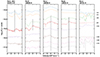 |
Fig. A.1. Sections of post maximum NIR spectra of SN 2016adj plotted in velocity space and centered on the rest wavelengths of five Paschen spectral lines. Vertical dashed lines coincide with the spectra exhibiting Paschen features in Pa-δ, Pa-γ, and Pa-β. For Pa-ζ, it indicates a potential detection, whereas Pa-α lacks evidence of a feature (see Table 3 for a summary of line identifications). |
Turning to the broadband imaging of SN 2016adj, depending on the particular band, up to 30 epochs of optical (uBgVri) photometry were obtained with the 1-m Swope telescope equipped with a e2v CCD. The CSP-II also obtained 8 epochs of broad-band NIR (YJH) imaging with the 2.5-m du Pont telescope equipped with the NIR imager RetroCam containing a Rochwell HAWAII-1 HgCdTe detector. These data were reduced as described by Krisciunas et al. (2017, and references therein).
The bright star in close vicinity of the position of SN 2016adj posed significant issues to standard template subtraction and PSF photometry techniques. After extensive trial and error, optimal results were obtained following the approach illustrated in Fig. A.2. First, for each stacked science image (top left) a PSF model constructed from field stars was subtracted from the PSF of the bright star, resulting in a residual of it (top right). This residual is then masked (bottom right), and then host-galaxy template subtraction is performed yielding a suitable data product (bottom left) to measure the brightness of the SN free of both contamination by the bright star and the underlying host-galaxy light.
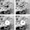 |
Fig. A.2. Steps of host-galaxy template subtraction. Top left: Optical-band science image created from stacking multiple images and zoomed in on the location of SN 2016adj. North is up and east is to the left. Top right: Residual obtained after subtraction of a modeled PSF from the PSF of the bright foreground star located in close proximity to SN 2016adj. Bottom right: Mask applied to the residual of the bright star. Bottom left: Region surrounding SN 2016adj copied into the initial science image after performing host-galaxy template subtraction of the masked science image. |
PSF photometry of SN 2016adj was computed differential relative to a local sequence of secondary standard stars. These secondary standards were themselves calibrated relative to standard star fields observed over multiple photometric nights and with photometry presented by Landolt (1992) (BV), Smith et al. (2002) (ugri), Krisciunas et al. (2017) (Y), and Persson et al. (1998) (JH). In order to compute photometry of the SN in the natural photometric system, which represents the purest form of the data, the published standard star magnitudes were converted to the CSP-II natural system following the relation (using the B band as an example): Bnat = BSTD + CTB(BSTD − VSTD), where color term values are taken from Table 4 of Krisciunas et al. (2017).
For reference, photometry of the optical (uBgVri) and NIR (YJH) secondary standards in the standard system is provided in Tables A.1 and A.2, respectively. All photometry presented in this work was computed using the PYTHON-based photometry pipeline developed by the Aarhus-Barcelona FLOWS6 project and available on GITHUB7.
Optical photometry of the local sequence in the Swope ‘natural’ system.
CSP-II NIR local sequence photometry of SN 2016adj in the ‘standard’ system.
Final natural system optical and NIR photometry of SN 2016adj obtained by CSP-II is listed in Table A.3 with accompanying 1-σ uncertainties computed by adding in quadrature the PSF-photometry error and the nightly zero-point error.
Ground-based photometry of SN 2016adj.
A.2. PESSTO observations
PESSTO obtained optical-NIR photometry and spectroscopy with the ESO-La Silla Observatory’s 3.4-m New Technology Telescope (NTT), equipped with EFOSC2 (ESO Faint Object Spectrograph and Camera; Buzzoni et al. 1984) and Sofi (Son Of ISAAC; Moorwood et al. 1998). The data set includes 5 optical spectra, 7 NIR spectra, several epochs of uBgVri-band photometry, and up to 7 epochs of NIR photometry. Reductions of the data were performed following the procedures outlined in the PESSTO survey paper (Smartt et al. 2015).
Prior to computing photometry of the EFOSC2 science images, each image went through the same arduous template-subtraction process described in Sect. A.1 and summarized in Fig. A.2. Due to the limited field-of-view afforded by EFOSC2 and Sofi the local sequences defined in Sect. A.1 and used with the CSP-II images were not suitable to compute nightly zero-points. Nightly optical and NIR zeropoints were therefore computed relative to ATLAS-REFCAT2 (Tonry et al. 2018) and 2MASS (Skrutskie et al. 2006) stars contained within each of the PESSTO science images. In the optical the number of calibration stars typically consisted of (depending on the filter and exposure time) between ∼30-50, while in the NIR the number of calibrating stars was typically ≳30. Prior to computing the optical local night zeropoints the photometry of the calibrating stars was transformed to the NTT (+EFOSC2) natural system using color terms provided by Smartt et al. (2015). The resulting photometry is listed in Table A.3.
We now turn to a tentative feature appearing just bluewards of the rest wavelength of Hα in the optical spectra obtained between 31 days and 43 days post the epoch of the B-band maximum (see Fig. 2). During these post maximum phases the optical spectroscopic data are significantly contaminated around the rest wavelength of Hα alpha due to underlying host emission. As a result, the IRAF extraction task APALL struggles to fit and remove host contamination. The significant background relative to emission leads to poor host subtraction and yields a subtracted spectrum with a P Cygni-like feature in the spectra extending between 31 to 49 days.
To illustrate this problem, we used the EFOSC2 spectrum taken on 2016 April 4.3 UT to investigate the effect of background contamination on the extracted spectrum in the region around Hα. When no background subtraction is performed, a strong narrow emission peak is seen at the rest wavelength of Hα. This is illustrated in the top spectrum in the right panel of Fig. A.3. We then made a careful background subtraction using the IRAF APALL task as shown in Fig. A.3. We find that regardless of the precise region used to measure the background flux when extracting the one-dimensional spectrum, a weak narrow (i.e., unresolved) absorption line remains at the rest wavelength of Hα. A second, weak absorption is also evident in these spectra located roughly 1,500 km s−1 bluewards of the rest wavelength of Hα. It is uncertain whether this is a real feature, and if so, there is further uncertain if it is associated with Hα or another ion. We therefore pseudo-mask this feature in the 31 to 49 days spectra plotted in Fig. 2.
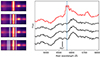 |
Fig. A.3. Shown in the right panel is the NTT +EFOSC2 one-dimensional spectrum obtained on 2016 April 4.3 UT and extracted without background subtraction (red), and with background subtraction (black) using three slightly different background regions, as indicated in the left panels. Each of the extracted spectra reveals a feature which if associated with Hα would imply a −vabs = 1, 500 km s−1. |
A.3. ESO VST early i-band image of SN 2016adj
SN 2016adj was recovered in a single i-band image taken on 2016 January 26.3 UT with the ESO-Paranal VLT Survey Telescope (VST), equipped with the wide-field imaging camera OmegaCAM (Arnaboldi et al. 1998; Kuijken et al. 2002; Kuijken 2011). The date of this observation turns out to be −19.9 days prior to the epoch of the B-band maximum, and only a mere +2.5 days past our inferred explosion epoch (see Sect. 5). This epoch is also 13.28 days prior to the reported date of discovery (Marples et al. 2016). Template subtraction was performed on the science image as described above and PSF photometry was computed deferentially relative to 100 ATLAS-REFCAT2 stars contained within the field of the science image.
A.4. ESO VLT X-shooter observations
The X-Shooter medium-resolution spectrograph attempted to obtain late-phase spectroscopy (ESO program 098.D-0540(A)) of SN 2016adj at late phases. Unfortunately, the four 1-hour observational blocks executed between 2017 February 03.2 UT and 2017 April 01.1 UT contained no useful science data.
A.5. Pre-maximum Swift/UVOT followup
Over the first twenty-four hours after the reported discovery several snapshot observations of SN 2016adj were obtained with the UVOT camera (Roming et al. 2005) onboard the Neil Gehrels Swift Observatory (Gehrels et al. 2004). Due to the significant host reddening, SN 2016adj was only detected in the uvw1, U, B, and V bands. However, due to the high-galaxy background it was not possible to obtain reliable photometry for the optical detections. Furthermore, uvw2 was not considered because reddened sources such as SN 2016adj are dominated by the red tail of this UV filter. In summary, out of the initial Swift observations, only a single uvw1 point a few days before B-band maximum is recovered, as well as two upper limits for both the uvw1 and uvm2 bands around −6 days. Aperture photometry was computed at the position of SN 2016adj following the method used for the Swift Optical Ultraviolet Supernova Archive (SOUSA; Brown et al. 2014). The underlying galaxy count rates were subtracted from the science flux measurements and photometry was computed using a 5″ aperture along with the Swift/UVOT Vega-based photometric zeropoints (Breeveld et al. 2011) and the most recent sensitivity corrections.8 The single UVOT photometry measurement as well as several limits are listed in Table A.4. The uvw1 measurement must be used with the understanding that the effective wavelength is shifted redward as SN 2016adj is such a red and reddened source (Brown et al. 2015).
Swift photometry of SN 2016adj.
Appendix B: On the local environment of SN 2016adj in the dust lane of Centaurus A
The position of SN 2016adj was previously observed with the ESO-Paranal VLT equipped with the MUSE (Multi Unit Spectroscopic Explorer; Bacon et al. 2014) instrument on 2015 January 25 (PI J. Walcher, ESO Program ID 094.B-0298). A single pointing of 295 seconds covering the coordinates of SN 2016adj was identified within the ESO archive providing a field-of-view (FOV) of 1 arcmin. We now summarize the data reduction and analysis techniques used to estimate values related to the gas phase  color excess, the metallicity, and star formation rate.
As a first step the MUSE data cube was downloaded from the ESO archive and basic data reductions were performed following the procedures presented by Krühler et al. (2017). To analyze the data cube we followed the method described by Lyman et al. (2018, see also Galbany et al. 2018 and references therein) making extensive use of the PYTHON package IFUANAL9. IFUANAL performs spaxel binning by growing bins from initial peaks in a Hα map based on some constraints on pixel values and weighted distances to their respective peaks. Once all individual spectra in the data cube were combined in the bins provided by the segmentation routine, the associated stellar continuum and emission lines were fit with the stellar population package STARLIGHT (Cid Fernandes et al. 2005), revealing a best-fit stellar population model (SSP). The stellar population model was then removed from each spaxel spectrum, resulting in a pure gas-emission spectrum.
Armed with the pure gas phase spectra for each spaxel region, a Gaussian function was fit to the strongest emission lines, including Hα, Hβ, [O III] λ5007, [N II] λ6583, and the [S II] λλ6719,6731 doublet.
The Balmer decrement was measured and assuming case B recombination with the canonical Hα-to-Hβ ratio of 2.86 (Osterbrock & Ferland 2006),  was inferred. The extinction-corrected line flux measurements were then used to estimate both the star-formation rate density (ΣSFR) and the gas-phase metallicity (12 + log(O/H)) using published O3N2 calibrations (e.g., Marino et al. 2013; Dopita et al. 2016). Finally, the stellar population model is also used to normalize the extracted spectra to enable an Hα equivalent width measurement, which provides an assessment of the prevalence of young stellar populations relative to the older stellar content.
The results of this analysis are summarized in the multi-panel plot shown in Fig. B.1. Contained within the various panels are the spatial segmentation regions overlaid with the analysis mappings including: the observed Hα flux (panel 1), the  map (panel 2), and the O3N2 gas-phase metallicity maps inferred from the Marino et al. (2013) (panel 3) and Dopita et al. (2016) (panel 4) calibrations. We note that in each panel the location of the SN is marked with a star symbol, while the center of the H II-region’s peak emission within each segmented region is marked with a cross. Also, the location of the bright foreground star in close proximity of the location of SN 2016adj is masked with a filled orange circle, and this region was excluded from the entire analysis.
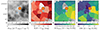 |
Fig. B.1. Spaxel binned MUSE data cube revealing (from left to right) the Hα flux (panel 1), the Balmer decrement-based |

The extinction map suggests for the bin containing the location of SN 2016adj a color excess  mag. Moreover, the O3N2 gas phase metallicity of this bin is measured to be (12 + log(O/H)) = 8.55 ± 0.18 dex (panel 3) and 8.67 ± 0.18 dex (panel 4). These estimates are consistent with the solar value of (12 + log(O/H)) = 8.7 ± 0.2 dex (Asplund et al. 2009). We also obtained a Hα equivalent width of 54±2 Å, and a ΣSFR = 3.47±0.13×10⁻⁴ M⊙ yr−1 kpc−2 using the Kennicutt (1998) relation. This ΣSFR lays in the bottom 10% of the 66 stripped-envelope SN environments in the PISCO compilation (Galbany et al. 2018).
In addition to the segmented regions, the same analysis was applied to a spectrum extracted from the data cube using a seeing-diameter aperture centered on the coordinates of SN 2016adj. The extracted 1D spectrum is plotted in Fig. B.2, together with the best STARLIGHT fit, and the subtraction of the two, revealing the pure gas-phase spectrum. Following the techniques above, the Balmer decrement implies  mag, and assuming the Marino et al. (2013) O3N2 and Dopita et al. (2016) calibrations, gas phase metallicities of (12 + log(O/H)) = 8.55 ± 0.18 dex and 8.71 ± 0.18 dex, respectively. The estimate of the color excess at the location of SN 2016adj is somewhat higher than that obtained for the segmented region it is contained within, while being consistent with the value implied from the colors of SN 2016adj. The metallicity estimates are consistent (within the uncertainties) with the value inferred for the spaxel region containing the location of SN 2016adj.
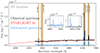 |
Fig. B.2. The 1D spectrum extracted from the MUSE observations at the location of SN 2016adj with prominent nebular emission features from the host labeled. The underlying stellar population was estimated using STARLIGHT (red line) and subtracted from the observed spectrum. The resulting gas-phase spectrum is shown in blue. A single Gaussian function was then fit to the nebular lines plotted within the insets. Flux ratios of these lines combined with the calibrations of Marino et al. (2013) and Dopita et al. (2016) indicate gas-phase 03N2 meallicities of (12 + log10(O/H)) = 8.55 ± 0.18 dex and 8.71±0.18 dex, respectively. |
Finally, the Hα equivalent width measurement at the location is 171±5 Å, which is higher than the value measured at the segmented region, and is positioned within the top 10% of the PISCO sample. The ΣSFR = (4.94±0.17) ×10−4 M⊙ yr−1 kpc−2, is also higher than the average of the PISCO sample, and completely consistent with the values inferred above.
On the other hand, the mere observation of a CC SN in Centaurus A is consistent with the idea presented by Della Valle & Panagia (2003) that repeated episodes of interaction and/or merging of early type galaxies with dwarf companions, on time scales of about 1 Gyr, are responsible both for inducing a strong radio activity observed in about 10% early type galaxies, and for supplying a consistent number of CC SN progenitors to the stellar population of elliptical galaxies. Della Valle et al. (2005) estimated that CC events should occur in these systems at a rate of up to 10% SNe-Ia. However, this is still not the probability of detecting CC-SNe in radio-galaxies because, on average, they are fainter at peak luminosity than SNe-Ia and therefore suffer from an obvious observational bias emphasized by the presence of a massive dust lane as observed, for example, in Centaurus A.
Appendix C: Pre-explosion progenitor analysis
Here we detail our efforts in analyzing pre-explosion images of Centaurus A.
C.1. AO imaging
The ESO archive was used to identify deep images of Centaurus A obtained prior to the discovery of SN 2016adj. Fortuitously, the galaxy was observed on 2008 June 30 with the VLT (+NACO) equipped with J, H and Ks filters. The data were taken with the S27 camera (FOV is 28×28 arcsec with 27 mas pixels), and reduced reduced using ESOREX scripts. In brief, the reduction process consisted of dark subtraction, flat fielding, and sky subtraction using off target sky frames. Given that in most frames the site of SN 2016adj fell outside the FOV, we were left with only a single 180 s exposure in H and Ks. In the case of J band, where there were 2x180 s images, we co-added these into a single deeper image. We measured the FWHM of the Ks-band image to be 2.8 pixels (0 08).
08).
We also retrieved from the ESO archive adaptive optics (AO) Ks-band imaging of SN 2016adj taken with the VLT+NACO on the night of 2016 February 28. The S54 camera was used, which samples a 56×56″ field of view (FOV) with 54 mas pixels. The AO correction was obtained using the SN itself as a natural guide star. As SN 2016adj was extremely bright at the time of these observations, short 60 s exposures (DIT=0.4 s, NDIT=150) off-source sky frames were interleaved with on-source observations in order to accurately remove the sky background. The raw data were reduced using ESOREX, to give a final deep stacked image with exposure time 1920 s.
Unfortunately, NACO exhibited additional noise at the time of these observations that resulted in a pattern of horizontal stripes superimposed on each image. As this pattern is different in each quadrant of the detector, we only concern ourselves with the quadrant containing the position of SN 2016adj. We used a custom script to model the pattern of stripes and remove them from the stacked image. The final image therefore has a smaller FOV than the full S54 camera, but contains only minimal residual signs of the pattern of stripes. The FWHM of several point sources in the Ks-band image reveal an impressive image quality measurement of  .
.
In order to locate the position of SN 2016adj on the pre-explosion images, we aligned the pre-explosion Ks-band image to the post-explosion Ks-band image. Fourteen point sources common to both frames were identified within a 5″ radius of SN 2016adj. Their positions were measured, and a geometric transformation was derived between the two images. The root-mean-square (rms) uncertainty on the transformation was 8 and 6 mas in the x and y direction, respectively (∼0.3 pixels on the pre-explosion frame). This lies close to, but offset from a nearby source located approximately 2 pixels to the N.
The proximity of the source to the N leads us to consider whether the uncertainty of the transformation might be underestimated. To test this further, a bootstrap calculation was performed. First, 10 of the 14 reference sources used for the image alignment were randomly selected, and then a geometric transformation was calculated for only this subset. We first tested a transformation that allowed for translation, rotation and separate scaling factors in both the x and y directions. We also tested a more flexible geometric transformation that included an additional polynomial term to account for any distortion between the two frames. In both cases, we drew a different random set of 10 sources 1000 times. The results of this test are presented in Fig. C.1. In all cases, we find the transformed position of SN 2016adj lies offset from the nearby source. The 1σ uncertainty in position from our bootstrap analysis is x = 0.12, y = 0.07 pixels, for the transformation with translation, rotation and scaling; and x = 0.15, y = 0.07 pixels, for the transformation with an additional polynomial term. We note that these uncertainties are smaller than those found originally when deriving the transformation.
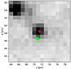 |
Fig. C.1. Pre-explosion NACO Ks-band image covering the position of SN 2016adj. The centroid of the nearby source is marked with a red cross, the transformed positions of the SN from our bootstrap analysis are plotted in green. |
From the preceding analysis, we conclude that the nearby source is likely not the progenitor of SN 2016adj. While the offset is very small (2 pixels, which is 0.9 pc at the distance of Centaurus A), this is more than 6σ from the transformed position of the SN. However, we note that there have been many cases of previous mis-identifications of SN progenitors (even using adaptive optics imaging, e.g., Maund et al. 2015). The proximity of SN 2016adj to the edge of the NACO FOV in the pre-explosion images is perhaps a cause for concern, as there may be some additional geometric distortion. However, this should be accounted for in the transformation with an additional polynomial term. In any case, the ultimate test is to obtain new, deep AO images of Centaurus A to test if the source to the N is still present after the SN has faded.
C.2. HST imaging
Centaurus A has been a frequent target of HST, and a number of pre-explosion images available in the HST archive cover the site of SN 2016adj. Some of these data were taken with older generation instruments (i.e., WFPC2) and have relatively low spatial resolution (0.1″pixels). However, Centaurus A was also observed with WFC3, and we list these pre-explosion observations in Table C.1.
HST pre-explosion observations covering the site of SN 2016adj.
To locate the position of SN 2016adj within the pre-explosion HST images, we used a set of HST (+WFC3) F814W images taken on 2016 February 22.04 UT. Four 40 s exposures were taken in order to avoid saturating on the bright SN, and we co-added these to produce a single image with total exposure time 160 s. This image was aligned to the pipeline-drizzled WFC3 F814W image taken on 2010 July 6.61 UT. This pre-explosion image has a pixel scale of 0 04.
04.
Twenty-five sources common to both images were identified, and using the matched list of pixel coordinates in the pre- and post-explosion frames, a geometric transformation was determined. The transformation allows for translation, rotation and a magnification factor in both x and y, as well as a polynomial term to account for any residual distortion. The rms uncertainty in the transformation is 0.11, 0.16 pixels in x and y, corresponding to 4 and 6 mas respectively.
We see a point source in the F814W image that lies slightly to the N of the transformed position of SN 2016adj, as shown in Fig. C.2. This nearby source is 1.6 pixels distant, or 64 mas, which is much greater than the uncertainty in our transformation, and consistent with the offset seen in the VLT+NACO data. We conclude that the nearby source is likely unrelated to SN 2016adj, and that the progenitor is not detected in these images.
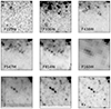 |
Fig. C.2. Cutouts ( |

C.3. Placing upper limits on the progenitor magnitude
While no progenitor candidate is identified in either HST or VLT pre-explosion images, we can still use these data to place limits on the magnitude of the progenitor. Using DOLPHOT, sources were injected into the images close to the transformed position of SN 2016adj. Fifty Monte Carlo trials were conducted for a range of injected source magnitudes, varying the pixel coordinates slightly each time. We define the limiting magnitude as the magnitude at which 50% of these sources are recovered within 0.2 mag of their injected magnitude. To determine this, a sigmoid function is fit to the recovered fraction as a function of magnitude. Resulting, robust limiting magnitudes are computed for the WFC3 F814W and F547M bands of > 26.4 and > 25.9 mag, respectively, while the bluer filters do not provide a robust constraint, nor does the F160W filter which is less sensitive than the VLT+NACO data.
We also used artificial star tests to determine a limiting magnitude for the NACO data. Here, we were presented with a number of challenges. The extremely small FOV of NACO meant that there were no bright, isolated sources within the FOV that could be used to determine a zeropoint (the nearby star at Ks = 9.2 mag is too bright). Moreover, the AO images have a spatially varying PSF across the FOV. So, we built a model of the PSF from nearby sources, and injected progressively fainter sources until they could no longer be comfortably recovered by eye. We determined the zeropoint for each image using standard stars observed on the previous or subsequent nights. The ESO weather archive suggests that all of these nights were photometric, and so we averaged each measurement of the zeropoint for each filter, rejecting points that lie > 3σ from the instrumental zeropoint as given by the NACO webpages. We were left with final limiting magnitudes of J > 21.6, H > 20.9 and Ks > 21.1 mag.
C.4. Luminosity limits on the progenitor of SN 2016adj
To summarize the preceding sections, we see a source close to, but significantly offset from the position of SN 2016adj in both HST and VLT+NACO pre-explosion images. Independent analyses using either the HST or NACO data each suggest that this is not the progenitor at greater than 6σ confidence.
We are hence left with a set of upper limits on the absolute magnitude of the progenitor of F547M > 25.9, F814W > 26.4, J > 21.6, H > 20.9, and Ks > 21.1 mag. Given our adopted distance and reddening of SN 2016adj (Sect. ??, 4.2), the absolute magnitude of the progenitor of SN 2016adj must be F547M > −8.4, F814W > −5.7, J > −8.2, H > −8.2, Ks > −7.5 mag.
Even for our deepest optical limit (F814W > −5.7 mag), only a handful of the brightest WR stars would be detected (Eldridge et al. 2013; Massey 2002). If the progenitor of SN 2016adj were a lower mass (and lower luminosity) star that had been stripped in a binary, then the optical limits are even less constraining.
While WR stars emit most of their luminosity at UV wavelengths, if they are surrounded by significant CSM it is possible that some of this UV radiation is reprocessed to the infrared. To establish whether the NIR limits are useful, we compare to the catalog of MW WR stars in Rate & Crowther (2020). The WC stars in this catalog have Ks absolute magnitudes ranging from ∼ − 3.5 (for early WC stars) to ∼ − 7 for late type WC stars. Only the brightest WC star in their sample had a Ks-band magnitude sufficient that we would see it in our NACO data. As for the optical, we hence conclude that we cannot use these data to place meaningful limits on the progenitor.
C.5. Searching for a progenitor in F555W through host-galaxy subtraction
While no obvious candidate is identified in the pre-explosion F555W images, the availability of late-time HST data after the SN has faded allowed us to make a final test. We took the 2000s F555W pre-explosion image from 1997 August 01.88 UT, and aligned it to the late time HST (+ WFC3) UVIS image taken on 2021 July 28.6 UT. After resampling the latter to match the pixel scale and orientation of the former, the HOTPANTS package was used to perform difference imaging between the two images. The results of this subtraction can be seen in Fig. C.3; while the light echo emission around SN 2016adj is clearly visible in the subtracted late phase image (see also Stritzinger et al. 2022), there is no sign of a change in flux at the position of SN 2016adj.
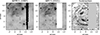 |
Fig. C.3. Subtraction between pre-explosion WFPC2+F555W filter image, an the late time WFC3+F555W image, covering the site of SN 2016adj. The WFC3 image has been transformed to match the pixel scale of the WFPC2 data. A diffraction spike from the nearby bright star in the field is visible in the WFPC2 image, and is masked in the WFC3 image. No disappearing progenitor can be seen in the subtracted image, although signatures of light echo emission are clearly visible. |
Appendix D: CO modeling details
Fig. D.1 displays the corner plot associated with our MCMC calculations that led us to determine the best CO model fit discussed in Sect. 7. The corner plot displays the PDF (posterior probability functions) computed for the six model-fit parameters.
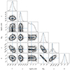 |
Fig. D.1. Posterior distribution of the MCMC parameters used to determine the best fit. |
All Tables
All Figures
|
Fig. 1. Colored image of Centaurus A (NGC 5128) constructed from RGB images obtained with the Swope telescope located at the Las Campanas Observatory. SN 2016adj occurred within the central dust lane, just southeast of a very bright, and typically saturated foreground star. |
| In the text | |
|
Fig. 2. Optical spectra of SN 2016adj from −7 days to +156 days. Phase and telescope facility are indicated on the right of each spectrum. Prevalent spectral features are marked with vertical dashed lines and labeled. Telluric absorption features are labeled with Earth symbols, while for the +43 days to +49 days spectra possible over-subtraction of host-galaxy Hα emission is masked by a translucent black region (see Appendix A.2 for details). |
| In the text | |
|
Fig. 3. Measurements of −vabs for a handful of mostly prominent features (see legend) in the optical and NIR spectra of SN 2016adj, plotted vs. days relative to the epoch of the B-band maximum. |
| In the text | |
|
Fig. 4. NIR spectral time series of SN 2016adj covering 6 months of evolution beginning from the epoch of the B-band maximum. The phase and telescope are indicated to the right of the spectra. The locations of various spectral features are identified with vertical dashed lines and labeled. The lines indicate the spectra where the features are identified. Telluric regions were labeled with an Earth symbol. |
| In the text | |
|
Fig. 5. Potential signatures of an interaction with circumstellar hydrogen. Top: Low-resolution optical- +116 days and middle: echelle NIR +97 days spectra of SN 2016adj. The optical and NIR spectra have been color-corrected to match coeval broad-band photometry. Both spectra are de-reddened using the reddening parameters estimated in Sect. 4.2. The positions of conspicuous hydrogen features are marked with vertical lines and labeled. Bottom: Zoom in velocity space of the Balmer, Paschen and Bracket series features. The Paschen features exhibit P Cygni profiles with −vabs values ∼1500 − 3000 km s−1 and vFWHM ∼ 1000 km s−1. The red lines correspond to pseudo-continuum fits determined by Monte Carlo simulations. We note that the flux of the nebular [N II] λλ6548,6584 lines on either side of Hα is not included in its emission-line flux measurement. |
| In the text | |
|
Fig. 6. Selection of optical spectra of SN 2016adj de-reddened and compared with similar phase spectra of the type IIb SN 2011dh (Ergon et al. 2014), the type Ib SN 2007Y (Stritzinger et al. 2009), and the type Ic SN 2005az (Bianco et al. 2014; Modjaz et al. 2014). The epochs labeled next to each spectra are relative to the epoch of r-band maximum. Similar to the type Ic SN 2005az, the spectra of SN 2016adj lack Balmer lines (dashed magenta) and He I features (red dash lines), both of which develop past maximum in the SNe 2007Y and 2011dh. C II lines are indicated with blue dashed lines. |
| In the text | |
|
Fig. 7. De-reddened NIR spectrum of SN 2016adj taken at +32 days compared with a +15 days spectrum of the type Ic SN 2007gr (Valenti et al. 2008), a +16 days spectrum of the type IIb SN 2011dh (Ergon et al. 2014), and the SYNOW synthetic spectrum computed for C I (Millard et al. 1999). Prevalent C I lines, as for example the strong feature around 11 000 Å, are present in the NIR spectrum of SN 2016adj. As in the optical, no traces of He I are identified in the longer wavelength spectrum of SN 2016adj. This is contrary to the He I features in the spectrum of SN 2011dh, particularly the prevalent P Cygni feature at 20 581 Å. |
| In the text | |
|
Fig. 8. Optical and NIR photometry of SN 2016adj plotted relative to the epoch of the B-band maximum from observations obtained by CSP-II, PESSTO, with the ESO-Paranal VLT Survey Telescope (VST) equipped with OmegaCAM, and with the UVOT camera on board Swift. To facilitate the comparison of photometry obtained with different instruments, in some cases offsets have been applied as indicated in the legend. A low-order polynomial function is overplotted on each light curve and used to infer the time and value of peak. Epochs of spectroscopic observations are indicated by black (visual) and red (NIR) segments. |
| In the text | |
|
Fig. 9. Optical and optical/NIR colors of SN 2016adj corrected for Milky Way reddening (filled symbols) vs. days relative to the time of the V-band maximum. The solid lines correspond to the SN Ic intrinsic color-curve templates presented by Stritzinger et al. (2018), while the unfilled symbols correspond to the fit of the templates to the filled symbols. The E(V − H)host color excess suggests an |
| In the text | |
|
Fig. 10. Optical and NIR E(V − X)host (where X = u, B, g, r, i, Y, J, H) color excess measurements of SN 2016adj, plotted as a function of the effective wavelength of passband X. Each color excess measurement represents the difference between the observed color (corrected for E(B − V)MW) and the intrinsic color-curve template for SN Ic shown in Fig. 9. The red dashed line corresponds to the best Fitzpatrick (1999) reddening law model fit characterized by a ratio of total-to-selective absorption |
| In the text | |
|
Fig. 11. Comparison of the −1.6 days spectrum of SN 2016adj de-reddened for Milky Way reddening and also assuming the two different sets of reddening parameters discussed in Sect. 4.2 and indicated in the plot. Also plotted in green is the CSP-I SN Ic spectral template at +0 days (Holmbo et al. 2023). |
| In the text | |
|
Fig. 12. Absolute magnitude light curves of SN 2016adj compared to the CSP-I SE SN template light curve scaled in time and to the average peak absolute magnitude determined from the CSP-I SN Ic sample. The light curves of SN 2016adj are plotted with and without host-extinction correction as indicated in the legend. The prevalent reddening is visible in the bluer bands with the Milky Way reddening corrected light curves of SN 2016adj being much fainter compared with the average SN Ic light curves. Also shown for comparison are the light curves of the type Ic SN 2005az (Bianco et al. 2014) which, as demonstrated in Fig. 6, is spectroscopically similar to SN 2016adj. The error bars accompanying the magnitudes of SN 2016adj account for the uncertainties in the distance and the reddening parameters |
| In the text | |
|
Fig. 13. Bolometric light curves (top), black-body temperature profile (middle), and black-body radius profile (bottom) of SN 2016adj. Using broadband photometry corrected for both Milky Way and host-galaxy reddening, bolometric light curves were computed by: (i) integrating the best-fit Planck function to the SEDs (dashed line denoted by LBB), (ii) trapezoidal integration of the SEDs (filled squares denoted by L∫) and (iii) through the combination of the g- and i-band photometry combined with the bolometric corrections presented by Lyman et al. (2014, filled circles denoted LBC, Lyman). We adopted our best host-reddening estimate, that is, a FTZ99 reddening law with |
| In the text | |
|
Fig. 14. Observed i-band photometry of SN 2016adj in flux units (black symbols) vs. days relative to the estimated explosion epoch (JD–2457411.5 ± 2.5). Overplotted as a blue solid line is the SN Ib/c i-band template light curve presented by Taddia et al. (2015), scaled and shifted to match the light curve of SN 2016adj. The blue dashed lines corresponds to a 1-σ uncertainty error snake. The epoch of the inferred explosion time, t0, is indicated by the vertical red solid line and assumes an i-band rise time of 21 days (see Taddia et al. 2015). The time difference between the inferred explosion date and the first i-band epoch is 2.5 days, which corresponds to the uncertainty of our estimated rise time. |
| In the text | |
|
Fig. 15. Pseudo-bolometric light curve of SN 2016adj constructed with the bolometric corrections from Lyman et al. (2014) and plotted along with our best-fit Arnett (1982) model. The model was fit to the luminosity measurements shown in blue and consisting of epochs extending up to 61 days post explosion when the ejecta remains to be optically thick to the gamma-rays emitted by radioactive decay (see Taddia et al. 2018b, and references therein). |
| In the text | |
|
Fig. 16. First CO overtone feature in the +97 days NIR medium-resolution spectrum of SN 2016adj (solid black line) compared with the best-fit model (solid red line) characterized by the parameters listed in the legend. The dot-dashed black line corresponds to the underlying continuum flux. |
| In the text | |
|
Fig. 17. Cartoon of SN 2016adj experiencing a circumstellar interaction (CSI). Left: H-rich shell located within Ds ∼ 0.007 pc of an infant SN delimited with a cavity formed by its progenitor WR wind. The expanding SN ejecta is indicated, along with the CO freshly synthesized within the wake of the SN ejecta. Right: schematic after the shell has been shocked by the expanding SN ejecta. CSI produces both forward and reverse shocks, and the ionization of hydrogen. |
| In the text | |
|
Fig. A.1. Sections of post maximum NIR spectra of SN 2016adj plotted in velocity space and centered on the rest wavelengths of five Paschen spectral lines. Vertical dashed lines coincide with the spectra exhibiting Paschen features in Pa-δ, Pa-γ, and Pa-β. For Pa-ζ, it indicates a potential detection, whereas Pa-α lacks evidence of a feature (see Table 3 for a summary of line identifications). |
| In the text | |
|
Fig. A.2. Steps of host-galaxy template subtraction. Top left: Optical-band science image created from stacking multiple images and zoomed in on the location of SN 2016adj. North is up and east is to the left. Top right: Residual obtained after subtraction of a modeled PSF from the PSF of the bright foreground star located in close proximity to SN 2016adj. Bottom right: Mask applied to the residual of the bright star. Bottom left: Region surrounding SN 2016adj copied into the initial science image after performing host-galaxy template subtraction of the masked science image. |
| In the text | |
|
Fig. A.3. Shown in the right panel is the NTT +EFOSC2 one-dimensional spectrum obtained on 2016 April 4.3 UT and extracted without background subtraction (red), and with background subtraction (black) using three slightly different background regions, as indicated in the left panels. Each of the extracted spectra reveals a feature which if associated with Hα would imply a −vabs = 1, 500 km s−1. |
| In the text | |
|
Fig. B.1. Spaxel binned MUSE data cube revealing (from left to right) the Hα flux (panel 1), the Balmer decrement-based |
| In the text | |
|
Fig. B.2. The 1D spectrum extracted from the MUSE observations at the location of SN 2016adj with prominent nebular emission features from the host labeled. The underlying stellar population was estimated using STARLIGHT (red line) and subtracted from the observed spectrum. The resulting gas-phase spectrum is shown in blue. A single Gaussian function was then fit to the nebular lines plotted within the insets. Flux ratios of these lines combined with the calibrations of Marino et al. (2013) and Dopita et al. (2016) indicate gas-phase 03N2 meallicities of (12 + log10(O/H)) = 8.55 ± 0.18 dex and 8.71±0.18 dex, respectively. |
| In the text | |
|
Fig. C.1. Pre-explosion NACO Ks-band image covering the position of SN 2016adj. The centroid of the nearby source is marked with a red cross, the transformed positions of the SN from our bootstrap analysis are plotted in green. |
| In the text | |
|
Fig. C.2. Cutouts ( |
| In the text | |
|
Fig. C.3. Subtraction between pre-explosion WFPC2+F555W filter image, an the late time WFC3+F555W image, covering the site of SN 2016adj. The WFC3 image has been transformed to match the pixel scale of the WFPC2 data. A diffraction spike from the nearby bright star in the field is visible in the WFPC2 image, and is masked in the WFC3 image. No disappearing progenitor can be seen in the subtracted image, although signatures of light echo emission are clearly visible. |
| In the text | |
|
Fig. D.1. Posterior distribution of the MCMC parameters used to determine the best fit. |
| In the text | |
Current usage metrics show cumulative count of Article Views (full-text article views including HTML views, PDF and ePub downloads, according to the available data) and Abstracts Views on Vision4Press platform.
Data correspond to usage on the plateform after 2015. The current usage metrics is available 48-96 hours after online publication and is updated daily on week days.
Initial download of the metrics may take a while.